Bayesian Analysis of Latent Variable Modelsusing Mplus

Tihomir Asparouhov and Bengt MuthenVersion 4

September 29, 2010

1

1 Introduction

In this paper we describe some of the modeling possibilities that are nowavailable in Mplus Version 6 with the Bayesian methodology. This newmethodology offers many new possibilities but also many challenges. Thepaper is intended to spur more research rather than to provide complete an-swers. Recently there have been many papers on Bayesian analysis of latentvariable models. In this paper we do not provide a review of the existingliterature but rather emphasize the issues that have been overlooked up tonow. We use the Bayesian methodology in the frequentist world and com-pare this methodology with the existing frequentist methods. Here we do notprovide details on the algorithms implemented in Mplus, but such details areavailable in Asparouhov and Muthen (2010). We focus instead on simulationstudies that illuminate the advantages and disadvantages of the Bayesianestimation when compared to the classical estimations methods such as themaximum-likelihood and weighted least squares estimation methods.

2 Factor Analysis

2.1 Factor Analysis with Continuous Indicators

In this section we evaluate the Bayes estimation of a one factor analysismodel with a relatively large number of indicators P = 30 and a small num-ber of indicators P = 5. As we will see having a large number of indicatorsis more challenging than one would expect in MCMC because it creates ahigh correlation between the generated factors and the loadings. We con-sider three different parameterizations. Denote by parameterization ”L” theparameterization where all loadings are estimated and the factor varianceis fixed to 1. The parameterization ”V” is the parameterization where thefirst factor loading is fixed to 1 and the variance of the factor is estimated.The parameterization PX is the extended parameter parameterization whereboth the variance and the first loadings are estimated. This model is formallyspeaking unidentified however the standardized loadings are still identified.These standardized loadings are obtained by

λs = λ√ψ

where λs is the standardized loading, λ is the unstandardized loading andψ is the factor variance. The loadings λs are essentially equivalent to the

2

loadings in parameterization ”L”. The ”PX” parameterization idea has beenused with the Gibbs sampler for example in van Dyk and Meng (2001) andGelman et al. (2008b).

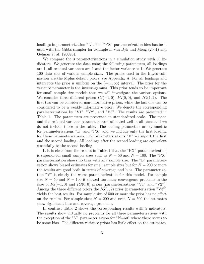
We compare the 3 parameterizations in a simulation study with 30 in-dicators. We generate the data using the following parameters, all loadingsare 1, all residual variances are 1 and the factor variance is 1. We generate100 data sets of various sample sizes. The priors used in the Bayes esti-mation are the Mplus default priors, see Appendix A. For all loadings andintercepts the prior is uniform on the (−∞,∞) interval. The prior for thevariance parameter is the inverse-gamma. This prior tends to be importantfor small sample size models thus we will investigate the various options.We consider three different priors IG(−1, 0), IG(0, 0), and IG(1, 2). Thefirst two can be considered non-informative priors, while the last one can beconsidered to be a weakly informative prior. We denote the correspondingparameterizations by ”V1”, ”V2”, and ”V3”. The results are presented inTable 1. The parameters are presented in standardized scale. The meanand the residual variance parameters are estimated well in all cases and wedo not include those in the table. The loading parameters are symmetricfor parameterizations ”L” and ”PX” and we include only the first loadingfor these parameterizations. For parameterizations ”V” we report the firstand the second loading. All loadings after the second loading are equivalentessentially to the second loading.

It it is clear from the results in Table 1 that the ”PX” parameterizationis superior for small sample sizes such as N = 50 and N = 100. The ”PX”parameterization shows no bias with any sample size. The ”L” parameteri-zation shows biased estimates for small sample sizes but for N = 200 or morethe results are good both in terms of coverage and bias. The parameteriza-tion ”V” is clearly the worst parameterization for this model. For samplesize N = 50 and N = 100 it showed too many convergence problems in thecase of IG(−1, 0) and IG(0, 0) priors (parameterizations ”V1” and ”V2”).Among the three different priors the IG(1, 2) prior (parameterization ”V3”)yields the best results. For sample size of 500 or more the prior has no effecton the results. For sample sizes N = 200 and even N = 500 the estimatesshow significant bias and coverage problems.

In contrast Table 2 shows the corresponding results with 5 indicators.The results show virtually no problems for all three parameterizations withthe exception of the ”V” parameterization for ”N=50” where there seems tobe some bias. The different variance priors has little effect on the estimates.

3

Table 1: Bias(coverage) for one factor model with 30 indicators.

Parameter- Para-ization meter N=50 N=100 N=200 N=500 N=1000 N=5000

L λ1 0.59(47) 0.17(76) 0.07(87) 0.02(91) 0.01(97) 0.00(90)PX λ1 0.03(92) 0.00(95) 0.00(96) -0.01(97) 0.00(98) 0.00(91)V1 λ1 - - -0.26(41) -0.07(76) -0.03(89) -0.01(89)V1 λ2 - - 0.00(98) 0.00(96) 0.00(96) 0.00(93)V2 λ1 - - -0.31(34) -0.08(73) -0.03(89) -0.01(88)V2 λ2 - - 0.00(98) 0.00(96) 0.00(96) 0.00(93)V3 λ1 -0.59(0) -0.41(17) -0.18(47) -0.07(78) -0.03(90) -0.01(89)V3 λ2 0.40(64) 0.05(95) 0.01(98) 0.00(97) 0.00(96) 0.00(93)

Thus we conclude that the problems we see in the Bayes estimation arespecific to the large number of indicators. The larger the number of indicatorsthe bigger the sample size has to be for some of the above parameterizationsto yield good estimates. While the 3 parameterizations use different priorssettings the difference in the results is not due to the priors but it is dueto the different mixing in the MCMC chain. If all chains are run infinitelylong the results would be the same or very close, however running the chaininfinitely long is only an abstract concept and therefore it is important toknow which parameterization is best for which model.

The above simulation shows that the more traditional parameterizations”V” and ”L” are fine to use unless the number of indicators is large and thesample size is small. In this special case one needs to use the more advancedparameterization ”PX”. As the number of indicators increases the minimalsample size for the ”L” parameterization and the ”V” parametrization willgrow. The simulations also show that the parameterization ”L” is somewhatbetter than parameterization ”V” when the sample size is small.

4

Table 2: Bias(coverage) for one factor model with 5 indicators.

Parameter- Para-ization meter N=50 N=100 N=200 N=500 N=1000 N=5000

L λ1 0.04(98) 0.04(95) 0.03(95) 0.02(94) 0.01(93) 0.00(94)PX λ1 0.00(94) 0.02(98) 0.02(95) 0.01(96) 0.01(94) 0.00(93)V1 λ1 -0.15(87) -0.03(97) 0.00(96) 0.00(98) 0.00(96) 0.00(95)V1 λ2 0.02(95) -0.01(96) 0.00(97) 0.00(92) 0.00(91) 0.00(96)V2 λ1 -0.07(100) -0.07(96) -0.02(97) 0.00(98) 0.00(96) 0.00(95)V2 λ2 0.04(97) 0.01(97) -0.01(97) 0.00(92) 0.00(92) 0.00(96)V3 λ1 -0.15(87) -0.03(97) 0.00(96) 0.00(98) 0.00(96) 0.00(95)V3 λ2 0.02(95) -0.01(96) 0.00(97) 0.00(92) 0.00(91) 0.00(96)

2.2 The Advantages of Improper Priors

In this section we present two examples that demonstrate the advantages ofthe improper priors used as defaults in Mplus for the variance parameters.Basic information regarding priors and the Mplus defaults is available inAppendix A. If there is one factor in the model Mplus uses by default theIG(−1, 0) prior for the factor variance and if there are more than one factorsit uses IW (0,−m − 1) where m is the number of factors. Both of thesepriors have a uniform density over its domain. In this section we use theV parameterization in the factor analysis models, i.e., one factor loading isfixed to 1 for each factor and the variance covariance matrix of the factorsis estimated. In the next two sections we present two examples. The firstexample is based on a one factor model. The second example is based on atwo factor model. Both examples use normally distributed variables.

2.2.1 One Factor Model

In this section we consider a factor model with one factor and 3 indicatorvariables. The model is given by the following equation

yj = µj + λjη + εj.

We generate 100 data sets of sample size N . To generate the data we set allparameters to 1, including the loading parameters, the intercept parameters

5

Table 3: Absolute bias (percent coverage) for ψ in one factor analysis model.

Prior N=50 N=100 N=200 N=500IG(0, 0) 0.16(91) 0.12(92) 0.04(93) 0.03(93)IG(−1, 0) 0.03(94) 0.00(93) 0.01(90) 0.01(93)

and the variance parameters for the factor and the residual variables. Wereport the results only for the factor variance parameter ψ as this parameterappears to be the most sensitive to the choice of the prior but the rest of theparameters are also affected in a similar way. We estimate the model usingtwo different priors for the factor variance both of which can be considerednon-informative: IG(−1, 0) and IG(0, 0). Table 3 contains the bias and thecoverage for the factor variance estimates. We can see that the IG(0, 0)prior yields some bias in the estimates particularly for the small sample sizesituations while the IG(−1, 0) prior yields nearly unbiased estimates. Thisbias advantage of the IG(−1, 0) prior also results in MSE advantage as well.

The simulation results also show that the effect of the prior on the esti-mates is negligible as the sample size increases to N = 500 and in that caseboth priors perform well.

2.2.2 Two Factor Model

In this section we consider a two factor analysis model where each factor has3 indicator variables. The model is given by the following two equations. Forj = 1, ..., 3

yj = µj + λjη1 + εj (1)

and for j = 4, ..., 6yj = µj + λjη2 + εj. (2)

We generate 100 data sets of sample size N . To generate the data we usethe following parameter values. The loading parameters λj are set to 1, theintercept parameters µj are set to 20, the variance parameter for ηj and εjare set to 20. The covariance parameter ρ between the two factor variablesη1 and η2 is set to 10. We estimate the model given in equations (1) and (2)using the V parameterization where the factor loadings λ1 and λ4 are fixedto 1 and the variance covariance matrix Ψ for the two factors is estimated.

6

Table 4: Absolute bias (percent coverage) for λ2 in two factor analysis model.

Prior N=50 N=100 N=200 N=500IW (I, 3) 2.09(64) 0.32(85) 0.08(88) 0.03(94)IW (0, 0) 2.82(91) 0.11(91) 0.04(94) 0.01(94)IW (0,−3) 0.02(95) 0.01(95) 0.00(96) 0.00(95)

We estimate the model using three different priors for Ψ all of which canbe considered non-informative or weakly informative. The first prior is theMplus default prior IW (0,−m−1), where m is the size of the Ψ matrix. Forthis model this is the prior IW (0,−3). The other two priors that we use areIW (0, 0) and IW (I, 3), where I is the identity matrix.

In Table 4 we report the results only for the loading parameter λ2. Theresults for the rest of the parameters are similar. We can see that the IW (0, 0)and IW (I, 3) priors yield bias estimates particularly for the small sample sizesituations while the IW (0,−3) prior yields unbiased estimates in all cases.

In these simulation results we see again that the effect of the prior on theestimates is negligible as the sample size increases to N = 500 and that allpriors perform well for large samples.

2.3 Centered Parameterization

Dunson et al. (2005) recommend the use of the so called centered parame-terization in structural equation models where not only the factor varianceis a free parameter as in the parameterization ”V” described in the previoussection but also the factor mean is a free parameter as well. In this param-eterization for identification purposes the intercept of one of the indicatorvariables is fixed to 0. We denote this parameterization by ”C”. The con-clusion in Dunson et al. (2005) is that the centered parameterization offersbetter mixing and faster convergence. The purpose of this section is to eval-uate the need for this parameterization in Mplus. The results in Dunsonet al. (2005) are obtained from an algorithm that differs from the Mplusalgorithm in one important aspect. In Mplus all latent variables are gener-ated as a block, i.e., they are generated simultaneously from a multivariatedistribution conditional on the observed data and the parameters. This pro-tects from a potentially poor mixing due to highly correlated draws for the

7

latent variables. In Dunson et al. (2005) as well as the WinBugs softwarethe latent variables are generated one at a time, i.e., from a univariate distri-bution conditional on the other latent variables, the observed data and theparameters.

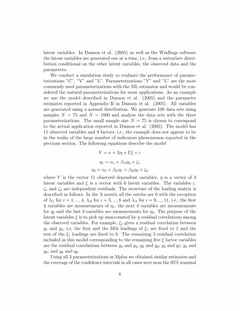
We conduct a simulation study to evaluate the performance of parame-terizations ”C”, ”V” and ”L”. Parameterizations ”V” and ”L” are the mostcommonly used parameterizations with the ML estimator and would be con-sidered the natural parameterizations for most applications. As an examplewe use the model described in Dunson et al. (2005) and the parameterestimates reported in Appendix B in Dunson et al. (2005). All variablesare generated using a normal distribution. We generate 100 data sets usingsamples N = 75 and N = 1000 and analyze the data sets with the threeparameterizations. The small sample size N = 75 is chosen to correspondto the actual application reported in Dunson et al. (2005). The model has11 observed variables and 9 factors, i.e., the example does not appear to bein the realm of the large number of indicators phenomenon reported in theprevious section. The following equations describe the model

Y = ν + Λη + Γξ + ε

η1 = α1 + β13η3 + ζ1

η2 = α2 + β21η1 + β23η3 + ζ2

where Y is the vector 11 observed dependent variables, η is a vector of 3latent variables and ξ is a vector with 6 latent variables. The variables ε,ζ1 and ζ2 are independent residuals. The structure of the loading matrix isdescribed as follows. In the Λ matrix all the entries are 0 with the exceptionof λi1 for i = 1, ..., 4, λi2 for i = 5, ..., 8 and λi3 for i = 9, ..., 11, i.e., the first4 variables are measurements of η1, the next 4 variables are measurementsfor η2 and the last 3 variables are measurements for η3. The purpose of thelatent variables ξ is to pick up unaccounted by η residual correlations amongthe observed variables. For example, ξ1 gives a residual correlation betweeny1 and y5, i.e, the first and the fifth loadings of ξ1 are fixed to 1 and therest of the ξ1 loadings are fixed to 0. The remaining 5 residual correlationincluded in this model corresponding to the remaining five ξ factor variablesare the residual correlations between y2 and y4; y2 and y6; y3 and y7; y4 andy8; and y6 and y8.

Using all 3 parameterizations in Mplus we obtained similar estimates andthe coverage of the confidence intervals in all cases were near the 95% nominal

8

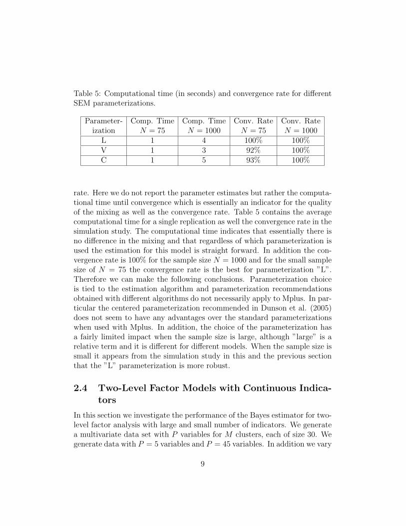
Table 5: Computational time (in seconds) and convergence rate for differentSEM parameterizations.

Parameter- Comp. Time Comp. Time Conv. Rate Conv. Rateization N = 75 N = 1000 N = 75 N = 1000

L 1 4 100% 100%V 1 3 92% 100%C 1 5 93% 100%

rate. Here we do not report the parameter estimates but rather the computa-tional time until convergence which is essentially an indicator for the qualityof the mixing as well as the convergence rate. Table 5 contains the averagecomputational time for a single replication as well the convergence rate in thesimulation study. The computational time indicates that essentially there isno difference in the mixing and that regardless of which parameterization isused the estimation for this model is straight forward. In addition the con-vergence rate is 100% for the sample size N = 1000 and for the small samplesize of N = 75 the convergence rate is the best for parameterization ”L”.Therefore we can make the following conclusions. Parameterization choiceis tied to the estimation algorithm and parameterization recommendationsobtained with different algorithms do not necessarily apply to Mplus. In par-ticular the centered parameterization recommended in Dunson et al. (2005)does not seem to have any advantages over the standard parameterizationswhen used with Mplus. In addition, the choice of the parameterization hasa fairly limited impact when the sample size is large, although ”large” is arelative term and it is different for different models. When the sample size issmall it appears from the simulation study in this and the previous sectionthat the ”L” parameterization is more robust.

2.4 Two-Level Factor Models with Continuous Indica-tors

In this section we investigate the performance of the Bayes estimator for two-level factor analysis with large and small number of indicators. We generatea multivariate data set with P variables for M clusters, each of size 30. Wegenerate data with P = 5 variables and P = 45 variables. In addition we vary

9

the size of the data set by varying the number of clusters M = 40, 80, 200or 500. We use a factor analysis model with one factor on the within leveland one factor on the between level. The model is given by the followingequation

Yjik = νj + λwjηwik + λbjηbk + εbjk + εwjik

where Yjik is the j−th observed variable, j = 1, ..., P , for observation i,i = 1, ...30 in cluster k, k = 1, ...,M . The latent factor variable ηwik is thewithin level factor variable for observation i in cluster k. The latent factorvariable ηbk is the between level factor variable for cluster k. The variablesεwjik and εbjk are the residual variables on the within and the between levelfor the j-th variable. To generate the data we use the following parametervalues. The loading parameters λwj and λbj are set to 1. The residualvariances and the factor variances are also set to 1. The intercept parameterνj is set to 0.

In this section we compare the PX and the L parameterizations. Inthis two-level estimation setup the total sample size is large, i.e., the withinlevel sample size is large. When the sample size is large the choice of theparameterization is irrelevant. Thus the choice of the parameterization onthe within level is irrelevant. For simplicity in all cases we choose the Lparameterization for the within level factor model. On the between levelhowever the sample size is small because it equals the number of clusters. Inmost practical applications and in this simulation the number of clusters isrelatively small. Therefore we can expect that the parameterization on thebetween level is important. In this section we compare only the PX and theL parameterization where this refers to the between level factor model.

We simulate 100 data sets with varying number of indicators and varyingnumber of clusters. Tables (6) and (7) contain the results of this simulation.For all parameters except the between level loading parameters the estimateand coverage are acceptable in all cases. Therefore in tables (6) and (7) weonly report the results for the first between level loading parameter. Theresults for the rest of the between level loading parameters are similar. Forthe case of M = 40, P = 45 with the L parameterization the convergencerate is only 35% and thus we do not report any results for this case. In allother cases the convergence rate is 100%. It is clear from these results thatas in the single level factor analysis model the L parameterization leads tobiased estimates with poor coverage when the number of indicators is largeand the number of clusters is small (M = 40, 80, 200). When the number

10

of indicators is small or the number of clusters is large (M = 500) the Lparameterization works well, the bias is small and the coverage is near thenominal level. On the other hand the PX parameterization works well in allcases in terms of both bias and coverage.

The implications of this simulation study are even more important forpractical purposes than those for single level factor analysis model. First inpractical applications the number of clusters is usually small. This occursmuch more frequently than small total sample size applications. Second, dueto the small number of clusters, it is common practice to have few betweenlevel factors. In situations when there are many factor indicator variables amodel is usually estimated with several factors on the within level but oneor two factors on the between level. This is common practice because a goodfit for the within-level variance covariance matrix usually requires severalfactors while a good fit for the between-level variance covariance matrix canbe achieved with only one or two factors. This is a simple consequence ofthe level specific sample size. The within level sample size (the total samplesize in the data) would be larger and misfits in the factor model are likelyto be significant. The between level sample size (the number of clusters)would be small and misfits in the factor model are likely to be insignificant.Thus more factors will be added on the within level and few on the betweenlevel to achieve a good fitting model. The consequence of this modeling ruleis that on the between level large number of indicators per factor would bequite common, i.e., the use of the PX parameterization for two-level modelsis critical.

To compute the PX parameterization we specify a unidentified modelwhere the factor variance and all factor loadings are free parameters. Con-sequently we compute the standardized estimates which are identified. Theunidentified estimates however can converge to infinity and cause numericalproblems in the estimation. To avoid this it may be necessary to add vaguebut proper priors for the loading parameters. In the above simulation weused a zero mean normal prior with variance 100. In addition, while com-puting the PX parameterization, Mplus Version 6 will monitor convergenceonly on the unidentified parameters. What is needed however is convergencefor the standardized parameters. To resolve this issue the MCMC chains arerun with a fixed number of iterations such as for example 10000 and thenthe standardized trace plots are inspected for convergence.

The above simulation shows that Bayes estimation of two-level factoranalysis is quite similar to the single level estimation with one exception.

11

Table 6: Absolute bias( percent coverage) for the first between level loadingin two-level factor model with 45 indicators.

Parameterization M=40 M=80 M=200 M=500L - 0.53(35) 0.12(74) 0.04(86)

PX 0.06(96) 0.00(93) 0.01(92) 0.00(94)

Table 7: Absolute bias(percent coverage) for the first between level loadingin two-level factor model with 5 indicators.

Parameterization M=40 M=80 M=200 M=500L 0.08(96) 0.03(95) 0.02(93) 0.00(90)

PX 0.01(94) 0.01(97) 0.01(91) 0.00(92)

While in single level estimation difficulties can arise when the sample size isclose to the number of variables, in two-level estimation we see these diffi-culties when the number of clusters is close to the number of variables.

2.5 Factor Analysis with Binary Indicators

In this section we consider some of the issues that arise in Bayesian factoranalysis with binary variables. Binary indicators provide more limited in-formation than continuous variables. If also the sample size is small andthe number of indicators is small there will be more limited information inthe data about the quantities that we are estimating. In this situation theestimates will depend on the priors. Consider a one factor model with five bi-nary indicators where all the thresholds are 0, all the loadings are 1, and thefactor variance is 1. We estimate this model with the parameterization ”L”.The default prior on each loading and threshold is the normal distributionwith zero mean and variance 5. We also consider three other priors: N(0, 1),N(0, 20) and N(0,∞). All of these priors are to some extent non-informativeand diffuse. Such priors are common in the IRT literature. For example, inFox and Glas (2001) the prior for the loadings are N(0,∞) constrained to allpositive values. In Segawa et al. (2008) the prior for the loadings is N(0, 105)constrained to (-25,5). In Patz and Junker (1999) the prior for the loading

12

is log-normal with mean 0 and variance 0.5. In Song et al. (2009) and Leeet al. (2010) similar but more complicated priors were used. In all of thesepapers however the sample size were large and the effect of the priors on theestimation is very small. Small sample size situations were not investigated.

In Gelman et al. (2008a) weakly informative priors, such as N(0, 1),N(0, 5) and N(0, 20), are recommended for logistic and probit regressionalthough preference is given there to priors based on the T-distribution andthe Cauchy distribution.

In this simulation we generate 100 data sets of different sample sizes andanalyze the data sets with each of these 4 prior assumptions for the loadings.The results are presented in Table 8. The table contains the bias and coverageonly for the first loading parameter. The remaining loading parameters aresimilar to the first loading. The threshold parameters are estimated well inall cases and we do not include these results. It is clear from these resultsthat the prior choice affects the results quite substantially for sample sizeN = 50 and N = 100 while for sample size N = 200 and bigger the effect ofthe prior is small or none at all. As the sample size increases the effect of theprior essentially disappears and the parameter estimates become the same asthe ML estimates. For small sample sizes the point parameter estimates areaffected dramatically by the prior. The best results are obtained with theN(0, 1) prior. Using N(0,∞) for parameters on the logit scale may actuallybe a very poor choice. Consider the implications of such a prior on R2 ofthe regression equation for each of the Y . The probability that R2 < 99% issmaller than R2 > 99%. It is obvious that this prior will be inappropriate formost situations and given that the priors have an effect on the results whenthe sample size is known a more thoughtful choice is needed. If no informativeprior is available, a prior related to the ML or WLSMV estimates for the samemodel may be a viable choice.

In Lee (2010) a similar conclusion has been reached. The authors statethat large sample sizes are required to achieve accurate results. Let’s againiterate and clarify this point. Bayesian estimation of structural models withcategorical variables show prior assumption dependence when the samplesize is small, for example N = 100. The results of the Bayesian estimationare accurate, however they depend on the prior assumptions. In these modelsall priors are informative since they affect the final result substantially. Thussetting up meaningful priors is very important. Setting up priors in thesemodels is also challenging because of the fact that the parameter are onprobit scale. It would be much easier to setup priors on probability scales

13

but that is not always possible.The prior assumption dependence may be a substantial hurdle in

practice, simply because good and meaningful priors are not easy to specify.This is particularly problematic when the Bayesian estimation is simply usedto obtain good point estimates and standard errors, because it is not clearhow to select priors that provide estimates with small or no bias. Our exam-ple shows however that simply avoiding the so called generic non-informativepriors is a good first step. For all parameters that are on probit scale itseems that specifying priors that have unlimited uniform range is not a goodidea because such priors induce skewed priors on probability scale. Instead,selecting priors with a reasonable and finite range is likely to yield betterresults.

The prior assumption dependence occurs for small sample sizes. Ev-ery model however will have a model specific sample size range where thisdependence occurs and we can not provide a general sample size range. How-ever the prior assumption dependence is easy to check. Simply estimat-ing the model with various different priors will show the degree to which theestimates depend on the priors.

Finally we are going to provide a frequentist interpretation on the pos-teriors and explain why priors can affect the results. Suppose that we drawparameters from the priors and then from those parameters and the model wedraw data sets similar to the observed data. We then remove all such drawsthat produce data different from the observed data and we retain all drawsthat produced data sets that are the same as the observed. The retainedparameters form the posterior distribution. Thus if two parameter values θ1and θ2 have been equally likely to produce the data the frequency ratio inthe posterior will be the same as that in the prior, i.e., the prior will have atremendous effect on the posterior when the data can not discriminate verywell between the parameters.

Note also that if the number of indicators is large in this factor analysismodel just as in the case of factor analysis model with continuous indicatorsthe PX parameterization has to be used otherwise the loading parameterswill be overestimated.

14

Table 8: Bias (percent coverage) for λ1,1 = 1 in factor analysis with binaryindicators.

Prior N=50 N=100 N=200 N=500N(0,∞) 3.41(84) 0.56(89) 0.11(92) 0.04(91)N(0, 20) 0.46(90) 0.34(88) 0.13(92) 0.04(92)N(0, 5) 0.30(93) 0.19(89) 0.09(92) 0.03(92)N(0, 1) 0.03(96) 0.07(93) 0.04(94) 0.01(93)

2.6 Factor Analysis with Multiple Factors

In this section we consider confirmatory factor analysis with multiple factorsand continuous indicators. We investigate the performance of the ”V” andthe ”L” parameterizations particularly for small sample size. Simulationstudy is conducted based on a factor analysis model with M factors whereeach factor is measured by 4 indicators. The model is described by thefollowing equation

Yj = µj + λjηm + εj

for m = 1, ...,M and j = 4m − 3, ..., 4m. We generate data according tothe above model using the following parameter values: µj = 0, λj = 1, theresidual variance θj = 1, and the factor variance covariance matrix Ψ hasall diagonal elements equal to 1 and all off diagonal elements equal to ρ.We generate 100 data sets of sample size N using the above model and weestimate the true model for each data set using both the ”V” and the ”L” pa-rameterizations. In the ”V” parameterization the first loading for each factoris fixed to 1, the remaining 3 loadings are estimated as free parameters andthe factor variance covariance matrix is estimated as a variance covariancematrix. In the ”L” parameterization for each factor all four loadings areestimated as free parameters but the variance covariance matrix is estimatedas a factor correlation matrix, i.e., the diagonal elements of Ψ are fixed to 1and all off diagonal elements are estimated. Both of these parameterizationsare frequently utilized for confirmatory factor analysis models with multiplefactors. In the simulation we vary the sample size N , the number of factorsM and the factor correlation ρ. We use sample sizes N = 100, 150 and 200,i.e., we focus on small sample size situations. The number of factors M is 3,4, or 5. The factor correlation ρ is 0.5, 0.6 or 0.75.

15

The results of this simulation study show that in all cases the param-eter estimates are unbiased and the coverage is near the nominal level forall parameters. Here we do not report these results. The main differencebetween the ”L” and the ”V” parameterizations that we found in this sim-ulation study is in the convergence rates. The convergence rate for the ”V”parameterization is always 100% while the convergence rate for the ”L” pa-rameterization slightly lower in some extreme cases. In Table 9 we report theconvergence rate for the ”L” parameterization under the various conditions.The convergence rate drops when the sample size is small and the number offactors is large and when the factor correlation is large.

16

Table 9: Convergence rate for the ”L” parameterization for CFA with mul-tiple factors. The convergence rate for the ”V” parameterization is 100% inall cases.

M ρ N Convergence Rate3 0.5 100 100%3 0.5 150 100%3 0.5 200 100%3 0.6 100 100%3 0.6 150 100%3 0.6 200 100%3 0.75 100 100%3 0.75 150 100%3 0.75 200 100%4 0.5 100 100%4 0.5 150 100%4 0.5 200 100%4 0.6 100 100%4 0.6 150 100%4 0.6 200 100%4 0.75 100 100%4 0.75 150 100%4 0.75 200 100%5 0.5 100 100%5 0.5 150 100%5 0.5 200 100%5 0.6 100 99%5 0.6 150 100%5 0.6 200 100%5 0.75 100 87%5 0.75 150 98%5 0.75 200 99%

17

3 Estimating Structural Equation Models With

Categorical Variables and Missing Data

The most popular method for estimating structural equation models with cat-egorical variables is the weighted least squares method (estimator=WLSMVin Mplus). This method however has certain limitations when dealing withmissing data. The method is based on sequentially estimating the univari-ate likelihood and then conditional on the univariate estimates the bivariatemodel is estimated. The problem with this approach is that when the miss-ing data is MAR and one dependent variable Y1 affects the missing datamechanism for another variable Y2, the two variables have to be estimatedsimultaneously in all stages of the estimation otherwise the estimates will bebiased.

Consider the following simple example. Let Y1 and Y2 be binary variablestaking values 0 and 1 and let Y ∗

1 and Y ∗2 be the underlying normal variables.

The relationship between Yi and Y ∗i is given by

Yi = 0⇔ Y ∗i < τi

for i = 1, 2 and parameters τi. Let τ1 = τ2 = 0. In that case P (Y1 = 0) =P (Y2 = 0) = 50%. Suppose also that the tetrachoric correlation between thetwo variables is ρ = 0.5. Suppose that the variable Y2 has missing values andthat the missing data mechanism is

P (Y2 is missing|Y1 = 0) = Exp(−2)/(1 + Exp(−2)) ≈ 12% (3)

P (Y2 is missing|Y1 = 1) = Exp(1)/(1 + Exp(1)) ≈ 73%. (4)

This missing data mechanism is MAR (missing at random). We simulate100 data sets according to this bivariate probit model of size 1000 and gen-erate the missing data according to (3) and (4). We then estimate the unre-stricted bivariate probit model with both the WLSMV and Bayes estimatorsin Mplus.

The results of the simulation study are given in Table 10. It is clearfrom these results that the WLSMV estimates are biased while the Bayesestimates are unbiased. The bias in the WLSMV estimates results in poorcoverage for that estimator, while the coverage for the Bayes estimator isnear the nominal 95% level.

18

Table 10: Comparing the WLSMV and Bayes estimators on bivariate MARdichotomous data.

True WLSMV Bayes WLSMV BayesParameter Value Estimates Estimates Coverage Coverage

ρ 0.50 0.35 0.51 0.14 0.88τ1 0.00 0.01 0.01 0.96 0.94τ2 0.00 0.23 -0.01 0.00 0.95

The same problem occurs for two-level models. Suppose that we have500 clusters of size 10 and two observed binary variables. The correspondingbasic bivariate two-level probit model for the two binary variables is givenby

Yi = 0⇔ Y ∗i < τi

Y ∗i = Yiw + Yib

for i=1,2. Here Yiw is a standard normal variable, i.e., Yiw has mean zero andvariance 1. The variable Yib has zero mean and variance vi. Both Yiw andYib are unobserved. There are two types of tetrachoric parameters in thismodel. On the within level we have the within level tetrachoric correlationρw between Y1w and Y2w. On the between level we have the between leveltetrachoric covariance ρb between Y1b and Y2b. We generate 100 data setsand we generate missing data using the missing data mechanism (3) and (4).We then analyze the data with the Bayes and WLSMV estimators in Mplus.The results of the simulation study are given in Table 11. We see that fortwo-level models the WLSMV estimates are again biased while the Bayesestimates are unbiased. The tetrachoric WLSMV estimates on both levelsare biased as well as the threshold WLSMV estimates.

The weighted least squares estimator relies on unbiased estimates of tetra-choric, polychoric and polyserial correlations to build estimates for any struc-tural model. If these correlation estimates are biased the structural parame-ters estimates will also be biased. Consider for example the growth model of5 binary variables observed at times t = 0, 1, 2, 3, 4. The model is describedby the following equation

P (Yit = 1) = Φ(η1i + tη2i).

19

Table 11: Comparing the WLSMV and Bayes estimators on bivariate two-level MAR dichotomous data.

True WLSMV Bayes WLSMV BayesParameter Value Estimates Estimates Coverage Coverage

ρw 0.50 0.40 0.51 0.08 0.91ρb 0.20 0.17 0.19 0.70 0.94v1 0.30 0.30 0.30 0.94 0.96v2 0.30 0.28 0.31 0.93 0.94τ1 0.00 0.00 0.00 0.95 0.93τ2 0.00 0.24 0.00 0.00 0.96

where Φ is the standard normal distribution function. The model has 5parameters: the mean µ1 of the random intercept η1i and the mean µ2 of therandom slope η2i as well as the variance covariance Ψ of these two randomeffects which has 3 more parameters. We generate 100 data sets of size1000 and we generate missing data for y2, y3, y4 and y5 via the missingdata mechanism described in (3) and (4), i.e., y1 affects the missing datamechanism for y2, ..., y4.

The results of this simulation study can be found in Table 12. We analyzethe data using the true model with several different estimators. We analyzethe data again with the WLSMV estimator directly and with the Bayes es-timators directly. The Bayes estimator we use two different priors for the Ψ,the uniform improper prior for all positive definite matrices IW (0,−3) andthe default proper prior IW (I, 3) which implies a more reasonable range forthe variance parameters as well as a uniform prior on (−1, 1) for the corre-lation parameter, see Appendix A. In addition to these estimators we alsoanalyze the data with the following estimators. Using the Mplus imputationmethod we analyze the data with the WLSMV estimator with 5 imputeddata sets as well as 50 imputed data sets. The multiple imputation methodis based on a Bayesian estimation of an unrestricted model which is then usedto impute the missing values. Multiple and independent imputations are cre-ated which are then analyzed using Rubin (1987) method. The unrestrictedmodel used for imputation is the the sequential regression with observed me-diators model which is the default method in Mplus for this kind of data.This approach was pioneered by Raghunathan et al. (2001). In addition, this

20

model can be analyzed with the ML estimator. The ML estimator is guar-anteed to provide consistent estimates since the missing data is MAR. Noteagain however that the ML estimator has some shortcomings that can not beovercome in general but for this particular model do not apply. The short-comings of the ML estimators is that it can only be used with no more than3 or 4 latent variables, otherwise the computational burden is so large thatit becomes impractical. Another shortcoming of the ML estimator is that itcan not be used with residual correlations between the categorical variablesbecause that would lead to the use of the multivariate probit function thatrequires computationally demanding numerical integration. Finally the MLestimator does not provide a model fit based on an unrestricted multivariateprobit model. The WLSMV estimator and the Bayes estimator both avoidthe above mentioned shortcomings. The parameter values used in this simu-lation study are as follows µ1 = 0.00, µ2 = 0.20, ψ11 = 0.50, ψ22 = 0.50, andψ12 = 0.30.

As expected again we see that the WLSMV estimates are biased whilethe Bayes estimates are close to the true values. In particular the mean ofthe random slope is underestimated dramatically by the WLSMV estimatorwhile the Bayes estimator is consistent. Also the coverage for the WLSMVestimator is unacceptable. In addition we see that the results between theBayes estimators with the two different priors are different and thus we haveprior assumption dependence for this model. Even though we have a samplesize of 1000, the growth model is somewhat difficult to identify because ituses only 5 binary variables. In this example again we see a clear advan-tage of using proper prior with bounded range rather than uniform improperprior. The proper prior leads to a decrease in the bias and improved cover-age. Overall the four estimators, the Bayes estimator with IW (I, 3) prior,the ML estimator, the WLSMV estimator with 5 imputed data sets, andthe WLSMV estimator with 50 imputed data sets performed very well andthere doesn’t appear to be a substantial difference between these estimators.Increasing the number of imputed data sets from 5 to 50 does not seem toimprove the results, i.e., 5 imputed data sets are sufficient. All of these 4 es-timators are computationally fast and while they are more involved than thetraditional WLSMV estimator, the improvement in the results is substantial.We conclude that in the presence of missing data the Bayes estimator offers avaluable alternative to the WLSMV estimator, both as a direct estimator oras an imputation method followed by the WLSMV estimator. The imputa-tion method followed by the WLSMV estimator however has the advantage

21

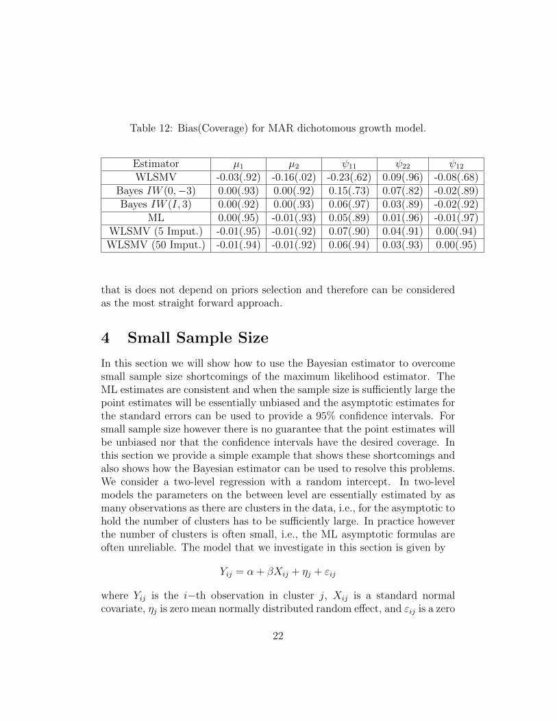
Table 12: Bias(Coverage) for MAR dichotomous growth model.

Estimator µ1 µ2 ψ11 ψ22 ψ12

WLSMV -0.03(.92) -0.16(.02) -0.23(.62) 0.09(.96) -0.08(.68)Bayes IW (0,−3) 0.00(.93) 0.00(.92) 0.15(.73) 0.07(.82) -0.02(.89)Bayes IW (I, 3) 0.00(.92) 0.00(.93) 0.06(.97) 0.03(.89) -0.02(.92)

ML 0.00(.95) -0.01(.93) 0.05(.89) 0.01(.96) -0.01(.97)WLSMV (5 Imput.) -0.01(.95) -0.01(.92) 0.07(.90) 0.04(.91) 0.00(.94)WLSMV (50 Imput.) -0.01(.94) -0.01(.92) 0.06(.94) 0.03(.93) 0.00(.95)

that is does not depend on priors selection and therefore can be consideredas the most straight forward approach.

4 Small Sample Size

In this section we will show how to use the Bayesian estimator to overcomesmall sample size shortcomings of the maximum likelihood estimator. TheML estimates are consistent and when the sample size is sufficiently large thepoint estimates will be essentially unbiased and the asymptotic estimates forthe standard errors can be used to provide a 95% confidence intervals. Forsmall sample size however there is no guarantee that the point estimates willbe unbiased nor that the confidence intervals have the desired coverage. Inthis section we provide a simple example that shows these shortcomings andalso shows how the Bayesian estimator can be used to resolve this problems.We consider a two-level regression with a random intercept. In two-levelmodels the parameters on the between level are essentially estimated by asmany observations as there are clusters in the data, i.e., for the asymptotic tohold the number of clusters has to be sufficiently large. In practice howeverthe number of clusters is often small, i.e., the ML asymptotic formulas areoften unreliable. The model that we investigate in this section is given by

Yij = α + βXij + ηj + εij

where Yij is the i−th observation in cluster j, Xij is a standard normalcovariate, ηj is zero mean normally distributed random effect, and εij is a zero

22

mean normal residual. The model has 4 parameters α, β, ψ = V ar(ηj), andθ = V ar(εij). We generate data according to this model using the followingparameter values α = 0, β = 1, ψ = 1, and θ = 2. We generate 100 data setswith M clusters each with 50 observations, i.e., the total sample size in eachdata set is 50M . We analyze the generated data with the ML estimator aswell as 3 different Bayes estimators. The Bayes estimators differ in the choiceof prior distribution for the parameter ψ. The Mplus default prior is theimproper prior IG(−1, 0) which is equivalent to a uniform prior on [0,∞).We also estimate the model with the priors IG(0, 0) and IG(0.001, 0.001)which have been considered in two-level models, see Browne and Draper(2006) and Gelman (2006).

The results for the parameter ψ are presented in Table 13. The bestresults in terms of bias and coverage are obtained with the Bayes estimatorand priors IG(0, 0) and IG(0.001, 0.001). The difference between the twopriors are essentially non-existent. The ML estimator shows low coverageeven for M = 20 and bigger bias even for M = 60. The Bayes estimatorwith default prior also performs poorly in terms of bias. Similar advantage ofthe Bayes estimator also occurs for the α parameter. This simulation showsthat when the number of clusters is smaller than 50 the Bayes estimator canbe used to obtain better estimates and more accurate confidence intervals intwo-level models particularly when the between level variance componentsuse priors such as IG(0, 0).

In Mplus the default for the variance on the between level random effectsis set to IG(−1, 0). Even though this prior yields less accurate results thanIG(0, 0), it is preferred in general as it has a greater chance for convergence.The prior IG(0, 0) has the tendency to pull small variance components, whichare common in two-level modeling, towards zero. This eventually leads tosingularity problems in the MCMC generation.

23

Table 13: Bias(Coverage) for ψ in two-level regression.

Estimator M=5 M=10 M=20 M=40 M=60ML -.22(.64) -.13(.82) -.09(.86) -.04(.91) -.03(.93)

Bayes IG(0.001,0.001) .13(.96) .01(.94) .03(.91) .01(.93) .01(.95)Bayes IG(0,0) .13(.96) .01(.94) .03(.93) .01(.93) .01(.95)Bayes IG(-1,0) 1.88( .89) .35(.95) .16(.88) .07(.91) .04(.93)

5 Bayesian Estimation as the Computation-

ally Most Efficient Method

In this section we describe models that are computationally challenging fortraditional estimation methods such as maximum-likelihood but are nowdoable with the Bayesian estimation.

5.1 Multilevel Random Slopes Models With Categor-ical Variables

Random effect models with categorical variables are usually estimated withthe ML estimator however each random effect accounts for one dimension ofnumerical integration. The ML estimator is not feasible when the dimensionof numerical integration is more than 3. Thus the maximum number of ran-dom effect the ML estimator can estimate in a two-level probit regression is3 (one intercept and 2 random slopes). It is possible to use Montecarlo inte-gration method with more than 3 random effects, however, such an approachusually require careful monitoring of the estimation. In particular the con-vergence in a maximum-likelihood estimation with Montecarlo integration issomewhat tricky because the usual methods that are based on monitoringthe log-likelihood value or the log-likelihood derivatives will be difficult touse due to larger numerical integration error.

In this section we will evaluate the performance of the Bayes estimatorfor q random effects for q = 1, ...6. The estimation time for the ML esti-mator grows exponentially as a function of the number of random effects.This however is not the case for the Bayesian estimation where the compu-

24

tational time grows linearly as a function of the number of random effects,i.e., increasing the number of random effects is not an obstacle for the Bayesestimation.

We conduct simulations with different number of random effects startingfrom 1 effect to 6 random effects. Let the number of random effects be q.To generate data for our simulation studies we first generate q covariates Xk

for k = 1, ..., q. We set X1 = 1 so that we include the random interceptin this model. For k = 2, ..., q we generate Xk as independent normallydistributed covariate with mean zero and variance 1. We also generate anormally distributed between level covariate W with mean 0 and variance 1.Let the binary dependent variable be U and denote by Uij the observation iin cluster j. The two-level binary probit regression is given by

P (Uij = 1) = Φ( q∑k=1

skjXkij

)skj = αk + βkWj + εkj

where εkj is a zero mean residual with variance covariance matrix Ψ of sizeq, i.e., the random effects are assumed to be correlated. We generate datausing these parameter αk = 0, Ψ = diag(0.5), βk = 0.7.

Using the Bayes estimator we analyze the generated data using each ofthese 3 different priors for Ψ: IW (0,−q−1), IW (I, q+1), and IW (2I, q+1),where I is the identity matrix, see Appendix A. The prior IW (0,−q−1) hasa constant density function over the definition domain, i.e., it is an improperuniform prior. The default IW (I, q+ 1) prior is usually selected as a properprior that has non-informative marginal distributions for the correlation pa-rameters, i.e., the marginal prior distribution for the correlations betweenthe random effects is uniform on [−1, 1]. The marginal distribution for thediagonal elements is IG(1, 0.5) which has mode at 0.25. The only differencebetween the prior IW (2I, q + 1) and IW (I, q + 1) is that the marginal priordistribution for the diagonal element of Ψ is IG(1, 1) which has a mode of 0.5.If we have a good reason to believe that the variances of the random effectsare near 0.5 (which is the true value here) then we can choose IW (2I, q+ 1)instead of IW (I, q+1) as a proper prior. In these simulations studies we gen-erate 200 clusters with 20 observations each for a total sample size of 4000.Note however that for the purpose of estimating the between level randomeffects distribution the sample size is 200, i.e., this sample size is within arange where the the prior assumptions can potentially affect the posterior.

25

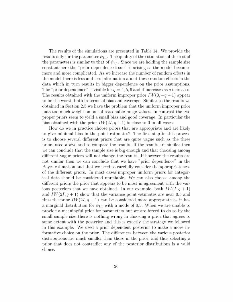
The results of the simulations are presented in Table 14. We provide theresults only for the parameter ψ1,1. The quality of the estimation of the rest ofthe parameters is similar to that of ψ1,1. Since we are holding the sample sizeconstant here the ”prior dependence issue” is arising as the model becomesmore and more complicated. As we increase the number of random effects inthe model there is less and less information about these random effects in thedata which in turn results in bigger dependence on the prior assumptions.The ”prior dependence” is visible for q = 4, 5, 6 and it increases as q increases.The results obtained with the uniform improper prior IW (0,−q− 1) appearto be the worst, both in terms of bias and coverage. Similar to the results weobtained in Section 2.5 we have the problem that the uniform improper priorputs too much weight on out of reasonable range values. In contrast the twoproper priors seem to yield a small bias and good coverage. In particular thebias obtained with the prior IW (2I, q + 1) is close to 0 in all cases.

How do we in practice choose priors that are appropriate and are likelyto give minimal bias in the point estimates? The first step in this processis to choose several different priors that are quite vague such as the threepriors used above and to compare the results. If the results are similar thenwe can conclude that the sample size is big enough and that choosing amongdifferent vague priors will not change the results. If however the results arenot similar then we can conclude that we have ”prior dependence” in theBayes estimation and that we need to carefully consider the appropriatenessof the different priors. In most cases improper uniform priors for categor-ical data should be considered unreliable. We can also choose among thedifferent priors the prior that appears to be most in agreement with the var-ious posteriors that we have obtained. In our example, both IW (I, q + 1)and IW (2I, q + 1) show that the variance point estimates are near 0.5 andthus the prior IW (2I, q + 1) can be considered more appropriate as it hasa marginal distribution for ψ1,1 with a mode of 0.5. When we are unable toprovide a meaningful prior for parameters but we are forced to do so by thesmall sample size there is nothing wrong in choosing a prior that agrees tosome extent with the posterior and this is exactly the strategy we followedin this example. We used a prior dependent posterior to make a more in-formative choice on the prior. The differences between the various posteriordistributions are much smaller than those in the prior, and thus selecting aprior that does not contradict any of the posterior distributions is a validchoice.

26

Table 14: Bias (percent coverage) for ψ1,1 = 0.5 in two-level probit regressionwith q random effects.

Prior q = 1 q = 2 q = 3 q = 4 q = 5 q = 6IW (0,−q − 1) 0.03(90) 0.04(92) 0.04(96) 0.08(81) 0.10(79) 0.19(60)IW (I, q + 1) 0.03(89) 0.02(93) -0.01(97) -0.01(95) -0.04(97) -0.05(92)IW (2I, q + 1) 0.03(89) 0.03(93) 0.01(97) 0.02(97) -0.01(97) -0.01(96)

5.2 Small Random Effect Variance

When the variance of a random effect is very small the EM algorithm hasa very slow rate of convergence even when aided by acceleration methods.On the other hand the Bayes estimator can take advantage of a prior spec-ification that avoids the variances collapsing to zero problem. The inversegamma prior will generally work well for this purpose, see Appendix A. Thenear zero variance for the random effect is a common problem in two-levelregression models. Once it is known that the variance is near 0 the correctmodeling approach is to replace the random effect coefficient with a standardregression coefficient. With such a specification the model will be much easierto estimate, however, typically we do not know that the variance is near zeroand thus estimate the effect as a random effect and frequently the ML estima-tion method will produce either very slow convergence or non-convergence.To illustrate this we conduct the following simulation study. Consider againthe two-level binary regression model as in the previous section

P (Uij = 1) = Φ( q∑k=1

skjXkij

)skj = αk + βkWj + εkj

where q = 3 and again the first covariate is set to the constant 1 to includethe random intercept in the model. Here we have one random interceptand two random slopes, i.e., the ML estimation will use only 3 dimensionalintegration which usually is not computationally heavy. We generate thedata using the following parameters α1 = 0, α2 = 0.2 and α3 = 0.2, βk = 0.7for k = 1, 2, 3. The two covariates on the within level X2 and X3 and the

27

between level covariate W are generated as standard normal variables. Theεk variables are generated as independent with variance ψ11 = ψ22 = 0.5 andψ33 = 0. The last parameter is the key parameter, i.e., the second randomslope has a zero variance. We generate 100 data sets each with 200 clusters ofsize 20 and analyze them with both the ML and the Bayes estimator. For theBayes estimation we use the Inverse-Wishart prior IW (I, 4) for the randomeffects variance covariance parameters, see Appendix A. For the αk and βkparameters we use uniform prior on (−∞,∞) interval, i.e., a non-informativeimproper prior.

The ML estimator took on average 19 minutes to complete each replica-tion while the Bayes estimator used only 5 seconds, i.e., the Bayes estimatoris about 200 times faster than the ML estimator. The results are presented inTable 15. The bias for both methods is near 0 and the coverage near the 95%nominal rate with one exception. The Bayes estimator does not ever includethe 0 value in the confidence interval for the variance parameter ψ33, i.e., thecoverage here is 0. This is always going to be the case. The posterior dis-tribution for a variance parameter consists only of positive values and sincethe inverse-gamma prior (which is the marginal distribution obtained fromthe inverse-wishart prior, see Appendix A) has low prior for near zero valuesthan even small positive values are not included in the posterior. Thus we seethat the Bayes estimator will necessarily estimate zero variances to small butpositive values, which essentially leads to the bias of 0.06 seen in Table 15.The Bayes estimator can not be used to test significance of the random effectvariance. The same is true for the standard LRT test because of borderlineissues that distort the LRT distribution. Instead DIC and BIC can be usedto evaluate the need for a random effect. Finally we conclude that the Bayesestimator avoids the collapse at zero of the variance parameter which in turnresults in mush faster estimation. However when the Bayes estimator gives asmall positive value for a variance parameter we should always suspect thatthe true value is actually zero.

28

Table 15: Bias (percent coverage) for small random effect variance estima-tion.

Parameter ML Bayesα1 0.01(90) 0.00(91)α2 0.01(95) 0.00(91)α3 0.00(96) 0.01(97)β1 0.01(96) 0.00(94)β2 0.00(98) 0.01(93)β3 0.00(95) 0.03(91)ψ11 0.01(96) 0.03(94)ψ22 0.01(93) 0.03(94)ψ33 0.01(99) 0.06(0)ψ12 0.00(97) 0.00(94)ψ13 0.00(97) 0.00(98)ψ23 0.00(97) 0.01(97)

6 Posterior Predictive P-value

Several discrepancy functions have been implemented in Mplus to obtainposterior predictive P-values (PPP). The main one is the likelihood ratio chi-square test of fit discrepancy function, see Asparouhov and Muthen (2010).This discrepancy function can be used to detect structural misspecificationsin the model, i.e., the PPP method based on the classical test of fit discrep-ancy function can be used to test the structural model for misspecifications.Note also that the PPP method uses the estimated posterior distributionand evaluates how that posterior distribution and the model fits the data.Therefore the PPP method can be used also as a check for the posteriordistribution of the parameter estimates. Since the posterior distribution de-pends on the prior distribution, the PPP method is also a test for the priorspecifications for the parameters estimates.

In this section we illustrate the advantages and disadvantages of the PPPmethod. Four models are considered below: SEM with continuous variables,SEM with categorical variables, mixture with continuous variables and mix-ture with categorical variables.

29

6.1 Posterior Predictive P-value in SEM with Contin-uous Variables

In this section we study the power and the type I error for the PPP methodand compare it to the classical likelihood ratio test (LRT) of fit, based on theML estimator, and also the weighted least squares (WLSMV) test of fit. Forthe ML estimator we include the various robust LRT statistics given withthe MLR, MLM and MLMV estimators. All of these tests are available inMplus.

We begin by conducting a power analysis for a structural equation modelwith 15 indicator variables y1, ..., y15 measuring 3 latent factors η1, η2, andη3. The following equation describes the model

y = µ+ Λη + ε

where y is the vector of 15 variables, η is the vector of the 3 latent factors withvariance Ψ, and ε is the vector of 15 independent residuals with a variancecovariance Θ, which is assumed to be a diagonal matrix. In this simulationwe will study the ability of the tests of fit to reject the model when some smallloadings in Λ are misspecified. We vary the sample size in the simulation toobtain approximate power curves for the three tests. Data is generated usingthe following parameters θi = 0.5, µi = 0, Ψ is the identity matrix of size 3and

Λ =

1 0 01 0 01 0 01 0 0.21 0 0.20 1 00 1 00 1 0

0.3 1 00.3 1 00 0 10 0 10 0 10 0 10 0 1

.

30

We estimate a misspecified model where the two loadings of size 0.2 areomitted from the model while all other non-zero loadings are estimated withone exception. For identification purposes we fix λ1,1 = λ6,1 = λ11,1 = 1. Wealso estimate the matrix Ψ. Since the model is misspecified we expect thetests of fit to reject the model for sufficiently large sample size. Table 16contain the results from this simulation for various sample sizes. It is clearthat the LRT test is the most powerful and it would in general reject theincorrect model more often than both the PPP and the WLSMV. All testshowever will reject the incorrect model with sufficient sample size.

We now conduct a different simulation study designed to check the type Ierror of the tests, i.e., to determine how often the correct model is incorrectlyrejected. We generate the data using the same Λ matrix but with λ4,3 =λ5,3 = 0 and analyze the model using the correct specification. The rejectionrates are presented in Table 17. The LRT rejects incorrectly the correctmodel much more often than both PPP and WLSMV. The rejection ratesfor LRT are much higher than the nominal 5% level for sample size 50 and100. Among the four versions of the LRT test the MLMV performs besthowever the type I error for sample size 50 is still too high.

The conclusion of the above simulation study is that the LRT appearsto be more powerful than the PPP and WLSMV but this is at the cost ofincorrect type I error for small sample size cases, i.e., the use of LRT is onlyreliable when the sample size is sufficiently large. On the other hand thePPP is always reliable and for sufficiently large sample size has the sameperformance as the LRT, i.e., the PPP test is just as capable of rejectingincorrect models as LRT. Overall however the WLSMV test seems to performbetter than both PPP and LRT. The WLSMV type I error is near the nominallevel even when the sample size is small and for certain sample size values itappears to be more powerful than PPP. However the WLSMV would not bea possibility when there is missing MAR data. Thus the PPP seems to bethe only universal test that works well in all cases.

Using simulation studies Savalei (2010) found that the MLMV estimatorperforms best in small sample sizes, however in our simulation we found a dif-ferent result. The WLSMV estimator performed better than MLMV and infact in the absence of missing data the WLSMV test statistic outperforms allother statistics. This exposes the problems with frequentist inference. BothMLMV and WLSMV methods are based on and designed for large samplesize and have no guarantee to work well in small sample size. Simulationstudies can favor one method over another however there is no guarantee

31

Table 16: Rejection rates of LRT, PPP and WLSMV for a misspecified CFA.

Sample Size 50 100 200 300 500 1000 5000LRT-ML 0.54 0.42 0.46 0.58 0.94 1.00 1.00

LRT-MLM 0.64 0.43 0.47 0.61 0.94 1.00 1.00LRT-MLMV 0.25 0.20 0.36 0.49 0.91 1.00 1.00LRT-MLR 0.67 0.44 0.48 0.61 0.94 1.00 1.00

PPP 0.04 0.16 0.29 0.47 0.77 0.99 1.00WLSMV 0.09 0.18 0.44 0.69 0.95 1.00 1.00

Table 17: Rejection rates of LRT, PPP and WLSMV for a correctly specifiedCFA model.

Sample Size 50 100 200 300 500 1000 5000LRT-ML 0.37 0.21 0.11 0.08 0.07 0.02 0.04

LRT-MLM 0.46 0.21 0.11 0.08 0.07 0.02 0.04LRT-MLMV 0.20 0.08 0.07 0.08 0.05 0.02 0.04LRT-MLR 0.47 0.24 0.11 0.08 0.07 0.02 0.04

PPP 0.01 0.05 0.02 0.00 0.02 0.01 0.01WLSMV 0.04 0.05 0.05 0.04 0.03 0.03 0.06

that such a simulation result would be replicated in different settings. Onthe other hand the PPP method is designed so that it works independentlyof the sample size.

Note however that the PPP test appears to show a bias of some sort.Typical tests of fit will reach the nominal 5% rejection rate when the modelis correct. Here we see however that the PPP is below the 5% rejection rateeven for large sample size cases. This discrepancy is due to the fact that thePPP value is not uniformly distributed as the P-value in classical likelihoodratio tests, see Hjort et al. (2006).

32

Table 18: Rejection rates of LRT-ML and PPP of 0.1 misspecified loadings.

Sample Size 300 500 1000LRT-ML 0.19 0.21 0.44

PPP 0.06 0.12 0.29

Table 19: Rejection rates of LRT-ML and PPP of 0.3 misspecified loadings.

Sample Size 300 500 1000LRT-ML 0.96 1.00 1.00

PPP 0.87 0.99 1.00

6.2 Posterior Predictive P-value as an ApproximateFit

From the previous section we see that the PPP rejects less often than theLRT-ML test. In practice this can be viewed as a positive contribution ratherthan as a lack of power. It is often the case that the LRT-ML chi-square testof fit rejects a model because of misspecifications that are too small from apractical point of view. In this section we explore the possibility to use PPPinstead of the LRT-ML as a test that is less sensitive to misspecifications.Using the same example as in the previous section we consider the rejectionrates when omitting the cross loadings λ4,1 and λ5,1. When the true valuesof these loadings are less than 0.1 on standardized scale we would wantthe test not to reject the model and if the true values are above 0.3 onstandardized scale we would want the test to reject the model. We constructtwo simulation studies. In the first we generate the data using crossloadingsλ4,1 = λ5,1 = 0.1 and analyze it without these loadings, i.e., assuming thatthey are zero. In the second simulation study we generate the data usingcrossloadings λ4,1 = λ5,1 = 0.3 and analyze it without these loadings. Therejection rates are presented in Tables 18 and 19. From these results it seemsthat to some extent the PPP fulfills this role. For a small loss of power toreject the big misspecifications we reduce the ”type I error” of rejecting themodel because of small misspecifications.

33

Table 20: Rejection rates of PPP and WLSMV for a misspecified CFA withcategorical variables.

Sample Size 200 300 500 1000 2000 5000PPP 0.00 0.00 0.00 0.05 0.42 1.00

WLSMV 0.56 0.86 0.99 1.00 1.00 1.00

6.3 Posterior Predictive P-value in SEM with Cate-gorical Variables

When the variables are categorical we generate the underlying continuousvariables Y ∗. Using Y ∗ we can compute the LRT test of fit function justas we do for the models with continuous variables. Using this function as adiscrepancy function we compute the PPP value to evaluate the model.

In this section we will conduct a simulation study to evaluate the perfor-mance of the PPP test and to compare it to the WLSMV test of fit. Boththe type I error and the power of the tests are considered.

We evaluate the power of the two tests on a factor model with 15 binaryvariables and 3 factors. We use the same parameter setup as in Section 6.1,with the exception of the Θ matrix which for identification purposes is fixedto the identity matrix. All the thresholds are zero. We generate the dataaccording to this model but analyze the data according to the model whichdoes not include the small cross loadings λ9,1, λ10,1, λ4,3, λ5,3. The rejectionrates for the two tests are presented in Table 20. The results suggest thatthe WLSMV chi-square is much more powerful than PPP. Unlike in thecontinuous case the difference between the power is quite dramatic. Onereason for why this may be the case is because the Y ∗ are generated fromthe estimated model, i.e., it will be difficult to detect misspecification thatway. In contrast the WLSMV chi-square test is directly related to the datavia the polychoric matrix. Nevertheless we see from the results in Table20 that given sufficient sample size the PPP will reject the incorrect modelwith certainty. Smaller sample size cases were not included in the abovecomparison because the Bayes estimator had convergence problems with thedefault non-informative priors.

Next we consider the type I error for the two tests. We generate the datausing a loading matrix as above but without the small cross loadings, i.e.,

34

Table 21: Rejection rates of PPP and WLSMV for a correctly specified CFAwith categorical variables.

Sample Size 200 300 500 1000 2000 5000PPP 0.00 0.00 0.00 0.00 0.00 0.00

WLSMV 0.03 0.03 0.05 0.03 0.06 0.05

λ9,1 = λ10,1 = λ4,3 = λ5,3 = 0 and we analyze the data according to thecorrect model. The rejection rates are presented in Table 21. Both testsdo not exceed the nominal 5% rate and therefore have an acceptable type Ierror. The fact that all rejection rates for PPP are zero also suggests thatthere is a conservative bias in the PPP procedure.

With the exception of binary variables the above PPP method does notaddress the model fit when it comes to thresholds and mean structures forcategorical variables. The Mplus technical output 10 will provide PPP val-ues that address this part of the model using discrepancy functions such asunivariate likelihoods and the observed proportion for each category.

We conclude that the WLSMV test of fit is more powerful than the PPPtest. The PPP test however is useful in situations where the WLSMV testcan not be used. For example situations where there is missing MAR dataor when there are informative priors in the Bayes estimation.

6.4 Using Posterior Predictive P-value to Determinethe Number of Factors

In this section we consider the power of PPP to determine the number offactors in a factor analysis model with binary indicators. Data is generatedaccording to a two factor analysis model

Y ∗ = Λη + ε

where Y ∗ is a vector of 20 normally distributed variables, η is a vector of2 normally distributed factors and ε is a vector of 20 normally distributedresiduals with mean zero and variance one. The observed binary variablesare obtained by

Yi = 0⇔ Y ∗i < τi

35

Table 22: Rejection rates of PPP and WLSMV for a two factor model spec-ified as one factor model.

Sample Size 50 100 200 300 500PPP 0.00 0.02 0.40 0.93 1.00

WLSMV 0.66 0.96 1.00 1.00 1.00

for i = 1, ..., 20. The loading matrix is such that the first 10 observed variablesload on the first factor and the second 10 load on the second factor, i.e.,λi,1 = 1 for i = 1, ..., 10 and λi,2 = 1 for i = 11, ..., 20. All other entries are 0in the loading matrix. The τ parameters are τi = 0 for i ≤ 10 and τi = −0.5for i > 10. The variance covariance matrix for η is

Ψ =

(1 0.5

0.5 0.8

).

We generate 100 data sets of various sample sizes and analyze it as a onefactor model with the Bayes and the WLSMV estimators. Table 22 shows therejection rates for the PPP and the WLSMV tests. The results here againconfirm that WLSMV is more powerful than PPP however we can also seehere that the power of PPP is quite good as well. For sample size of 300 andmore the rejection rate is near 100%. The results from a separate simulationstudy, not reported here, using data generated and analyzed according toa 20 binary indicators and one factor model showed that both tests haveacceptable type I error and the correct model was rejected below or near the5% nominal rate.

6.5 Posterior Predictive P-value in Mixture Analysis

In mixture analysis there is no natural unrestricted model that can be usedto test against and thus the LRT is not available as a test of fit. On the otherhand the PPP based on the chi-square test of fit is available because at eachMCMC iteration the C variable is generated and thus the chi-square test offit is simply computed as it would be computed in a multiple group analysis.In this section we evaluate the performance of the PPP test in latent classanalysis (LCA) and latent profile analysis (LPA).

36

6.5.1 PPP in LCA

Consider a two class LCA model with 10 binary indicators. Using the probitlink in class 1 all thresholds are -1 and in class 2 all thresholds are 1. The twoclasses are of equal size. The most common assumption in Mixture modelsis that the class indicators are conditionally independent, i.e., conditionalon the latent class variable the indicators are independent. In this sectionwe study the ability of the PPP method to detect such misspecifications.We consider three simulation studies. In simulation A we generate data sothat all indicators are conditionally independent and analyze it that way.In simulation B we generate data so that all indicators are conditionallyindependent with the exception of [Corr(Y ∗

1 , Y∗2 )|C = 1] = 0.7, but analyze

it as if the indicators are independent, i.e., this model is misspecified. Insimulation C we generate data as in simulation B but analyze it using thecorrect model specification, i.e., this model is correctly specified. Note thatsimulation C can be analyzed in Mplus only with the Bayes estimator, butnot with the ML estimator because it requires a multivariate probit function.Simulations A and B can be analyzed with the Bayes and the ML estimators,however the ML estimator does not provide a test of fit.

The results of the simulation study are presented in Table 23. The re-jection rates for the correctly specified models are all 0. In addition, theincorrectly specified model is rejected nearly with a certainty as the samplesize increases.

It is also seen in this table as well as in the previous simulation studythat the power of the PPP is low and large sample sizes are needed for thetest to reject misspecified models.

It is interesting to note here that there are no other well-established re-liable tests of fit for this LCA model. The Pearson and the log-likelihoodration chi-square tests have more than 1000 degrees of freedom and when thedegrees of freedom are so large it is well known that the tests are unreliable.

Note also that in this estimation process the mixture latent variable canabsorb some of the model misspecifications when the number of indicators issmaller. With 10 indicators however the classes are quite well separated andthe misspecifications remain in the model.

37

Table 23: Rejection rates of PPP in LCA models. In simulation A and Cthe model is correctly specified while in simulation B it is misspecified.

Sample Size 500 1000 2000 5000A 0.00 0.00 0.00 0.00B 0.01 0.03 0.28 0.95C 0.00 0.00 0.00 0.00

6.5.2 PPP in LPA

Latent profile analysis (LPA) is similar to LCA except that here all classindicator variables are continuous. In the simulations we use 10 continuousindicators with means -1 in class one and 1 in class two. The variance of thevariables is the same across the classes and it is set to 1. As in the previoussection we study the ability of PPP to detect within class dependence. Thesimulation A, B and C are constructed as in the previous section. Theresults are presented in Table 24. As expected in simulation studies A andC the models are rejected near the 5% nominal rate while in simulation Bthe model is rejected almost with certainty even when the sample is small.This indicates that the PPP test is fairly powerful for Mixture models withcontinuous variables. In this case there is no alternative test of fit also.

Table 24: Rejection rates of PPP in LPA models. In simulation A and C themodel is correctly specified while in simulation B it is misspecified.

Sample Size 50 100 200 300 500 1000 5000A 0.05 0.05 0.03 0.01 0.02 0.02 0.07B 0.17 0.55 0.90 0.99 1.00 1.00 1.00C 0.07 0.02 0.06 0.03 0.03 0.02 0.02

38

6.5.3 Using PPP to Determine the Number of Classes in MixtureModels

In certain mixture models, such as growth mixture models, the within classmodel is usually not modified, but rather, the number of classes is increaseduntil a satisfactory fit to the data is obtained. Thus the main modelling ques-tion boils down to determining the number of classes needed in the modelto fit the data well. Several techniques have been proposed and are widelyused in practice, see Nylund et al. (2007). None of these however has beenuniversally accepted because of various shortcomings which will not be dis-cussed here. In this section we illustrate how to use the PPP method as aclass enumeration technique. Consider a quadratic growth mixture model

Yit = η0i + η1it+ η2it2 + εit

where Yit is a normally distributed outcome for observation i at time t andthe distribution of the random effects ηji is given by

[ηji|Ci = k] = αjk + ζji

where Ci is the latent class variable. The residual variable

ζi = (ζ0i, ζ1i, ζ2i)

has a variance covariance Ψ that is the same across the classes, i.e., thethree random effects have means varying across the classes but their variancecovariance is the same across the classes. The residuals εit have a diagonalvariance covariance Θ which is also independent of the class variable.

We generate data according to a 4 class model and estimate it according toa 4 class model and a 3 class model. We expect the PPP method to reject the3 class model and accept the 4 class model. We use the parameter estimatesobtained for the 4-class model estimated for the STAR*D antidepressantdata, see Muthen et. al. (2010). The size of the smallest class for this modelcontains only 3% of the observations and thus the power for any test to detectthis small class can be expected to be low. Table 25 contains the rejectionrates for the estimated models. It is clear from these results that the PPPworks correctly and it can be used to determine the number of classes. Forsample size of 1000 or more the test has substantial power to reject the modelwith insufficient number of classes.

39

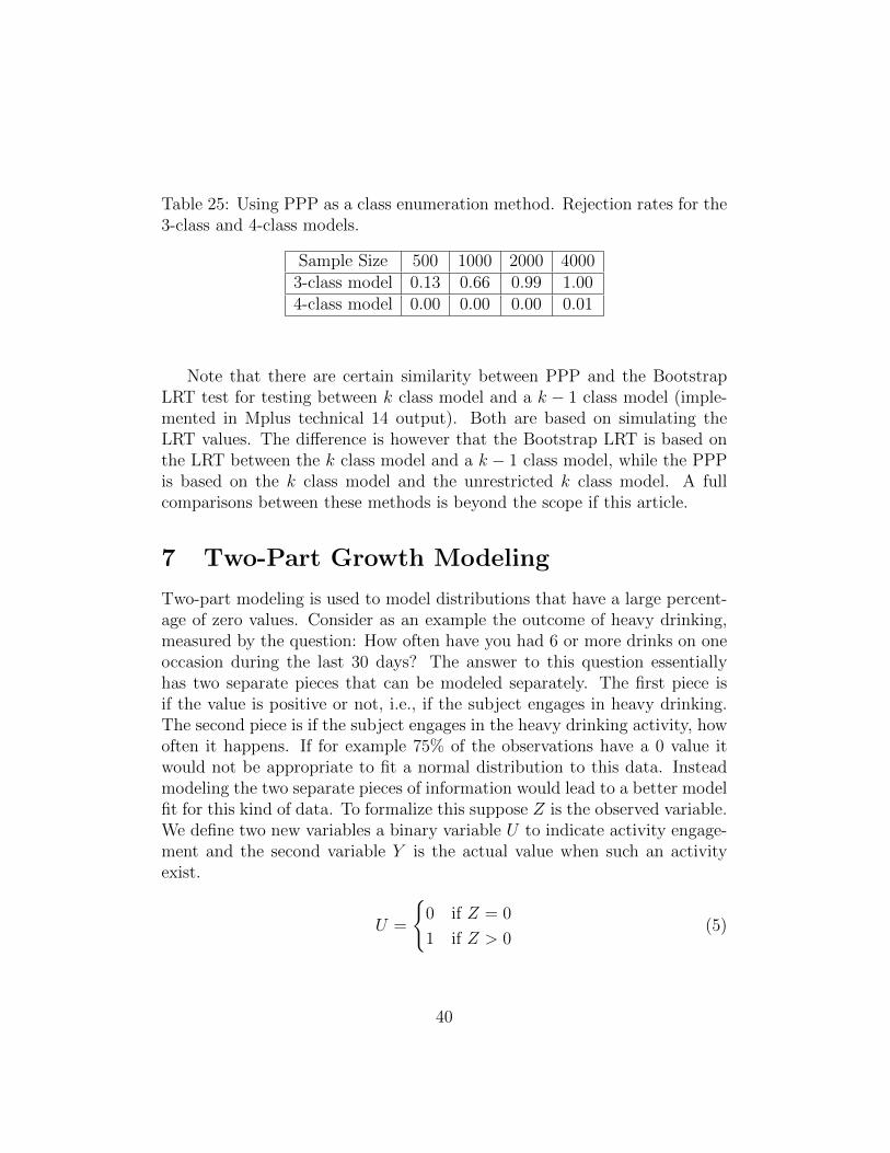
Table 25: Using PPP as a class enumeration method. Rejection rates for the3-class and 4-class models.

Sample Size 500 1000 2000 40003-class model 0.13 0.66 0.99 1.004-class model 0.00 0.00 0.00 0.01

Note that there are certain similarity between PPP and the BootstrapLRT test for testing between k class model and a k − 1 class model (imple-mented in Mplus technical 14 output). Both are based on simulating theLRT values. The difference is however that the Bootstrap LRT is based onthe LRT between the k class model and a k − 1 class model, while the PPPis based on the k class model and the unrestricted k class model. A fullcomparisons between these methods is beyond the scope if this article.

7 Two-Part Growth Modeling

Two-part modeling is used to model distributions that have a large percent-age of zero values. Consider as an example the outcome of heavy drinking,measured by the question: How often have you had 6 or more drinks on oneoccasion during the last 30 days? The answer to this question essentiallyhas two separate pieces that can be modeled separately. The first piece isif the value is positive or not, i.e., if the subject engages in heavy drinking.The second piece is if the subject engages in the heavy drinking activity, howoften it happens. If for example 75% of the observations have a 0 value itwould not be appropriate to fit a normal distribution to this data. Insteadmodeling the two separate pieces of information would lead to a better modelfit for this kind of data. To formalize this suppose Z is the observed variable.We define two new variables a binary variable U to indicate activity engage-ment and the second variable Y is the actual value when such an activityexist.

U =

{0 if Z = 0

1 if Z > 0(5)

40

Y =

{missing if Z = 0

Z if Z > 0(6)

At this point one can use standard models such as logistic or probit regres-sion for U and linear regression for Y to construct elaborate models. Formore information on two-part modeling see Olsen and Schafer (2001). Inlongitudinal settings we have multiple observations for the same individualand thus we can estimate a growth model for the U variables as well as theY variables. Typically the random effects in the two growth models are cor-related and therefore we estimate a joint model for U and Y . Because themissing values for Y are directly predicted by the U variables we have a MARsituation, that is, not MCAR. This means that the WLSMV estimator is notappropriate. The WLSMV estimates for this model are usually very biasedand thus we will not include the WLSMV estimator in this discussion. TheML estimates are unbiased however numerical integration is required. In theexample that we describe below we use a quadratic growth model for the Uvariables which means that the numerical integration is 3 dimensional, whichis feasible but can be quite slow. Thus the Bayes estimator is of interest as apotentially more computationally efficient estimator. Another reason to usethe Bayes estimator for this model is the fact that it provides a model fitthrough the PPP value. Such model fit is not available for the ML estimator.The PPP value essentially will compare the two-part model against an unre-stricted variance covariance matrix for all Y and U∗ variables thus it will beuseful in evaluating the fit of the growth curves. It is not possible to estimatethe same unrestricted model with the ML estimator because it typically leadsto high dimensional numerical integration which is not feasible.

In this section we conduct a simulation study based on the two-partgrowth example presented in Muthen (2010). There are 5 repeated measuresfor each individual and there are 1192 individuals in the sample. Both theU part of the model and the Y part of the model are fitted to a quadraticgrowth curve. The model can be described as follows.

P (Uij = 1) = Φ(η1i + η2itj + η3it2j)

Yij = η4i + η5itj + η6it2j + εij

The random effects η1i, ..., η6i are estimated as correlated random effects withmean α and variance covariance Ψ. These parameters amount to 27 param-eters, in addition we have the 5 residual variance parameters θj for εij so in

41

total the model has 32 parameters. To generate data we use the parametervalues reported in Muthen (2010) with one exception. The variance param-eter ψ66 was estimated as 0.02. As it was explained in Section 5.2 such avalue should be interpreted as 0 in Bayes estimation. Thus we generate thedata using ψ6k = 0 for k = 1, .., 6 and analyze the data with the same model,where these parameters are fixed to 0, i.e., the quadratic effect is a fixedeffect for the Y part of the model. Eliminating the 6 Ψ parameters we geta model with 26 parameters. Here we describe the simulation study basedon this model. We also conducted a simulation study with the small ψ6k

values however the Bayes estimator will always push the values away fromzero and that creates bias not just for the variance parameter but also forother parameters in the model. The most appropriate approach is to elimi-nate small variance random effects and convert them into fixed effects. If thesmall variance random effect is considered important the time score variablestj can be rescaled (for example they can be divided by a factor of 2) so thatvariance parameter is estimated to a larger value.

In the simulation study we use the Mplus default Inverse-Wishart priorIW(I,6) for the variance covariance matrix Ψ, see Appendix A. Using thisprior is important. As we have seen previously for models that are somewhatdifficult to identify the priors can have an effect on the results even when thesample size is large. For this example using for example the prior of IW(0,-6) leads to worse estimates and coverage. The prior for the α parametersis uniform on (−∞,∞), with the exception of α1 which is estimated as athreshold parameter with prior N(0, 5). The prior for the θ parameters isIG(−1, 0). These priors are all Mplus defaults and they have little influenceon the estimates because the sample size is not small. The results of thesimulation study for the Bayes and the ML estimator are presented in Table26. The computational time for the ML estimator is 6 times as much asthat for the Bayes estimator (2 minutes per replication v.s. 20 seconds perreplication). The convergence rate for the Bayes estimator is 100% while forML it is 95%. Both the Bayes estimator and the ML estimator produce smallbias and good coverage. The bias of the Bayes estimates is slightly bigger andfor some of the parameter the coverage drops down to 77% however. Since themodel is somewhat difficult to identify (for example here 3 random effectsare identified from 5 binary variables) we can assume that if the MCMCsequence is run longer the results will improve. The PPP value did not rejectthe model, i.e., the model was accepted in every replication in the simulationstudy. On the other hand when we analyze the same data but using only a

42

linear growth model rather than a quadratic in both the U and the Y partsof the model then the model is rejected 100% of the time. Therefore the PPPcan indeed be used as a test of fit for the two-part model. This feature isvery valuable alone in the absence of any other alternatives.

43

Table 26: Absolute bias(percent coverage) for two-part model

Parameter True Value ML Bayesα1 -0.81 0.01(93) 0.00(96)α2 -0.68 0.00(95) 0.11(89)α3 -0.31 0.00(96) 0.06(77)α4 0.42 0.00(95) 0.00(95)α5 -0.16 0.00(92) 0.02(91)α6 -0.09 0.00(94) 0.00(92)ψ11 4.11 0.06(98) 0.02(96)ψ22 3.03 0.09(96) 0.26(91)ψ33 0.33 0.01(96) 0.08(83)ψ44 0.22 0.00(98) 0.00(97)ψ55 0.18 0.00(93) 0.00(96)ψ21 1.96 0.03(97) 0.15(96)ψ31 0.54 0.01(97) 0.10(92)ψ32 0.94 0.03(97) 0.13(90)ψ41 0.72 0.02(97) 0.01(96)ψ42 0.31 0.00(97) 0.04(97)ψ43 0.09 0.00(98) 0.02(92)ψ51 -0.01 0.01(95) 0.02(93)ψ52 0.33 0.00(97) 0.00(94)ψ53 0.10 0.00(99) 0.00(95)ψ54 0.06 0.00(94) 0.00(95)θ1 0.10 0.00(92) 0.00(91)θ2 0.20 0.00(94) 0.00(97)θ3 0.21 0.00(95) 0.00(94)θ4 0.19 0.00(98) 0.00(96)θ5 0.18 0.00(91) 0.00(92)

44

8 Multiple Indicator Growth Modeling for Cat-

egorical Variables. Comparing the Efficiency

of the Bayes and the WSLMV Estimators.

In this section we simply demonstrate the quality of the Bayes estimationwhen there is a large number of factors and a large number of categoricalindicators. If there is missing data the WLSMV estimator could be inap-propriate because the missing data could be MAR and only full informationestimation methods such as the Bayes and the ML estimators are appropri-ate. Another reason for preferring a full information method is the fact thatfull information methods are asymptotically the most efficient, i.e., yield theminimal mean squared error MSE. When the number of indicators is largehowever the ML estimator is not computationally feasible if the factors aremeasured by categorical variables because that leads to numerical integra-tion that is extremely heavy computationally with 4 or more factors. It ispossible to use Montecarlo integration methods for such models to obtain theML estimates however that method is somewhat more difficult to conduct.It suffers from frequent non-convergence problems due to the fact that esti-mates for the log-likelihood can contain substantial error which will leads todifficulty in maximizing the log-likelihood. Typically the EM algorithm usedfor the ML estimation produces monotonically increasing likelihood whichenables us to easily monitor convergence. With the Montecarlo integrationhowever that happens only for certain parameterizations. In general the in-tegration error will results in a non-monotonic log-likelihood which becomesa problem in evaluating the convergence.

In this section we use as an example the multiple indicator growth modeldescribed in Muthen (2010). This example combines IRT and growth mod-eling using nine binary indicators of a factor measured at eight time points.The ML estimation requires eight dimensions of integration and thus it isnot feasible. We use the parameter values reported in Muthen (2010) toconstruct a simulation study. We generate 100 data sets and analyze themwith the Bayes and the WLSMV estimators. The sample size in the originalexample is 1174 and we generate all data sets to be of that size. The modelcan be described as follows. For t = 1, ..., 8; j = 1, ..., 9; k = 0, 1, 2 andi = 1, ..., 1174

P (Uijt = 1) = Φ(νj + λjηit)

45

ηit = ζ0i + ζ1it+ ζ2it2 + εit.

ζki = αk + βkWi + ξik.

where all of the latent variables ηit, ζki, εit, and ξik are normally distributedand Wi is a binary covariate. For identification λ1 = 1 and α0 = 0. Thefree parameters in the model are the 9 parameters νj, the 8 parameters λj, the 8 residual variances θt of εit, the 2 parameters αk, the 3 parametersβk, and the 6 parameters in the multivariate N(0,Ψ) distribution of ξik fora total of 36 parameters. The variance ψ22 is estimated to a value near 0in the original example so we are going to again fix the quadratic randomeffect to 0, essentially eliminating the 3 parameters ψk2, i.e., the model has33 parameters and this is the model we use for generating the data and themodel we estimate. As described in the above equations the time of theobservations are 1,...,8, however, that is not quite accurate. The actual 8times of observations that are used for this model are 0, .5, 1.5, 2.5, 3.5,4.5, 5.5, 6.5. To avoid having decimal point in the indices we abuse thenotation here. For the Bayes estimation we use the following priors. Forthe Ψ matrix we use the inverse-wishart prior IW (I, 3), for the parametersθt we use the inverse-gamma prior IG(−1, 0), for the νj and λj parameterswe use the normal N(0, 5) prior and for αk and βk we use the uniform prioron (−∞,∞). The results of the simulation study are presented in Table27. Both estimators yield unbiased estimates and confidence interval cov-erage near the 95% nominal level. The Bayes estimates yield smaller MSEthan the WLSMV estimates for most parameters, i.e., the Bayes estimatescan be considered more accurate than the WLSMV estimates. This con-firms the well known theoretical results that full information methods areasymptotically most efficient. Note that the Bayes and the ML estimator areasymptotically equivalent. In addition the PPP value accepted the model100% of the time while the WLSMV estimator accepted the model 93% ofthe time. The computational time for the Bayes estimator is about 1.5 timesthe computational time for the WLSMV estimator (2.5 v.s. 3.5 minutes perreplication). The convergence criteria used with the Bayes estimator is theautomated PSR convergence criterion implemented in Mplus. We concludethat the Bayes estimator provides a valid full-information alternative to theWLSMV estimator and can be used for example to ensure that missing datais properly accounted for or to ensure that the most efficient estimates areobtained.

46

Table 27: Absolute bias(percent coverage) for multiple indicator growthmodel

Parameter True Value WLSMV Bayes WLSMV-MSE / Bayes-MSEν1 0.39 0.00(94) 0.01(86) 1.21ν2 0.2 0.00(94) 0.00(85) 1.32ν3 -1.66 0.02(92) 0.00(89) 1.38ν4 -1.81 0.02(96) 0.01(92) 1.63ν5 -0.39 0.00(92) 0.00(88) 1.43ν6 -1.35 0.01(93) 0.00(90) 1.78ν7 -0.83 0.00(92) 0.00(88) 1.38ν8 -0.67 0.01(98) 0.00(85) 1.33ν9 -0.05 0.00(92) 0.00(89) 1.19λ2 1.40 0.00(97) 0.02(88) 1.22λ3 1.89 0.01(95) 0.03(85) 1.69λ4 1.34 0.01(96) 0.02(90) 1.62λ5 1.18 0.00(94) 0.02(84) 1.23λ6 1.42 0.01(92) 0.02(92) 1.94λ7 1.42 0.00(96) 0.02(89) 1.26λ8 1.32 0.01(93) 0.02(91) 1.67λ9 1.29 0.01(96) 0.01(91) 1.24θ1 0.15 0.01(96) 0.02(92) 1.36θ2 0.49 0.02(94) 0.02(93) 1.82θ3 1.72 0.04(97) 0.06(94) 1.97θ4 0.87 0.02(97) 0.01(94) 1.66θ5 0.69 0.00(94) 0.01(95) 2.22θ6 0.75 0.01(92) 0.04(90) 1.67θ7 0.96 0.01(98) 0.09(87) 0.81θ8 0.53 0.02(94) 0.07(84) 1.20α1 0.00 0.00(97) 0.00(92) 0.91α2 0.00 0.00(92) 0.00(94) 1.00β0 0.62 0.01(97) 0.00(88) 0.88β1 0.11 0.00(100) 0.00(90) 0.75β2 -0.02 0.00(96) 0.00(91) 1.00ψ11 1.77 0.05(93) 0.05(93) 1.81ψ22 0.25 0.01(93) 0.01(93) 1.25ψ21 -0.41 0.01(92) 0.01(91) 1.83

47

9 Multiple Indicator Two-level Growth Mod-

eling for Categorical Variables

In this section we present the two-level version of the multiple indicatorgrowth model described in the previous section. Our goal is to demonstratethe quality of the Bayes estimation for such complex models and to describea PX parameterization that can be useful for the estimation of these growthmodels. We describe a simulation study based on a model similar to themultiple indicator growth model example described in Muthen (2010). Inthis simulation there 100 clusters with 30 observations in each cluster. Theobserved variables are ordered polytomous variables with 6 observed valuesrather than binary indicators. The dependent variables are again observedat 8 different time points. At each time point three ordered polytomous vari-ables are observed. At each time point the three observed variables measurea single continuous factor. The eight continuous factors are decomposed asbetween-within variables and a linear growth model is fitted separately forthe within and the between parts. Let Uijkt be the j−th observed variable forobservation i in cluster k at time t. The model is described by the followingequations

Uijkt = l⇔ τj,l−1 < U∗ijkt ≤ τj,l

U∗ijkt = λjηikt + εijkt

ηikt = ηikt,w + ηkt,b

ηikt,w = ζ0ik,w + ζ1ik,wt+ εikt,w

ηkt,b = ζ0k,b + ζ1k,bt+ εkt,b

ζrik,w = βr,wWik + ξrik,w

ζrk,b = αr,b + ξrk,b

where the indices vary as follows k = 1, ..., 100, i = 1, ...30, j = 1, ..., 3, r =0, 1, t = 1, ..., 8, and l = 1, ..., 6. In addition the index w indicates that thevariable is defined on the within/individual level while the index b indicatesthat the variable is defined on the between/cluster level. The variable Wik isan observed covariate on the individual level. All other variables are latentnormally distributed variables in this model.

Let’s now identify all the parameters in this model. There are 15 thresh-old parameters τj,l, for j = 1, ...3 and l = 1, ..., 5; two loading parameters

48

λj where j = 2, 3. Note that the first loading parameter is fixed to 1 foridentification purposes. There are two parameters βr,w for r = 0, 1. For iden-tification purposes α0,b is fixed to 0 but the parameter α1,b is estimated. Foridentification purposes the residual variance of εijkt is fixed to 1. There are8 within level residual variance parameters θw,t = V ar(εikt,w) and 8 betweenlevel residual variance parameters θb,t = V ar(εkt,b). Finally we have 3 pa-rameters Ψw describing the variance covariance of the within level interceptand slope ξ0ik,w and ξ1ik,w and also 3 parameters Ψb describing the variancecovariance of the between level intercept and slope ξ0k,b and ξ1k,b. In totalwe have 42 parameters.

The parameter extended (PX) parameterization estimates just one moreparameter, that is the parameter α0,b. Adding this parameter to the modelwe essentially make all threshold parameters unidentified. To be able tointerpret the estimated model with this parameterization we have to use thestandardized threshold parameters τ sj,l in place of the threshold parametersτj,l, where the standardized parameters are obtained from

τ sj,l = τj,l − α0,b.

The goal of this simulation study is to demonstrate the advantage of thePX parameterization with the Bayes estimator. In principle this model canbe estimated with the WLSMV estimator in Mplus, however that estimatorhas the same disadvantages that were demonstrated in the previous sections.It does not support optimal treatment of missing data, i.e., it doesn’t sup-port MAR. In addition the WLSMV estimator is less efficient than the fullinformation Bayes estimator. The ML estimator is not feasible for this modelas it would require 16 dimensions of integration.

In this simulation study we generate 50 samples and analyze them withboth the standard parameterization and with the PX parameterization. Inall analysis 40000 MCMC iterations have been performed. The results arepresented in Table 28. Both estimation procedures perform well howeverwith the regular parameterization some of the parameters have low coverageand somewhat bigger bias. From these simulation results we conclude thatthe PX parameterization is useful in improving the mixing in the Bayesestimation. It is worth noting also that when we used binary indicators thePX procedure was not needed. This is because for binary items the thresholdparameters are estimated as means for the underlying latent variables. Thisway one of several highly correlated components in the Gibbs sampler is

49

eliminated. When the indicator variables however are not binary but orderedpolythomous this is not possible. The PX parameterizations appears to besuccessfully resolving the problem of highly correlated components in theGibbs sampler. Using the regular parameterization it is possible to obtainthe same quality results as the PX parameterization but it will simply requirea much larger number of MCMC iterations.

50

Table 28: Absolute bias(coverage) for two-level growth model

Parameter True Value Bayes Bayes-PXτ1,1 1.88 0.07(0.84) 0.02(0.96)τ1,2 3.33 0.06(0.86) 0.03(0.94)τ1,3 4.36 0.06(0.84) 0.03(0.92)τ1,4 4.91 0.05(0.88) 0.04(0.94)τ1,5 5.62 0.05(0.86) 0.04(0.94)τ2,1 1.10 0.08(0.80) 0.00(0.96)τ2,2 2.38 0.08(0.82) 0.00(0.96)τ2,3 3.40 0.08(0.82) 0.00(0.96)τ2,4 3.97 0.09(0.86) 0.00(0.92)τ2,5 4.85 0.08(0.88) 0.00(0.96)τ3,1 1.13 0.08(0.82) 0.00(0.96)τ3,2 2.40 0.08(0.78) 0.00(0.96)τ3,3 3.32 0.09(0.78) 0.00(0.94)τ3,4 3.85 0.08(0.86) 0.00(0.96)τ3,5 4.58 0.09(0.84) 0.00(0.94)θw,1 0.78 0.02(0.94) 0.02(0.94)θw,2 0.28 0.01(0.98) 0.01(0.98)θw,3 1.48 0.01(0.94) 0.01(0.94)θw,4 2.48 0.05(0.90) 0.06(0.90)θw,5 2.07 0.06(0.90) 0.06(0.94)θw,6 1.69 0.03(0.98) 0.03(0.98)θw,7 1.80 0.04(0.92) 0.04(0.90)θw,8 2.13 0.08(1.00) 0.06(0.98)θb,1 1.04 0.06(0.92) 0.06(0.92)θb,2 0.92 0.08(0.92) 0.08(0.92)θb,3 1.30 0.08(0.94) 0.08(0.94)θb,4 0.28 0.02(0.98) 0.02(0.98)θb,5 0.16 0.01(0.92) 0.01(0.92)θb,6 0.18 0.00(0.94) 0.00(0.94)θb,7 0.36 0.01(0.92) 0.01(0.94)θb,8 0.07 0.03(0.94) 0.03(0.94)ψw,1,1 2.08 0.02(0.94) 0.03(0.96)ψw,2,2 0.05 0.00(0.94) 0.00(0.96)ψw,1,2 -0.17 0.00(1.00) 0.00(1.00)ψb,1,1 0.50 0.08(0.96) 0.06(0.96)ψb,2,2 0.02 0.00(0.94) 0.00(0.98)ψb,1,2 -0.05 0.01(0.94) 0.00(0.92)β0,w 1.18 0.02(0.94) 0.00(0.92)β1,w 0.03 0.00(0.96) 0.00(0.98)α1,b -0.10 0.02(0.86) 0.00(0.94)λ2 0.90 0.01(0.92) 0.01(0.90)λ3 0.88 0.01(0.96) 0.01(0.88)

51

10 Appendix A. Priors

Choosing meaningful priors is important when the estimates and the pos-terior distribution show ”prior dependence”. In addition when informativepriors are available it is important to specify these priors correctly. In thissection we provide a brief tutorial for how to set up the Inverse Gamma andInverse Wishart priors.

10.1 Inverse Gamma Prior

The inverse gamma prior IG(α, β) has a positive density on (0,∞). Figures1-6 show some examples of inverse gamma density function. The densityfunction is given by

βα

Γ(α)x−α−1Exp(−β/X)

where Γ is the gamma function. The mean of the distribution is

β

α− 1

when α > 1, otherwise it is infinity. The variance of the distribution is

β2

(α− 1)2(α− 2)

when α > 2, otherwise it infinity. To set up an informative conjugate inversegamma prior for a variance parameter one can simply solve the system ofequations for α and β

m =β

α− 1

v =β2

(α− 1)2(α− 2)

where m and v are the mean and the variance of the informative prior.Fortunately this system is very easy to solve.

α = 2 +m2

v

β = m+m3

v

52

Figure 1: IG(1, 1) density

0 0.5 1 1.5 2 2.5 3 3.5 4 4.5 50

0.1

0.2

0.3

0.4

0.5

0.6

0.7

When α is small and the variance or the mean is infinity it is useful toconsider the mode of the distribution

β

α + 1.

The parameter β is a scale parameter for the inverse gamma distribution.Thus if X ∼ IG(α, 1) then βX ∼ IG(α, β). For this distribution to beproper both parameters α and β should be positive. The Mplus default ofIG(−1, 0) is basically the uniform prior on (0,∞). Another prior that isfrequently used as uninformative prior is the IG(0, 0). This is an improperprior with density 1/x and for practical purposes it can be thought as IG(ε, ε)where ε is very small positive number. The density curve of IG(0, 0) can bevisualized by approximating it with the density of IG(0.001, 0.001).

53

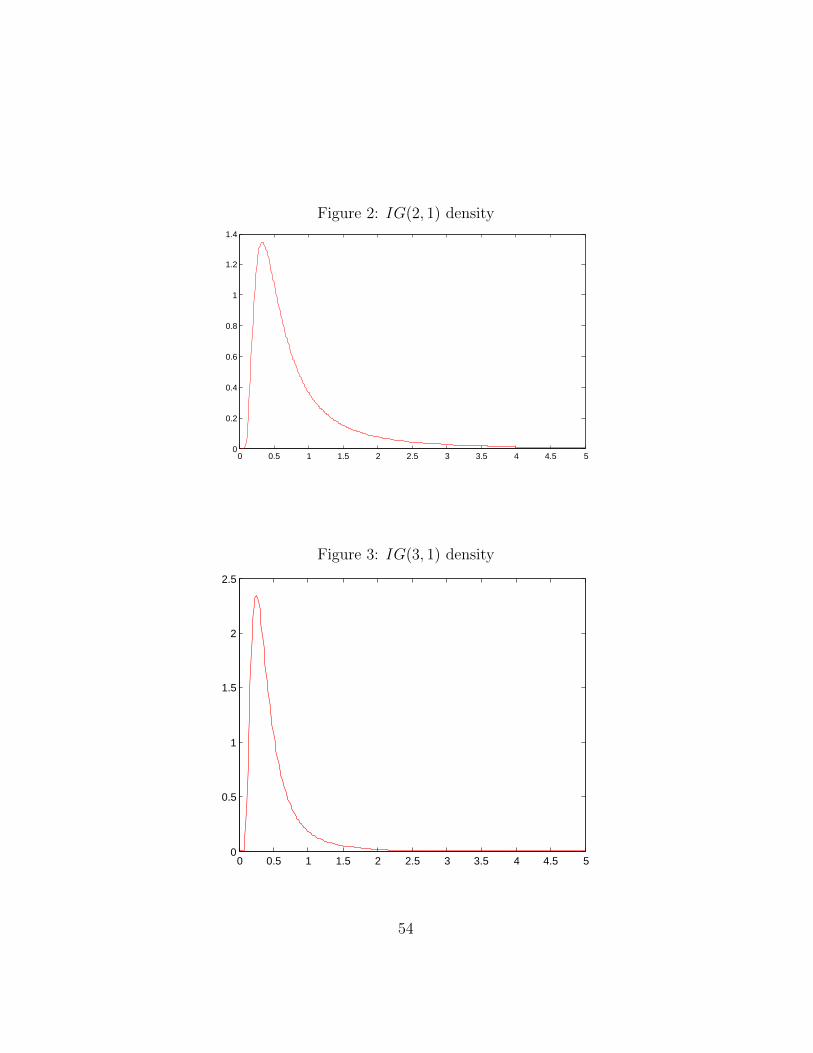
Figure 2: IG(2, 1) density

0 0.5 1 1.5 2 2.5 3 3.5 4 4.5 50

0.2

0.4

0.6

0.8

1

1.2

1.4

Figure 3: IG(3, 1) density

0 0.5 1 1.5 2 2.5 3 3.5 4 4.5 50

0.5

1

1.5

2

2.5

54

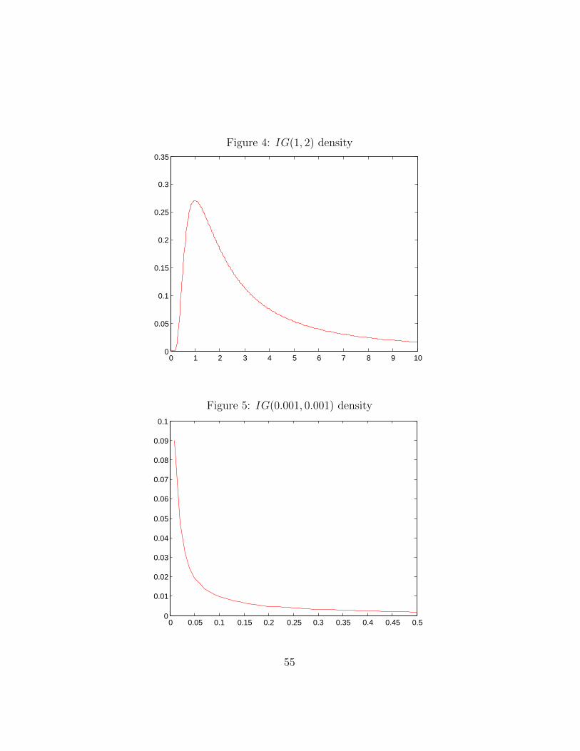
Figure 4: IG(1, 2) density

0 1 2 3 4 5 6 7 8 9 100

0.05

0.1

0.15

0.2

0.25

0.3

0.35

Figure 5: IG(0.001, 0.001) density

0 0.05 0.1 0.15 0.2 0.25 0.3 0.35 0.4 0.45 0.50

0.01

0.02

0.03

0.04

0.05

0.06

0.07

0.08

0.09

0.1

55

Figure 6: IG(0.5, 1) density

0 1 2 3 4 5 6 7 8 9 100

0.05

0.1

0.15

0.2

0.25

10.2 Inverse Wishart Distribution

The domain of the Inverse Wishart distribution IW (Ψ,m) is all positivedefinite matrices of size p. The density is given by

|Ψ|m/2|X|−(m+p+1)/2Exp(−Tr(ΨX−1)/2)

2mp/2Γp(m/2)

where Γp is the multivariate gamma function and the argument X of thedensity is a positive density function. To set informative prior with certainexpected value we can use the fact that the mean of the distribution is

Ψ

m− p− 1.

The mean exists and is finite only if m > p + 1. If m ≤ p + 1 then we canuse the fact that the mode of the distribution is

Ψ

m+ p+ 1.

The variance, i.e., the level of informativeness is controlled exclusively by theparameter m. The larger the value of m the more informative the prior is.

56

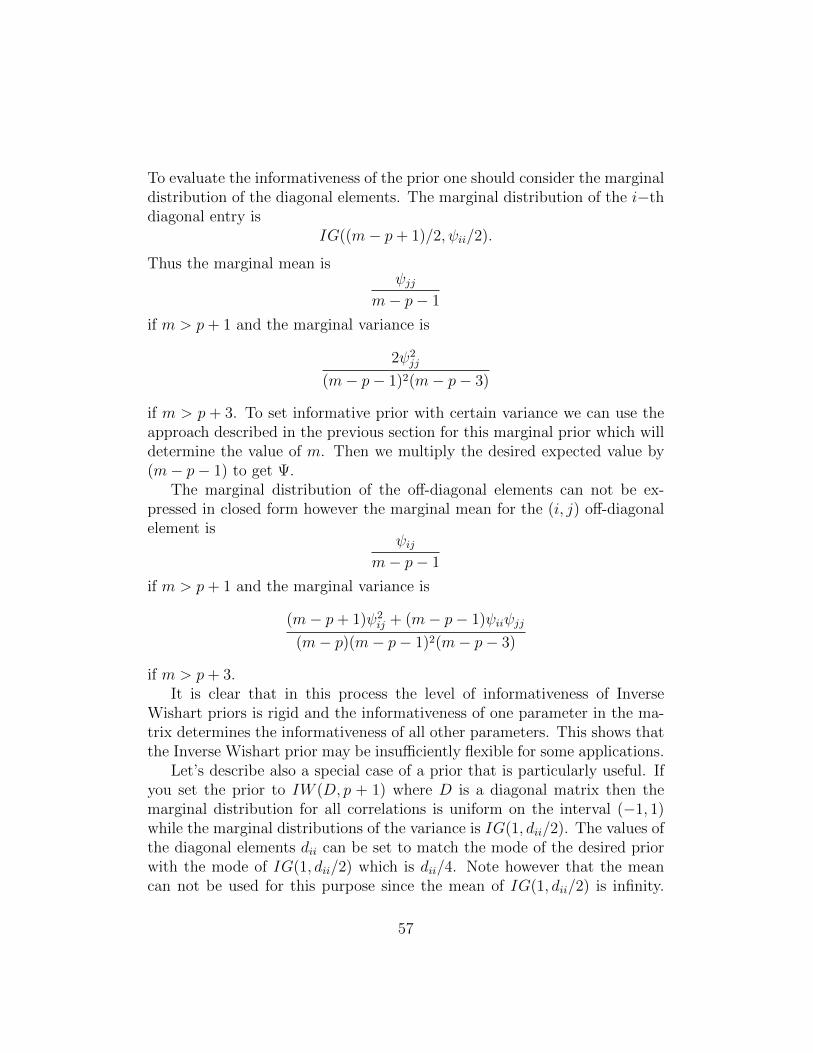
To evaluate the informativeness of the prior one should consider the marginaldistribution of the diagonal elements. The marginal distribution of the i−thdiagonal entry is

IG((m− p+ 1)/2, ψii/2).

Thus the marginal mean isψjj

m− p− 1

if m > p+ 1 and the marginal variance is

2ψ2jj

(m− p− 1)2(m− p− 3)

if m > p + 3. To set informative prior with certain variance we can use theapproach described in the previous section for this marginal prior which willdetermine the value of m. Then we multiply the desired expected value by(m− p− 1) to get Ψ.

The marginal distribution of the off-diagonal elements can not be ex-pressed in closed form however the marginal mean for the (i, j) off-diagonalelement is

ψijm− p− 1

if m > p+ 1 and the marginal variance is

(m− p+ 1)ψ2ij + (m− p− 1)ψiiψjj

(m− p)(m− p− 1)2(m− p− 3)

if m > p+ 3.It is clear that in this process the level of informativeness of Inverse

Wishart priors is rigid and the informativeness of one parameter in the ma-trix determines the informativeness of all other parameters. This shows thatthe Inverse Wishart prior may be insufficiently flexible for some applications.

Let’s describe also a special case of a prior that is particularly useful. Ifyou set the prior to IW (D, p + 1) where D is a diagonal matrix then themarginal distribution for all correlations is uniform on the interval (−1, 1)while the marginal distributions of the variance is IG(1, dii/2). The values ofthe diagonal elements dii can be set to match the mode of the desired priorwith the mode of IG(1, dii/2) which is dii/4. Note however that the meancan not be used for this purpose since the mean of IG(1, dii/2) is infinity.

57

Only the mode is defined for this distribution. In this case the marginaldistribution of the diagonal elements has infinite mean and variance. Themarginal for the covariance elements has mean zero by symmetry but alsohas an infinite variance. The marginal mean for the correlation parameter iszero and the marginal variance for the correlation parameter is 1/3.

More generally setting the prior to IW (D,m) where D is a diagonalmatrix, the marginal distribution for all correlations is the beta distributionB((m− p + 1)/2, (m− p + 1)/2) on the interval (-1,1), if m ≥ p with mean0 and variance

1

m− p+ 2.

Note also that the posterior distribution in the MCMC generation for thevariance covariance parameter with prior IW (Ψ,m) is a weighted averageof Ψ/m and the sample variance where the weights are m/(n + m) andn/(n + m) respectively, where n is the sample size. Thus one can interpretthe degrees of freedom parameter m as the number of observations addedto the sample with the prior variance covariance matrix. Naturally as thesample size increases the weight m/(n+m) will converge to 0 and the effectof the prior matrix Ψ will diminish. The maintain the same effect of the prioron the estimation for larger sample sizes the degrees of freedom parametershould be chosen proportionally larger.

More information on the Inverse Wishart distribution and the marginaldistributions of all the entries in the matrix can be found in Barnard et al.(2000).

10.3 Default Priors

In this section we describe the default priors used in Mplus. The defaultprior for intercepts, regression slopes, and loading parameters is N(0,∞),unless these parameters are directly in a probit regression and in that casethe default is N(0, 5). The default for variance parameters, i.e., variancecovariance blocks of size 1 is IG(0,−1). The default for variance covarianceblocks of size bigger than 1 is IW (0,−p−1), where p is the size of the matrix,unless the variance covariance matrix also includes parameters from a probitregression, and in that case the default is IW (I, p + 1). For unrestrictedmodel imputation even when all variables are continuous the default prior isIW (I, p + 1). The default priors for threshold parameters is N(0,∞). Thedefault prior for all class proportions is the Dirichlet prior D(10, 10, ..., 10).

58

References

[1] Asparouhov, T. and Muthen, B. (2010) Bayesian Analysis Us-ing Mplus: Technical Implementation. Mplus Technical Report.http:\\www.statmodel.com

[2] Barnard, J., McCulloch, R. E., and Meng, X. L. (2000). Modeling co-variance matrices in terms of standard deviations and correlations, withapplication to shrinkage. Statistica Sinica 10, 1281-1311.

[3] Browne, W. J., and Draper, D. (2006). A comparison of Bayesian andlikelihood-based methods for fitting multilevel models. Bayesian Analy-sis, 1, 473-514.

[4] Dunson D., Palomo J., and Bollen K. (2005) Bayesian struc- tural equa-tion modeling. SAMSI TR2005-5. http:\\www.samsi.info\TR\tr2005-05.pdf

[5] Fox, J.P., and Glas, C. A.W. (2001). Bayesian estimation of a multilevelIRT model using Gibbs sampling. Psychometrika, 66, 271-288.

[6] Gelman A. (2006) Prior distributions for variance parameters in hierar-chical models. Bayesian Analysis 1, 515-533.

[7] Gelman A., Jakulin A., Pittau M. G., Su Y. S. (2008a). A weakly infor-mative default prior distribution for logistic and other regression models.The Annals of Applied Statistics, 2, 1360-1383.

[8] Gelman A., van Dyk, D. A., Huang Z., Boscardin J. (2008b) UsingRedundant Parameterizations to Fit Hierarchical Models. Journal OfComputational And Graphical Statistics, 17, 95-122.

[9] Hjort, N. L., Dahl, F. A. and Steinbakk, G. H. (2006). Post-processingposterior predictive p-values. J. Amer. Statist. Assoc. 101, 1157-1174.

[10] Muthen, B. (2010) Bayesian Analysis In Mplus: A Brief Introduction.Mplus Technical Report. http:\\www.statmodel.com

[11] Muthen, B., Asparouhov, T., Hunter, A. & Leuchter, A. (2010). Growthmodeling with non-ignorable dropout: Alternative analyses of theSTAR*D antidepressant trial. Submitted for publication.

59

[12] Nylund, K. L., Asparouhov, T., & Muthn, B. O. (2007). Deciding on thenumber of classes in latent class analysis and growth mixture modeling:A Monte Carlo simulation. Structural Equation Modeling, 14, 535-569.

[13] Lee S. Y., Song X. Y., Cai J. H. (2010) A Bayesian Approach for Non-linear Structural Equation Models With Dichotomous Variables UsingLogit and Probit Links. Structural Equation Modeling, 17, 280-302.

[14] Olsen, M.K. & Schafer, J.L. (2001). A two-part random effects modelfor semicontinuous longitudinal data. Journal of the American StatisticalAssociation, 96, 730-745.

[15] Patz R. and Junker B. (1999) A Straightforward Approach to MarkovChain Monte Carlo Methods for Item Response Models Journal of Ed-ucational and Behavioral Statistics Summer, 24, 146-178.

[16] Raghunathan, T. E., Lepkowski, J. M., Van Hoewyk, J., and Solen-berger, P. (2001) A Multivariate Technique for Multiply Imputing Miss-ing Values Using a Sequence of Regression Models. Survey Methodology,Vol. 27, No 1. 85-95.

[17] Rubin, D.B. (1987) Multiple Imputation for Nonresponse in Surveys. J.Wiley & Sons, New York.

[18] Savalei, V. (2010) Small Sample Statistics for Incomplete NonnormalData: Extensions of Complete Data Formulae and a Monte Carlo Com-parison. Structural Equation Modeling, 17, 241-264.

[19] Segawa E., Emery S., and Curry S. (2008) Extended Generalized Lin-ear Latent and Mixed Model, Journal of Educational and BehavioralStatistics, 33, 464-484.

[20] Song X.Y., Xia Y. M., Lee S. Y. (2009) Bayesian semiparametric analy-sis of structural equation models with mixed continuous and unorderedcategorical variables. Statistics in Medicine, 28, 2253-2276.

[21] van Dyk, D. A., and Meng, X. L. (2001), The Art of Data Augmentation.Journal of Computational and Graphical Statistics, 10, 1-111.

60