Vincent Ho21 April 2008

Bayes' Theorem and its Application in Bayes' Theorem and its Application in Quantitative Risk AssessmentQuantitative Risk Assessment

(c. 1702 – 17 April 1761)

www.hkarms.org 2

Qualitative Definitions of Risk

• Risk is never zero by increasing level of safeguards, as long as hazard is present

SafeguardsHazardRisk =

• Without uncertainty or damage, there is no risk• Anybody can guess extent of damage with different

levels of uncertainties

DamageyUncertaintRisk ×=

• Classical, but most misleading. More useful in hazard analyses

eConsequencLikelihoodRisk ×=

www.hkarms.org 3

Sources of Uncertainties

• Impossible to explicitly enumerate all conditions• Inadequate or incorrect information on conditions• Inconsistent interpretation and classification of

events• Lack of success data (for number of demands and

exposure/mission time)• Limited data sample size; realised risk and

unrealised risk• Imperfect mathematical and computer modelling of

reality

www.hkarms.org 4

Uncertainties

• In general, there are three types of uncertainties associated with a risk assessment:– Stochastic uncertainties– Modelling uncertainties– Parametric uncertainties

• Strictly speaking, A+A≠2xA• It is this explicit consideration of uncertainties

distinguishes a risk assessment from a hazard analysis, a PRA from a “QRA”

• Uncertainties are measured by level of belief; i.e., probability

www.hkarms.org 5

Probability Functions

• The likelihood of an event E is indicated by Probability Function P(E)

• The sum of the probabilities of all elementary outcomes within sample space S, P(S) = 1, with values between 0 and 1– P(E) = 1: the event is CERTAIN to occur– P(E) = 0: the event is certain NOT to occur– Anything in between represents our level of belief of

the certainty or uncertainty of an event to occur

www.hkarms.org 6

The Laws of Probability

• The probability of any event A is 0 ≤ P(A) ≤ 1• Law of Addition: P(A ∪ B) = P(A) + P(B) - P(A ∩ B)

• Law of Multiplication: P(A ∩ B) = P(A) x P(B)

AA BB A and B

www.hkarms.org 7

Law of Multiplication

• Actually, P(A ∩ B) = P(B) x P(A|B)where P(A|B) is probability of A given B has occurred

• If A and B are statistically independent, – P(B|A) = P(B), then– P(A ∩ B) = P(A) x P(B|A) = P(A) P(B)

AAA

A∩BAA∩∩BB

BBB

www.hkarms.org 8

Bayes’ Theorem

• Bayes’ Theorem is a trivial consequence of the definition of conditional probability, but it is very useful in that it allows us to use one conditional probability to compute another

• Given that A and B are events in sample space S, and P(B) ≠ 0, conditional probability is defined as:– P(A ∩ B) = P(A|B) P(B)– P(A ∩ B) = P(B|A) P(A) – P(B|A) P(A) = P(A|B) P(B)

P(A)B)P(A

P(A)P(A|B)P(B)ABP ∩

==)|(

www.hkarms.org 9

Probability vs Frequency

• Frequency is a measure of the rate of occurrence. E.g., failure rate of a pump is 6.2x10-3/hr

• Probability is a measure of the level of belief, a fraction, or failure per demand. It is dimensionless. E.g., the failure rate of the pump is

Frequency Probability1.0x10-4/hr 0.22.0x10-3/hr 0.53.2x10-3/hr 0.24.5x10-2/hr 0.1

with a mean of 6.2x10-3/hr• The parameter failure rate is denoted as λ, and the

probability of the failure rate is P(λ = 1.0x10-4/hr) = 0.2

www.hkarms.org 10

Uncertainties Based on Evidence

• In general, two approaches to estimate parameters:– Frequentist

• Based only on observed data and an adopted model• Characterized by scientific objectivity

– Bayesian• Appropriately combining prior intuition or knowledge with

information from observed data• Characterized by subjective nature of prior opinion

• Each approach is valid when applied under specific circumstances

• Neither approach uniformly dominates the other

www.hkarms.org 11

Frequentist Statistics

• Relative frequency λ: proportion of times an outcome occurs

• For N→∞, the relative frequency tends to stabilize around some number: probability estimates

• Frequentist statistics will completely break down if no data or no experience history (N =0)– New technology– Rare events– No failure record

(N) trialsofnumberTotaltrialsuccessfulofNumber

=λ

www.hkarms.org 12

Bayesian Statistics

• Bayesian statistics measures degrees of belief by using intuition knowledge (prior belief), updating it by evidence (likelihood) to obtain a posterior belief P(B|A) = P(A|B)*P(B) / P(A)

• To process knowledgeP(Cause|Effect) = P(Effect|Cause) P(Cause) / P(Effect)

Posterior ∝ likelihood x prior

basically a normalizing constant

p (θj⏐data) = p (data⏐θj) p (θj) / Σ p (data⏐θi) p (θi)

www.hkarms.org 13

posterior probability, i.e., after seeing the data

prior probability, i.e.,before seeing the data

The likelihood of seeing evidence given prior

normalization involves summing over all possible hypotheses

Bayesian Statistics

• In a QRA, we know what the damage effects and their contributing factors are, we want to know the likelihood of the contributing factors

∫∞

=

0

)|()(

)|()()|('

λλπλ

λλπλπ

ELd

ELE

www.hkarms.org 14

How Many Defects in aPopulation of 100 Components?

www.hkarms.org 15

State of Knowledge after Various Samples

www.hkarms.org 16

State of Knowledge after Various Sample Results With Defects Found

www.hkarms.org 17

Typical Shapes of Probability Functions for Prior, Likelihood and Posterior

Prior

Likelihood

Posterior

www.hkarms.org 18

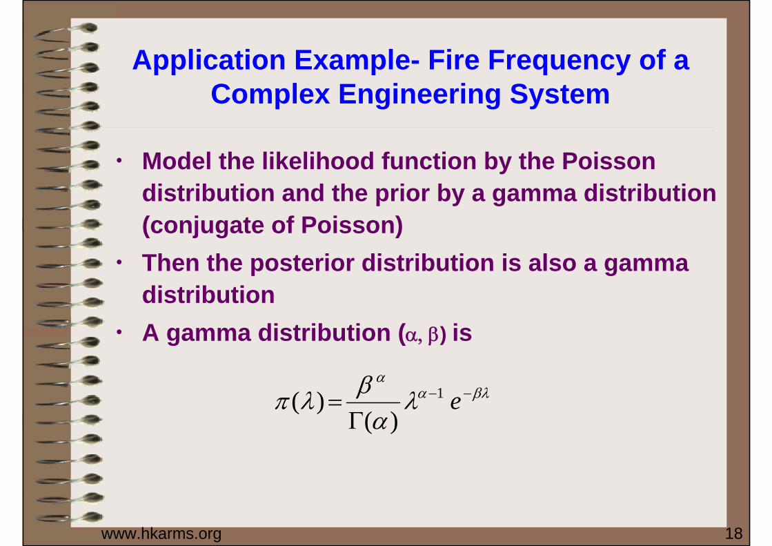
Application Example- Fire Frequency of a Complex Engineering System

• Model the likelihood function by the Poisson distribution and the prior by a gamma distribution (conjugate of Poisson)

• Then the posterior distribution is also a gamma distribution

• A gamma distribution (α, β) is

βλαα

λα

βλπ −−

Γ= e1

)()(

www.hkarms.org 19

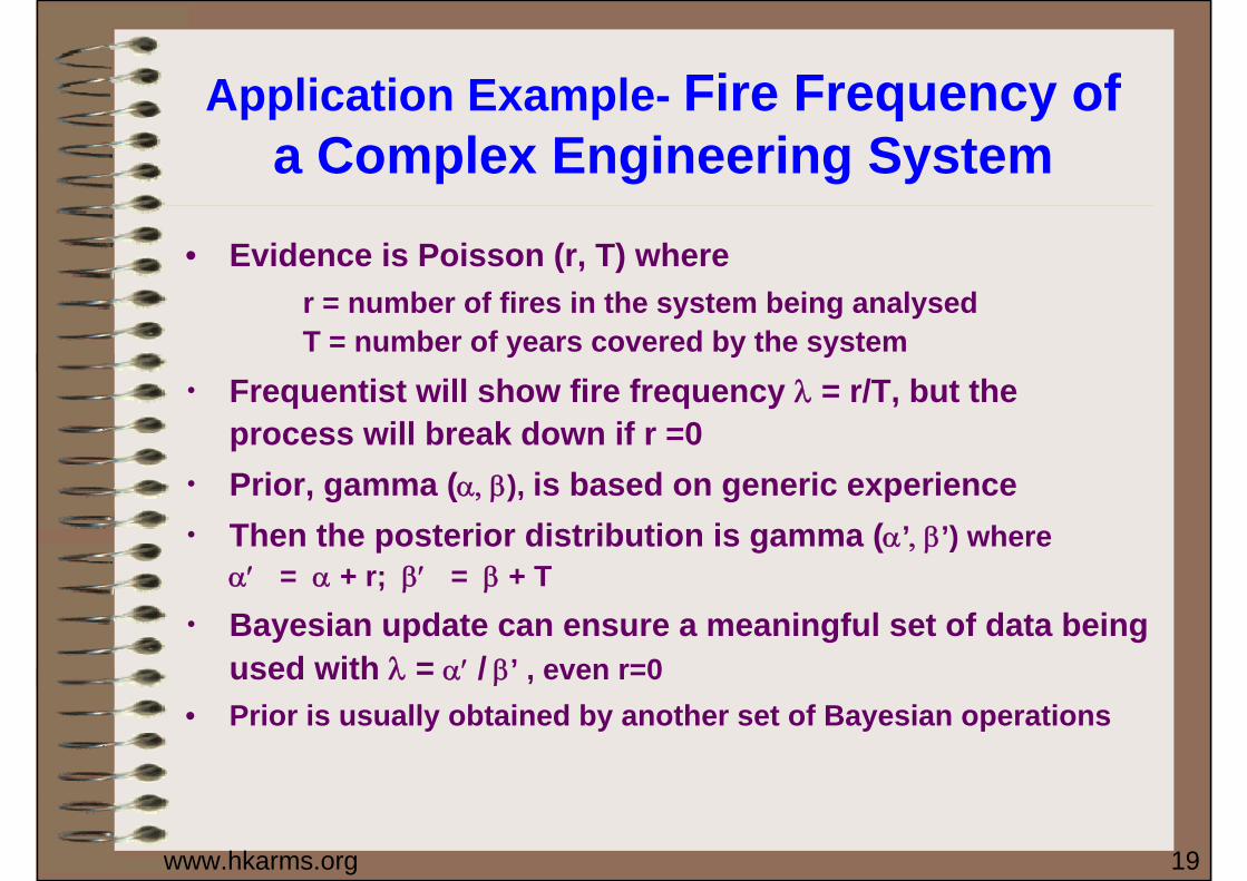
Application Example- Fire Frequency of a Complex Engineering System

• Evidence is Poisson (r, T) where r = number of fires in the system being analysedT = number of years covered by the system

• Frequentist will show fire frequency λ = r/T, but the process will break down if r =0

• Prior, gamma (α, β), is based on generic experience • Then the posterior distribution is gamma (α’, β’) where

α′ = α + r; β′ = β + T• Bayesian update can ensure a meaningful set of data being

used with λ = α′ / β’ , even r=0• Prior is usually obtained by another set of Bayesian operations

www.hkarms.org 20

Probability Curves for Fire Frequency (Example)

www.hkarms.org 21

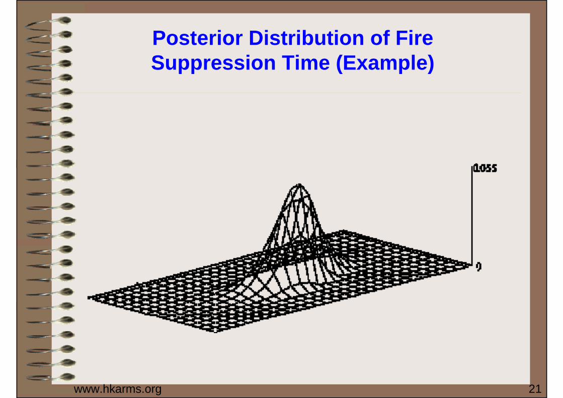
Posterior Distribution of Fire Suppression Time (Example)

www.hkarms.org 22

Properties of Bayesian Updating

• Need to estimate Prior and obtain the appropriate evidence– With weak evidence, prior dominates results– With strong evidence, results insensitive to prior

(dominated by evidence)– Successive updating gives same result as one-

step updating with consistent evidence• Provide a robust method in assessing

initializing event frequency, failure rates, event tree split fractions– Drawn on generic experience – Plant specific data (including no failure)

Probability of Impact….

End

www.psam9.org

Supplementary Notes(Advance Level)

www.hkarms.org 26

Bayes’ Theorem ExampleSuppose we have a new untested system. We estimate, based on prior experience, that 80% of chance the reliability (probability of successful run) R1 = 0.95, and 20% of chance that R2 = 0.75. We run a test and find that it operate successfully. What is the probability that the reliability level is R1.

Si = event “System test results in a success”

=0.8*0.95/(0.8*0.95 + 0.2*0.75) = 0.835 (updated from 0.8)

)R|P(S )P(R )R|P(S )P(R)R|P(S )P(R )S|P(R

212111

11111

+=

Now, let’s assume that a second test is also successful

=0.835*0.95/(0.835*0.95 + (1-0.835)*0.75) =0.79325/(0.79325+0.12375)=0.865

)R|P(S )P(R )R|P(S )P(R)R|P(S )P(R )S |P(R

222121

12121

+=

Mean = 0.95*0.8+0.75*0.2 = 0.91

0.20.75

0.80.95

PR

Prior Distribution

Mean = 0.917

1-0.835 = 0.1650.75

0.8350.95

PR

Posterior Distribution

Mean = 0.923

1-0.865 = 0.1350.75

0.8650.95

PR

2nd Posterior Distribution

What is P(R1|S3) if the S3 is a failure?

www.hkarms.org 27

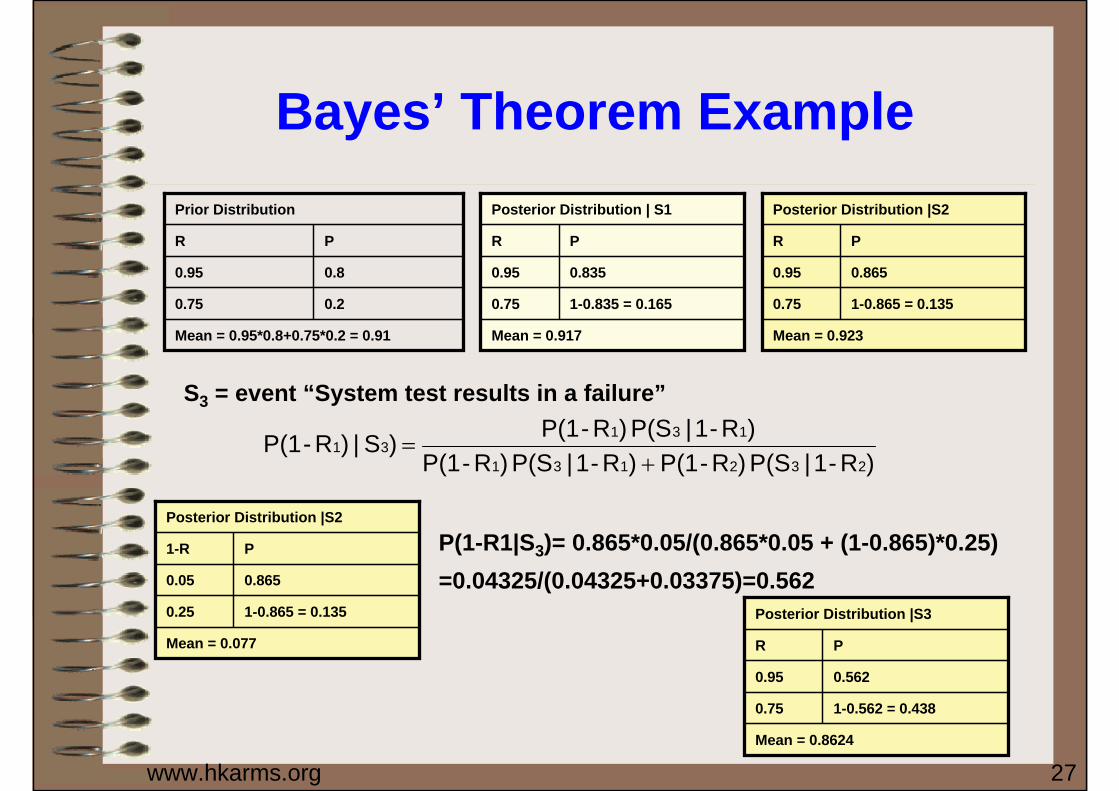
Bayes’ Theorem Example

S3 = event “System test results in a failure”

)R-1|P(S )R-P(1 )R-1|P(S )R-P(1)R-1|P(S )R-P(1 )S|)R-P(1

232131

13131

+=

P(1-R1|S3)= 0.865*0.05/(0.865*0.05 + (1-0.865)*0.25) =0.04325/(0.04325+0.03375)=0.562

Mean = 0.95*0.8+0.75*0.2 = 0.91

0.20.75

0.80.95

PR

Prior Distribution

Mean = 0.917

1-0.835 = 0.1650.75

0.8350.95

PR

Posterior Distribution | S1

Mean = 0.077

1-0.865 = 0.1350.25

0.8650.05

P1-R

Posterior Distribution |S2

Mean = 0.923

1-0.865 = 0.1350.75

0.8650.95

PR

Posterior Distribution |S2

Mean = 0.8624

1-0.562 = 0.4380.75

0.5620.95

PR

Posterior Distribution |S3

www.hkarms.org 28

Bayes’s theorem• Let us recall Bayes’s theorem:

• Where f(θ) is density of the prior probability distribution for parameter(s) of interest, f(x|θ) is density of conditional probability distribution for x given θ, f(θ|x) is posterior density of the distribution of the parameter of interest - θ. Integral is the normalisation coefficient that ensures that integral of posterior is equal to 1.

• Bayesian estimation is fundamentally different from the maximum likelihood estimation. In maximum likelihood estimation parameters we want to estimate are not random variables. In Bayesian statistics they are.

• Prior, likelihood and posterior have the following interpretations:• Prior: It reflects the state of our knowledge about the parameter(s) before

we have seen the data. E.g. if this distribution is sharp then we have fairly good idea about the parameter of interest.

• Likelihood: How likely it is to observe current observation if parameter of interest would have current value.

• Posterior: It reflects the state of our knowledge about the parameter(s) after we have observed (and treated) the data.

∫∞

∞−

=θθθ

θθθdxff

xffxf)|()(

)|()()|(

www.hkarms.org 29

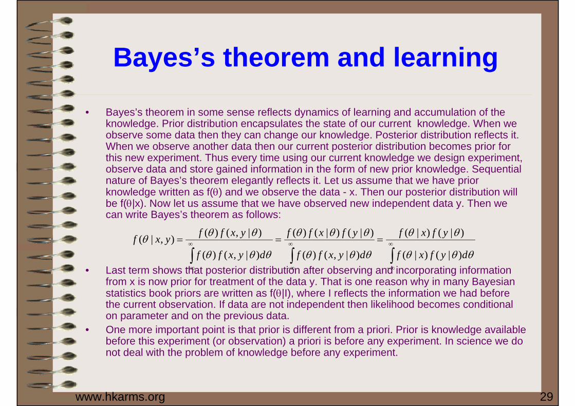
Bayes’s theorem and learning

• Bayes’s theorem in some sense reflects dynamics of learning and accumulation of the knowledge. Prior distribution encapsulates the state of our current knowledge. When we observe some data then they can change our knowledge. Posterior distribution reflects it. When we observe another data then our current posterior distribution becomes prior for this new experiment. Thus every time using our current knowledge we design experiment, observe data and store gained information in the form of new prior knowledge. Sequential nature of Bayes’s theorem elegantly reflects it. Let us assume that we have priorknowledge written as f(θ) and we observe the data - x. Then our posterior distribution will be f(θ|x). Now let us assume that we have observed new independent data y. Then we can write Bayes’s theorem as follows:

• Last term shows that posterior distribution after observing and incorporating information from x is now prior for treatment of the data y. That is one reason why in many Bayesian statistics book priors are written as f(θ|I), where I reflects the information we had before the current observation. If data are not independent then likelihood becomes conditional on parameter and on the previous data.

• One more important point is that prior is different from a priori. Prior is knowledge available before this experiment (or observation) a priori is before any experiment. In science we do not deal with the problem of knowledge before any experiment.

∫∫∫∞

∞−

∞

∞−

∞

∞−

===θθθ

θθ

θθθ

θθθ

θθθ

θθθdyfxf

yfxf

dyxff

yfxff

dyxff

yxffyxf)|()|(

)|()|(

)|,()(

)|()|()(

)|,()(

)|,()(),|(

www.hkarms.org 30

Prior, likelihood and posterior

• Before using Bayes’s theorem as an estimation tool we should have the forms of prior, likelihood and posterior.

• Likelihood is usually derived or approximated using physical properties of the system under study. Usual technique used for derivation of the form of the likelihood is central limit theorem.

• Prior distribution should reflect state of knowledge. Converting knowledge into distribution could be a challenging task. One of the techniques used to derive prior probability distribution is maximum entropy approach. In this approach entropy of distribution is maximised under constraint defined by the available knowledge. Some of the knowledge we have, can easily be incorporated into maximum entropy formalism. Problem with this approach might be that not all available knowledge can easily be used, Another approach is to study the problem, ask experts and build physically sensible prior. One more approach is to find such prior that when used in conjunction with the likelihood they give easy and elegant forms for posterior distributions. These type of priors are called conjugate priors. They depend on the form of likelihood. Here is the list of some of conjugate priors used for one dimensional cases:

• Likelihood Parameter Prior/Posterior• Normal mean (μ) Normal• Normal variance (σ2) Inverse gamma• Poisson λ Beta• Binomial π Gamma

www.hkarms.org 31

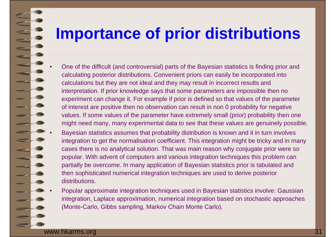
Importance of prior distributions

• One of the difficult (and controversial) parts of the Bayesian statistics is finding prior and calculating posterior distributions. Convenient priors can easily be incorporated into calculations but they are not ideal and they may result in incorrect results and interpretation. If prior knowledge says that some parameters are impossible then no experiment can change it. For example if prior is defined so that values of the parameter of interest are positive then no observation can result in non 0 probability for negative values. If some values of the parameter have extremely small (prior) probability then one might need many, many experimental data to see that these values are genuinely possible.

• Bayesian statistics assumes that probability distribution is known and it in turn involves integration to get the normalisation coefficient. This integration might be tricky and in many cases there is no analytical solution. That was main reason why conjugate prior were so popular. With advent of computers and various integration techniques this problem can partially be overcome. In many application of Bayesian statistics prior is tabulated and then sophisticated numerical integration techniques are used to derive posterior distributions.

• Popular approximate integration techniques used in Bayesian statistics involve: Gaussian integration, Laplace approximation, numerical integration based on stochastic approaches (Monte-Carlo, Gibbs sampling, Markov Chain Monte Carlo).

www.hkarms.org 32