bavirisetty, r., vinayagamoorthy, m., duan, l. …freeit.free.fr/bridge engineering...

Bavirisetty, R., Vinayagamoorthy, M., Duan, L. "Dynamic Analysis." Bridge Engineering Handbook. Ed. Wai-Fah Chen and Lian Duan Boca Raton: CRC Press, 2000

35Dynamic Analysis

35.1 IntroductionStatic vs. Dynamic Analysis • Characteristics of Earthquake Ground Motions • Dynamic Analysis Methods for Seismic Bridge Design

35.2 Single-Degree-of-Freedom SystemEquation of Motion • Characteristics of Free Vibration • Response to Earthquake Ground Motion • Response Spectra • Example of an SDOF system

35.3 Multi-Degree-of-Freedom SystemEquation of Motion • Free Vibration and Vibration Modes • Modal Analysis and Modal Participation factor • Example of an MDOF system • Multiple-Support Excitation • Time History Analysis

35.4 Response Spectrum AnalysisSingle-Mode Spectral Analysis • Uniform-Load Method • Multimode Spectral Analysis • Multiple-Support Response Spectrum Method

35.5 Inelastic Dynamic AnalysisEquations of Motion • Modeling Considerations

35.6 Summary

35.1 Introduction

The primary purpose of this chapter is to present dynamic methods for analyzing bridge structureswhen subjected to earthquake loads. Basic concepts and assumptions used in typical dynamicanalysis are presented first. Various approaches to bridge dynamics are then discussed. A fewexamples are presented to illustrate their practical applications.

35.1.1 Static vs. Dynamic Analysis

The main objectives of a structural analysis are to evaluate structural behavior under various loadsand to provide the information necessary for design, such as forces, moments, and deformations.Structural analysis can be classified as static or dynamic: while statics deals with time-independentloading, dynamics considers any load where the magnitude, direction, and position vary with time.Typical dynamic loads for a bridge structure include vehicular motions and wave actions such aswinds, stream flow, and earthquakes.

Rambabu BavirisettyCalifornia Department

of Transportation

Murugesu VinayagamoorthyCalifornia Department

of Transportation

Lian DuanCalifornia Department

of Transportation

© 2000 by CRC Press LLC

35.1.2 Characteristics of Earthquake Ground Motions

An earthquake is a natural ground movement caused by various phenomena including globaltectonic processes, volcanism, landslides, rock-bursts, and explosions. The global tectonic processesare continually producing mountain ranges and ocean trenches at the Earth’s surface and causingearthquakes. This section briefly discusses the earthquake input for seismic bridge analysis. Detaileddiscussions of ground motions are presented in Chapter 33.

Ground motion is represented by the time history or seismograph in terms of acceleration,velocity, and displacement for a specific location during an earthquake. Time history plots containcomplete information about the earthquake motions in the three orthogonal directions (two hor-izontal and one vertical) at the strong-motion instrument location. Acceleration is usually recordedby strong-motion accelerograph and the velocities and displacements are determined by numericalintegration. The accelerations recorded at locations that are approximately the same distance awayfrom the epicenter may differ significantly in duration, frequency content, and amplitude due todifferent local soil conditions. Figure 35.1 shows several time histories of recent earthquakes.

From a structural engineering view, the most important characteristics of an earthquake are thepeak ground acceleration (PGA), duration, and frequency content. The PGA is the maximumacceleration and represents the intensity of a ground motion. Although the ground velocity maybe a more significant measure of intensity than the acceleration, it is not often measured directly,but determined using supplementary calculations [1]. The duration is the length of time betweenthe first and the last peak exceeding a specified strong motion level. The longer the duration of astrong motion, the more energy is imparted to a structure. Since the elastic strain energy absorbedby a structure is very limited, a longer strong earthquake has a greater possibility to enforce astructure into the inelastic range. The frequency content can be represented by the number of zerocrossings per second in the accelerogram. It is well understood that when the frequency of a regulardisturbing force is the same as the natural vibration frequency of a structure (resonance), theoscillation of structure can be greatly magnified and effects of damping become minimal. Although

FIGURE 35.1 Ground motions recorded during recent earthquakes.


earthquake motions are never as regular as a sinusoidal waveform, there is usually a period thatdominates the response.

Since it is impossible to measure detailed ground motions for all structure sites, the rock motionsor ground motions are estimated at a fault and then propagated to the Earth surface using a computerprogram considering the local soil conditions. Two guidelines [2, 3] recently developed by theCalifornia Department of Transportation provide the methods to develop seismic ground motionsfor bridges.

35.1.3 Dynamic Analysis Methods for Seismic Bridge Design

Depending on the seismic zone, geometry, and importance of the bridge, the following analysismethods may be used for seismic bridge design:

• The single-mode method (single-mode spectral and uniform load analysis) [4,5] assumesthat seismic load can be considered as an equivalent static horizontal force applied to anindividual frame in either the longitudinal or transverse direction. The equivalent static forceis based on the natural period of a single degree of freedom (SDOF) and code-specifiedresponse spectra. Engineers should recognize that the single-mode method (sometimesreferred to as equivalent static analysis) is best suited for structures with well-balanced spanswith equally distributed stiffness.

• Multimode spectral analysis assumes that member forces, moments, and displacements dueto seismic load can be estimated by combining the responses of individual modes using themethods such as complete quadratic combination (CQC) method and the square root of thesum of the squares (SRSS) method. The CQC method is adequate for most bridge systems[6], and the SRSS method is best suited for combining responses of well-separated modes.

• The multiple support response spectrum (MSRS) method provides response spectra and thepeak displacements at individual support degrees of freedom by accurately accounting forthe spatial variability of ground motions including the effects of incoherence, wave passage,and spatially varying site response. This method can be used for multiply supported longstructures [7].

• The time history method is a numerical step-by-step integration of equations of motion. Itis usually required for critical/important or geometrically complex bridges. Inelastic analysisprovides a more realistic measure of structural behavior when compared with an elasticanalysis.

Selection of the analysis method for a specific bridge structure should not be purely based onperforming structural analysis, but be based on the effective design decisions [8]. Detailed discus-sions of the above methods are presented in the following sections.

35.2 Single-Degree-of-Freedom System

The familiar spring–mass system represents the simplest dynamic model and is shown inFigure 35.2a. When the idealized, undamped structures are excited by either moving the support orby displacing the mass in one direction, the mass oscillates about the equilibrium state foreverwithout coming to rest. But, real structures do come to rest after a period of time due to aphenomenon called damping. To incorporate the effect of the damping, a massless viscous damperis always included in the dynamic model, as shown in Figure 35.2b.

In a dynamic analysis, the number of displacements required to define the displaced positionsof all the masses relative to their original positions is called the number of degrees of freedom(DOF). When a structural system can be idealized with a single mass concentrated at one locationand moved only in one direction, this dynamic system is called an SDOF system. Some structures,


such as a water tank supported by a single-column, one-story frame structure and a two-span bridgesupported by a single column, could be idealized as SDOF models (Figure 35.3).

In the SDOF system shown in Figure 35.3c, the mass of the bridge superstructure is the mass ofthe dynamic system. The stiffness of the dynamic system is the stiffness of the column against sidesway and the viscous damper of the system is the internal energy absorption of the bridge structure.

35.2.1 Equation of Motion

The response of a structure depends on its mass, stiffness, damping, and applied load or displace-ment. The structure could be excited by applying an external force p(t) on its mass or by a ground

FIGURE 35.2 Idealized dynamic model. (a) Undamped SDOF system; (b) damped SDOF system.

FIGURE 35.3 Examples of SDOF structures. (a) Water tank supported by single column; (b) one-story framebuilding; (c) two-span bridge supported by single column.


motion u(t) at its supports. In this chapter, since the seismic loading is induced by exciting thesupport, we focus mainly on the equations of motion of an SDOF system subjected to groundexcitation.

The displacement of the ground motion , the total displacement of the single mass , andthe relative displacement between the mass and ground u (Figure 35.4) are related by

(35.1)

By applying Newton’s law and D’Alembert’s principle of dynamic equilibrium, it can be shownthat

(35.2)

where is the inertial force of the single mass and is related to the acceleration of the mass by; is the damping force on the mass and related to the velocity across the viscous damper

by ; is the elastic force exerted on the mass and related to the relative displacementbetween the mass and the ground by , where k is the spring constant; c is the dampingratio; and m is the mass of the dynamic system.

Substituting these expressions for , , and into Eq. (35.2) gives

(35.3)

The equation of motion for an SDOF system subjected to a ground motion can then be obtainedby substituting the Eq. (35.1) into Eq. (35.3), and is given by

(35.4)

35.2.2 Characteristics of Free Vibration

To determine the characteristics of the oscillations such as the time to complete one cycle ofoscillation ( ) and number of oscillation cycles per second ( ), we first look at the free vibrationof a dynamic system. Free vibration is typically initiated by disturbing the structure from its

FIGURE 35.4 Earthquake–induced motion of an SDOF system.

ug ut

u u ut g= +

f f fI D S+ + =0

fI

f muI t= ˙̇ fD

f cuD = ˙ fS

f k uS =

fI fD fS

mu cu k ut˙̇ ˙+ + =0

mu cu k u mug˙̇ ˙ ˙̇+ + = −

Tn ωn


equilibrium state by an external force or displacement. Once the system is disturbed, the systemvibrates without any external input. Thus, the equation of motion for free vibration can be obtainedby setting to zero in Eq. (35.4) and is given by

(35.5)

Dividing the Equation (35.5) by its mass m will result in

(35.6)

(35.7)

where the natural circular frequency of vibration or the undamped frequency; the damping ratio; the critical damping coefficient.

Figure 35.5a shows the response of a typical idealized, undamped SDOF system. The time requiredfor the SDOF system to complete one cycle of vibration is called the natural period of vibration( ) of the system and is given by

FIGURE 35.5 Typical response of an SDOF system. (a) Undamped; (b) damped.

˙̇ug

mu cu k u˙̇ ˙+ + =0

˙̇ ˙ucm

ukm

u+ +

= 0

˙̇u un n+ + =2 02ξω ω

ωn k m= /ξ = c ccr c m k m kcr n n= = =2 2 2ω ω

Tn


(35.8)

Furthermore, the natural cyclic frequency of vibration is given by

(35.9)

Figure 35.5b shows the response of a typical damped SDOF structure. The circular frequency ofthe vibration or damped vibration frequency of the SDOF structure, , is given by

.The damped period of vibration ( ) of the system is given by

(35.10)

When or the structure returns to its equilibrium position without oscillating andis referred to as a critically damped structure. When or , the structure is overdampedand comes to rest without oscillating, but at a slower rate. When or , the structure isunderdamped and oscillates about its equilibrium state with progressively decreasing amplitude.Figure 35.6 shows the response of SDOF structures with different damping ratios.

For structures such as buildings, bridges, dams, and offshore structures, the damping ratio is lessthan 0.15 and thus can be categorized as underdamped structures. The basic dynamic propertiesestimated using damped or undamped assumptions are approximately the same. For example, when

, , and Damping dissipates the energy out of a structure in opening and closing of microcracks in

concrete, stressing of nonstructural elements, and friction at the connection of steel members. Thus,the damping coefficient accounts for all energy-dissipating mechanisms of the structure and canonly be estimated by experimental methods. Two seemingly identical structures may have slightlydifferent material properties and may dissipate energy at different rates. Since damping does not

FIGURE 35.6 Response of an SDOF system for various damping ratios.

Tmkn

n

= =22

πω

π

fn

f nωn

2π------

12π------ k

m----= =

ωd

ω ω ξd n= −1 2

Td

Tmkd

d

= =−

2 2

1 2

πω

πξ

ξ = 1 c ccr=ξ >1 c ccr>

ξ < 1 c ccr<

ξ = 0 10. ω ωd n= 0 995. T Td n=1 01. .


play an important quantitative role except for resonant responses in structural responses, it iscommon to use average damping ratios based on the types of construction materials. Relativedamping ratios for common types of structures, such as welded metal of 2 to 4%, bolted metalstructures of 4 to 7%, prestressed concrete structures of 2 to 5%, reinforced-concrete structures of4 to 7% and wooden structures of 5 to 10%, are recommended by Chmielewski et al. [9].

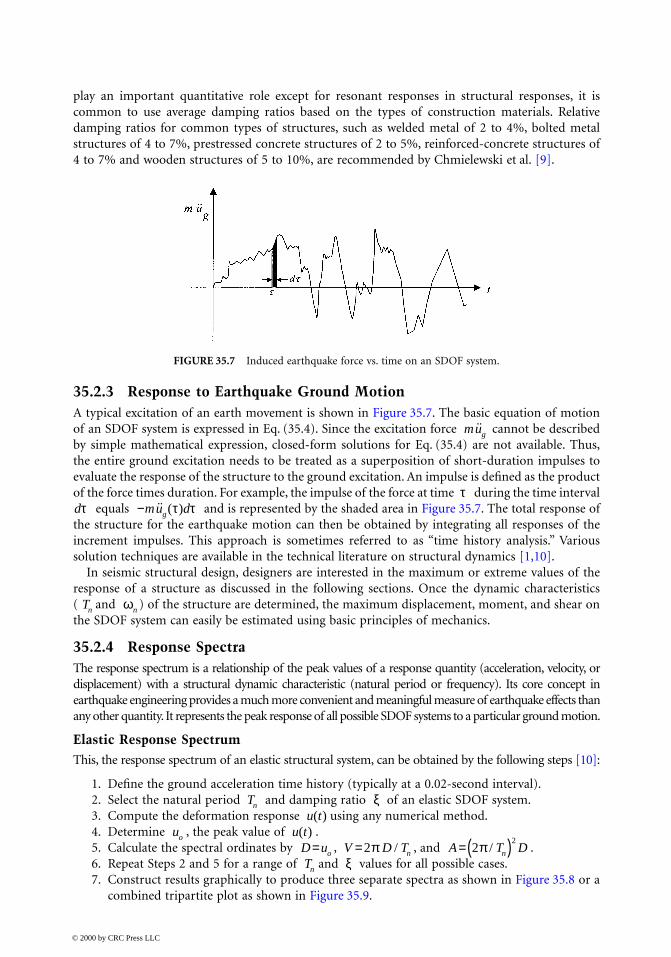
35.2.3 Response to Earthquake Ground MotionA typical excitation of an earth movement is shown in Figure 35.7. The basic equation of motionof an SDOF system is expressed in Eq. (35.4). Since the excitation force cannot be describedby simple mathematical expression, closed-form solutions for Eq. (35.4) are not available. Thus,the entire ground excitation needs to be treated as a superposition of short-duration impulses toevaluate the response of the structure to the ground excitation. An impulse is defined as the productof the force times duration. For example, the impulse of the force at time during the time interval

equals and is represented by the shaded area in Figure 35.7. The total response ofthe structure for the earthquake motion can then be obtained by integrating all responses of theincrement impulses. This approach is sometimes referred to as “time history analysis.” Varioussolution techniques are available in the technical literature on structural dynamics [1,10].

In seismic structural design, designers are interested in the maximum or extreme values of theresponse of a structure as discussed in the following sections. Once the dynamic characteristics( and ) of the structure are determined, the maximum displacement, moment, and shear onthe SDOF system can easily be estimated using basic principles of mechanics.

35.2.4 Response SpectraThe response spectrum is a relationship of the peak values of a response quantity (acceleration, velocity, ordisplacement) with a structural dynamic characteristic (natural period or frequency). Its core concept inearthquake engineering provides a much more convenient and meaningful measure of earthquake effects thanany other quantity. It represents the peak response of all possible SDOF systems to a particular ground motion.

Elastic Response SpectrumThis, the response spectrum of an elastic structural system, can be obtained by the following steps [10]:

1. Define the ground acceleration time history (typically at a 0.02-second interval).2. Select the natural period and damping ratio of an elastic SDOF system.3. Compute the deformation response using any numerical method.4. Determine , the peak value of .5. Calculate the spectral ordinates by , , and .6. Repeat Steps 2 and 5 for a range of and values for all possible cases.7. Construct results graphically to produce three separate spectra as shown in Figure 35.8 or a

combined tripartite plot as shown in Figure 35.9.

FIGURE 35.7 Induced earthquake force vs. time on an SDOF system.

mug˙̇

τdτ −mu dg

˙̇ ( )τ τ

Tn ωn

Tn ξu t( )

uo u t( )D uo= V D Tn=2π / A T Dn=( )2

2π/

Tn ξ



It is noted that although three spectra (displacement, velocity, and acceleration) for a specificground motion contain the same information, each provides a physically meaningful quantity. Thedisplacement spectrum presents the peak displacement. The velocity spectrum is related directly tothe peak strain energy stored in the system. The acceleration spectrum is related directly to the peakvalue of the equivalent static force and base shear.

A response spectrum (Figure 35.9) can be divided into three ranges of periods [10]:

• Acceleration-sensitive region (very short period region): A structure with a very short periodis extremely stiff and expected to deform very little. Its mass moves rigidly with the groundand its peak acceleration approximately equals the ground acceleration.

• Velocity-sensitive region (intermediate-period region): A structure with an intermediateperiod responds greatly to the ground velocity than other ground motion parameters.

• Displacement-sensitive region (very long period region): A structure with a very long period is extremelyflexible and expected to remain stationary while the ground moves. Its peak deformation is closer tothe ground displacement. The structural response is most directly related to ground displacement.

Elastic Design SpectrumSince seismic bridge design is intended to resist future earthquakes, use of a response spectrum obtainedfrom a particular past earthquake motion is inappropriate. In addition, jagged spectrum values oversmall ranges would require an unreasonable accuracy in the determination of the structure period [11].It is also impossible to predict a jagged response spectrum in all its details for a ground motion thatmay occur in the future. To overcome these shortcomings, the elastic design spectrum, a smoothenedidealized response spectrum, is usually developed to represent the envelopes of ground motions recordedat the site during past earthquakes. The development of an elastic design spectrum is based on statisticalanalysis of the response spectra for the ensemble of ground motions. Figure 35.10 shows a set of elasticdesign spectra in Caltrans Bridge Design Specifications [12]. Figure 35.11 shows project-specific accel-eration response spectra for the California Sonoma Creek Bridge.

FIGURE 35.8 Example of response spectra (5% critical damping) for Loma Prieta 1989 motion.

Engineers should recognize the conceptual differences between a response spectrum and a designspectrum [10]. A response spectrum is only the peak response of all possible SDOF systems due toa particular ground motion, whereas a design spectrum is a specified level of seismic design forcesor deformations and is the envelope of two different elastic design spectra. The elastic designspectrum provides a basis for determining the design force and deformation for elastic SDOFsystems.

Inelastic Response SpectrumA bridge structure may experience inelastic behavior during a major earthquake. The typical elasticand elastic–plastic responses of an idealized SDOF to severe earthquake motions are shown inFigure 35.12. The input seismic energy received by a bridge structure is dissipated by both viscousdamping and yielding (localized inelastic deformation converting into heat and other irrecoverableforms of energy). Both viscous damping and yielding reduce the response of inelastic structurescompared with elastic structures. Viscous damping represents the internal friction loss of a structurewhen deformed and is approximately a constant because it depends mainly on structural materials.Yielding, on the other hand, varies depending on structural materials, structural configurations,and loading patterns and histories. Damping has negligible effects on the response of structures for

FIGURE 35.9 Tripartite plot–response spectra (1994 Northridge Earthquake, Arleta–Rordhoff Ave. Fire Station).


the long-period and short-period systems and is most effective in reducing response of structuresfor intermediate-period systems.

In seismic bridge design, a main objective is to ensure that a structure is capable of deformingin a ductile manner when subjected to a larger earthquake loading. It is desirable to consider theinelastic response of a bridge system to a major earthquake. Although a nonlinear inelastic dynamicanalysis is not difficult in concept, it requires careful structural modeling and intensive computing

FIGURE 35.10 Typical Caltrans elastic design response spectra.

FIGURE 35.11 Acceleration response spectra for Sonoma Creek Bridge.


effort [8]. To consider inelastic seismic behavior of a structure without performing a true nonlinearinelastic analysis, the ductility-factor method can be used to obtain the inelastic response spectrafrom the elastic response spectra. The ductility of a structure is usually referred as the displacementductility factor defined by (Figure 35.13):

(35.11)

where ∆u is ultimate displacement capacity and is yield displacement.The simplest approach to developing the inelastic design spectrum is to scale the elastic design

spectrum down by some function of the available ductility of a structural system:

(35.12)

(35.13)

FIGURE 35.12 Response of an SDOF to earthquake ground motions. (a) Elastic system; (b) inelastic system.

µ

µ =∆∆

u

y

∆ y

ARSARS

finelasticelastic= ( )µ

f µ( )

1

2µ 1–

µ

=

for T n 0.03 sec.≤

for 0.03 sec. T n 0.5 sec.≤<

for T n 0.5 sec.≥


For very short period ( ≤ 0.03 sec) in the acceleration-sensitive region, the elastic displacementdemand is less than displacement capacity (see Figure 35.13). The reduction factor

implies that the structure should be designed and remained at elastic to avoid excessiveinelastic deformation. For intermediate period (0.03 sec < ≤ 0.5 sec) in the velocity-sensitive region,elastic displacement demand may be greater or less than displacement capacity and thereduction factor is based on the equal-energy concept. For the very long period ( > 0.5 sec) in thedisplacement-sensitive region, the reduction factor is based on the equal displacement concept.

35.2.5 Example of an SDOF system

GivenAn SDOF bridge structure is shown in Figure 35.14. To simplify the problem, the bridge is assumedto move only in the longitudinal direction. The total resistance against the longitudinal motioncomes in the form of friction at bearings and this could be considered a damper. Assume thefollowing properties for the structure: damping ratio ξ = 0.05, area of superstructure A = 3.57 m2,moment of column Ic = 0.1036 m4, Ec of column = 20,700 MPa, material density ρ = 2400 kg/m3,length of column Lc = 9.14 m, and length of the superstructure Ls = 36.6 m. The acceleration responsecurve of the structure is given in the Figure 35.11. Determine (1) natural period of the structure,(2) damped period of the structure, (3) maximum displacement of the superstructure, and (4)maximum moment in the column.

Solution

Stiffness: N/m

Mass: kg

Natural circular frequency: rad/s

FIGURE 35.13 Lateral load–displacement relations.

Tn

∆ed ∆u

f µ( ) = 1Tn

∆ed ∆u

Tn

kE I

Lc c

c

= = × =12 12 20700 10 0 1036

9 14336903013

6

3

( )( . ).

m A Ls= = =ρ ( . )( . )( ) , .3 57 36 6 2400 313 588 8

ωn

km

= = =33 690 301313 588 8

10 36, ,

, ..


Natural cyclic frequency: cycles/s

Natural period of the structure: s

The damped circular frequency is given by

rad/s

The damped period of the structure is given by

s

From the ARS curve, for a period of 0.606 s, the maximum acceleration of the structure will be0.9 g = 1.13 × 9.82 = 11.10 m/s. Then,

The force acting on the mass =

The maximum displacement

The maximum moment in the column

FIGURE 35.14 SDOF bridge example. (a) Two-span bridge schematic diagram; (b) single column bent; (c) idealizedequivalent model for longitudinal response.

fnn= = =ωπ π2

10 362

1 65.

.

Tfnn

= = =1 11 65

0 606.

.

ω ω ξd n= − = − =1 10 36 1 0 05 10 332 2. . .

Tdd

= = =2 210 33

0 608π

ωπ.

.

m × = × =11 10 313588 8 11 10 3 48. . . . MN

= = ×× ×

=FLEI

c

c

3 3

123 48 9 14

12 20700 0 10360 103

. ..

. m

= = × =FLc

23 48 9 14

215 90

. .. MN-m


35.3 Multidegree-of-Freedom System

The SDOF approach may not be applicable for complex structures such as multilevel frame structureand bridges with several supports. To predict the response of a complex structure, the structure isdiscretized with several members of lumped masses. As the number of lumped masses increases,the number of displacements required to define the displaced positions of all masses increases. Theresponse of a multidegree of freedom (MDOF) system is discussed in this section.

35.3.1 Equation of Motion

The equation of motion of an MDOF system is similar to the SDOF system, but the stiffness k,mass m, and damping c are matrices. The equation of motion to an MDOF system under groundmotion can be written as

(35.14)

The stiffness matrix can be obtained from standard static displacement-based analysismodels and may have off-diagonal terms. The mass matrix due to the negligible effect of masscoupling can best be expressed in the form of tributary lumped masses to the correspondingdisplacement degree of freedoms, resulting in a diagonal or uncoupled mass matrix. The dampingmatrix accounts for all the energy-dissipating mechanisms in the structure and may have off-diagonal terms. The vector is a displacement transformation vector that has values 0 and 1to define degrees of freedoms to which the earthquake loads are applied.

35.3.2 Free Vibration and Vibration Modes

To understand the response of MDOF systems better, we look at the undamped, free vibration ofan N degrees of freedom (N-DOF) system first.

Undamped Free VibrationBy setting and to zero in the Eq. (35.14), the equation of motion of undamped, freevibration of an N-DOF system can be shown as:

(35.15)

where and are n × n square matrices.

Equation (35.15) could then be rearranged to

(35.16)

where is the deflected shape matrix. Solution to this equation can be obtained by setting

(35.17)

The roots or eigenvalues of Eq. (35.17) will be the N natural frequencies of the dynamic system.Once the natural frequencies ( ) are estimated, Eq. (35.16) can be solved for the correspondingN independent, deflected shape matrices (or eigenvectors), . In other words, a vibrating system

M C K M B[ ]{ } + [ ] { } + [ ] { } = −[ ] { }˙̇ ˙ ˙̇u u u ug

K[ ]M[ ]

C[ ]B{ }

C[ ] ˙̇ug

M K[ ] { } + [ ] { } =˙̇u u 0

M[ ] K[ ]

[ ] [ ] { }K M−

=ω φn n2 0

φn{ }

K M[ ] − [ ] =ωn2 0

ωn

φn{ }


with N-DOFs will have N natural frequencies (usually arranged in sequence from smallest to largest),corresponding N natural periods Tn, and N natural mode shapes . These eigenvectors aresometimes referred to as natural modes of vibration or natural mode shapes of vibration. It isimportant to recognize that the eigenvectors or mode shapes represent only the deflected shapecorresponding to the natural frequency, not the actual deflection magnitude.

The N eigenvectors can be assembled in a single n × n square matrix , modal matrix, whereeach column represents the coefficients associated with the natural mode. One of the importantaspects of these mode shapes is that they are orthogonal to each other. Stated mathematically,

If , and (35.18)

(35.19)

(35.20)

where and have off-diagonal elements, whereas and are diagonal matrices.

Damped Free VibrationWhen damping of the MDOF system is included, the free vibration response of the damped systemwill be given by

(35.21)

The displacements are first expressed in terms of natural mode shapes, and later they are multi-plied by the transformed natural mode matrix to obtain the following expression:

(35.22)

where, and are diagonal matrices given by Eqs. (35.19) and (35.20) and

(35.23)

While and are diagonal matrices, may have off diagonal terms. When hasoff diagonal terms, the damping matrix is referred to as a nonclassical or nonproportional dampingmatrix. When is diagonal, it is referred to as a classical or proportional damping matrix.Classical damping is an appropriate idealization when similar damping mechanisms are distributedthroughout the structure. Nonclassical damping idealization is appropriate for the analysis whenthe damping mechanisms differ considerably within a structural system.

Since most bridge structures have predominantly one type of construction material, bridgestructures could be idealized as a classical damping structural system. Thus, the damping matrixof Eq. (35.22) will be a diagonal matrix for most bridge structures. And, the equation of nth modeshape or generalized nth modal equation is given by

(35.24)

Equation (35.24) is similar to the Eq. (35.7) of an SDOF system. Also, the vibration propertiesof each mode can be determined by solving the Eq. (35.24).

φn{ }

ΦΦ[ ]

ω ωn r≠ φ φn

T

rK{ } [ ] { } = 0 φ φn

T

rM{ } [ ] { } = 0

K KT*[ ] =[ ] [ ] [ ]Φ Φ

M MT*[ ] =[ ] [ ] [ ]Φ Φ

K[ ] M[ ] K*[ ] M*[ ]

M C K[ ]{ } + [ ]{ } + [ ]{ } =˙̇ ˙u u u 0

M C K* * *˙̇ ˙[ ] { } + [ ]{ } + [ ] { } =Y Y Y 0

M*[ ] K*[ ]C C*[ ] =[ ] [ ] [ ]ΦΦ ΦΦT

M*[ ] K*[ ] C*[ ] C*[ ]C*[ ]

˙̇ ˙Y Y Yn n n n n+ + =2 02ξ ω ω


Rayleigh DampingThe damping of a structure is related to the amount of energy dissipated during its motion. It couldbe assumed that a portion of the energy is lost due to the deformations, and thus damping couldbe idealized as proportional to the stiffness of the structure. Another mechanism of energy dissi-pation could be attributed to the mass of the structure, and thus damping idealized as proportionalto the mass of the structure. In Rayleigh damping, it is assumed that the damping is proportionalto the mass and stiffness of the structure.

(35.25)

The generalized damping of the nth mode is then given by

(35.26)

(35.27)

(35.28)

(35.29)

Figure 35.15 shows the Rayleigh damping variation with natural frequency. The coefficientsand can be determined from specified damping ratios at two independent dominant modes

(say, ith and jth modes). Expressing Eq. (35.29) for these two modes will lead to the followingequations:

(35.30)

(35.31)

FIGURE 35.15 Rayleigh damping variation with natural frequency.

C M K[ ] = [ ] + [ ]a ao 1

C a M a Kn o n n= + 1

C a M a Mn o n n n= + 12ω

ξωnn

n n

C

M=

2

ξω

ωno

nn

a a= +2

1

21

ao a1

ξω

ωio

ii

a a= +2

1

21

ξω

ωjo

jj

a a= +2

1

21


When the damping ratio at both the ith and jth modes is the same and equals , it can be shownthat

(35.32)

It is important to note that the damping ratio at a mode between the ith and jth mode is less than. And, in practical problems the specified damping ratios should be chosen to ensure reasonable

values in all the mode shapes that lie between the ith and jth mode shapes.

35.3.3 Modal Analysis and Modal Participation Factor

In previous sections, we have discussed the basic vibration properties of an MDOF system. Now,we will look at the response of an MDOF system to earthquake ground motion. The basic equationof motion of the MDOF for an earthquake ground motion given by Eq. (35.14) is repeated here:

The displacement is first expressed in terms of natural mode shapes, and later it is multiplied bythe transformed natural mode matrix to obtain the following expression:

(35.33)

And, the equation of the nth mode shape is given by

(35.34)

where (35.35)

(35.36)

The Ln is referred to as the modal participation factor of the nth mode.By dividing the Eq. (35.34) by , the generalized modal equation of the nth mode becomes

(35.37)

Equation (35.34) is similar to the equation motion of an SDOF system, and thus can bedetermined by using methods similar to those described for SDOF systems. Once is established,the displacement due to the nth mode will be given by . The total displacement dueto combination of all mode shapes can then be determined by summing up all displacements foreach mode and is given by

(35.38)

ξ

aoi j

i j

=+

ξω ω

ω ω2

ai j

1

2=+

ξω ω

ξ

M C K M[ ]{ } + [ ]{ } + [ ]{ } = −[ ] { }˙̇ ˙ ˙̇u u u B ug

M C K M* * *˙̇ ˙ ˙̇[ ] { } + [ ]{ } + [ ] { } = −[ ] [ ] { }Y Y Y B uTgΦΦ

M Y M Y M Y L un n n n n n n n n g* * *˙̇ ˙ ˙̇+ + =2 2ξ ω ω

Mn n

T

n* = { } [ ] { }φ φM

Ln n

T= −{ } [ ] [ ]φ M B

Mn*

˙̇ ˙ ˙̇*Y Y Y

L

Mun n n n n

n

ng+ + =

2 2ξ ω ω

Yn

Yn

u t Y tn n n( ) ( )=φ

u t Y tn n( ) ( )=∑φ


This approach is sometimes referred to as the classical mode superposition method. Similar tothe estimation of the total displacement, the element forces can also be estimated by adding theelement forces for each mode shape.

35.3.4 Example of an MDOF System

GivenThe bridge shown in Figure 35.16 is a three-span continuous frame structure. Details of the bridgeare as follows: span lengths are 18.3, 24.5, and 18.3 m.; column length is 9.5 m; area of superstructureis 5.58 m2; moment of inertia of superstructure is 70.77 m4; moment of inertia of column is 0.218m4; modulus of elasticity of concrete is 20,700 MPa. Determine the vibration modes and frequenciesof the bridge.

SolutionAs shown in Figures 35.16b, c, and d, five degrees of freedom are available for this structure. Stiffnessand mass matrices are estimated separately and the results are given here.

FIGURE 35.16 Three-span continuous framed bridge structure of MDOF example. (a) Schematic diagram; (b)longitudinal degree of freedom; (c) transverse degree of freedom; (d) rotational degree of freedom; (e) mode shape 1;(f) mode shape 2; (g) mode shape 3.


Condensation procedure will eliminate the rotational degrees of freedom and will result in threedegrees of freedom. (The condensation procedure is performed separately and the result is givenhere.) The equation of motion of free vibration of the structure is

Substituting condensed stiffness and mass matrices into the above equation gives

The above equation can be rearranged in the following form:

Substitution of appropriate values in the above expression gives the following

By assuming different vibration modes, natural frequencies of the structure can be estimated.

K[ ] =− − −

−

−

−

126318588 0 0 0 0

0 1975642681 1194370500 1520122814 14643288630

0 1194370500 1975642681 14643288630 1520122814

0 1520122814 14643288630 479327648712 119586857143

0 14643288630 1520122814 119586857143 479327648712

M[ ] =

81872 0 0 0 0

0 286827 0 0 0

0 0 286827 0 0

0 0 0 0 0

0 0 0 0 0

M u K u[ ]{ } + [ ]{ } = { }˙̇ 0

81872 0 0

0 286827 0

0 0 286827

126318588 0 0

0 1975642681 1194370500

0 1194370500 1975642681

0

0

0

1

2

3

1

2

3

+ −

−

=

˙̇

˙̇

˙̇

u

u

u

u

u

u

12

1

ωφ φM K[ ] [ ] { } = { }−

1

1818172

0 0

01

2868270

0 01

286827

126318588 0 0

0 1518171572 1215625977

0 1215625977 15181715722

1

2

3

1

2

3

ω

φφφ

φφφn

n

n

n

n

n

n

−−

=

1154 39 0 0

0 5292 9 4238 2

0 4238 2 5292 92

1

2

3

1

2

3

ω

φφφ

φφφn

n

n

n

n

n

n

.

. .

. .

−−

=


Substitution of vibration mode will result in the first natural frequency.

Thus, By substituting the vibration modes of and in the above expression, the

other two natural frequencies are estimated as 32.48 and 97.63 rad/s.

35.3.5 Multiple-Support Excitation

So far we have assumed that all supports of a structural system undergo the same ground motion.This assumption is valid for structures with foundation supports close to each other. However, forlong-span bridge structures, supports may be widely spaced. As described in Section 35.1.2, earthmotion at a location depends on the localized soil layer and the distance from the epicenter. Thus,bridge structures with supports that lie far from each other may experience different earth excitation.For example, Figure 35.17c, d, and e shows the predicted earthquake motions at Pier W3 andPier W6 of the San Francisco–Oakland Bay Bridge (SFOBB) in California. The distance betweenPier W3 and Pier W6 of the SFOBB is approximately 1411 m. These excitations are predicted bythe California Department of Transportation by considering the soil and rock properties in thevicinity of the SFOBB and expected Earth movements at the San Andreas and Hayward faults. Notethat the Earth motion at Pier W3 and Pier W6 are very different. Furthermore, Figures 35.17c, d,and e indicates that the Earth motion not only varies with the location, but also varies with direction.Thus, to evaluate the response of long, multiply supported, and complicated bridge structures, useof the actual earthquake excitation at each support is recommended.

The equation of motion of a multisupport excitation would be similar to Eq. (35.14), but theonly difference is now that is replaced by an displacement array . And, the equationof motion for the multisupport system becomes

(35.39)

where has the acceleration at each support locations and has zero value at nonsupportlocations. By using the uncoupling procedure described in the previous sections, the modal equationof the nth mode can be written as

(35.40)

where Ng is the total number of externally excited supports.The deformation response of the nth mode can then be determined as described in previous

sections. Once the displacement responses of the structure for all the mode shapes are estimated,the total dynamic response can be obtained by combining the displacements.

35.3.6 Time History Analysis

When the structure enters the nonlinear range, or has nonclassical damping properties, modalanalysis cannot be used. A numerical integration method, sometimes referred to as time historyanalysis, is required to get more accurate responses of the structure.

1 0 0{ } T

1154 39 0 0

0 5292 9 4238 2

0 4238 2 5292 9

1

0

0

1154 39

0

0

1

0

02 2ω ωn n

.

. .

. .

.

−−

=

=

ω ωn n2 154 39 12 43= =. .and rad / s

0 1 1{ } T0 1 1–{ } T

B ug{ } ˙̇ ˙̇ug{ }

M C K M[ ] { } + [ ] { } + [ ] { } = −[ ] { }˙̇ ˙ ˙̇u u u ug

˙̇ug{ }

˙̇ ˙ ˙̇*Y Y Y

L

Mun n n n n

n

ng

l

Ng

+ + = −=∑2 2

1

ξ ω ω


In a time history analysis, the timescale is divided into a series of smaller steps, dτ. Let us say theresponse at ith time interval has already determined and is denoted by . Then, the responseof the system at ith time interval will satisfy the equation of motion (Eq. 35.39).

(35.41)

FIGURE 35.17 San Francisco–Oakland Bay Bridge. (a) Vicinity map; (b) general plan elevation; (c) longitudinalmotion at rock level; (d) transverse motion at rock level; (e) vertical motion at rock level; (f) displacement responseat top of Pier W3.

u u ui i i, ˙ , ˙̇

M C K M[ ] { } + [ ]{ } + [ ]{ } = −[ ] { }˙̇ ˙ ˙̇u u u ui i i gi


The time-stepping method enables us to step ahead and determine the responses atthe i + 1th time interval by satisfying Eq. (35.39). Thus, the equation of motion at i + 1th time intervalwill be

(35.42)

Equation (35.42) needs to be solved prior to proceeding to the next time step. By stepping throughall the time steps, the actual response of the structure can be determined at all time instants.

Example of Time History AnalysisThe Pier W3 of the SFOBB was modeled using the ADINA [13] program and nonlinear analysiswas performed using the displacement time histories. The displacement time histories in threedirections are applied at the bottom of the Pier W3 and the response of the Pier W3 was studiedto estimate the demand on Pier W3. One of the results, the displacement response at top of Pier W3,is shown in Figure 35.17f.

35.4 Response Spectrum Analysis

Response spectrum analysis is an approximate method of dynamic analysis that gives the maximumresponse (acceleration, velocity, or displacement) of an SDOF system with the same damping ratio,but with different natural frequencies, respond to a specified seismic excitation. Structural modelswith n degrees of freedom can be transformed to n single-degree systems and response spectraprinciples can be applied to systems with many degrees of freedom. For most ordinary bridges, acomplete time history is not required. Because the design is generally based on the maximumearthquake response, response spectrum analysis is probably the most common method used indesign offices to determine the maximum structural response due to transient loading. In thissection, we will discuss basic procedures of response spectrum analysis for bridge structures.

35.4.1 Single-Mode Spectral Analysis

Single-mode spectral analysis is based on the assumption that earthquake design forces for structuresrespond predominantly in the first mode of vibration. This method is most suitable to regular linearelastic bridges to compute the forces and deformations, but is not applicable to irregular bridges(unbalanced spans, unequal stiffness in the columns, etc.) because higher modes of vibration affectthe distribution of the forces and resulting displacements significantly. This method can be appliedto both continuous and noncontinuous bridge superstructures in either the longitudinal or trans-verse direction. Foundation flexibility at the abutments can be included in the analysis.

Single-mode analysis is based on Rayleigh’s energy method — an approximate method whichassumes a vibration shape for a structure. The natural period of the structure is then calculated byequating the maximum potential and kinetic energies associated with the assumed shape. Theinertial forces are calculated using the natural period, and the design forces and displacementsare then computed using static analysis. The detailed procedure can be described in the followingsteps:

1. Apply uniform loading over the length of the structure and compute the correspondingstatic displacements . The structure deflection under earthquake loading, isthen approximated by the shape function, , multiplied by the generalized amplitudefunction, , which satisfies the geometric boundary conditions of the structural system.This dynamic deflection is shown as

(35.43)

u u ui i i+ + +1 1 1, ˙ , ˙̇

M C K M[ ] { } + [ ] { } + [ ] { } = −[ ] { }+ + + +˙̇ ˙ ˙̇u u u ui i i gi1 1 1 1

p xe( )

po

u xs ( ) u x ts ( , )u xs ( )

u t( )

u x t u x u ts( , ) ( ) ( )=


2. Calculate the generalized parameters and using the following equations:

(35.44)

(35.45)

(35.46)

where is the weight of the dead load of the bridge superstructure and tributarysubstructure.

3. Calculate the period

(35.47)

where is acceleration of gravity (mm/s2).4. Calculate the static loading which approximates the inertial effects associated with the

displacement using the ARS curve or the following equation [4]:

(35.48)

(35.49)

where is the dimensionless elastic seismic response coefficient; is the accelerationcoefficient from the acceleration coefficient map; is the dimensionless soil coefficient basedon the soil profile type; is the period of the structure as determined above; is theintensity of the equivalent static seismic loading applied to represent the primary mode ofvibration (N/mm).

5. Apply the calculated loading to the structure as shown in the Figure 35.18 and computethe structure deflections and member forces.

This method is an iterative procedure, and the previous calculations are used as input parametersfor the new iteration leading to a new period and deflected shape. The process is continued untilthe assumed shape matches the fundamental mode shape.

35.4.2 Uniform-Load Method

The uniform-load method is essentially an equivalent static method that uses the uniform lateralload to compute the effect of seismic loads. For simple bridge structures with relatively straightalignment, small skew, balanced stiffness, relatively light substructure, and with no hinges, theuniform-load method may be applied to analyze the structure for seismic loads. This method isnot suitable for bridges with stiff substructures such as pier walls. This method assumes continuityof the structure and distributes earthquake force to all elements of the bridge and is based on thefundamental mode of vibration in either a longitudinal or transverse direction [5]. The period of

α β, , γ

α = ∫ u x dxs( )

β = ∫w x u x dxs( ) ( )

γ = [ ]∫w x u x dxs( ) ( ) 2

w x( )

Tn

Tp gn

o

= 2π γα

gp xe( )

u xs( )

p xC

w x u xesm

s( ) ( ) ( )=βγ

CAS

Tsmm

= 1 22 3

./

Csm AS

Tn p xe( )

p xe( )


vibration is taken as that of an equivalent single mass–spring oscillator. The maximum displacementthat occurs under the arbitrary uniform load is used to calculate the stiffness of the equivalentspring. The seismic elastic response coefficient or the ARS curve is then used to calculate theequivalent uniform seismic load, using which the displacements and forces are calculated. Thefollowing steps outline the uniform load method:

FIGURE 35.18 Single-mode spectral analysis method. (a) Plan view of a bridge subjected to transverse earthquakemotion. (b) Displacement function describing the transverse position of the bridge deck. (c) Deflected shape due touniform static loading. (d) Transverse free vibration of the bridge in assumed mode shape. (e) Transverse loading(f) longitudinal loading.

Csm


1. Idealize the structure into a simplified model and apply a uniform horizontal load overthe length of the bridge as shown in Figure 35.19. It has units of force/unit length and maybe arbitrarily set equal to 1 N/mm.

2. Calculate the static displacements under the uniform load using static analysis.3. Calculate the maximum displacement and adjust it to 1 mm by adjusting the uniform

load .4. Calculate bridge lateral stiffness K using the following equation:

(35.50)

where L is total length of the bridge (mm); and is maximum displacement (mm).5. Calculate the total weight W of the structure including structural elements and other relevant

loads such as pier walls, abutments, columns, and footings, by

(35.51)

where w(x) is the nominal, unfactored dead load of the bridge superstructure and tributarysubstructure.

6. Calculate the period of the structure using the following equation:

(35.52)

where g is acceleration of gravity (m/s2).

FIGURE 35.19 Structure idealization and deflected shape for uniform load method. (a) Structure idealization; (b)deflected shape with maximum displacement of 1 mm.

( )po

u xs( ) po

us,max

po

Kp L

uo

s

=,max

us,max

W w x dx= ∫ ( )

Tn

TWgKn = 2

31 623π

.


7. Calculate the equivalent static earthquake force using the ARS curve or using the followingequation:

(35.53)

8. Calculate the structure deflections and member forces by applying to the structure.

35.4.4 Multimode Spectral Analysis

The multimode spectral analysis method is more sophisticated than single-mode spectral analysisand is very effective in analyzing the response of more complex linear elastic structures to anearthquake excitation. This method is appropriate for structures with irregular geometry, mass, orstiffness. These irregularities induce coupling in three orthogonal directions within each mode ofvibration. Also, for these bridges, several modes of vibration contribute to the complete responseof the structure. A multimode spectral analysis is usually done by modeling the bridge structureconsisting of three-dimensional frame elements with structural mass lumped at various locationsto represent the vibration modes of the components. Usually, five elements per span are sufficientto represent the first three modes of vibration. A general rule of thumb is, to capture the modeof vibration, the span should have at least elements. For long-span structures many moreelements should be used to capture all the contributing modes of vibration. To obtain a reasonableresponse, the number of modes should be equal to at least three times the number of spans. Thisanalysis is usually performed with a dynamic analysis computer program such as ADINA [13],GTSTRUDL [14], SAP2000 [15], ANSYS [16], and NASTRAN [17]. For bridges with outriggerbents, C-bents, and single column bents, rotational moment of inertia of the superstructure shouldbe included. Discontinuities at the hinges and abutments should be included in the model. Thecolumns and piers should have intermediate nodes at quarter points in addition to the nodes at theends of the columns.

By using the programs mentioned above, frequencies, mode shapes, member forces, and jointdisplacements can be computed. The following steps summarize the equations used in the multi-mode spectral analysis [5].

1. Calculate the dimensionless mode shapes and corresponding frequencies by

(35.54)

where

(35.55)

modal amplitude of jth mode; shape factor of jth mode; mode-shape matrix.The periods for ith mode can then be calculated by

(35.56)

pe

pC W

Lesm=

pe

ith

( )2 1i −

φi{ } ωi

[ ] – [ ] { }K Mω2 0

=u

u y yi j j i

j

n

= ==∑φ Φ

1

yj = φj = Φ =

T i nii

= = …21 2

πω

( , , , )


2. Determine the maximum absolute mode amplitude for the entire time history is given by

(35.57)

where is the acceleration response spectral value; is the elastic seismicresponse coefficient for mode m = ; is the acceleration coefficient from theacceleration coefficient map; is the dimensionless soil coefficient based on the soil profiletype; is the period of the nth mode of vibration.

3. Calculate the value of any response quantity Z(t) (shear, moment, displacement) using thefollowing equation:

(35.58)

where coefficients Ai are functions of mode shape matrix (Φ) and force displacement relation-ships.

4. Compute the maximum value of Z(t) during an earthquake using the mode combinationmethods described in the next section.

Modal Combination RulesThe mode combination method is a very useful tool for analyzing bridges with a large number ofdegrees of freedom. In a linear structural system, maximum response can be estimated by modecombination after calculating natural frequencies and mode shapes of the structure using freevibration analysis. The maximum response cannot be computed by adding the maximum responseof each mode because different modes attain their maximum values at different times. The absolutesum of the individual modal contributions provides an upper bound which is generally veryconservative and not recommended for design. There are several different empirical or statisticalmethods available to estimate the maximum response of a structure by combining the contributionsof different modes of vibrations in a spectral analysis. Two commonly used methods are the squareroot of sum of squares (SRSS) and the complete quadratic combination (CQC).

For an undamped structure, the results computed using the CQC method are identical to thoseusing the SRSS method. For structures with closely spaced dominant mode shapes, the CQC methodis precise whereas SRSS estimates inaccurate results. Closely spaced modes are those within 10% ofeach other in terms of natural frequency. The SRSS method is suitable for estimating the totalmaximum response for structures with well-spaced modes. Theoretically, all mode shapes must beincluded to calculate the response, but fewer mode shapes can be used when the correspondingmass participation is over 85% of the total structure mass. In general, the factors considered todetermine the number of modes required for the mode combination are dependent on the structuralcharacteristics of the bridge, the spatial distribution, and the frequency content of the earthquakeloading. The following list [14] summarizes several commonly used mode combination methodsto compute the maximum total response. The variable represents the maximum value of someresponse quantity (displacement, shear, etc.), is the peak value of that quantity in the mode,and is the total number of contributing modes.

1. Absolute Sum: The absolute sum is sum of the modal contributions:

(35.59)

Y tT S T B u

ii a i i i

T

g

i

T

i

( )( , ) ˙̇

max ={ } [ ] { }

{ } [ ] { }2

24

ξπ

φ

φ φ

M

M

S T gCa i i sm( , )ξ = Csm

1 2 2 3. /AS Tn AS

Tn

Z t AY ti i

i

n

( ) ( )==∑

1

ZZi i th

N

Z Zi

i

N

==∑

1


2. SRSS or Root Mean Square (RMS) Method: This method computes the maximum by takingthe square root of sum of squares of the modal contributions:

(35.60)

3. Peak Root Mean Square (PRMS): Absolute value of the largest modal contribution is addedto the root mean square of the remaining modal contributions:

(35.61)

(35.62)

4. CQC: Cross correlations between all modes are considered:

(35.63)

(35.64)

where

(35.65)

5. Nuclear Regulatory Commission Grouping Method: This method is similar to RMS methodwith additional accounting for groups of modes whose frequencies are within 10%.

(35.66)

where is number of groups; is mode shape number where the group starts; ismode shape number where the group ends; and is the modal contribution inthe group.

6. Nuclear Regulatory Commission Ten Percent Method: This method is similar to the RMSmethod with additional accounting for all modes whose frequencies are within 10%.

(35.67)

Z Zi

i

N

=

=

∑ 2

1

1 2/

Z j max Zi=

Z Z Z i ji

i

N

j=

+ ≠=∑ 2

1

1 2/

with

Z Zi ρij Z j

j 1=

∑i 1=

∑=

ρξ ξ ξ ξ

ξ ξ ξ ξij

i j i j

i j i j

r r

r r r r=

+( )−( ) + +( ) + +( )

8

1 4 1 4

3 2

2 2 2 2 2 2

/

r j

i

=ωω

Z Z Z Zi ng

mg

m s

e

n s

e

g

G

i

N

= + ×

====

∑∑∑∑ 2

11

1 2/

n m≠

G s gth egth Zi

g i th

gth

Z Z Z Zi n m

i

N

= +

∑∑

=

2

1

1 2

2

/


The additional terms must satisfy

(35.68)

7. Nuclear Regulatory Commission Double Sum Method: This method is similar to the CQCmethod.

(35.69)

(35.70)

(35.71)

(35.72)

where is the duration of support motion.

Combination EffectsEffects of ground motions in two orthogonal horizontal directions should be combined whiledesigning bridges with simple geometric configurations. For bridges with long spans, outriggerbents, and with cantilever spans, or where effects due to vertical input are significant, vertical inputshould be included in the design along with two orthogonal horizontal inputs. When bridgestructures are analyzed independently along each direction using response spectra analysis, thenresponses are combined either using methods, such as the SRSS combination rule as mentioned inthe previous section, or using the alternative method described below. For structures designed usingequivalent static analysis or modal analysis, seismic effects should be determined using the followingalternative method for the following load cases:

1. Seismic load case 1: 100% Transverse + 30% Longitudinal + 30% Vertical2. Seismic load case 2: 30% Transverse + 100% Longitudinal + 30% Vertical3. Seismic load case 3: 30% Transverse + 30% Longitudinal + 100% Vertical

For structures designed using time-history analysis, the structure response is calculated using theinput motions applied in orthogonal directions simultaneously. Where this is not feasible, the abovealternative procedure can be used to combine the independent responses.

35.4.4 Multiple-Support Response Spectrum Method

Records from recent earthquakes indicate that seismic ground motions can significantly vary atdifferent support locations for multiply supported long structures. When different ground motionsare applied at various support points of a bridge structure, the total response can be calculated bysuperposition of responses due to independent support input. This analysis involves combinationof dynamic response from single-input and pseudo-static response resulting from the motion ofthe supports relative to each other. The combination effects of dynamic and pseudo-static forces

ω ωω

n m

m

m n N− ≤ ≤ ≤ ≤0 1 0 1. .for

Z Z Zi j

j

N

i

N

ij=

==

∑∑11

1 2

ε

/

εω ω

ξ ω ξ ωij

i j

i i j j

= +′ − ′( )

′ + ′( )

−

1

1

′ = −[ ]ω ω ξi i1 2 1 2/

′ = +ξ ξωi i

d it2

td


due to multiple support excitation on a bridge depend on the structural configuration of the bridgeand the ground motion characteristics. Recently, Kiureghian et al. [7] presented a comprehensivestudy on the multiple-support response spectrum (MSRS) method based on fundamental principlesof stationary random vibration theory for seismic analysis of multiply supported structures whichaccounts for the effects of variability between the support motions. Using the MSRS combinationrule, the response of a linear structural system subjected to multiple support excitation can be computeddirectly in terms of conventional response spectra at the support degrees of freedom and a coherencyfunction describing the spatial variability of the ground motion. This method accounts for the threeimportant effects of ground motion spatial variability, namely, the incoherence effects, the wave passageeffect, and the site response effect. These three components of ground motion spatial variability canstrongly influence the response of multiply supported bridges and may amplify or deamplify theresponse by one order of magnitude. Two important limitations of this method are nonlinearities inthe bridge structural components and/or connections and the effects of soil–structure interaction. Thismethod is an efficient, accurate, and versatile solution and requires less computational time than a truetime history analysis. Following are the steps that describe the MSRS analysis procedure.

1. Determine the necessity of variable support motion analysis: Three factors that influence theresponse of the structure under multiple support excitation are the distance between thesupports of the structure, the rate of variability of the local soil conditions, and the stiffnessof the structure. The first factor, the distance between the supports, influences the incoherenceand wave passage effects. The second factor, the rate of variability of the local conditions,influences the site response. The third factor, the stiffness of the superstructure, plays animportant role in determining the necessity of variable-support motion analysis. Stiff struc-tures such as box-girder bridges may generate large internal forces under variable supportmotion, whereas flexible structures such as suspension bridges easily conform to the variablesupport motion.

2. Determine the frequency response function for each support location. Programs such as SHAKE[18] can be used to develop these functions using borehole data and time-domain siteresponse analysis. Response spectra plots, peak ground displacements in three orthogonaldirections for each support location, and a coherency function for each pair of degrees offreedom are required to perform the MSRS analysis. The comprehensive report by Kiureghian[7] provides all the formulas required to account for the effect of nonlinearity in the soilbehavior and the site frequency involving the depth of the bedrock.

3. Calculate the Structural Properties: such as effective modal frequencies, damping ratios, influ-ence coefficients and effective modal participation factors ( and ) are to becomputed externally and provided as input.

4. Determine the response spectra plots, peak ground displacements in three directions, and acoherency function for each pair of support degrees of freedom required to perform MSRS analysis:Three components of the coherency function are incoherence, wave passage effect, and siteresponse effect. Analysis by an array of recordings is used to determine the incoherencecomponent. The models for this empirical method are widely available [19]. Parameters suchas shear wave velocity, the direction of propagation of seismic waves, and the angle ofincidence are used to calculate the wave passage effect. The frequency response functiondetermined in the previous steps is used to calculate the site response component.

35.5 Inelastic Dynamic Analysis

35.5.1 Equations of Motion

Inelastic dynamic analysis is usually performed for the safety evaluation of important bridges todetermine the inelastic response of bridges when subjected to design earthquake ground motions.

ω ξi i ka, , , bki


Inelastic dynamic analysis provides a realistic measure of response because the inelastic modelaccounts for the redistribution of internal actions due to the nonlinear force displacement behaviorof the components [20–25]. Inelastic dynamic analysis considers nonlinear damping, stiffness, loaddeformation behavior of members including soil, and mass properties. A step-by-step integrationprocedure is the most powerful method used for nonlinear dynamic analysis. One important assump-tion of this procedure is that acceleration varies linearly while the properties of the system such asdamping and stiffness remain constant during the time interval. By using this procedure, a nonlinearsystem is approximated as a series of linear systems and the response is calculated for a series of smallequal intervals of time and equilibrium is established at the beginning and end of each interval.

The accuracy of this procedure depends on the length of the time increment . This timeincrement should be small enough to consider the rate of change of loading , nonlineardamping and stiffness properties, and the natural period of the vibration. An SDOF system and itscharacteristics are shown in the Figure 35.20. The characteristics include spring and damping forces,forces acting on mass of the system, and arbitrary applied loading. The force equilibrium can beshown as

(35.73)

and the incremental equations of motion for time t can be shown as

(35.74)

Current damping , elastic forces are then computed using the initial velocity ,displacement values , nonlinear properties of the system, damping , and stiffness forthat interval. New structural properties are calculated at the beginning of each time increment basedon the current deformed state. The complete response is then calculated by using the displacementand velocity values computed at the end of each time step as the initial conditions for the next timeinterval and repeating until the desired time.

35.5.2 Modeling Considerations

A bridge structural model should have sufficient degrees of freedom and proper selection of lin-ear/nonlinear elements such that a realistic response can be obtained. Nonlinear analysis is usuallypreceded by a linear analysis as a part of a complete analysis procedure to capture the physical andmechanical interactions of seismic input and structure response. Output from the linear responsesolution is then used to predict which nonlinearities will affect the response significantly and tomodel them appropriately. In other words, engineers can justify the effect of each nonlinear elementintroduced at the appropriate locations and establish the confidence in the nonlinear analysis. Whilediscretizing the model, engineers should be aware of the trade-offs between the accuracy, compu-tational time, and use of the information such as the regions of significant geometric and materialnonlinearities. Nonlinear elements should have material behavior to simulate the hysteresis relationsunder reverse cyclic loading observed in the experiments.

The general issues in modeling of bridge structures include geometry, stiffness, mass distribution,and boundary conditions. In general, abutments, superstructure, bent caps, columns and pier walls,expansion joints, and foundation springs are the elements included in the structural model. Themass distribution in a structural model depends on the number of elements used to represent thebridge components. The model must be able to simulate the vibration modes of all componentscontributing to the seismic response of the structure.

Superstructure: Superstructure and bent caps are usually modeled using linear elastic three-dimensional beam elements. Detailed models may require nonlinear beam elements.

∆t∆t

p t( )

f t f t f t p ti d s( ) ( ) ( ) ( )+ + =

m u t c t u t k t u t p t∆ ∆ ∆ ∆˙̇ ( ) ( ) ˙( ) ( ) ( ) ( )+ + =

f td ( ) f ts( ) ˙( )u tu t( ) c t( ) k t( )


Columns and pier walls: Columns and pier walls are usually modeled using nonlinear beamelements having response properties with a yield surface described by the axial load and biaxialbending. Some characteristics of the column behavior include initial stiffness degradation due toconcrete cracking, flexural yielding at the fixed end of the column, strain hardening, pinching atthe point of load reversal. Shear actions can be modeled using either linear or nonlinear loaddeformation relationships for columns. For both columns and pier walls, torsion can be modeledwith linear elastic properties. For out-of-plane loading, flexural response of a pier wall is similar tothat of columns, whereas for in-plane loading the nonlinear behavior is usually shear action.

Expansion joints: Expansion joints can be modeled using gap elements that simulate the nonlinearbehavior of the joint. The variables include initial gap, shear capacity of the joint, and nonlinearload deformation characteristics of the gap.

Foundations and abutments: Foundations are typically modeled using nonlinear spring elementsto represent the translational and rotational stiffness of the foundations to represent the expectedbehavior during a design earthquake. Abutments are modeled using nonlinear spring and gapelements to represent the soil action, stiffness of the pile groups, and gaps at the seat.

FIGURE 35.20 Definition of a nonlinear dynamic system. (a) Basis SDOF structure; (b) force equilibrium; (c)nonlinear damping; (d) nonlinear stiffness; (e) applied load.


35.6 Summary

This chapter has presented the basic principles and methods of dynamic analysis for the seismicdesign of bridges. Response spectrum analysis — the SDOF or equivalent SDOF-based equivalentstatic analysis — is efficient, convenient, and most frequently used for ordinary bridges with simpleconfigurations. Elastic dynamic analysis is required for bridges with complex configurations. Amultisupport response spectrum analysis recently developed by Kiureghian et al. [7] using a lumped-mass beam element mode may be used in lieu of an elastic time history analysis.

Inelastic response spectrum analysis is a useful concept, but the current approaches apply onlyto SDOF structures. An actual nonlinear dynamic time history analysis may be necessary for someimportant and complex bridges, but linearized dynamic analysis (dynamic secant stiffness analysis)and inelastic static analysis (static push-over analysis) (Chapter 36) are the best possible alternatives[8] for the most bridges.

References

1. Clough, R.W. and Penzien, J., Dynamics of Structures, 2nd ed., McGraw-Hill, New York, 1993.2. Caltrans, Guidelines for Generation of Response — Spectrum-Compatible Rock Motion Time

History for Application to Caltrans Toll Bridge Seismic Retrofit Projects, the Caltrans SeismicAdvisor Board ad hoc Committee on Soil–Foundation-Structure Interaction, California Depart-ment of Transportation, Sacramento, 1996.

3. Caltrans, Guidelines for Performing Site Response Analysis to Develop Seismic Ground Motionsfor Application to Caltrans Toll Bridge Seismic Retrofit Projects, The Caltrans Seismic AdvisorBoard ad hoc Committee on Soil–Foundation-Structure Interaction, California Department ofTransportation, Sacramento, 1996.

4. AASHTO, LRFD Bridge Design Specifications, American Association of State Highway and Trans-portation Officials, Washington, D.C., 1994.

5. AASHTO, LRFD Bridge Design Specifications, 1996 Interim Version, American Association of StateHighway and Transportation Officials, Washington, D.C., 1996.

6. Wilson, E. L, der Kiureghian, A., and Bayom, E. P., A replacement for SSRS method in seismicanalysis, J. Earthquake Eng. Struct. Dyn., 9, 187, 1981.

7. Kiureghian, A. E., Keshishian, P., and Hakobian, A., Multiple Support Response Spectrum Analysisof Bridges Including the Site-Response Effect and the MSRS Code, Report No. UCB/EERC-97/02,University of California, Berkeley, 1997.

8. Powell, G. H., Concepts and Principles for the Application of Nonlinear Structural Analysis inBridge Design, Report No.UCB/SEMM-97/08, Department of Civil Engineering, University ofCalifornia, Berkeley, 1997.

9. Chmielewski, T., Kratzig, W. B., Link, M., Meskouris, K., and Wunderlich, W., Phenomena andevaluation of dynamic structural responses, in Dynamics of Civil Engineering Structures, W. B.Kratzig and H.-J. Niemann, Eds., A.A. Balkema, Rotterdams, 1996.

10. Chopra, A.K., Dynamics of Structures, Prentice-Hall, Englewood Cliffs, NJ, 1995.11. Lindeburg, M., Seismic Design of Building Structures: A Professional’s Introduction to Earthquake

Forces and Design Details, Professional Publications, Belmont, CA, 1998.12. Caltrans, Bridge Design Specifications, California Department of Transportation, Sacramento, CA,

1991.13. ADINA, User’s Guide, Adina R&D, Inc., Watertown, MA, 1995.14. GTSTRUDL, User’s Manual, Georgia Institute of Technology, Atlanta, 1996.15. SAP2000, User’s Manual, Computers and Structures Inc., Berkeley, CA, 1998.16. ANSYS, User’s Manual, Vols. 1 and 2, Version 4.4, Swanson Analysis Systems, Inc., Houston, TX,

1989.17. NASTRAN, User’s Manual, MacNeil Schwindler Corporation, Los Angeles, CA.


18. Idriss, I. M., Sun J. I., and Schnabel, P. B., User’s manual for SHAKE91: a computer program forconducting equivalent linear seismic response analyses of horizontally layered soil deposits, Reportof Center for Geotechnical Modeling, Department of Civil and Environmental Engineering, Univer-sity of California at Davis, 1991.

19. Abrahamson, N. A., Schneider, J. F., and Stepp, J. C., Empirical spatial coherency functions forapplication to soil-structure interaction analysis, Earthquake Spectra, 7, 1991.

20. Imbsen & Associates, Seismic Design of Highway Bridges, Sacramento, CA, 1992.21. Priestly, M. J. N., Seible, F., and Calvi, G. M., Seismic Design and Retrofit of Bridges, John Wiley &

Sons, New York, 1996.22. Bathe, K.-J., Finite Element Procedures in Engineering Analysis, 2nd ed., Prentice-Hall, Englewood

Cliffs, NJ, 1996.23. ATC 32, Improved Seismic Design Criteria for California Bridges: Provisional Recommendations,

Applied Technology Council, 1996.24. Buchholdt, H. A., Structural Dynamics for Engineers, Thomas Telford, London, 1997.25. Paz, M., Structural Dynamics — Theory and Computation, 3rd ed., Van Nostrand Reinhold, New

York, 1991.


bavirisetty, r., vinayagamoorthy, m., duan, l. …freeit.free.fr/bridge engineering...

Documents