A NEW PRODUCTGROWTHMODELFORCONSUMERDURABLES

- FRANKM. BASS

INSTITUTE FOR RESEARCHIN THE BEHAVIORAL, ECONOMIC,

AND MANAGEMENTSCIENCES

INSTITUTE PAPERNO. 175

HERMAN C. KRANNERT GRADUATE SCHOOLof

INDUSTRIAL ADMINISTRATIONPURDU E UNIVERSITY

;

PURDUE UNIVERSITY

KRANNERT SCHOOLOF INDUSTRIALADMINISTRATIONINSTITUTE PAPER SERIES

Copies of the following papers may be>obtained by writing to The Editor, Institute Paper Series, School of Indus-trial Administration, Purdue University, Lafayette, Indiana. An asterisk (*) after the title indicates that the

supply has been exhausted, though copies may occasionally be obtained by writing directly to the author. Thesymbol, #, indicates that the paper has been subsequently published, and is available in either the InstituteSeries or published version.

1964

65. Charles W. Howe, PROCESS AND PRODUCTION FUNCTIONS FOR INLAND WATERWAY TRANSPORTATION.*

66. Donald B. Rice, PRODUCT LINE SELECTION AND DISCRETE OPTIMIZING.*

67. William Starbuck, ORGANIZATIONAL GROWTH AND DEVELOPMENT.#*

68. Cliff Lloyd, ON THE FALSIFIABILITY OF TRADITIONAL DEMAND THEORY.#*

69. Vernon L. Smith, EXPERIMENTAL AUCTION MARKETS AND THE WALRASIAN HYPOTHESIS.#*70. Yasusuke Murakami, BALANCED GROWTH UNDER EXOGENOUS LABOR GROWTH. "71. Paul De Schutter, AN AP PRAISAL OF A FEW EXAMPLES OF CONTEMPORARY ECONOMETRIC ANAL YSIS.*72. James P. Streamo, TESTING ECONOMETRIC MODELS.*

73. Karl E. Weick, LABORATORY EXPERIMENTA TION WITH ORGANIZA TIONS.*

74. James Quirk and Richard Ruppert, QUALITATIVE ECONOMICS AND THE STABILITY OF EQUILIBRIUM.#*

75. Vernon L. Smith, ON PRODUCTION FUNCTIONS OF CONSTANT ELAST)cITY OF SUBSTITUTION.

76. Hugo Sonnenschein, THE RELA TIONSHIP BETWEEN TRANSITIVE PREFERENCE AND THE STRUCTURE OF THECHOICE SPACE.

77. Charles W. Howe, MODELS OF A. BARGELlNE: AN ANALYSIS OF RETURNS TO SCALE IN INLAND WATERWAYTRANSPORTATION. *

78. R. L. Basmann, ON PREDICTIVE TESTING OF A SIMUL TANEOUS EQUATIONS MODEL: THE RETAIL MARKET FORFOOD IN THE U.S.*

79. Thomas Joseph Muench, CONSISTENCY OF LEAST SQUARE ESTIMATORS OF COEFFICIENTS IN EXPLOSIVESTOCHASTIC DIFFERENCE EQUA TIONS.*

80. Peter Jason Kalman, THEORY OF CHOICE WHEN PRICES ENTER THE UTILITY FUNCTION. "81. Yasusuke Murakami, BALANCED GROWTH UNDER EXOGENOUS LABOR GROWTH: 11*

82. George Horwich, AN INTEGRA TED ANAL YSIS OF AGGREGA TE SUPPL Y AND DEMAND.*

83. Peter Jason Kalman, A CLASS OF UTILITY FUNCTIONS ADMITTING TYRNI'S HOMOGENEOUS SAVING FUNCTION.

84. Peter Jason Kalman, PROFESSOR PEARCE'S ASSUMPTIONS AND THE NONEXISTENCE OF A UTILITY FUNCTION.,

85. Richard E. Walton, THEORY OF CONFLICT IN LA TERAL ORGANIZATIONAL RELA TlONSHIPS.*

86. Richard E, Walton and Robert B, McKersie, ATTITUDE CHANGE IN INTERGROUP RELA TlONS.*

87. William H. Starbuck, MATHEMA TICS AND ORGANIZA TION THEORY.#*

88. Peter Jason Kalman, THE EXISTENCE OF A GLOBALLY DIFFERENTIABLE DEMAND FUNCTION.

89. Vernon L. Smith, BIDDING THEORY AND THE TR'EASURY BILL AUCTION: DOES PRICE DISCRIMINATION INCREASEBILL PRICES?#

90. Yasusuke Murakami, FORMAL STRUCTURE OF MAJORITY DECISION.

91. Nancy Lou Schwartz, ECONOMIC TRANSPORTATION FLEET COMPOSITION AND SCHEDULING, WITH SPECIAL REF-ERENCE TO INLAND WATERWA Y TRANSPORT.

92. J. M. Dutton and R. E. Walton, INTERDEPARTMENTAL CONFLICT AND COOPERATION: TWO CONTRASTING STUDIES.*

93. R. E. Walton, J.M. Dutton, H. G. Fitch, A STUDY OF CONFLICT IN THE PROCESS, STRUCTURE AND ATTITUDES OFLATERAL RELATIONSHIPS. #*

94. Edgar A. Pessemier, PRODUCT POLlCY.#

95. Richard E. Walton, TWO STRA TEGIES OF SOCIAL CHANGE AND THEIR DILEMMAS.#*

96. John J. Sherwood, SELF IDENTITY AND THE SOCIAL ENVIRONMENT.#*

1965

97. Michael J. Driver, A STRUCTURAL ANALYSIS OF AGGRESSION, STRESS, AND PERSONALITY IN AN INTER-NATIONSIMULA TION.

98. George Horwich, TIGHT MONEY, MONETARY RESTRAINT, AND THE PRICE LEVEL.#*

99. Vernon L. Smith, DISCRIMINATION VS. COMPETITION IN SEALED BID AUCTION MARKETS: A STUDY IN INDIVIDUALAND MARKET BEHAVIOR.*

100. John J. Sherwood, AUTHORITARIANISM AND MORAL REALlSM.#*

101. Keith V. Smith, CLASSIFICATION OF INVESTMENT SECURITIES USING MULTIPLE DISCRIMINANT ANALYSIS.

102. James Streamo, ANOTHER LOOK AT THE RETAIL FOOD MARKET IN THE UNITED STATES: 1942-1959 (TESTING ANECONOMETRIC MODEL).

103. Yo Fukuba, DYNAMIC NETWORK FLOWS.

104. R. L. Basmann, ON THE EMPIRICAL TESTABILITY OF 'EXPLICIT CAUSAL CHAINS' AGAINST THE CLASS OF'INTERDEPENDENT' MODELS. "

.---

A NEW PRODUCT GROWTH MODEL FOR CONSUMER DtJRABLES

BY

FRANK M. BASS

PAPER NO. 175

JUNE 1967

INSTITUTE FOR RESEARCH

IN THE BEHAVIORAL, ECONOMIC

AND MANAGEMENTSCIENCES

HERMANC. KR.A!rnERTGRADUATESCHOOL

OF

INDUSTRIAL ADMINISTRATION

PURDUE UNIVERSITY

LAFAYETTE, INDIANA

A New Product Growth Model For Consumer Durables*

Frank M. Bass

Krannert Graduate School of Industrial Administration

Purdue University

A growth model for the timing of initial purchase of new products is

developed and tested empirically against data for eleven consumer durables.

The basic assumption of the model is that the timing of a consumer's initial

purchase is related to the number of previous buyers. A behavioral rationalefor the model is offered in terms of innovative and imitative behavior. The

model yields good predictions of the sales peak and the timing of the peak

when applied to historical data. A long-range forecast is developed for thesales of color television sets.

The concern of this paper is the development of a theory of timing of

initial purchase of new consumer products. The empirical aspects of the

work presented here deal primarily with consumer durables.l The theory,

however, is intended to apply to the growth of initial purchases of a broad

range of distinctive "new" generic classes of products. Thus we draw a

distinction between new classes of products as opposed to new brands or

new models of older products.

Haines [1], Fourt and Woodlock [2], and others have suggested growth

models for new brands or new products which suggests exponential growth to

same asymptote. The growth model postulated here, however, is best

reflected by growth patterns similar to that shown in Figure 1. Sales grow

to a peak and then level off at some magnitude lower than the peak.

1See the addendum for analysis of two non-durables.

* Same of the basic ideas in this paper were originally suggested to

me by Peter Frevert, now of the University of Kansas. Thomas H.

Bruhn, Gordon Constable, and Murray Silverman provided programmingand computational assistance.

2

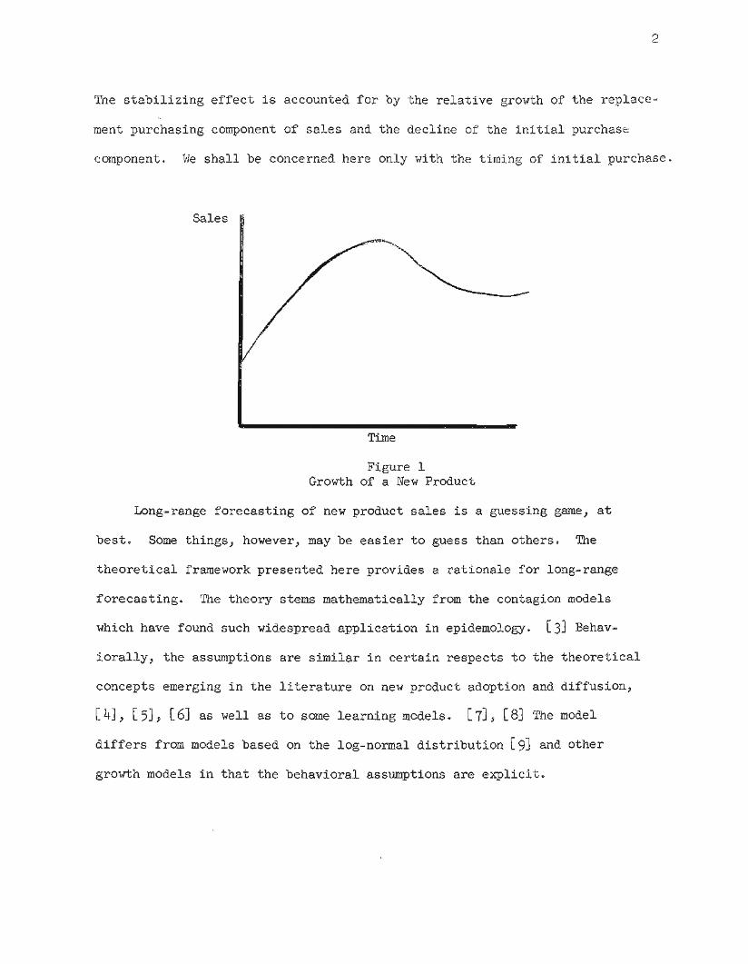
The stabilizing effect is accounted for by the relative growth of the replace-

ment purchasing component of sales and the decline of the initial purchase

component. We shall be concerned here only with the timing of initi~l purchase.

Sales ..

Time

Figure 1.Growth of a New Product

Long-range forecasting of new product sales is a guessing game, at

best. Some things, however, may be easier to guess than others. The

theoretical framework presented here provides a rationale for long-range

forecasting. The theory stems mathematically from the contagion models

which have found such widespread application in epidemology. [3J Behav-

iorally, the assumptions are similar in certain respects to the theoretical

concepts emerging in the literature on new product adoption and diffusion,

[4J, [5J, [6Jas well as to some learning models. [7J, [8J The model

differs from models based on the log-normal distribution [9J and other

growth models in that the behavioral assumptions are explicit.

3

'Ihe Theory of Adoption and Diffusion

The theory of the adoption and diffusion of new ideas or new products

by a social system has been discussed at length by Rogers. [4] This

discussion is largely literary. It is therefore not always easy to separate

the premises of the theory from the conclusions. In the discussion which

follows an attempt will be made to outline the major ideas of the theory as

they apply to the timing of adoption.

Some individuals decide to adopt an innovation independently of the

decisions of other individuals in a social system. We shall refer to these

individuals as innovators. We might ordinarily expect the first adopters

to be innovators. In the literature, the following classes of adopters are

specified: . (1) Innovators, (2) Early Adopters, (3) Early Majority, (4) Late

Majority, and (5) Laggards. This classification is based upon the timing of

adoption by the various groups.

Apart from innovators, adopters are influenced in the timing of adop-

tion.by th~ pressures of the social system, the pressure increasing for

later adopters with the number of previous adopters. In the mathematical

formulation of the theory presented here we shall aggregate groups (2)

through (5) above and define them as imit_e.tors. Imitators, unlike inno-

vators, are influenced in the timing of adoption by the decisions of other

members of the social system. Rogers defines innovators, rather arbitrarily,

as the first two and one-half percent of the adopters. Innovators are

described as being venturesome and daring. They also interact with other

innovators. When we say that they are not influenced in the timing of

purchase by other members of the social system, we mean that the pressure for

4

adoption, for this group, does not increase with the growth of the adoption

process. In fact, quite the opposite may be true.

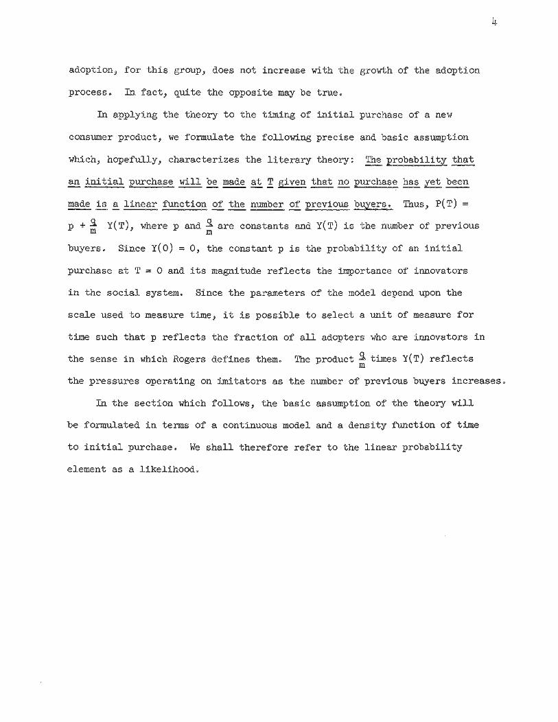
In applying the theory to the timing of initial purchase of a new

consumer product, we formulate the following precise and basic assumption

which, hopefully, characterizes the literary theory: The probability that

~ initial purchase ~ ~ ~ !i!given ~ ~ purchasehas yet ~. ,

~ ~ !!. linear function ~ ~ number ~ previoUs buyers. Thus, p(T) =

p +.9. yeT), where p and .9.are constants and yeT) is the number of previousm m

buyers. Since Y(O) = 0, the constant p is the probability of an initial

purchase at T = ° and its magnitude reflects the importance of innovators

in the social system. Since the parameters of the model depend upon the

scale used to measure time, it is possible to select a unit of measure for

time such that p reflects the fraction of all ad?pters who are innovators in

the sense in which Rogers defines them. The product .9.times yeT) reflectsm

the pressures operating on imitators as the number of previous buyers increases.

In the section which follows, the basic assumption of the theory'will

be formulated in terms of a continuous model and a density function of time

to initial purchase. We shall therefore refer to the linear probability

element as a likelihood.

5

Assumptions and the Model

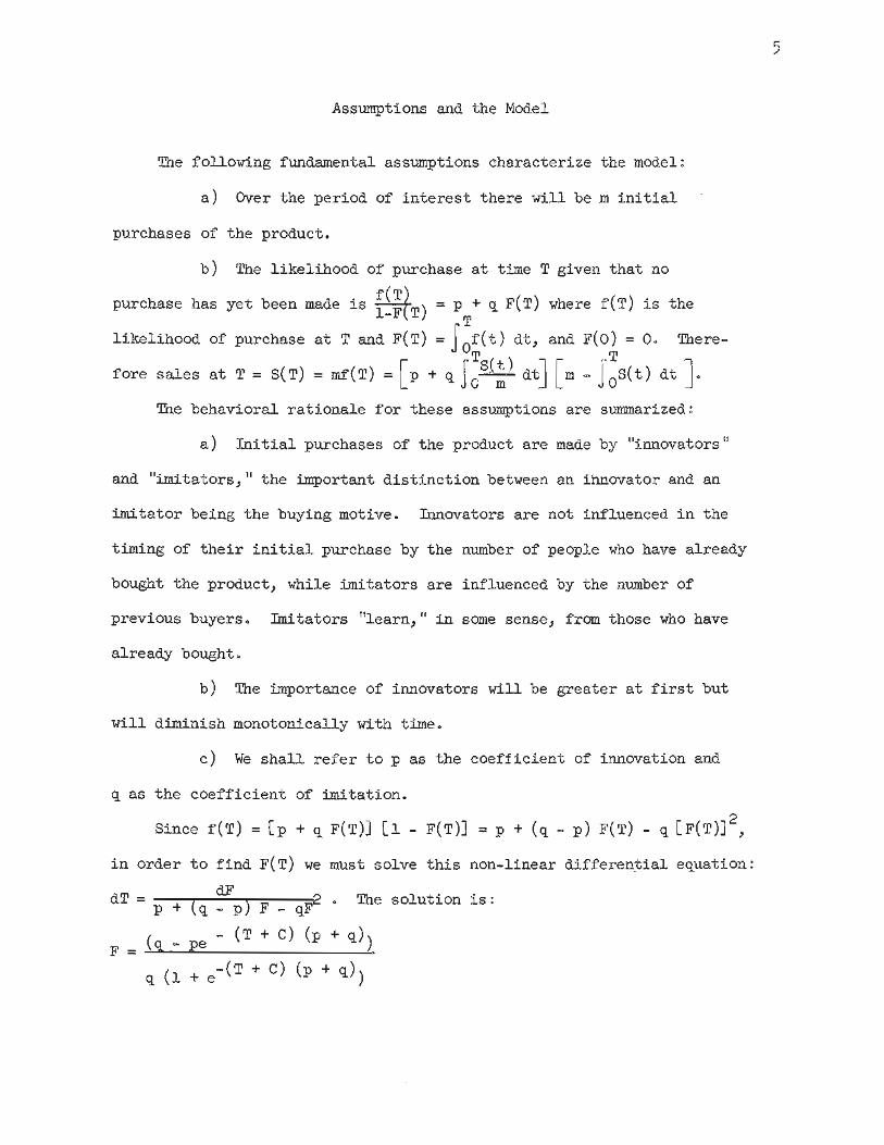
The following fundamental assumptions characterize the model:

a) Over the period of interest there will be mini tial

purchases of the product.

b) The likelihood of purchase at time T given that no

purchase has yet been made is i~~tT) :: p T+ q F(T) where f(T) is the

likelihoodof purchase at T and F(T) = S Of(t) dt, and F(O) = O. There-

[ JTs(t)

J [

('T

]fore sales at T = SeT) = mr(T) = p + q o~ dt m - j OS(t) dt .The behavioral rationale for these assumptions are summarized:

a) Initial purchases of the product are made by "innovators"

and "imitators," the important distinction between an ihnovator and an

imitator being the buying motive. Innovators are not influenced in the

timing of their initial purchase by the number of people who have already

bought the product, while imitators are influenced by the number of

previous buyers. Imitators "learn," in some sense, from those who have

already bought.

b) The importance of innovators will be greater at first but

will diminish monotonically with time.

c) We shall refer to.p as the coefficient of innovation and

q as the coefficient of imitation.

Since f(T) = [p + q F(T)] [1 - F(T)] = P + (q - p) F(T) - q [F(T)]2,

in order to find F(T) we must solve this non-linear differen~ial equation:

dT = + ( dF) F F2. The solution is:p q-p -q

( - (T+ C) (p + q) .)F = q - pe

q (1 + e-(T + C) (p + q))

6

Since F(O) = 0, the integration constant may be evaluated:

-c _ 1- I' + q Ln (qjp)

and F(T) = (1 - e - (p + q) T)

(_I (I'+ q) TY./pe + 1)

f(T) = (I' + q)2p.

e - (I' + q) T

(I' + q) T

(qjpe +. 1)2

, and

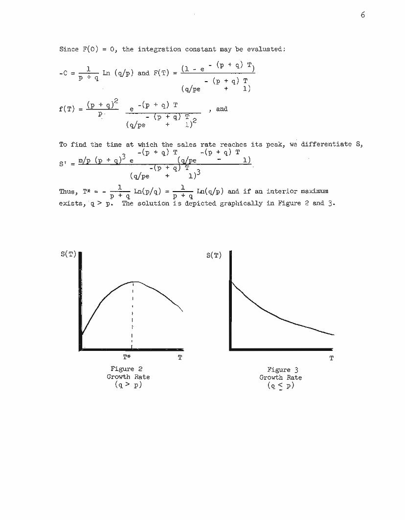
To find the time at which the sales rate reaches its peak, we differentiate S,

-(1"+ q) T -(I'+ q) T

S' = m e - 1)- I' T

(qjpe 1)3

Thus, T* = - .~ Ln(p/q) .= ~ Ln(qjp)and if an interiormaximumI' q I' q

exists, .q > p. The solution is depicted graphically in Figure 2 and 3.

SeT) SeT)

T*

Figure 2Growth Rate

(q> 1')

T T

Figure 3Growth Rate

(q "S 1')

7

We note thatS( T*) = m(p + q)2T

and Y(T*) =J S(t ) dt =m(q - p)° 2q'

Since for successful new products the coefficient of imitation will

ordinarily be much larger than the coefficient of innovation, sales

is approximately one-half m. We note also that the expected time

to purchase, E(T), is ~ Ln~ ; ~ .

The Discrete Analogue

The basic model is:2

SeT) = pm + (q - p) yeT) - qjm Y (T).

In estimating the parameters p,q, and m from discrete time series

data we use the following analogue: ST = a + bYT _ 1 + c~ _ 1 ' T =2,3...T - 1

T, and YT _ 1: t ~ 1 St = cumulative 'sales throughwhere: ST ~ sales at

period T-l. Since a estimates pm, b estimates q-p, and c estimates

-qjm: -mc = q, aim = p.2

Then q - p = -mc -aim = b, and c m + bm + a = 0, or m =

+J 2 4-b- b - ca2c

and the parameters p, q, and m are identified. If we write S(YT _ 1)dS

and differentiate with respect to YT _ l' dyTT --b m(q - p)

Y* = 2c = 2qT - 1Setting this equal to 0,

b2 b2 m(p + q)2a-2C+4C= 4q

= b + 2cYT _ l'1

= Y(T*), and S (y* ) =T T - 1

= S(T*) . Therefore, the maximum value of S as

a function of time coincides with the maximum value of S as a function of

cumulative sales.

Regression Analysis

In order to test the model, regression estimates of the parameters

were developed using annual time series data for eleven different consumer

8

durables. The period of analysis was restricted in every case to include

only those intervals in which repeat purchasing was not a factor of impor-

tance. Table 1 displays the regression results.

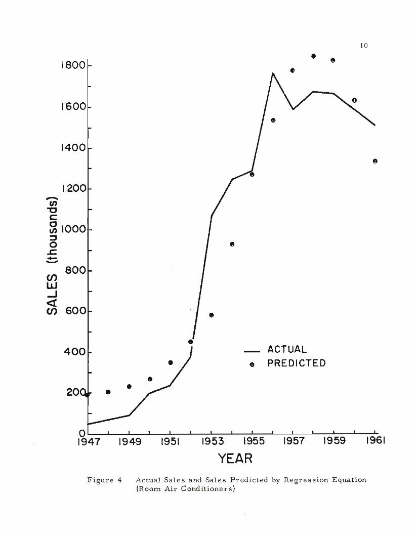
The data appear to be in g~od agreement with the model. The R2 values

are reasonably high and the parameter estimates seem reasonable for the

model. Figures 4, 5, and 6 show the actual values of sales and the values

predicted by the regression equation for three of the products analyzed.

For every product studied the regression equation describes the general

trend of the time path of growth very well. In addition, the regression

equation provides a very good fit with respect to both the magnitude and

the timing of the peaks for all of the products. Deviations from trend

are largely explainable in terms of short-term income variations. This

is especially apparent in Figure 5, where it is easy to identify recessions

and booms in the years of sharp deviations from trend.

TableI

ProductPeriodCovered

Growth Model Regression Results For Eleven Consumer Durable Products

~ ~ ~ R2 ~ ~3, (,,,-7, c~ ~

Ac

"7ii\m3

p q

Data Sources: Economic Almanac, Statistical Abstracts of the U.S.,

Electrical Merchandising, and Electrica1JMerchaDd1Sing ~.

\0

, J - . - ,

Electric

Refrigerators 1920-1940 104.67 .21305 -.053913 .903 1.164 6.142 -2.548 40,001 .0026167 .21566

Home1946-1961 308.12 .15298 -.071868 .742 4.195 4.769 -3.619 21,973 .018119 .17110

Freezers

Black and WhiteTelevision 1946-1961 2,696.2 .22317 -.025957 .576 3.312 3.724 -3.167 96,717 .027877 .25105

Water Softeners 1949-1961 .10256 .27925 -512.59 .919 3.593 8.089 -6.451 5,793 .017103 .29695

Room AirConditioners 1946-1961 175.69 .40820 -.24777 .911 1.915 8.317 -6.034 16,895 .010399 .41861

Clothes Dryer 1948-1961 259.67 .33968 -.23647 .896 2.941 7.427 -5.701 15,092 .017206 .35688

PowerI.awnmowers 1948-1961 410.98 .32871 -.075506 .932 1.935 7.408 -4.740 44,751 .0091837 .33790

Electric Bed

Coverings 1949-1961 450.04 .23800 --031842 .976 3.522 6.820 -1.826 76,589 .005876 .24387

AutomaticCoffee Makers 1948-1961. 1,008.2 .28435 -.051242 .883 3.109 6.186 -4.353 58,838 .017135 .30145

Steam Irons 1949-1960 1,594.7 .29928 -.058875 .828 3.649 5.288 -4.318 55,696 .028632 .32791

Record Players 1952-1961 543.94 .62931 -.29817 .899 1. 911 5.194 -3.718 21,937 .024796 .65410

enIJ.J...J«en

..

20..

o1947 1949 1951

10

. .

.

.

- ACTUALPREDICTED.

1953 1955

YEAR1957 1959 1961

Figure 4 Actual Sales and Sales Predicted by Regression Equation(Room Air Conditioners)

1200

110

1000

11

500

400

1947 1949

- ACTUAL. PREDICTED

1951 1953 1957 1959 19611955

YEAR

Figure 5 Actual Sales and Sales Predicted byRegression Equation(Home Freezers)

900(/)-cc:0 8001 I.(/)::J I .0.c

b

enLLI...J«en 60

12

8000

7000

.

6000

1000

- ACTUAL'. PREDICTED

1947 1949 1951 1953 1955

YEAR1957 1959 1961

Figure 6 Actual Sales and Sales Predicted byRegression Equation(Black & White Television)

.....-.-

5000c::c(/):I

4000..........- - - .. .CJ)

3000 r- .«CJ)

2000

13

Model Performance

The performance of the regression equation relative to actual sales is a,

relatively weak test of the modei.tsperformance since it

comparison of the regression equation estimates with the

test is the performance of the basic model with time as

amounts to an .~ ;E9st

data. A much stronger

the vari3ble and control~

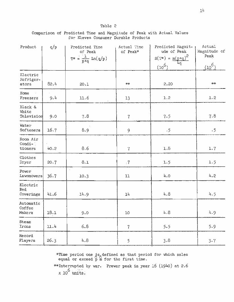
ling parameter values as determined from the regression estimates. Table 2

provides a comparison of the model's prediction of time of peak and magnitude of

peak for the eleven products studied.

Since, according to the model S(O) = pm, we identify time period I as that

period in which sales equal or exceed ~ for the first time. It is clear from

the comparison shown in Table 2 that the model provides good predictions of the-

timing and magnitude of the peaks for all eleven products studied.

In order to determine the accuracy with which it would have been possible

to "forecast" period sales over a long-range interval with prior knowledge of

the parameter values, the regression p.stimates of the parameters were substituted

in the basic model,

S(T)c - (p + q) T

( /(p + q)

q pe +

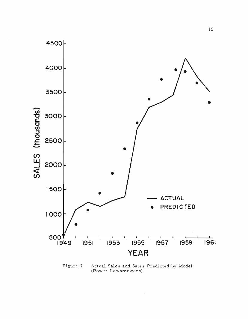
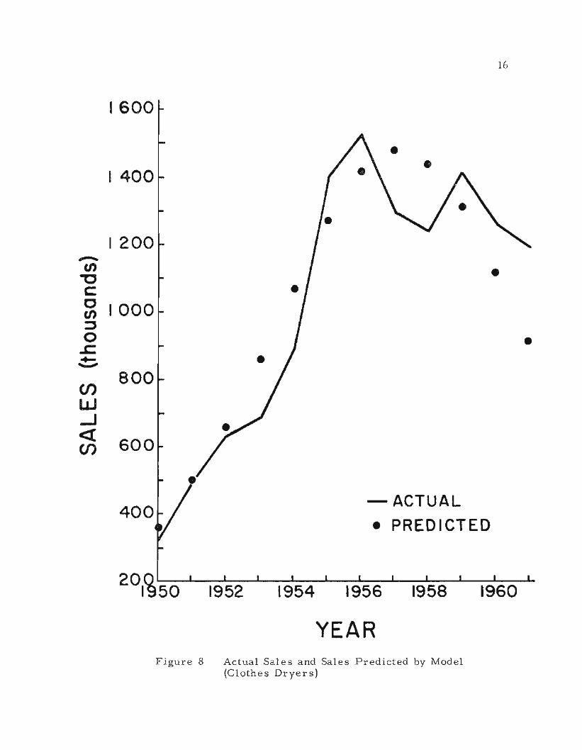
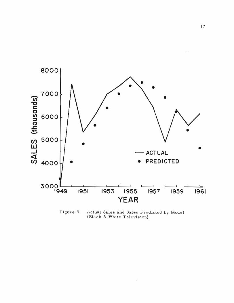
arid sales estimates generated for each of the products for each year indicated

in the intervals shown in Table 3. In most cases the model provides a good

fit to the data. Even in the few instances of low 1'2values, the model provides

a good description of the general trend of the sales curve, the deviations from

trend being sharp, but ephemeral. Figures 7, 8, and 9 illustrate the predicted

and actual sales curves for three of the products.

14

Table 2

Comparison of Predicted Time and Ma~tude of Peak with Actual Valuesfor Eleven Consumer Durable Products

*Time period one ASAdefined as that period for which salesequal or exceed p m for the first time.

**Interrupted by war. Prewar peak in year 16 (1940) at 2.66 ,,'.--, '

x 10 Uriits;

Product qjp Predicted Time Actual Time Predicted Magnit- Actual

of Peak of Peak* ude, of Peak, " Magni tude of, ,. "1 2 Peak

T* Ln(qjp) S(T*) =p+q

(106)(106) q

Electric

Refriger-ators 82.4 20.1 ** 2.20 **

Home ' ' ..'

Freezers 9.4 11.6 13 1.2 1.2.

Black &WhiteTelevisior 9.0 7.8 7 7.5 7.8

WaterSofteners 16.7 8.9 9 .5 .5

Room AirCondi.. "

..,

tioners 40.2 8.6 7 1.8 1.7

Clothes

Dryer 20.7 8.1 :1 1.5 1.5

PowerLawnmowers 36.7 10.3 11 4.0 4.2

ElectricBed

Coverings 41.6 14.9 14 4.8 4.5"

AutomaticCoffeeMakers 18.1 9.0 10 4.8 4.9,-

SteamIrons 11.4 6.8 7 5.5 5.9

RecordPlayers 26.3 4.8

I

5 3.8 3.7

1953 1955 1957

YEAR

4500

4000

3500

----.

~ 3000ccU)::Jo

.s::. 2500

...'--'

(J)

~ 2000«(J)

.

1500

1000

.

50019~9 1951

15

.

- ACTUAL. PRED 1CTED

1959 1961

Figure 7 Actual Sales and Sales Predicted by Model(Power Lawnrnowers)

1600

1400

16

400- ACTUAL. PREDICTED

1954 1956 1958 1960

YEARFigure 8 Actual Sales and Sales Predicted by Model

(Clothes Dryers)

1200......-.fn-c rc:

I

Cfn 1 000

. .

0.s=

L

0I

en800

.

IJJ-I<ten 600

8000

7000f/)

"'CCC

~ 6000o

.s::;+-,.

en 5000ILl...J«en 4000

30001949

17

. .

.- ACTUAL. PRED1 CTED

1951 1953 1955 1957

YEAR

1959 1961

Figure 9 Actual Sales and Sales Predicted by Model(Black & White Television)

1$

It would eppear fair to conclude that the data are in generally good

agreement with the roodel. 'l"hemodel has, then, in some sense, been "tested"

and verified, He may now claim to know something about the phenomenon we

set out to explore. The question is, however, will this knowledge be useful

for purposes of long-range forecasting?

Long-Range Forecasting

There are two cases worth considering in long-range forecasting:

the no-data case and the limited-data case. For either of these possibilities

one may well ask: is it easier to guess the sales curve for the new product

or easier to guess the parameters of the model? No attempt will be made here

to answer this question, in general, but it does seem likely that for some

products it would be possible to make plausible guesses of the parameters.

Analysis of the potential market and the buying motives should make it possible

to guess at m, the size of the market, and of the relative values of p and q,

the latter guess being determined by a;:b'0nsideration ofbu:.yiJilgmotives;.. If

the sales curve is to be determined by means other than the model suggested

in this paper, the implications of this forecast in terms of the parameters

of the model might be useful as a test of the credibility of the forecast.

In order to illustrate the forecasting possibilities in the limited data

case, we shall develop a forecast for color television set sales. In prin-

ciple, since there are three parameters to be estimated, some kind of esti-

mate is possible with only three observations if the first of these obser-

vations occurs at T = O. Any such estimate should be viewed with some

skepticism, however, since the parameter estimates are very sensitive to small

variations in the three observations. Before applying estimates obtained from

19

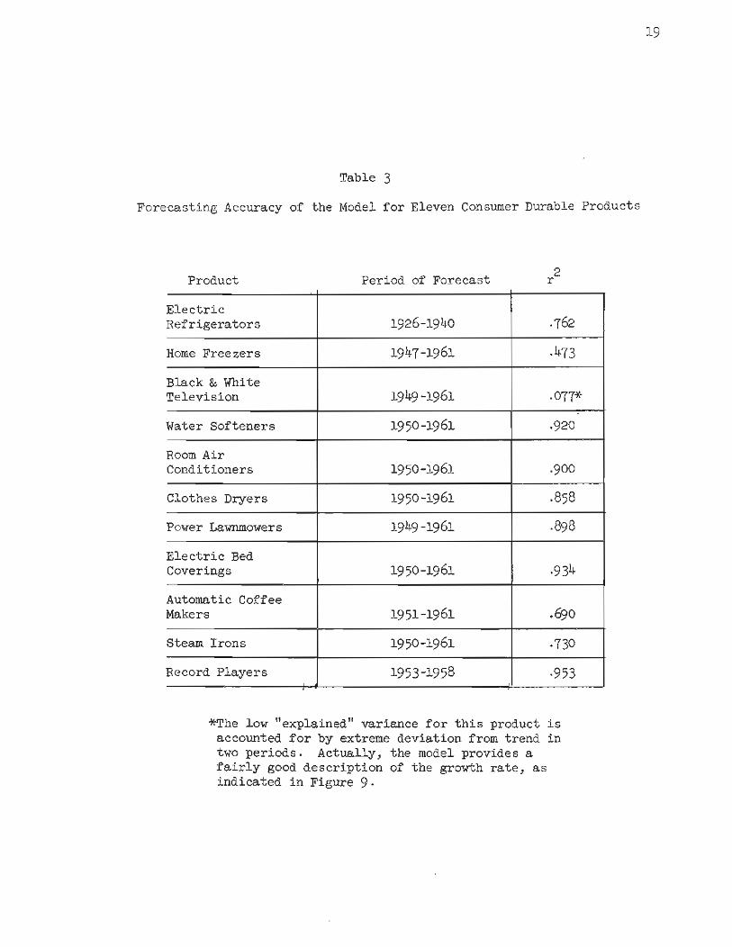
Table 3

Forecasting Accuracy of the Model for Eleven Consumer Durable Products

Product Period of Forecast2r

*The low "explained" variance for this product is

accounted for by extreme deviation from trend in

two periods. Actually, the model provide s a

fairly good description of the growth rate, asindicatedin Figure9.

Electric

Refrigerators 1926-1940 .762

Home Freezers 1947-1961 .473

Black & WhiteTelevision 1949 -1961 .077*

.

Water Softeners 1950-1961 .920.

Room Air

Conditioners 1950-1961 .900

Clothes Dryers 1950-1961 .858

Power Lawnmowers 1949 -1961 .898

Electric Bed

Coverings 1950-1961 .934

Automatic Coffee

Makers 1951-1961 .690

Steam Irons 1950-1961 .730

Record Players 1953-1958 .953

20

a limited number of observations, the plausibility of these estimates should

be closely scrutinized.

T-l

In substituting ~ St int=ocontinuous model, a certain bias was introduced.

,Tthe discrete analogue for! Set) dt in the

VoThis bias is mitigated when

there are several observations, but can be crucial when there are only a few.

Thus, the proper formulation of the discrete model, if ST = SeT) is: ST =

2 2 yeT)a + bk(T) YT _ 1 + ck (T) YT _ l' where k(T) = y-- . We note that for any

T = 1probability distribution for which~ a) f(x) = l/k [F (x + 1) = F(x)J, and b)

x-l

F(O) = 0, ~ f(t) = l/k F(x)ot=O

In particular, these two properties hold for the

x=l ()exponential distribution. Therefore, for this distribution ~ ~ = ko The

t=O f(t)

density function f(T) in the growth model developed in this paper is approx-

imately exponentialin characterwhen 1'1 and T aresmall0 ThUs, f (T) = !kapx

[F. (T+~) - F (T)]an~.= (p + q) . ForsmallvaluesofT weapx apx ( + )

[e p q - 1] 2

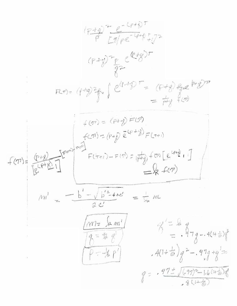
therefore write: ST = a + b'YT _ 1 + ct~ _ l' Where b' = kb, and c' = k C.

~t _'1£q_1 ~. pIThen m = l~t, q = .~1) and p =~. The value Of'(k for each of several

different values of p + q has been calculated and appears in Table 40

j"

I

b'~' -i 1/ ,-' j-, - ---1

~ =);;-- ~I i.' .~

).. Ji

d;;

..---

bJ i, Z.-- - J b -4~t.f- ' . --

~ c..,'

" - (j

q

~I .- x;.,f) ~

J ':: . '76 ~. 4(1-1i;)b

, 4(J-I- ~)6 ~ -. 97?+(=-0--..-

q -; , ~1,~fl:.'11)?--f.~ (l+l,Jt.0 ,~(l~~}

21

Table 4

Calculated Values O:f~k and (p + q)

(p + q)

-3.4.5.6.7.8.9

.85

.81

.77

.73

.69

.65

.61

On the basis o:f the relationship betweeny,k and (p + q) indicated in

I . 'f~I.'t! .97 q ITable 4: Ik = .97 - ·4 (p + q), q = ~ = , ..LI, (, ..L 1 Ie. \ ~ I , wheree =

.

qf d - ~ q = .97 p'.q '/p' = p, an p - q' 1 + .4 (1 + e )p'

\ve turn now to the :forecast o:f color teleVision set. sales. ..The :folloWing

data are available:

Sales(Millions o:f Units)

.71.352.50

Year

Solving the :following system o:f equations:

So = .7 = a

Sl = 1.35 = a + .7 b' + .49 c'

S2 = 2.50 = a + 2.05 b' + 4.20 c', we :find:

a' = .7, b' = .954, c' = -.0374,

m' = 26.2, q' = .96, pi = ,0267,

q = .67, p = .018, m= 37.4. .,

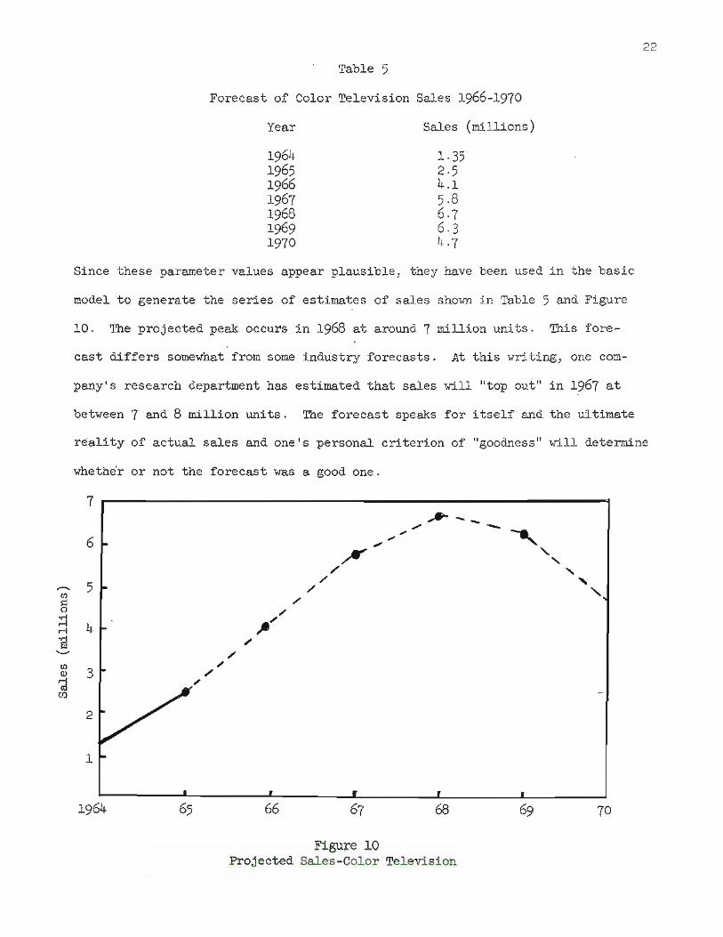
Table 5

Forecast of Color Television Sales 1966-1970

22

Year Sales (millions)

1964196519661967196819691970

1.352.54.15.86.76.34.7

Since these parameter values appear plausible, they have been used in the basic

model to generate the series of estimates of sales shown in Table 5 and Figure

10. The projected peak occurs in 1968 at around 7million units. This fore-

cast differs somewhat from some industry forecasts. At this writing, one com-

pany's research department has estimated that sales will "top out" iri1967 at

between 7 and 8 million units. The forecast speaks for itself and the ultimate

reality of actual sales and one's personal criterion of "goodness" will determine

whether or not the forecast was a good one.

7

1964 66 68

Figu;re 10Projected Sales-Color Television

" "" " , "

70

6

.......... 5tos::0'ri

4'B........

toQ) 3Mcd(J)

2

1

23

While this forecast was objectively determined in the sense that it was

derived from data, it is also based upon a subjective judgment of the plau-

sibility of the parameters. Since the parameter estimates are very sensitive

to small variations in the observations when there are only a few observations,

the importance of the plausibility test cannot be overemphasized.

Conclusion

The growth model developed in this paper for the timing of initial

purchase of new products is based upon an assumption that the probability of

purchase at any time is related linearly to the number of previous buyers.

There is a behavioral rationale for this assumption. The model implies

exponential growth of initial purchases to a peak and then exponential decay.

In this respect it differs from other new product growth models.

Data for consumer durables are in,good agreement with the model. Parameter

estimates derived from regression analysis when used in conjunction with the

model provide good descriptions of the growth of sales. From a planning

viewpoint, probably the central interest in long-range forecasting lies in

predictions of the timing and magnitude of the sales peak. The model provides

good predictions of both of these variables for the products to which it has

been applied. Insofar as the model contributes to an understanding of the

process of new product adoption, the model may be useful in providing a

rationale for long-range forecasting.

24 24

15

18

06

- ACTUAL. PREDICTED.

03 .

01 02 03 04 05 06

TIME PERIODS07 08 09 10

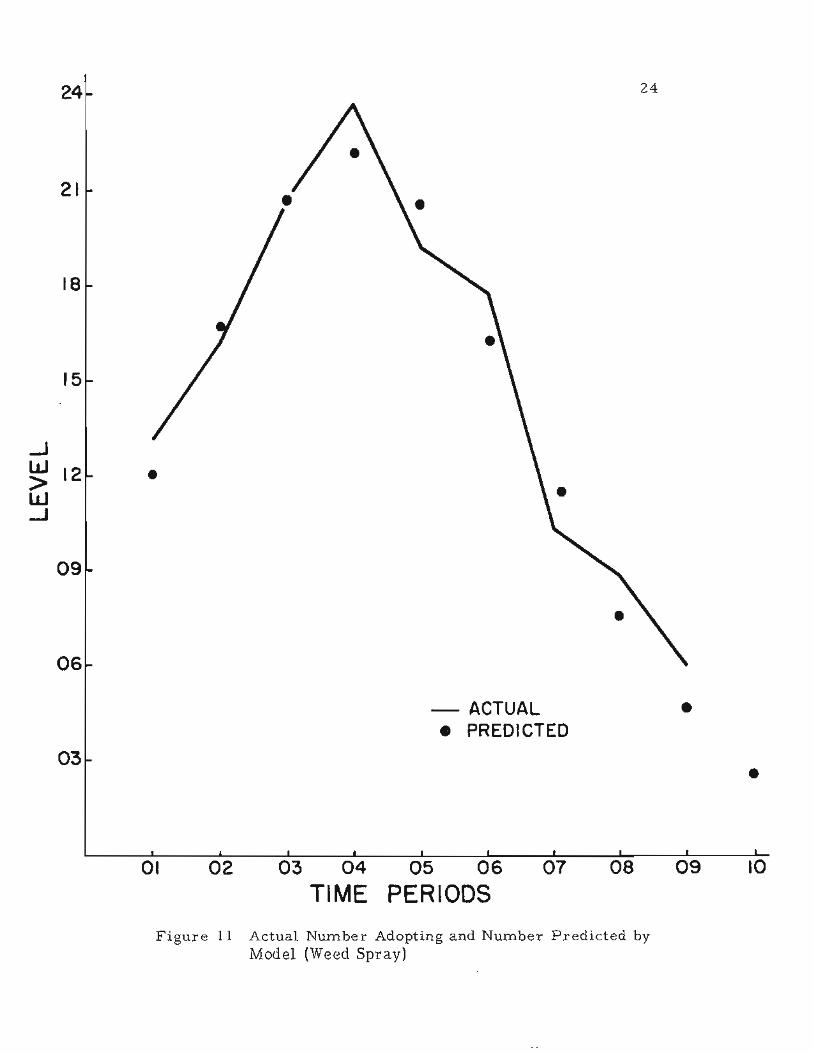
Figure 11 Actual Number Adopting and Number Predicted byModel (Weed Spray)

-

-'W 12 .>W..J

09

22.5

20.

1'7.5

15.0

12.51

JW>W

J IQO

'7.51

5.0

2.51

.

01 02 03

TIME

25

.

.

.".- ACTUAL. PREDICTED

04 05

PERIODS06 07 08

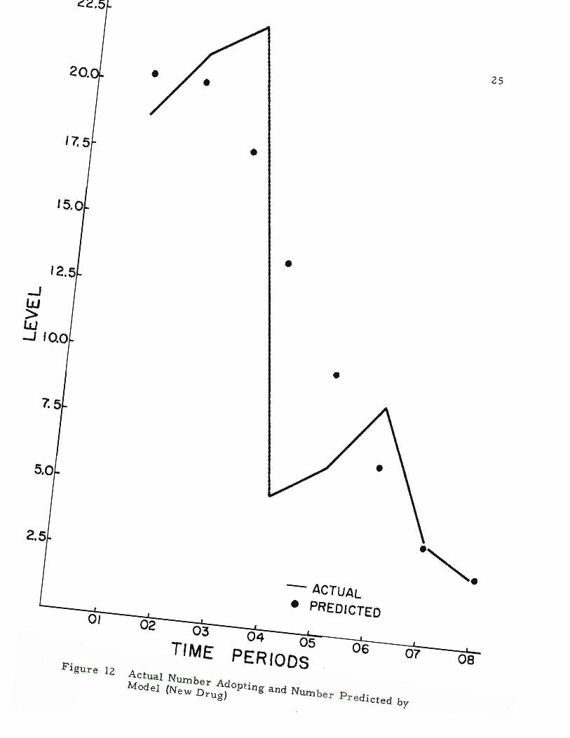
Figure 12 Actual Number Adopting and Number Predicted byModel (New Drug)

26

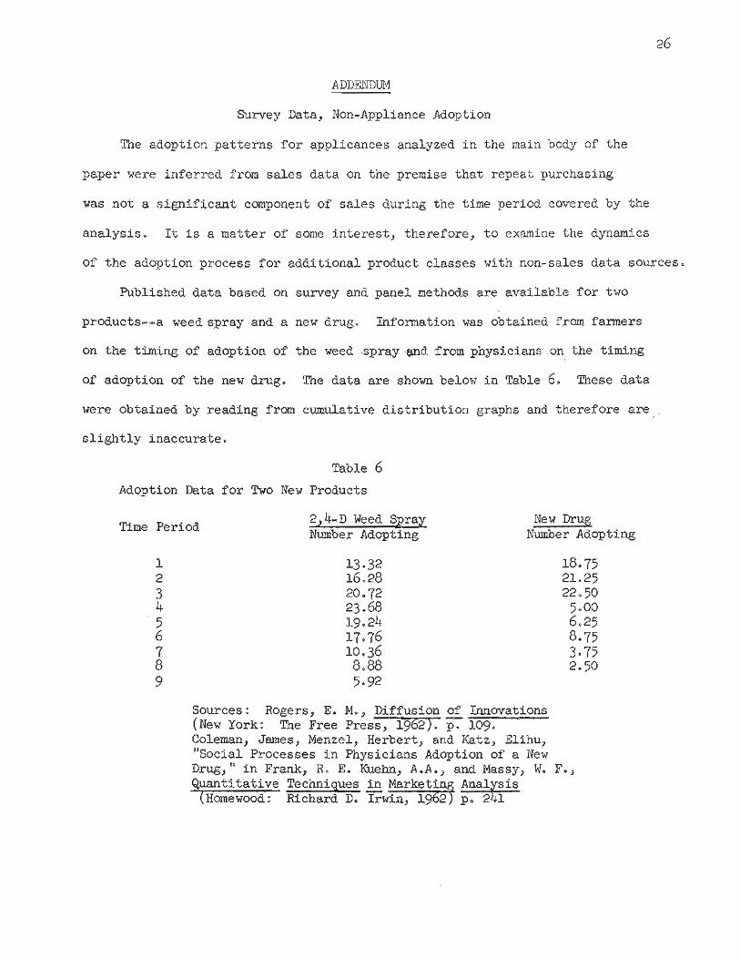
ADDENDUM

Survey Data, Non-Appliance Adoption

The adoption patterns for applicances analyzed in the main body of the

paper were inferred from sales data on the premise that repeat purchasing

was not a significant component of sales during the time period covered by the

analysis. It is a matter of some interest, therefore, to examine the dynamics

of the adoption process for additional product classes with non-sales data sources.

Published data based on survey and panel methods are available for two

products--a weed spray and a new drug. Information was obtained from farmers

on the timing of adoption of the weed ,spray ,~d'from physi:cians..on,the timing

of'adoption of the new drug. The data are shown below in Table 6. These data

were obtained by reading from cumulative distribution graphs and therefore are

slightly inaccurate.

Table 6Adoption Data for Two New Products

Sources: Rogers, E. M., Diffusion of Innovations(New York: The ~ee Press, 1962). p:-109.Coleman, James, Menzel, Herbert, and Katz, Elihu,"Social Processes in Physicians Adoption of a NewDrug," in Frank, R. E. Kuehn, A.A., and Massy, W. F.,

Quantitative Te'chniques~ Marketing AnalksiS(Homewood: Richard D. Irwin, 1962) po 2 1

Time Period 2,4-D Weed Spray New Drug

Number Adopting Number Adopting ,

1 13.32 18.752 16.28 21.253 20.72 22.504 23.68 5.005 19.24 6.256 17.76 8.757 10.36 3.758 8.88 2.509 5.92

The results of the regression analysis are summarized in Table 7 and

Figures 11 and 12. The density function of time to initial purchase is

again unimodel and the model adequately describes the data.

Table 7

Parameter Estimates For a Weed spray and a New Drug

Parameters Weed spray New D

a 8.04387 17.81431b .44472 .189229c -.00346 -.003277m 144.1 107.07q .4998 .35086

P2 .0558 .16638

R2 .953 .827r .958 .791

28I

References

1. Haines, G. H., Jr., "A Theory of Market Behavior After Innovation,"Management Science', No.4, Vol. lO, July, 1964. .

2. Fourt, L., A. and WoodlQck, J. W., "Ea:r~y Prediction of Market Successfor New Grocery Products," Journal of Marketing, No.2, Vol. 26,October, 1960.

3. Bartlett, M. S.. Stochastic Population Models in Ecolo

4. Rogers, E. M., Piffusionof Innov)tt:ions, New York: The Free Press, 1962.

5 . King, C" W., "AQ.option and Diffusion Research in Marketing: An Overview,"in Science, Technology and Marketing, 1966 Fall Conference of theAmerican Marketing Association, Chicago, 1966. (

6. Katz, E. and Lazarsfeld, F., Personal Inflttence, New Yor~: The Free Press,1955.

7. Rashevsky, N., Mathematical Biolo~ of Social Behavior, Chicago: The, University Press, 1959 "

8. Bush, R. R. and, Mostel;Ler, F., Stochastic Models for Learning, NewYork: Wiley, 1955.

9. Bain, A. D., The Growth of Television Owners:Q.ipin the United Kingdom,A Lognormal Model, Cambridge;: The University Press, 19

10, Dernburg , T., F ., "Consumer Response to Innovation: Television," inStudies in Household Economic Behavior, Yale Studies in'Economics,Vol. 9, New Haven, Connecticut: Yale, 1958. '

.. .11... Massy, W. F., "Innovation and Market Penetration,:' Ph,D. Thesis,

Massachusetts Institute of Technology, 1960, Cambr1dge, Massachusetts.

l2. Mansfield, E., "Techno1.ogical Change and the Rate of Imitation,"Econometrica, No.4, Vol. 29, October, 1961.

13. Pessemier, E. A., .NewProduc,t Decisions, An AnalMcGraw-Hill, 19

roach, New York:

APPENDIX

C ;_J~L.:::;PllliDICTION ANALYSIS-REGRESSIONCOEFFICIENTS 29DIMENSIONTITLE (80), S( 50) , IDNUM(50) , ACTSAL(50 )DATADOLLAR,/lH$,lHb /

1 READ(5,100) TITLE -WRITE(6,101) TITLESENT=BLANK

READ(5,102) A,B,C,N0=(~B-SQRT(B**2-4.*A*C»/(2.* C)P-A/OQ=-O*CK=lMM=ODO 7 I=l,NT=FLOAT(I) .S(K)=(0*(P+Q)*(EXP«-P-Q*T)/«Q(.P*EXP«-P-Q)*T)+1.)**2»IF(SENT .EQ.DOLLAR) GO TO 6READ(5,103) IDNUM(K),ACTSAL(K),SENTMM=K

6 IF(K.EQ.l.AND.ACTSAL(K) .LT.A) GO TO 7K=K+l

7 CONTINUEWRITE(6,104) O,P,QWRITE( 6,105)DO 8 I=l,MMWRITE(6,106) I, IDNUM(I),S(I),ACTSAL(I)

8 CONTINUENN=MM+lIDNUMP=IDNUM(MM)K=K-lDO 9 I=NN,KIDNUMP=IDNUMP+lWRI~(6,107) I,IDNUMP,S(I)

9 CONTINUESUMSQD=O.0SUM=O.OSUMSQ=O . 0

DO 10 I=l,MMSUMSQ=SUMSQ+(S(I)-ACTSAL(I»**2

10 SUM=SUM+ACTSAL(I)DO 11 I=l,MM

11 SUMSQD=SUMSQD+(ACTSAL(I)-(SUM/FLOAT(MM»)**2RSQ-l. -(SUMSQ/SUMSQD)

WRm:(6,lOB) RSQGO TO 1

100 FORMAT(80Al)101 FORMAT(lHl,19R PRODUCTANALYZED. , 80Al)102 FORMAT(3F20.8,12)103 FORMAT(14,FI0.3,65X,Al)104 FORMAT(lH ,13H COEFFICIENTS,10X,4R M= ,FI0.3,10X,4H P= ,F12.8,10X,

l4R Q= ,F12.8///)105 FORMAT(iH ,13H SALES PERIOD, lOX, 5R YEAA,lOX, lOR EST-SALES, lOX, lOR

lACT-SALES ),106 FORMAT(lH ,llX,'12,llX,1~,llX,F9.3,1+X,F9.3)107 FORMAT(lH ,llX;12,llX,14,llX,F9.3)108 FORMAT(lH ,13R R S~ARED = ,F7.5),

END .$DATA

30

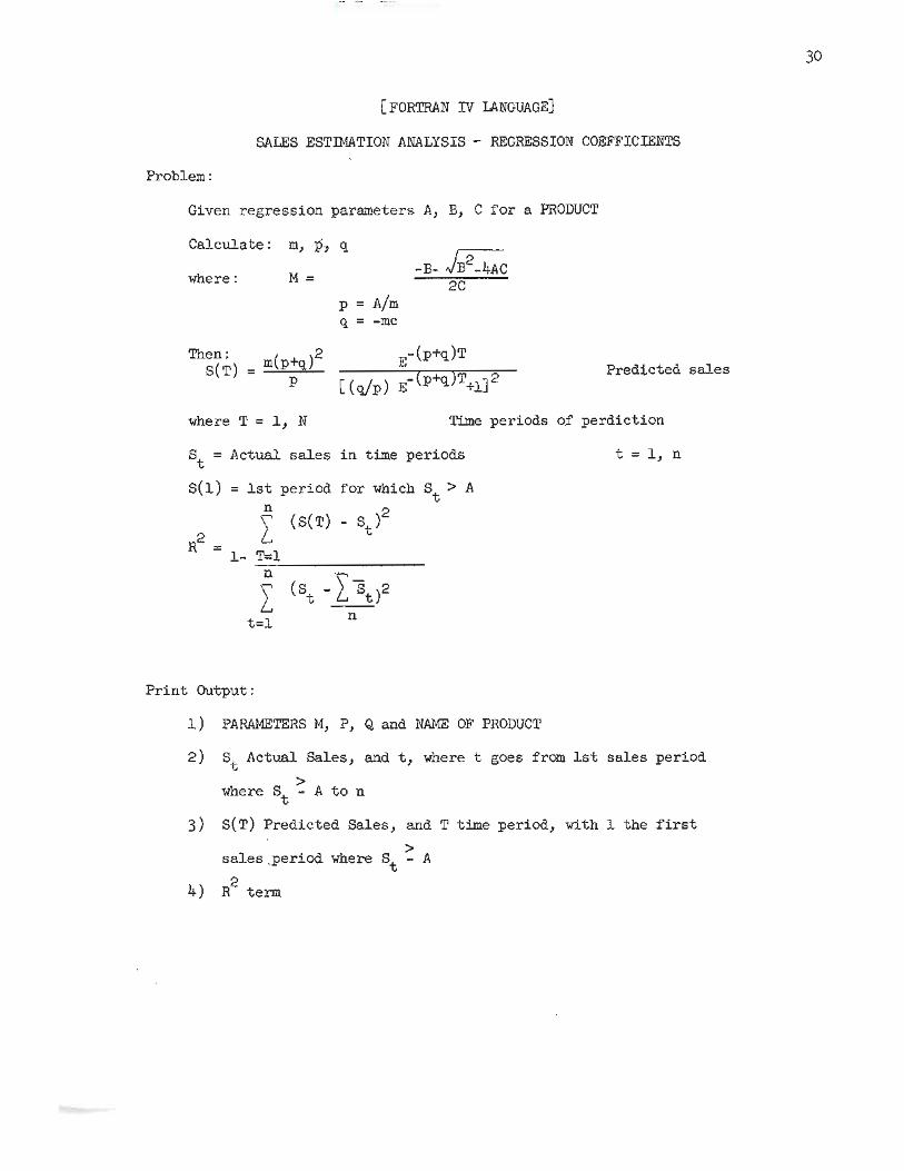
[FORTRAN IV LANGUAGE]

SALES ESTIMATIONANALYSIS- REGRESSIONCOEFFICIENTS

Problem:

Given regression parameters A, B, C for a PRODUCT

Calculate: m, 15, q

where: M =

p = Aimq = -mc

Then: 2S(T) = m(p+q) E-(P+q)T

p [(qfp) E-(p+q)T+J.]::?Predicted sales

where T = 1, N Time periods of perdiction

St = Actual sales in time periods t = 1, n

S(l) = 1st period for which

f (S(T) - St)2

S > At

Print Output:

1) PARAMETERSM, P, Q and NAMEOF PRODUCT

2) St Actual Sales, and t, where t goes from 1st sales per:i,od> .

where St - A to n

3) S(T) Predicted Sales, and T time period, with 1 the first

1 . >sa eS.,perJ.od where St - A2

4) R term

31

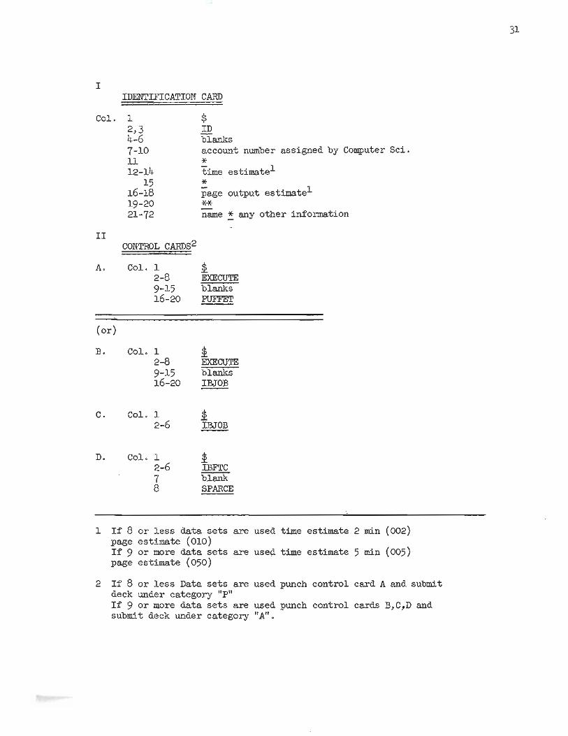
1 If8 or less data sets are used time estimate 2 min (002)page estimate (010)If 9 or more data sets are use~ time estimate 5 min (005)page estimate (050)

2 If 8 or less Data sets are used punch control card A and submitdeck under category "P"If 9 or more data sets are used punch control cards B, C.,D andsubmi t deck under category "A".

IIDENTIFICATIONCARD

Col. 1 $2,3 .m4-6 blanks7-10 account number assigned by Computer Sci.11 *12-14 time estimate1

15 *16-18 page output estimate119-20 **21-72 name .! any other information

IICONTROL CARDS2

A. Col. 1 !2-8 EXECUTE9-15 blanks16-20 PO'FFET

(or)

B. Col. 1 !2-8 EXECUTE9-15 blanks16-20

C. Col. 1 !2-6

D. Col. 1 !2-6 IBFTC7 ;;-raDk8 SPARCE

32

IIIDATA CARDS

A. TITLE CARD

Name of product to be analyzed is punched on this cardCol 1-30 may be used with any data to define name.

B. COEFFICIENTS.AND LIMIT CARD

Co1.Co1.Co1.Co1.

1-2021-4041-6061-62

VALUE OF COEFFICIENT AVALUEOF COEFFICIENT BVALUE OF COEFFICIENT CMAXIMUMNUMBEROF SALES PERIODS FOR WHICHPREDICTION WILL BE MADE (N ~ 50)

Values of A,B,C may be numbers whose total length each is 19 or lessdigi ts with 8 or less digits to right of decimal point. Decimal Pointmust be punched.

N is a two digit number between 01-50. Decimal Point ~ E.2!~ punched.

C. ACTUALSALES CARD(S)

Col. 1-4 IDENTIFICATION NUMBERFOR SALESVALUE(ALL four digits punched (0001»

Co1. 5-14 VALUEOF ACTUALSALES FOR PARl'ICULARIDENTIFICATIONNUMBER

Valu~ of Actual sales may have up to 9 digits or less, with3 or less digits to right of decimal point. Decimal point~ 'be punched.

Col. 80 blank or !A ! in Col 80 signals the end of a data set. This char-acter must be punched on the Last ACTUAL SALES CARD for~given~set. - ---

The number of ACRTALSALESCARDS must not exceed 50 andmust be less than equ'BI""'tO N (Specified in data card B)

IV

33

ORDER OF CARDS

DataDeck

1-2.3.

~:U.

IDENTIFICATION CARD

CONTROL CARD(S)SALES PREDICTION ANALYSIS - PROGRAMDECK

TITLE CARD (A)COEFFICIENTSANDLIMIT CARD (B)

ACTUAL SALES CARD(S) (C) [WITH! IN COL80 OF LASTCARD]

Items 4-6 may be repeated any number of times if more than one data

set is used. See Notes (1) and (2) for proper control cards andjob category.

PURDUEUNIVERSITY

KRANNERT SCHOOLOF INDUSTRIALADMINISTRATIONINSTITUTE PAPER SERIES

(Continued from inside front cover)

105. Michael J. Driver and Siegfried A. Streufert, THE "GENERAL INCONGRUITY ADAPTATION LEVEL" (GIAL) HYPOTHESIS:AN ANAL YSIS AND INTEGRA TION OF COGNITIVE APPROACHES TO MOTIVA TION.

106. William H. Starbuck, THE HETEROSCEDASTIC NORMAL.

107. John J. Sherwood and John R. P. French, SELF-ACTUALIZATION AND SELF-IDENTITY THEORY.*

108. Richard E. Walton and Robert B. McKersie, BEHAVIORAL DILEMMAS IN MIXED MOTIVE DECISION-MAKING.#109. Stanley Reiter and Donald B. Rice, DISCRETE OPTIMIZING SOLUTION PROCEDURES FOR LINEAR AND NONLINEAR

INTEGER PROGRAMMING PROBLEMS.#

110. John J. Sherwood, SELF-REPORT AND PROJECTIVE MEASURES OF ACHIEVEMENT AND AFFILIATION.#*111. Ronald Kochems, AN APPLICATION OF MUL TIPLE DISCRIMINANT ANAL YSIS.

112. John A. Shaw, THE THEORY OF CONSUMER RATIONING, PARETO OPTIMALlTY, AND THE U.S.S.R.113. R. K. James, W. H. Starbuck and D. C. King, A STUDY OF PERFORMANCE IN A BUSINESS GAME _ REPORT 1.114. Michael J. Driver, Purdue University, and Siegfried Streufert, Rutgers-The State University, TH E GEN ERAL INCONGRUI TY

ADAPTATION LEVEL (GIAL) HYPOTHESIS: AN ANALYSIS AND INTEGRATION OF COGNITIVE APPROACHES TOMOTIVATION.

115. Frank M. Bass and Ronald T. Lonsdale, AN EXPLORATION OF LINEAR PROGRAMMINGIN MEDIA SELECTION. *116. Frank M. Bass, THE DYNAMICSOF MARKET SHAREBEHAVIOR.

117. W. H. Starbuck and F. M. Bass, AN EXPERIMENTAL STUDY OF RISK-TAKING AND THE VALUE OF INFORMA TION INA HEWPRODUCTCONTEXT.* .

118. John R. P. French, Jr., John J. Sherwood and David L. Bradford, CHANGE IN SELF-IDENTITY IN A MANAGEMENT TRAIN-ING CONFERENCE. #*

119. R. A. Layton, SOME ASPECTS OF THE ECONOMICS OF A COMPUTER SYSTEM STUDY.

120. Walter Sikes, AN ANAL YS1SOF SOMEOUTCOMESOF HUMANRELATIONSLABORATORY TRAINING.121. Charles W. King, COMMUNICATING WITH THE INNOVATOR IN THE FASHION ADOPTION PROCESS. #*

122. R. A. Layton, A "SEARCH AND ESTIMATION" SAMPLING PROCEDURE, WITH APPLICATIONS IN AUDITING ANDPOVERTY STUDIES.

123. Charles R. Keen, A NOTE ON KONDRATIEFF CYCLES IN PREWAR JAPAN.

124. Robert V. Horton, THE DUALITY IN NATURE OF OFFERINGS OF ADDITIONAL COMMON STOCK BY MEANS OF "RIGHTS".

1966

125. Clarke C. Johnson and Charles E. Gearing, INFLUENCES ON ACADEMIC PERFORMANCE.*

126. Lawrence Carson, DonaldJunker, Eugene Rice, Richard Teach, Douglas Tigert, William Urban, EXPERIMENTAL RESEARCHIN CONSUMERBEHAVIOR: FOUR EXPLORATORYPAPERS. *

127. Mohamed A. El-Hodiri, OPTIMAL RESOURCE ALLOCA TION OVER TIME1.*128. Atsushi Suzuki, A LlN=:AR STATISTICAL MODELOF AMERICANBUSINESSCYCLES. *

129. Lowell Bassett, Hamid Habibagahi, James Quirk, QUALITA TIVE ECONOMICSAND MORISHIMAMATRICES.*130. Philip Ginsberg and David Richardson, SOMEECONOMICAPPLICATIONS OF THE GCL PRINCIPLE OF ESTIMATION.*131. C. S. Yan, OPTIMAL INVESTMENT AND TECHNICAL PROGRESS.

132. C. S. Yan, TECHNICAL CHANGE AND INVESTMENT.

133. Philip Burger and Donald B. Rice, INTEGER PROGRAMMING MODELS OF TRANSPORTATION SYSTEMS _ AN AIRLINESYSTEM EXAMPLE.

134. Mohamed A. El-Hodiri, A CALCULUS PROOF OF THE UNBIASEDNESS OF COMPETITIVE EQUILIBRIUM.135. Mohamed A. El-Hodiri, TWO ESSAYS ON DYNAMIC MICRO ECONOMICS.

136. Marc Pilisuk, J. Alan Winter, Reuben Chapman, Neil Haas, HONESTY, DECEIT, AND TIMING IN THE DISPLAY OFINTENTIONS.#

137. Richard E. Walton, CONTRASTING DESIGNS FOR PARTICIPATIVE SYSTEMS.

138. Marc Pilisuk, Paul Skolnick, Kenneth Thomas, Reuben Chapman, BOREDOMVS. COGNITIVE REAPPRAISAL IN THEDEVELOPMENT OF COOPERATIVE STRA TEGY. #

139. John A. Eisele, Robert Burr Porter, Kenneth C. Young, AN INVESTIGATION OF THE RANDOM WALK HYPOTHESIS ASAN EXPLANA TION OF THE BEHAVIOR OF ECONOMIC TIME SERIES.

140. Mogens D. Romer, ELECTRONIC DATA PROCESSINGIN INDUSTRIAL ENTERPRISE.141. Mohamed A. El-Hodiri, CONSTRAINED EXTREMA OF FUNCTIONS OF A FINITE NUMBER OF VARIABLES.

REVIEW AND GENERALIZATIONS.

142. Michael J. Driver and Siegfried Streufert, GROUP COMPOSITION, INPUT LOAD AND GROUP INFORMATION PROCESSING.

143. Edgar A. Pessemier and Richard D. Teach, A SINGLE SUBJECT SCALING MODEL USING JUDGED DISTANCES BETWEENPAIRS OF STIMULI.

144. Harry Schimmler, ON IMPLICATIONS OF PRODUCTIVITY COEFFICIENTS AND EMPIRICAL RATIOS.145. Hamid Habibagahi, WALRASIAN STABILITY: QUALITATIVE ECONOMICS.

;

.

PURDUEUNIVERSITY

KRANNERTSCHOOLOF INDUSTRIALADMINISTRATIONINSTITUTE PAPER SERIES

(Continued from inside 'back cover)

146.

147.

148.

Edgar A. Pessemier, MEASURING SOCIAL, SCIENTIFIC AND MILITARY BENEFITS IN A DOLLAR METRIC.

Marc Pilisuk, DEPTH, CENTRALITY, AND TOLERANCE IN COGNITIVE CONSISTENCY.#Michael J.Driver and Siegfried Streufert, THE GENERAL INCONGRUITYADAPTATION LEVEL (GIAL) HYPOTHESIS- II.INCONGRUITY MOTIVATION TO AFFECT, COGNITION, AND ACTIVATION-AROUSAL THEORY.

Akira Takayama,BEHAVIOR OF THE FIRM UNDERREGULATORY CONSTRAINT:COMMENT.Keith V. Smith, PORTFOLIO REVISION.

Abraham Tesser, Robert D. Gatewood, Michael Driver, SOME DETERMINANTS OF FEELINGS OF GRATITUDE.

S. N. Afriat, ECONOMIC TRANSFORMATION.

Edward Ames and Nathan Rosenberg, THE ENFIELD ARSENAL IN THEORY AND HISTORY.Robert Perrucci, HEROES AND HOPELESSNESS IN A TOTAL INSTITUTION: ANOMIE THEORY APPLIED TO A COL-LECTIVE DISTURBANCE.

Akira Takayama, REGIONAL ALLOCATION OF INVESTMENT: A FURTHER ANALYSIS.

Cliff Lloyd, R. J. Rohr and Mark Walker, A CALCULUS PROOF OF THE EXISTENCE OF A CONTINUOUS UTILITYFUNCTION.

149.

150.

151.

152.153.

154.

155.

156.

157.

158.

159.

160.

161.

1967

Cliff Lloy<!,MONEYTO SPEND AND MONEYTO HOLD.Cliff Lloyd, TWOCLASSICAL MONETARYMODELS.Robert Perrucci, SOCIAL PROCESSES IN PSYCHIATRIC DECISIONS.

S. N. Afriat, PRINCIPLES OF CHOICE AND PREFERENCE.

James M.Holmes, THE PURCHASING POWER PARITY THEORY: IN DEFENSE OF GUSTAV CASSEL AS A MODERNTHEORIST.

John M. Dutton and William H. Starbuck, HOW CHARLIE ESTIMATES RUN-TIME.

Akira Takayama, PER CAPITA CONSUMPTIONAND GROWTH:A FURTHER ANALYSIS.

Frank DeMeyer and Charles R. Plott, THE PROBABILITY OF A CYCLICAL MAJORITY.

Siegfried Streufert and Michael J. Driver, CREATIVITY, COMPLEXITY THEORY AND INCONGRUITY ADAPTATION.

John C. Carlson, THE CLASSROOM ECONOMY: RULES, RESULTS, REFLECTIONS.Carl R. Adams, AN ACTIVITY MODEL OF THE FIRM UNDER RISK.

Charles W. King and John O. Summers, INTERACTION PATTERNS IN INTERPERSONAL COMMUNICATION.Vernon L. Smith, TAXES AND SHARE VALUATION IN COMPETITIVE MARKETS.

James M.Holmes, AN ECONOMETRIC TEST OF SOMEMOOERN INTERNATIONAL TRADE THEORIES: CANADA 1870-1960.Akira Takayama and Mohamed EI-Hodiri, PROGRAMMING, PARETO OPTIMUM AND THE EXISTENCE OFCOMPETITIVE EQUILIBRIA.

Marc Pilisuk and Paul Skolnick, INDUCINGTRUST: A TEST OF THE OSGOODPROPOSAL.

S. N. Afriat, REGRESSION AND PROJ ECTION.

Stanley M. Halpin and Marc Pilisuk, PREDICTION AND CHOICE IN THE PRISONER'S DILEMMA.

162.

163.

164.

165.

166.

167.168.

169.170.

171.

172.

173.

174.