basics of biomagnetism -...

Basics of BiomagnetismCreation of Magnetic Fields in Biological Systems

Physics 656: Seminar Medical Physics

Physical Fundamentals of Medical Imaging

Michael Dung

08.05.2017

1 Introduction

2 Physiology

3 Creation of the Fields

4 Calculation of Fields

5 Approximations

6 Summary

7 References

Basic Concept

Biomagnetism

study of magnetic fields originating from biological systems

Magneto-biology

study of effects of magnetic fields on an organism (e.g. orientation of birdsguided by the magnetic field of the earth)

Organism (e.g. human body) emits magnetic fields B (often onlymeasurable with highly sensitive devices such as SQUIDS (→ talk F.Bismarck))

Organism produces also electric fields E, which can be calculated bythe measurement of potential differences, such asElectroencephalography (EEG) → not part of this talk

The B-fields originate from currents or contaminants in the tissue

Physics 656 Medical Imaging Biomagnetism Introduction 3 / 46

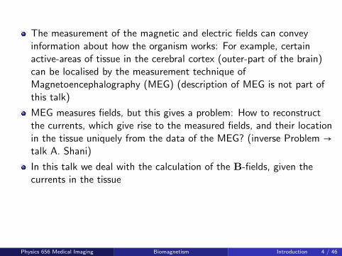
The measurement of the magnetic and electric fields can conveyinformation about how the organism works: For example, certainactive-areas of tissue in the cerebral cortex (outer-part of the brain)can be localised by the measurement technique ofMagnetoencephalography (MEG) (description of MEG is not part ofthis talk)

MEG measures fields, but this gives a problem: How to reconstructthe currents, which give rise to the measured fields, and their locationin the tissue uniquely from the data of the MEG? (inverse Problem →talk A. Shani)

In this talk we deal with the calculation of the B-fields, given thecurrents in the tissue


Magnetic Fields in the Human Body

Occurrences of magnetic fields

Magnetic constituents in the body (e.g. contaminants in the lung)

Magnetic moments of molecules

Ion currents in tissue

The magnetic fields, emitted bythe human body, range approxi-mately from nano- to femto-Tesla

Values of table taken from Hamalainen et al, RevModPhys,1993 and S.J. Williamson, L. Kaufman, Journal of Magnetismand Magnetic Materials, 1981

contaminants in the lung ∼ 1 nTheart-muscle ∼ 50 pTion currents in the eyes ∼ 10 pTbrain activity fT-pToptical brain stimulus ∼ 20 fTthermic magnetic noise(created by the thermicmotion of atoms)

∼ 1 fT


Currents

E- and B-fields are produced by currents. We introduce two types ofcurrents:

Primary current ji

Current-flow in active tissue (in intracellular-region also called ’impressedcurrent’, because ji gets ’impressed’ by biological activity)

Return current jV

Is evoked by the primary current: It ’neutralises’ the primary current bytransporting back the charge, which builds up through the primary current(also called ’volume current’, because it transports back the charge throughthe surrounding volume (tissue), in which the primary current is embedded)


Exact locations of the ’real’ currents are not known → primary currentand return current serve as theoretical models, representing the ’real’currents in the tissue

In our calculations, the total current is represented by the sum ofprimary current and return current


1 Introduction

2 Physiology



5 Approximations

6 Summary

7 References

Ion Mechanism in a Cell

Cells are surrounded by a membrane, dividing the space intointracellular- and extracellular-space

Ion-pump mechanism: Receptor molecules pump selected ions againstconcentration gradient of intra- and extracellular-space (e.g.Na+-K+-pump: 3 Na+ out, 2 K+ into the cell). Details of this or otherpump-mechanism are not discussed in this talk

According to the concentration gradient we get a potential differenceVin − Vext across the cell membrane → for an equilibrium state,currents (for each type of ion) must be balanced

Equilibrium: Concentration of certain ion-type Cion determined bythermodynamics (Boltzmann-distribution)

Cion ∼ exp(− ∣e∣Vion

kBT)⇒ Vion,in − Vion,ext =

kBT

∣e∣ln(

Cion,ext

Cion,in)

Physics 656 Medical Imaging Biomagnetism Physiology 9 / 46

Ion MechanismGoldman’s Equation

Vion,in − Vion,ext

K+ −89 mVCl− −48 mVNa+ 52 mV

(Values of the table taken from S.J. Williamson, L. Kaufman,Journal of Magnetism and Magnetic Materials, 1981)

Take K+, Cl−, Na+ for the totalmembrane-potential Vsimultaneously into account(Goldman’s equation):

V = kBT∣e∣

ln(P (K+)Cext,K+ + P (Na+)Cext,Na+ + P (Cl−)Cin,Cl−

P (K+)Cin,K+ + P (Na+)Cin,Na+ + P (Cl−)Cext,Cl−)

with P (ion) = permeability of the membrane with respect to that type ofion

This yields with typical values for humans and animals: V ≈ −70 mV

(Value taken from Hamalainen et al, RevModPhys, 1993)


Example: Pyramidal Neurons

(picture taken from Hamalainen et al, RevModPhys,1993)

structure

soma Cell-body (processessignals)

dendrites Thread-like endings(receive stimuli fromother cells)

axon Long fibre (carriesnerve impulses)

synapses Connections to otherneurons (releaseneurotransmitter foraction potential (→explained on the nextslide))


Action Potential (Pyramidal Neuron)

Action potential is an electric pulse, which travels from the axon-hill at thecell body along the axon to other neurons or cells

Action potentials are triggered by excitatory synaptic inputs. These areincreasing the membrane potential

Triggering mechanism

1 Synapses: Release neurotransmitters (some acid like glutamate)

2 Neurotransmitters bind to receptor molecules on cell membrane →change in membrane potential and permeability for a certain type ofions

3 Positive feedback loop: Rise of membrane potential opens ionchannels, this in return increases the membrane potential

4 ’Excitatory potential’ propagates exponentially damped to the cellbody → combined signal of several synapses must reach the axon-hill

5 Threshold ∼ −55 mV at the axon-hill triggers an action potential


Potential course (picture adopted from https://de.wikipedia.org/wiki/Aktionspotential

Threshold voltage

-70 Equilibrium voltage

Membrane potential / mV

0

Overshoot

Depolarisation

Repolarisation

Hyperpolarisation2 ms

-50


https://de.wikipedia.org/wiki/Aktionspotential

Depolarisation and Repolarisation

1 Positive-feedback evokes a rapid raise in the membrane potential →sodium and potassium channel becomes maximally opened

2 Sodium channel slowly closes, membrane permeability of sodiumbecomes lower relative to the permeability of potassium → membranevoltage falls

Overshoot and hyperpolarisation are inertial-phenomena, i.e. in case of theovershoot, more ions are flooding into the intracellular-space than wouldbe necessary for a zero membrane-voltage

The signal of the action potential propagates along the axon to otherneurons, to trigger again an action potential


Typical duration of an action potential of a neuron is 1 − 2 ms

Within the phases of repolarisation and hyperpolarisation it is notpossible to trigger an action potential anew (refractory period)

Amplitude of the action potential is independent of triggering-strength(’all-or-non’ principle), but not so the frequency → the stronger thesynaptic input, the higher the frequency (limited by refractory period)

Up to now it is unknown, how the entire process of an actionpotential conveys information


1 Introduction

2 Physiology



5 Approximations

6 Summary

7 References

Magnetic-Dipole

pair of poles

el. current (closed loop)

Magnetic-dipole can be represented by twomodels:

Pair of (contrary charged) poles

Closed loop (perfect circle) of electriccurrent

Important field components:

Direct field: Represented by those fieldline-pieces, which are orientated parallelto the magnetic moment m (B ⋅m > 0)

Return field: Represented by those fieldline-pieces, which are orientatedantiparallel to m (B ⋅m < 0)

(pictures taken from https://en.wikipedia.org/wiki/Magnetic_dipole)

Physics 656 Medical Imaging Biomagnetism Creation of the Fields 17 / 46

https://en.wikipedia.org/wiki/Magnetic_dipole)

Magnetic fields in organic systems are often very complicated close to thetissue. But in most cases the fields are measured outside of the body,

where the far-field approximation is sufficient. . .


Far-Field Approximation for the Vector-Potential A

For a magnetic-dipole, the vector potential A(r) can be written as

A(r) = µ0

4π∫

j(r′)∣r − r′∣

dr′

Taylor-expansion of 1/∣r− r′∣ yields so called multipole-expansion for A(r):

1

∣r − r′∣=

∞

∑n=0

1

n!(r′ ⋅ ∇r)n

1

∣r − r∣∣r=0

≈ 1

∣r∣+ 1

∣r∣3(r ⋅ r′) + 1

2∣r∣5(3(r ⋅ r′)2 − ∣r∣2∣r′∣2) + . . .

⇒A(r) ≈ µ0

4π∫ dr′ j(r′)( 1

∣r∣+ 1

∣r∣3(r ⋅ r′) +O ( 1

∣r∣5))

= µ0

4π∣r∣2 ∫dr′ j(r′)(er ⋅ r′)


Side Remark: Why No Magnetic Monopoles?

Define vector field (vanishing at infinity) Vk = r′kj(r′), k = 1,2,3

∇(Vk(r′)) = ∇(r′kj(r′))

=3

∑l=1

∂

∂r′l(r′kjl(r

′))

=3

∑l=1

[δkljl(r′) + r′k∂

∂rljl(r′)]

= jk(r′) + r′k∇j(r′)

Continuity equation (∂ρ/∂t +∇j(r′) = 0) for static charge-distribution:

∇j(r′) = 0

∫Ω=R3

dr′ jk(r′) = ∫Ωdr′∇(Vk(r′)) = ∮

∂ΩVk(r′)dS′ = 0


Impressed & Volume Current (ji & jV )

Impressed current ji

Arise from biological activity, especially from diffusion of ions

Establishes imbalance in Cion → evokes return current

Volume current jV

Is evoked by ji, prevents ionizing of the surrounding tissue

Is dictated by distribution of conductivity σ and E, where E arisesfrom the charge-transport of ji

Follows Ohm’s law jV = σ(r) ⋅E(r)

For jV we need to know σ, but σ is unknown → hint: Fromanimal-experiments, it is known, that σ is likely to be highly anisotropic

Total current → j = ji + jV


ji and jV can be combined to establish a ’current-dipole’. . .


Current-Dipole Q

Movement of localised charge over a short distance

Q = current ⋅ distance

Current-dipoles represent an unknowncurrent pattern in terms of ji and jV

Battery: Biochemical processes impressflow of charge (= ji) between ±-terminals

Back-flow (= jV ) prevents ionizing of tissue

jV = radially symmetric in- & out-flow.Pattern has same form as B of amagnetic-dipole

Orientation of the dipole in the direction ofimpressed current: Q∣∣ji

Also possible: Fixed charges as ±-pole(picture taken from S.J. Williamson and L. Kaufman, Journal of Magnetism andMagnetic Materials, 1981)


1 Introduction

2 Physiology



5 Approximations

6 Summary

7 References

Quasi-Static Limit

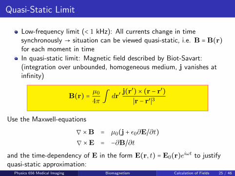
Low-frequency limit (< 1 kHz): All currents change in timesynchronously → situation can be viewed quasi-static, i.e. B = B(r)for each moment in time

In quasi-static limit: Magnetic field described by Biot-Savart:(integration over unbounded, homogeneous medium, j vanishes atinfinity)

B(r) = µ0

4π∫ dr′

j(r′) × (r − r′)∣r − r′∣3

Use the Maxwell-equations

∇×B = µ0(j + ε0∂E/∂t)∇×E = −∂B/∂t

and the time-dependency of E in the form E(r, t) = E0(r)eiωt to justifyquasi-static approximation:

Physics 656 Medical Imaging Biomagnetism Calculation of Fields 25 / 46

Side remark: Why is Quasi-Static Approximation Justified?

Insert j = σE + ∂P/∂t and P = (ε − ε0)E into

∇×B = µ0(j + ε0∂E/∂t)

⇒ ∇×B = µ0 (σE + ε∂E/∂t)

Constraint: Temporal part ε∂E/∂t must be smaller than σEwith E = E0(r)eiωt and ω = 2πf

⇒ ∣ε∂E/∂t∣ ≪ ∣σE∣⇔ ωε/σ ≪ 1

with f ∼ 100 Hz, σ = 0.3 Ω−1m−1, ε = 105ε0 → ωε/σ = 2 ⋅ 10−3 ≪ 1

∇×E = −∂B∂t⇔ ∇×∇×E = −µ0

∂

∂t(σ + iωε)E = −iωµ0σ(1 + ıωε/σ)E

Spatial changes of solution ∼ ∣ωµ0σ(1 + iωε/σ)∣−1/2 ≈ 65 m


Integral Formulas for V and B

B(r) = µ0

4π∫

j(r′) ×R

R3dr′ R = r − r′

Rewrite integrand with (∇ = Nabla-operator with respect to r, ∇′ =Nabla-operator with respect to r′)

R/R3 = −∇(1/R) = ∇′(1/R)

j ×∇′(1/R) = (∇′ × j)/R −∇′ × (j/R)

B(r) = µ0

4π

⎡⎢⎢⎢⎢⎢⎢⎢⎢⎣

∫∇′ × j(r′)

Rdr′ − ∫ ∇′ × ( j(r

′)R

)dr′

´¹¹¹¹¹¹¹¹¹¹¹¹¹¹¹¹¹¹¹¹¹¹¹¹¹¹¹¹¹¹¹¹¹¹¹¹¹¹¹¹¹¹¹¹¹¹¹¹¹¹¹¹¹¹¸¹¹¹¹¹¹¹¹¹¹¹¹¹¹¹¹¹¹¹¹¹¹¹¹¹¹¹¹¹¹¹¹¹¹¹¹¹¹¹¹¹¹¹¹¹¹¹¹¹¹¹¹¹¹¶Stokes→0

⎤⎥⎥⎥⎥⎥⎥⎥⎥⎦

= µ0

4π∫

∇′ × j(r′)R

dr′


Because ∇×E = −∂B/∂t ≈ 0⇒ E = −∇V ⇒ j = ji +Eσ = ji − σ∇VUse

∇′ × j = ∇× ji −∇ × σ∇V = ∇× ji −∇σ ×∇V = ∇× ji +∇ × (V∇σ)

B(r) = µ0

4π∫

∇′ × (ji(r′) + V∇′σ)R

dr′

= µ0

4π∫ (ji(r′) + V∇′σ) × R

R3dr′

We still need an eq.to determine V !

Use in quasi-static approximation:

∇ ⋅ [∇×B]´¹¹¹¹¹¹¹¹¹¹¹¹¹¹¹¹¹¹¹¹¹¹¹¸¹¹¹¹¹¹¹¹¹¹¹¹¹¹¹¹¹¹¹¹¹¹¹¶

=0

= µ0∇ ⋅ (j − ε0 ∂E/∂t´¹¹¹¹¹¸¹¹¹¹¹¶≈0

)⇔ ∇j = 0

∇ ⋅ (σ∇V ) = ∇ ⋅ ji Choose proper boundary conditions,solve for V and plug into eq. for B


1 Introduction

2 Physiology



5 Approximations

6 Summary

7 References

Piece-Wise Homogeneous Conductor

Gi: Area- or volume-partof the conductor

σi: Conductivity of thetissue in Gi (constant inGi)

Sij :Boundary-line/-surface,separating Gi from Gj

nij : Normal-vector ofSij , pointing(conventionally) from Gito Gj

Piece-wise homogeneous conductor

(picture taken from Hamalainen et al, RevModPhys, 1993)

Physics 656 Medical Imaging Biomagnetism Approximations 30 / 46

Equation for B in Case of a Piece-wise HomogeneousConductor

∇′σ only non-zero at boundaries. Use (G = ∪iGi) and j = ji − σ∇V

B(r) = µ0

4π∫G

j(r′) ×R

R3dr′ = B0(r) −

µ0

4π∑i

σi∫Gi

∇′V × R

R3dr′

with

B0(r) =µ0

4π∫Gji × R

R3dr′

Let’s rewrite the second term: Take a look at the vector identities:

∇× [(1/R)∇V ] = [∇(1/R)] ×∇V +

:0

(1/R) [∇×∇V ]0 = ∇×∇(V /R) = ∇× [(1/R)∇V + V∇(1/R)]

= ∇(1/R) ×∇V +∇ × V∇(1/R)

Therefore∇V ×∇(1/R) = ∇× V∇(1/R)


With this we get

∫Gi

∇′V × R

R3dr′ = ∫

Gi

∇′V ×∇′(1/R)dr′ = ∫Gi

∇′ × V∇′(1/R)dr′

Use the vector analysis relationship ∫G∇× adr = − ∫∂G a × dS (see D. B.Geselowitz, IEEE Transactions on Magnetics, Vol. Mag-6,No 2, 1970):

∫Gi

∇′ × V∇′(1/R)dr′ = −∫∂Gi

V∇′(1/R) × dSi

The integral is now taken over boundaries of neighbouring Gi,Gj (dSi = −dSj on∂Gi ∩ ∂Gj)

∑i

σi ∫∂Gi

(. . .)dSi = . . . + σi ∫∂Gi

(. . .)dSi + . . . + σj ∫∂Gj

(. . .)dSj + . . .

= . . . + (σi − σj)∫Sij=∂Gi∩∂Gj

(. . .)dSij + . . .

= ∑<i,j>

(σi − σj)∫Sij

(. . .)dSij + ext.boundary

⇒ B(r) = B0(r) + µ0

4π ∑ij(σi − σj) ∫SijV (r′) R

R3 × dS′ij


Integral Equation for V

For B(r), we need again an expression for V . Use Green’s second identity

∫G(φ∇2ψ − ψ∇2φ)dr = ∫

S=∂G(φ∇ψ − ψ∇φ)dS

which relates a volume-integral of an integrand involving two differentiablescalar-functions ψ and φ and the ∇-operator to an integral over theboundary-surface if we insert ψ = 1/R, R = ∣r − r′∣ and φ = V , we canderive an integral-equation for V in order to determine V .

This adopted to our problem reads:

∑i

σi∫Gi

[ 1

R∇′2V − V∇′2 1

R] dr′ = ∑

ij∫Sij

[σi [1

R∇′Vi − Vi∇′ 1

R]

−σj [1

R∇′Vj − Vj∇′ 1

R]] ⋅ dS′ij


Use continuity of current at boundaries (remember: jV = σ ⋅E = −σ ⋅ ∇V ):

Vi(dS′ij) = Vj(dS′ij)σi∇′Vi ⋅ dS′ij = σj∇′Vj ⋅ dS′ij

as well as the Laplace-equation

∇′2(1/R) = −4πδ(3)(R)

which in general can be stated in terms of Green’s function G(a,b)

∇2G(a,b) = δ(3)(a − b)

with the solution

G(a,b) = −1

4π∣a − b∣Physics 656 Medical Imaging Biomagnetism Approximations 34 / 46

∑i

σi∫Gi

V∇′2 1

Rdr′ = 4πσ0V (R = 0)

Therefore:

(∑i

σi∫Gi

1

R∇′2V dr′)+4πσ0V (R = 0) = −∑

ij

(σi−σj)∫Sij

V∇′(1/R)⋅dS′ij


In quasi-static approximation:

∇ ⋅ j = 0⇔ ∇ ⋅ σ∇V = ∇ ⋅ ji

we get

4πσ0V (R = 0) = −∑i∫Gi

1

R∇′ ⋅ ji dr′ −∑

ij

(σi − σj)∫Sij

(V∇′ 1

R) ⋅ dS′ij

Rewrite the first term:

∑i∫Gi

∇′ ⋅ ( ji

R) dr′ =∑

ij∫Sij

1

Rji ⋅ dSij = ∫

G(ji ⋅ ∇ 1

R+ 1

R∇ ⋅ ji) dr′

Since ji vanishes on Sij , we get

∫G

1

R∇ ⋅ ji dr′ = −∫

Gji ⋅ ∇ 1

Rdr′


Therefore, we obtain

4πσ0V (R = 0) = ∫Gji ⋅ ∇ 1

Rdr′ −∑

ij

(σi − σj)∫Sij

(V∇′ 1

R) ⋅ dS′ij

= ∫Gji ⋅ R

R3dr′

´¹¹¹¹¹¹¹¹¹¹¹¹¹¹¹¹¹¹¹¹¹¹¹¹¹¹¹¹¹¹¹¸¹¹¹¹¹¹¹¹¹¹¹¹¹¹¹¹¹¹¹¹¹¹¹¹¹¹¹¹¹¹¹¶4πσ0V0(r)

−∑ij

(σi − σj)∫Sij

VR

R3⋅ dS′ij

V (R = ∣r − r′∣ = 0) = V0(r) −1

4πσ0∑ij

(σi − σj)∫Sij

VR

R3⋅ dS′ij

Integral equation for V (R = 0) → determines V in the integration-area,which is exactly what we need in order to calculate B! B


Spherically Symmetric Conductor

The axons of pyramidal neurons in thecerebral cortex tissue are approximatelyparallel to each other and perpendicular tothe scull-surface

(picture taken from https://en.wikipedia.org/wiki/Neuron)

→ approximate head by anhomogeneous sphericallysymmetric conductor →currents in the axonsrepresented by

radial-current pattern

Approximation not realistic,but greatly simplifies solutionfor B:


https://en.wikipedia.org/wiki/Neuron

B for a Spherically Symmetric Conductor

B(r) = B0(r) +µ0

4π∑ij

(σi − σj)∫Sij

V (r′) RR3

× dS′ij

´¹¹¹¹¹¹¹¹¹¹¹¹¹¹¹¹¹¹¹¹¹¹¹¹¹¹¹¹¹¹¹¹¹¹¹¹¹¹¹¹¹¹¹¹¹¹¹¹¹¹¹¹¹¹¹¹¹¹¹¹¹¹¹¹¹¹¹¹¹¹¹¹¹¹¹¹¹¹¹¹¹¹¹¹¹¹¹¹¹¹¹¹¹¹¹¹¹¹¹¹¹¹¹¹¹¹¹¹¹¹¹¹¹¹¹¹¸¹¹¹¹¹¹¹¹¹¹¹¹¹¹¹¹¹¹¹¹¹¹¹¹¹¹¹¹¹¹¹¹¹¹¹¹¹¹¹¹¹¹¹¹¹¹¹¹¹¹¹¹¹¹¹¹¹¹¹¹¹¹¹¹¹¹¹¹¹¹¹¹¹¹¹¹¹¹¹¹¹¹¹¹¹¹¹¹¹¹¹¹¹¹¹¹¹¹¹¹¹¹¹¹¹¹¹¹¹¹¹¹¹¹¹¹¶=0

⇒ contribution of jV to the radial field component

Br = B(r) ⋅ er = B(r) ⋅ r/∣r∣

vanishes, since (dS = n(r) ⋅ dS, i.e. normal-vector of dS )

(r − r′) × n(r′) ⋅ er = (r − r′) × r′

∣r′∣⋅ r∣r∣

= 0

→ calculate Br with ji(r′) =Qδ(3)(r′ − rQ) (rQ = location of thecurrent-dipole Q)

Br =µ0

4π∫

ji(r′) ×R

R3dr′ = µ0

4π

Q × rQ ⋅ er∣r − rQ∣3


1 Introduction

2 Physiology



5 Approximations

6 Summary

7 References

Summary

Biomagnetism: Magnetic fields (and also electric fields) arise fromcurrents, impressed by biological activity

Primary- & return-current: Represent real current pattern. Totalcurrent: j = ji + jV

Current-dipole: Represented by a battery. ji connects ±-terminals,jV symbolizes radial symmetric inflow pattern (alternatively: twocharges, which evoke the same field pattern as a magnetic dipole)

Far-field approximation: B(r) can be approximated by the dipolemoment (multipole expansion)

Quasi-static limit: Basis for calculation of fields

all currents in tissue change synchronouslyfor each moment in time, neglect time-dependent parts inMaxwell-equationsB described by Biot-Savart

Physics 656 Medical Imaging Biomagnetism Summary 41 / 46

General conductorApplying quasi-static limit & concept of ji and jV to Biot-Savart → get anequation for B(r) and a differential equation for V :

B(r) = µ0

4π∫ (ji(r′) + V∇′σ) × R

R3dr′

∇ ⋅ (σ∇V ) = ∇ ⋅ ji


Piece-Wise Homogeneous conductorSplit G into Gi with σi = const. Use vector identities and Stoke’s Theorem:

B(r) = B0(r) +µ0

4π∑ij

(σi − σj)∫Sij

V (r′) RR3

× dS′ij

For V , we use a trick by applying Green’s second identity and exploit thecontinuity of the currents at boundaries:

V (R = ∣r − r′∣ = 0) = σ0V0(r) −1

4πσ0∑ij

(σi − σj)∫Sij

VR

R3⋅ dS′ij


Spherically symmetric conductor

jV does not contribute to B(r) → Choosing the limit of a point-likecurrent (ji =Qδ(3)(r − rQ), rQ = position of the current-dipole), B(r)simplifies to

B(r) = µ0

4π∫

ji(r′) ×R

R3dr′ = µ0

4π

Q × rQ ⋅ er∣r − rQ∣3


1 Introduction

2 Physiology



5 Approximations

6 Summary

7 References

References

Hamalainen et alMagnetoencephalography - theory, instrumentation, and applicationsto noninvasive studies of the workin human brainRev. Mod. Phys., 1993

Davi B. GeselowitzOn Bioelectric Potentials in an Inhomogeneous Volume ConductorBioPhys Journal, 1967

David B. GeselowitzOn the Magnetic Field Generated Outside an Inhomogeneous VolumeConductor by Internal Current SourcesIEEE Transactions on Magnetics, Vol. Mag-6,No 2, 1970

S.J. Williamson, L. KaufmanBiomagnetismJournal of Magnetism and Magnetic Materials 22, 129-201, 1981

Physics 656 Medical Imaging Biomagnetism References 46 / 46

basics of biomagnetism -...

Documents