Basic probability theory

Sharon GoldwaterInstitute for Language, Cognition and Computation

School of Informatics, University of Edinburgh

DRAFT Version 0.95: 25 Sep 2016. Do not redistribute without permission.

Contents

1 Purpose of this tutorial and how to use it 2

2 Events and Probabilities 22.1 What is probability and why do we care? . . . . . . . . . . . . . . . . . . . 22.2 Sample spaces and events . . . . . . . . . . . . . . . . . . . . . . . . . . . 42.3 The probability of an event . . . . . . . . . . . . . . . . . . . . . . . . . . 52.4 Probability distributions . . . . . . . . . . . . . . . . . . . . . . . . . . . . 62.5 Exercises . . . . . . . . . . . . . . . . . . . . . . . . . . . . . . . . . . . 7

3 Combining events 103.1 Event complement and union . . . . . . . . . . . . . . . . . . . . . . . . . 103.2 Joint probabilities and the law of total probability . . . . . . . . . . . . . . 113.3 Exercises . . . . . . . . . . . . . . . . . . . . . . . . . . . . . . . . . . . 12

4 Conditional probabilities, independence, and Bayes’ Rule 134.1 Definition of conditional probability . . . . . . . . . . . . . . . . . . . . . 134.2 The product rule and chain rule . . . . . . . . . . . . . . . . . . . . . . . . 134.3 Conditional probability distributions . . . . . . . . . . . . . . . . . . . . . 144.4 Conditional and joint probability tables . . . . . . . . . . . . . . . . . . . 154.5 Independent events . . . . . . . . . . . . . . . . . . . . . . . . . . . . . . 164.6 Bayes’ Rule . . . . . . . . . . . . . . . . . . . . . . . . . . . . . . . . . . 174.7 Exercises . . . . . . . . . . . . . . . . . . . . . . . . . . . . . . . . . . . 19

5 Random variables and discrete distributions 215.1 Definition of a random variable . . . . . . . . . . . . . . . . . . . . . . . . 215.2 The geometric distribution . . . . . . . . . . . . . . . . . . . . . . . . . . 225.3 Other discrete distributions . . . . . . . . . . . . . . . . . . . . . . . . . . 235.4 Restating the probability rules using random variables . . . . . . . . . . . . 245.5 Working with more than two variables . . . . . . . . . . . . . . . . . . . . 255.6 Exercises . . . . . . . . . . . . . . . . . . . . . . . . . . . . . . . . . . . 27

6 Expectation and variance 286.1 Definitions . . . . . . . . . . . . . . . . . . . . . . . . . . . . . . . . . . . 286.2 Exercises . . . . . . . . . . . . . . . . . . . . . . . . . . . . . . . . . . . 30

7 Continuous random variables 30

8 A note about estimating probabilities from data 32

9 Solutions to selected exercises 33

1

1 Purpose of this tutorial and how to use it

This tutorial is written as an introduction to probability theory aimed at upper-level under-graduates or MSc students who have little or no background in this area of mathematicsbut who want to take courses on (or even just read up on) computational linguistics, naturallanguage processing, computational cognitive science, or introductory machine learning.Many textbooks in these areas (even introductory ones such as Jurafsky & Martin’s Speechand Language Processing or Witten et al’s Data Mining assume either implicitly or explicitlythat students are already familiar with basic probability theory. Yet many students withbackgrounds in linguistics, psychology, or other social sciences (and even some computerscience students) have very little exposure to probability theory.

I have taught students like these in courses on NLP and computational cognitive science,I have tried to find existing materials, preferably free ones, to refer students to. Howeverall the materials I’ve seen are either too extensive and formal (mainly textbooks aimed atstudents of mathematics and related subjects) or too basic and incomplete (mainly onlinetutorials aimed at students learning statistics for social science, which have a very differentfocus and don’t cover all the material needed by my target group). Some online videos (e.g.,from Khan Academy) cover relevant material, but don’t come with written notes containingdefinitions and equations for reference.

So, I ultimately decided to write my own tutorial. This tutorial is a work in progress. Ihave tried to include the most critical topics and to provide a lot of examples and exercises(although the exercises are not finished for all sections yet). Students from non-mathematicalbackgrounds sometimes have trouble with formal notation, so I have tried to explain thenotation carefully and to be consistent in my own use of notation. However, I’ve also tried topoint out variations of the notation that other authors may use, in the hope that when you arereading other materials you will have an easier time relating them back to this tutorial anddeciphering the notation even if it isn’t exactly the same as what I use here.

Don’t expect that you can simply read through this tutorial once and understand every-thing. Reading mathematics is not like reading a novel: you will need to work at it. You mayneed to flip back and forth to remind yourself of definitions and equations, and you shouldask yourself as you are reading through each example: does this make sense to me? If youfind your attention wandering, consider taking a break. You won’t learn much if you are justskimming without thinking.

Finally, I strongly recommend that you actually do the exercises. Like any area ofmathematics, the only way to really understand probability theory and be able to solveproblems is to practice! I have included solutions for some of the exercises at the end of thetutorial, but you should only look at them after you have worked out your own solution. It isvery easy to trick yourself into thinking that you understand something if you look at thesolution before working it out fully.

I’ve done my best to proofread this tutorial, but if you do find any errors, please let meknow.

2 Events and Probabilities

2.1 What is probability and why do we care?

Probability theory is a branch of mathematics that allows us to reason about events that areinherently random. However, it can be surprisingly difficult to define what “probability” iswith respect to the real world, without self-referential definitions. For example, you mighttry to define probability as follows:

Suppose I perform an action that can produce one of n different possible random OUT-COMES, each of which is equally likely. (For example, I flip a fair coin to produce one of OUTCOMES

two outcomes: heads or tails. Or, I pick one of the 52 different cards from a deck of playing

2

cards at random.) Then, the probability of each of those outcomes is 1/n. (So, 1/2 for headsor tails; 1/52 for each of the possible cards.)

The problem with this definition is that it says each random outcome is “equally likely”.But what does that mean, if we cannot define it in terms of the probability of differentoutcomes? Nevertheless, the above definition may begin to give you some intuition aboutprobability.

Another way to think about probability is in terms of repeatable experiments. By “ex-periment”, I mean a STATISTICAL EXPERIMENT. A statistical experiment is an action or STATISTICAL

EXPERIMENToccurrence that can have multiple different outcomes, all of which can be specified in ad-vance, but where the particular outcome that will occur cannot be specified in advancebecause it depends on random chance. Flipping a coin or choosing a card from a deck atrandom are both statistical experiments. They are also repeatable experiments, because wecan perform them multiple times (flip the same coin many times in a row, or return ouroriginal card to the deck and choose another card at random).

So, if we have a repeatable experiment, then one way to think about probability is asfollows. Suppose we repeat the experiment an infinite number of times. The probability of aparticular outcome is the proportion of times we get that outcome out of our infinite numberof trials. For example, if we flip the fair coin an infinite number of times, we should expectto get a head 1/2 of those times.

This definition is not self-referential, but it also has problems. What if our experimentis not repeatable? For example, what if we want to know the probability that it will raintomorrow? There is certainly some probability associated with that outcome, but no way todetermine it (or even approximate it) by a repeatable experiment. So, a third way to thinkabout probability is as a way of talking about and mathematically working with degrees ofbelief. If I say “the probability of rain tomorrow is 75%”, that is a way of expressing the factthat my belief in rain tomorrow is fairly strong, and I would be somewhat surprised if it didnot rain. On the other hand, if I say “the probability of rain tomorrow is 2%”, I have a verystrong belief that it will not rain, and I would be very surprised if it did.

Whichever way you want to think about probabilities, they turn out to be extraordinarilyuseful in many areas of cognitive science and artificial intelligence. Broadly speaking,probabilities can be used for two types of problems:

a) Generation/prediction. Reasoning from causes to effects:1 Given a known set ofcauses and knowledge about how they interact, what are likely/unlikely outcomes? Forexample, we could set up a probabilistic system that generates sequences of charactersas follows: Roll a fair 6-sided die. If the result is 1 or 2, print an a. Otherwise, printa b. This isn’t a terribly interesting generative process, but we could use probabilitytheory to determine things like: how likely are we to get an a for the next character? Ifwe generate a sequence of 10 characters, how likely are we to get at least four a’s?And so forth.

Much of the early work developing probability theory was motivated by answeringquestions like these in order to be able to predict how often certain events would occurin gambling. However, even if we are not interested in gambling, it’s often useful to beable to make these kinds of predictions.

b) Inference. Reasoning from effects to causes: Given knowledge about possible causesand how they interact, as well as some observed outcomes, which causes arelikely/unlikely? Here are some examples:

• observe many outcomes of a coin flip⇒ determine if coin is fair.

1In machine learning, causes are often referred to as hidden or latent variables, and effects as observedvariables. This terminology is more general and often more appropriate, since it doesn’t imply causation in everycase.

3

• observe features of an image⇒ determine if it is a cat or dog.

• observe patient’s symptoms⇒ determine disease.

• observe words in sentence⇒ infer syntactic parse.

In everyday reasoning, we often do both inference and prediction. For example, we mightfirst infer the category of an object we see (cat or dog?) in order to predict its future behavior(purr or bark?). In the following sections, we’ll work through some of the mathematicalbackground we need in order to formalize the problems of generation and inference, andthen we’ll show some examples of how to use these ideas.

2.2 Sample spaces and events

Let’s start with some basic definitions:

• The SAMPLE SPACE of a statistical experiment is the set of all possible outcomes (also SAMPLE SPACE

known as SAMPLE POINTS). SAMPLE POINTS

• An EVENT is a subset of the sample space. EVENT

Example 2.2.1. Imagine I flip a coin, with two possible outcomes: heads (H) or tails (T).What is the sample space for this experiment? What about for three flips in a row?

Solution: For the first experiment (flip a coin once), the sample space is just{H,T}. For the second experiment (flip a coin three times), the sample space is{HHH,HHT,HTH,HTT,THH,THT,TTH,TTT}. Order matters: HHT is a different outcome thanHTH.

Example 2.2.2. For the experiment where I flip a coin three times in a row, consider theevent that I get exactly one T. Which outcomes are in this event?

Solution: The subset of the sample space that contains all outcomes with exactly one T is{HHT,HTH,THH}.

Example 2.2.3. Suppose I have two bowls, each containing 100 balls numbered 1 through100. I pick a ball at random from each bowl and look at the numbers on them. How manyelements are in the sample space for this experiment?

Solution: Using basic principles of counting (see the Sets and Counting tutorial), since thenumber of possible outcomes for the second experiment doesn’t depend on the outcome ofthe first experiment, the total number of possible outcomes is 1002, or 10,000.

Example 2.2.4. Which set of outcomes defines the event that the two balls add up to 200?

Solution: There is only one outcome in this event, namely {(100,100)}.

Example 2.2.5. Let E be the event that the two balls add up to 201. Which outcomes areelements of E?

Solution: This is no outcome in which the balls can add up to 201, so E = /0.

The last example illustrates the idea of an IMPOSSIBLE EVENT, an event which contains IMPOSSIBLE EVENT

no outcomes. In contrast, a CERTAIN EVENT is an event that contains all possible outcomes. CERTAIN EVENT

For example, in the experiment where I flip a coin three times, the event that we obtain atleast one H or one T is a certain event.2

2In real life, this event would not be certain, since there is some very small chance the coin might land onits edge, or fall down a hole and be lost, or be eaten by a cat before landing. However, in this case I definedthe possible outcomes at the outset as only H or T , so these real-life possibilities are not possibilities in myidealized experiment. Certain and impossible events are very rare in real life, but less rare in the idealized worldof mathematics.

4

2.3 The probability of an event

Now, let’s consider the probability of an event. By definition, an impossible event hasprobability zero, and a certain event has probability one. The more interesting cases areevents that are neither impossible nor certain. For the moment, let’s assume that all outcomesin the sample space S are equally likely. If that is the case, then the probability of an eventE, which we write as P(E), is simply the number of outcomes in E divided by number ofoutcomes in S:

P(E) =|E||S|

if all outcomes in S are equally likely (1)

That is, the probability of an event is the proportion of outcomes in the sample space that arealso outcomes in that event.

Example 2.3.1. Imagine I flip a fair coin, with two possible outcomes: heads (H) or tails (T).What is the probability that I get exactly one T if I flip the coin once? What if I flip it threetimes?

Solution: First, note that I said it’s a fair coin. This is important, because it means that on anyone flip, each outcome is equally likely, so we can use (1) to determine the probabilities wecare about. We already determined the relevant events and sample spaces for each experimentin the previous section, so now we just need to divide those numbers. Specifically, if we onlyflip the coin once, then the event we care about (getting T) has one possible outcome, and thesample space has two possible outcomes, so the probability of getting T is 1/2. If we flip thecoin three times, there are three outcomes with exactly one T (see Example 2.2.2), and eightoutcomes altogether (see Example 2.2.1), so the probability of getting exactly one T is 3/8.

Example 2.3.2. Suppose I have two bowls, each containing 100 balls numbered 1 through100. I pick a ball at random from each bowl and look at the numbers on them. What is theprobability that the numbers add up to 200?

Solution: Again, we already computed that there is only one outcome in this event, and10,000 outcomes altogether, so the probability of this happening is only 1/10,000

Example 2.3.3. Let E be the event that the numbers on the balls in the previous exampleadd up to exactly 51. What is the probability of E?

Solution: We already know the size of the sample space, but we also need to determine thecardinality of E, i.e., the number of outcomes in this event. Consider what happens if thefirst ball is 1. For the balls to add up to 51, it must be the case that the second ball is 50.Similarly, if the first ball is 2, then the second must be 49. And so on: for each possible firstball between 1 and 50, there is exactly one second ball that will make the total equal 51. Sothe total number of outcomes adding up to 51 is the same as the number of ways the firstball can be between 1 and 50, which is to say, 50 ways. Therefore, the probability of E is50/10,000, or 0.5%.

Example 2.3.4. Suppose I choose a PIN containing exactly 4 digits, where each digit ischosen at random and is equally likely to be any of the 10 digits 0-9. What is the probabilitythat my PIN contains four different digits?

Solution: First, consider the sample space S: all possible four-digit PINs. Using our countingtechniques (see Sets and Counting), we can compute that the number of outcomes in thissample space is 104, or 10,000. Next, consider the event E of interest: the set of PINs withfour distinct digits. To compute the size of this set, note that there are 10 possibilities for thefirst digit. Once that digit is determined, there are only 9 possibilities for the second digit,because it must be different from the first one. Then, 8 possibilities for the third digit (whichmust be different to both of the first two), and 7 for the final digit. So, the total number of

5

PINs with four different digits is 10 ·9 ·8 ·7, or 5040. Therefore P(E) = 5040/10,000, orvery slightly more than 1/2.

Example 2.3.5. Suppose I have a bowl with 3 green balls (g), 2 blue balls (b), and 1 red ball(r). I draw a single ball at random from the bowl and report its color. What is the probabilityI got a blue ball?

Solution: The answer may already be obvious to you, but let’s make sure we know how to getthere using the tools of probability theory that we’ve seen so far. Notice that if we define theoutcomes in our sample space as {g,b,r}, they are not equally likely, so we cannot use Eq(1). In this problem, the equally likely outcomes are the outcomes of drawing each particularball, a sample space of size 6. The events of interest are still {g,b,r}, but now we can useEq (1), which tells us that P(b) = 2/6 = 1/3 because two out of the six balls (outcomes) areblue.

2.4 Probability distributions

Hopefully you have developed some intuition for probabilities at this point. Before goingfurther, we should formalize what makes a probability a probability, mathematically speaking.To do so, we first need to define MUTUALLY EXCLUSIVE (or DISJOINT) events. Two events MUTUALLY

EXCLUSIVEDISJOINT

are mutually exclusive iff (“iff” means “if and only if”) they contain no outcomes in common(i.e., both events cannot occur at the same time). For example, if I roll two dice, the events“get a total of 7” and “get a total of 8” are mutually exclusive. On the other hand, “get a totalof 7” and “get a 6 on one die” are not mutually exclusive, since both could occur on the sameroll.

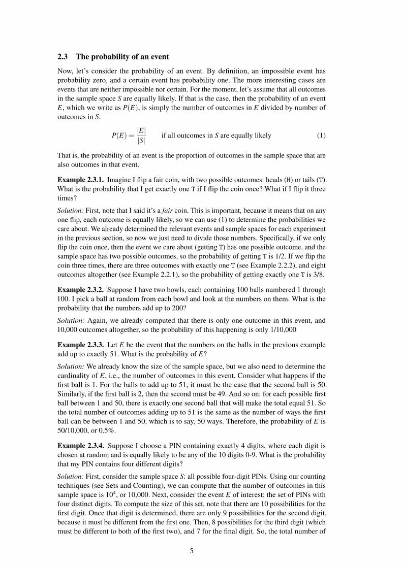
Now, suppose we have a set of n mutually exclusive events that together cover all possibleoutcomes in our sample space S. Such a set is called a PARTITION of the sample space, and PARTITION

is visualized in Figure 1. A simple example would be flipping a coin, where S = {H,T} andwe define n = 2 mutually exclusive events, E1 = {H} and E2 = {T}. Another example mightbe rolling two 6-sided dice, where the mutually exclusive events are getting a total of 2 or 3or 4 or . . . or 12 (in this case, n = 11 different events).

Figure 1: A partition of the sample space into four mutually exclusive events. The rectanglerepresents all the outcomes in the entire sample space, and each labelled region representsthe outcomes in that event.

We then assign a number, P(Ei), to each of the events Ei in the partition. If and only ifthe following two properties hold, then each P(Ei) can be considered a probability, and theset of values {P(E1) . . .P(En)} can be considered a PROBABILITY DISTRIBUTION. PROBABILITY

DISTRIBUTION

Property 1: 0≤ P(Ei)≤ 1

Property 2:n

∑i=1

P(Ei) = 1

6

That is, every probability must fall between 0 and 1 (inclusive), and the sum of theprobabilities of the mutually exclusive events that cover the the sample space must equal 1.

One way to think of a probability distribution is that altogether the sample space S hasone unit of PROBABILITY MASS, and this mass is divided up (distributed) in some way PROBABILITY MASS

between all the Ei. The amount of mass assigned to each Ei is what we call P(Ei). In ourcoin flipping example, the two events are equally likely, so the mass is divided evenly and weget P(E1) = P(E2) = 1/2. This is an example of a UNIFORM DISTRIBUTION, a distribution UNIFORM

DISTRIBUTIONwhere all events in a partition are equally likely. Another example of a uniform distributionis the distribution over the number we get when we roll a single fair die.

Since a probability distribution is defined as a function from events to values, it issometimes also called a PROBABILITY MASS FUNCTION: a function that allocates the PROBABILITY MASS

FUNCTIONprobability mass to the different events.3

Example 2.4.1. I have a jar with four different colored balls and I choose one at random. Isthe distribution over the color I get uniform or not?

Solution: If we assume that “choose one at random” means that each ball (and therefore eachcolor) is equally likely, then yes. However the phrase “at random” is ambiguous: technically,it just means there is some randomness involved, not necessarily that all outcomes are equallylikely. So, when working with probabilities, we usually try to be more specific. If we meanthat the distribution is uniform, then we should say that a ball is chosen UNIFORMLY AT

RANDOM. UNIFORMLY ATRANDOM

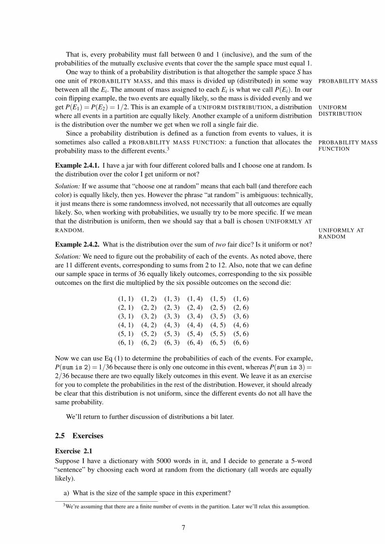
Example 2.4.2. What is the distribution over the sum of two fair dice? Is it uniform or not?

Solution: We need to figure out the probability of each of the events. As noted above, thereare 11 different events, corresponding to sums from 2 to 12. Also, note that we can defineour sample space in terms of 36 equally likely outcomes, corresponding to the six possibleoutcomes on the first die multiplied by the six possible outcomes on the second die:

(1, 1) (1, 2) (1, 3) (1, 4) (1, 5) (1, 6)(2, 1) (2, 2) (2, 3) (2, 4) (2, 5) (2, 6)(3, 1) (3, 2) (3, 3) (3, 4) (3, 5) (3, 6)(4, 1) (4, 2) (4, 3) (4, 4) (4, 5) (4, 6)(5, 1) (5, 2) (5, 3) (5, 4) (5, 5) (5, 6)(6, 1) (6, 2) (6, 3) (6, 4) (6, 5) (6, 6)

Now we can use Eq (1) to determine the probabilities of each of the events. For example,P(sum is 2) = 1/36 because there is only one outcome in this event, whereas P(sum is 3) =2/36 because there are two equally likely outcomes in this event. We leave it as an exercisefor you to complete the probabilities in the rest of the distribution. However, it should alreadybe clear that this distribution is not uniform, since the different events do not all have thesame probability.

We’ll return to further discussion of distributions a bit later.

2.5 Exercises

Exercise 2.1Suppose I have a dictionary with 5000 words in it, and I decide to generate a 5-word“sentence” by choosing each word at random from the dictionary (all words are equallylikely).

a) What is the size of the sample space in this experiment?

3We’re assuming that there are a finite number of events in the partition. Later we’ll relax this assumption.

7

b) If E is the event “my sentence starts with the word the”, how many outcomes are therein E?

c) What is P(E)?

d) Let A be the event “my sentence ends with the word the”. Are A and E mutuallyexclusive? If so, explain why. If not, give an example of an outcome that belongs toboth A and E.

Exercise 2.2Which of the following are possible probability distributions? For each distribution, statewhether it is uniform or not, and whether the distribution includes a certain or impossibleevent.Note: We are using a notation that assumes an ordering over events and just lists theprobabilities of those events as a vector in the appropriate order. For example, if we had twoevents, E1 and E2, with P(E1) = 1/3 and P(E2) = 2/3, we would write down this distributionas (1/3, 2/3).

a) (1.3, 2)

b) (0.2, 0.2, 0.2, 0.2)

c) (0.2, 0.2, 0.2, 0.2, -0.1, 0.3)

d) (0.2, 0.2, 0.2, 0.2, 0.2)

e) (0, 1, 0)

f) (0)

g) (1)

h) (-.5, -.5)

i) (1/2, 1/2)

j) (1/2, 1/4)

k) (1/8, 1/4, 5/8)

l) (3/16, 1/8, 7/16)

Exercise 2.3Write down the full distribution over the sum of two fair dice. That is, complete the examplewe started at the end of the last section (Example 2.4.2).

Exercise 2.4Suppose I have a bowl with 4 green balls (g), 2 blue balls (b), and 3 red balls (r). I draw asingle ball uniformly at random from the bowl and report its color. What is the probabilitydistribution over the different colors?

Exercise 2.5Suppose I have a bowl with 10 balls in it, all of which are either blue, red, or green. I draw asingle ball uniformly at random and report its color. The number of balls of each color issuch that the probability of getting a blue ball is 0.4 and the probability of getting a greenball is 0.3. What is the probability of getting a red ball? How many balls of each color arethere?

8

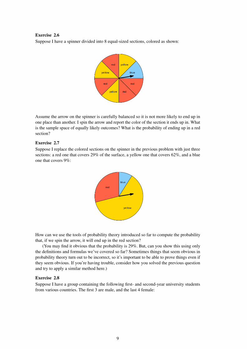
Exercise 2.6Suppose I have a spinner divided into 8 equal-sized sections, colored as shown:

Assume the arrow on the spinner is carefully balanced so it is not more likely to end up inone place than another. I spin the arrow and report the color of the section it ends up in. Whatis the sample space of equally likely outcomes? What is the probability of ending up in a redsection?

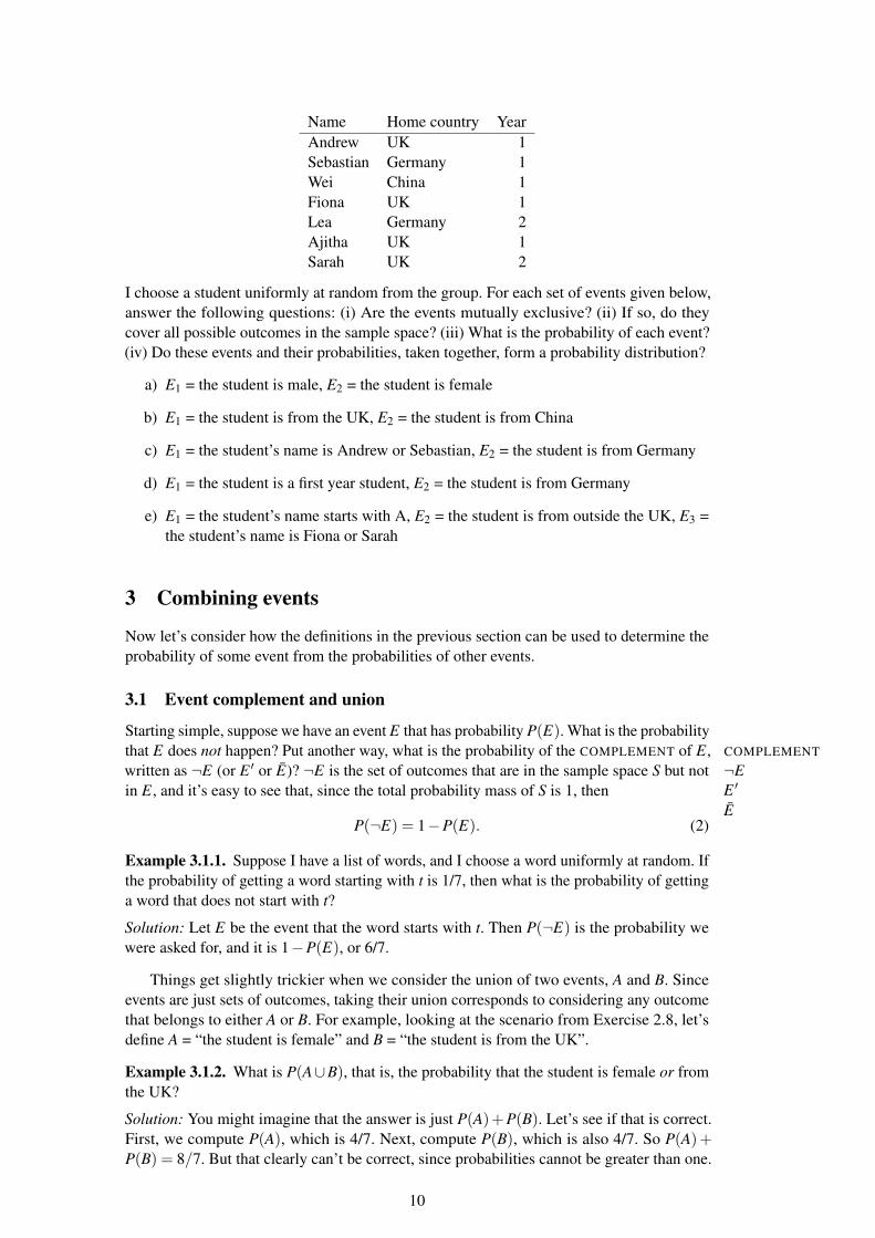
Exercise 2.7Suppose I replace the colored sections on the spinner in the previous problem with just threesections: a red one that covers 29% of the surface, a yellow one that covers 62%, and a blueone that covers 9%:

How can we use the tools of probability theory introduced so far to compute the probabilitythat, if we spin the arrow, it will end up in the red section?

(You may find it obvious that the probability is 29%. But, can you show this using onlythe definitions and formulas we’ve covered so far? Sometimes things that seem obvious inprobability theory turn out to be incorrect, so it’s important to be able to prove things even ifthey seem obvious. If you’re having trouble, consider how you solved the previous questionand try to apply a similar method here.)

Exercise 2.8Suppose I have a group containing the following first- and second-year university studentsfrom various countries. The first 3 are male, and the last 4 female:

9

Name Home country YearAndrew UK 1Sebastian Germany 1Wei China 1Fiona UK 1Lea Germany 2Ajitha UK 1Sarah UK 2

I choose a student uniformly at random from the group. For each set of events given below,answer the following questions: (i) Are the events mutually exclusive? (ii) If so, do theycover all possible outcomes in the sample space? (iii) What is the probability of each event?(iv) Do these events and their probabilities, taken together, form a probability distribution?

a) E1 = the student is male, E2 = the student is female

b) E1 = the student is from the UK, E2 = the student is from China

c) E1 = the student’s name is Andrew or Sebastian, E2 = the student is from Germany

d) E1 = the student is a first year student, E2 = the student is from Germany

e) E1 = the student’s name starts with A, E2 = the student is from outside the UK, E3 =the student’s name is Fiona or Sarah

3 Combining events

Now let’s consider how the definitions in the previous section can be used to determine theprobability of some event from the probabilities of other events.

3.1 Event complement and union

Starting simple, suppose we have an event E that has probability P(E). What is the probabilitythat E does not happen? Put another way, what is the probability of the COMPLEMENT of E, COMPLEMENT

written as ¬E (or E ′ or E)? ¬E is the set of outcomes that are in the sample space S but not ¬EE ′

Ein E, and it’s easy to see that, since the total probability mass of S is 1, then

P(¬E) = 1−P(E). (2)

Example 3.1.1. Suppose I have a list of words, and I choose a word uniformly at random. Ifthe probability of getting a word starting with t is 1/7, then what is the probability of gettinga word that does not start with t?

Solution: Let E be the event that the word starts with t. Then P(¬E) is the probability wewere asked for, and it is 1−P(E), or 6/7.

Things get slightly trickier when we consider the union of two events, A and B. Sinceevents are just sets of outcomes, taking their union corresponds to considering any outcomethat belongs to either A or B. For example, looking at the scenario from Exercise 2.8, let’sdefine A = “the student is female” and B = “the student is from the UK”.

Example 3.1.2. What is P(A∪B), that is, the probability that the student is female or fromthe UK?

Solution: You might imagine that the answer is just P(A)+P(B). Let’s see if that is correct.First, we compute P(A), which is 4/7. Next, compute P(B), which is also 4/7. So P(A)+P(B) = 8/7. But that clearly can’t be correct, since probabilities cannot be greater than one.

10

So, let’s instead consider which outcomes are actually in the set A∪B. They are: {Fiona,Lea, Ajitha, Sarah, Andrew}. Since this set has five elements, we know from Eq (1) thatP(A∪B) must be 5/7.

So what went wrong when we computed P(A) + P(B)? Notice that there are threestudents who belong to both A and B: Fiona, Ajitha, and Sarah. So when we counted theoutcomes in A, we included these students. And when we counted the outcomes in B, weincluded these students again. That means when we computed P(A)+P(B), we added inthose three students twice. To correctly compute P(A∪B) from P(A) and P(B), we need tosubtract off those extra counts. We do so using the following formula:

P(A∪B) = P(A)+P(B)−P(A∩B) (3)

Since A∩B is the set of students that are in both A and B, this is exactly the set that will havebeen counted twice, so we subtract off that amount from the probability. In our example, wenow get P(A∪B) = 4/7+4/7−3/7 = 5/7, which is exactly what we got when computingP(A∪B) directly.

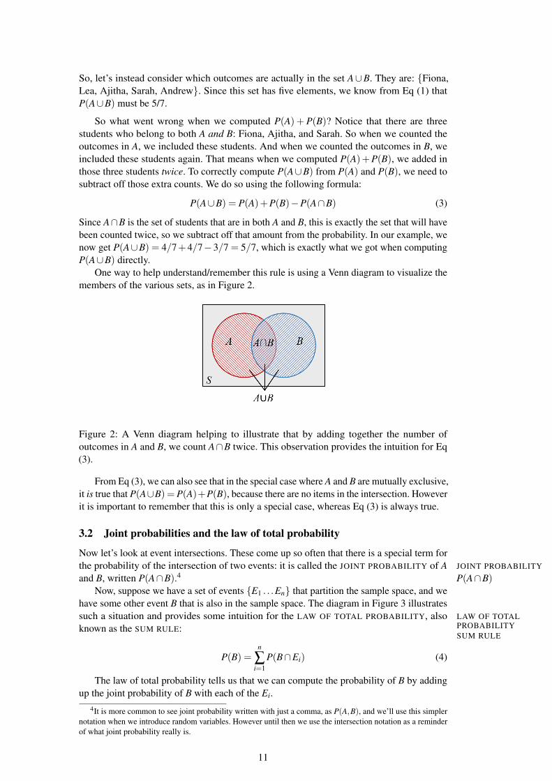
One way to help understand/remember this rule is using a Venn diagram to visualize themembers of the various sets, as in Figure 2.

Figure 2: A Venn diagram helping to illustrate that by adding together the number ofoutcomes in A and B, we count A∩B twice. This observation provides the intuition for Eq(3).

From Eq (3), we can also see that in the special case where A and B are mutually exclusive,it is true that P(A∪B) =P(A)+P(B), because there are no items in the intersection. Howeverit is important to remember that this is only a special case, whereas Eq (3) is always true.

3.2 Joint probabilities and the law of total probability

Now let’s look at event intersections. These come up so often that there is a special term forthe probability of the intersection of two events: it is called the JOINT PROBABILITY of A JOINT PROBABILITY

and B, written P(A∩B).4 P(A∩B)Now, suppose we have a set of events {E1 . . .En} that partition the sample space, and we

have some other event B that is also in the sample space. The diagram in Figure 3 illustratessuch a situation and provides some intuition for the LAW OF TOTAL PROBABILITY, also LAW OF TOTAL

PROBABILITYknown as the SUM RULE:SUM RULE

P(B) =n

∑i=1

P(B∩Ei) (4)

The law of total probability tells us that we can compute the probability of B by addingup the joint probability of B with each of the Ei.

4It is more common to see joint probability written with just a comma, as P(A,B), and we’ll use this simplernotation when we introduce random variables. However until then we use the intersection notation as a reminderof what joint probability really is.

11

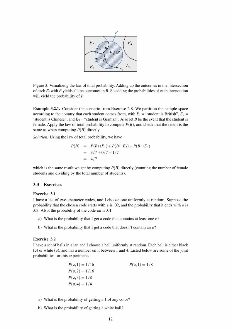
Figure 3: Visualizing the law of total probability. Adding up the outcomes in the intersectionof each Ei with B yields all the outcomes in B. So adding the probabilities of each intersectionwill yield the probability of B.

Example 3.2.1. Consider the scenario from Exercise 2.8. We partition the sample spaceaccording to the country that each student comes from, with E1 = “student is British”, E2 =“student is Chinese”, and E3 = “student is German”. Also let B be the event that the student isfemale. Apply the law of total probability to compute P(B), and check that the result is thesame as when computing P(B) directly.

Solution: Using the law of total probability, we have

P(B) = P(B∩E1)+P(B∩E2)+P(B∩E3)

= 3/7+0/7+1/7

= 4/7

which is the same result we get by computing P(B) directly (counting the number of femalestudents and dividing by the total number of students).

3.3 Exercises

Exercise 3.1I have a list of two-character codes, and I choose one uniformly at random. Suppose theprobability that the chosen code starts with s is .02, and the probability that it ends with s is.03. Also, the probability of the code ss is .01.

a) What is the probability that I get a code that contains at least one s?

b) What is the probability that I get a code that doesn’t contain an s?

Exercise 3.2I have a set of balls in a jar, and I choose a ball uniformly at random. Each ball is either black(b) or white (w), and has a number on it between 1 and 4. Listed below are some of the jointprobabilities for this experiment.

P(w,1) = 1/16 P(b,1) = 1/8

P(w,2) = 1/16

P(w,3) = 1/8

P(w,4) = 1/4

a) What is the probability of getting a 1 of any color?

b) What is the probability of getting a white ball?

12

c) What is the probability of getting a black ball?

d) What is the probability of getting either a black ball or a ball numbered 1?

Exercise 3.3Suppose I generate a 6-character password, where each character is chosen uniformly atrandom from of the 26 lowercase letters of English. What is the probability that my passwordcontains at least one repeated character, i.e., there is at least one character that occurs morethan once somewhere in the password? (Hint: extend the solution to Example 2.3.4 to solvethis problem.)

4 Conditional probabilities, independence, and Bayes’ Rule

4.1 Definition of conditional probability

CONDITIONAL PROBABILITY is one of the most important concepts of probability theory. CONDITIONALPROBABILITYA conditional probability expresses the probability that some event A will occur, given that

(conditioned on the fact that) event B occurred. The conditional probability of A given B,written P(A |B), where the | is pronounced “given”, is defined as5 P(A |B)

P(A |B) = P(A∩B)P(B)

. (5)

Example 4.1.1. Again let’s use the scenario from Exercise 2.8 of Section 2.5, with events A= “the student is male” and B = “the student is from the UK”. What is P(A |B)?Solution: In this case, A∩B is the set of male British students, so P(A∩B) = 1/7. P(B) = 4/7,so P(A |B) = 1/7

4/7 = 1/4.

Hopefully this answer makes sense to you: intuitively, the probability that the chosenstudent is male given that the student is British is simply the number of male students asa fraction of the number of British students, or 1/4. But again, it’s important to learn theformal rules of probability theory since not all problems you will be faced with are sostraightforward.

Example 4.1.2. Using the same A and B as in Ex 4.1.1, what is P(B |A)?

Solution: We have the same A∩B, so P(A∩B) = 1/7. P(A) = 3/7, so P(A |B) = 1/73/7 = 1/3.

This example illustrates the fact that conditional probabilities are not commutative:P(A |B) is not the same as P(B |A), and in general the two will not be equal.

4.2 The product rule and chain rule

If we rearrange the terms in the definition of conditional probability (Eq 5), we obtain thePRODUCT RULE, which allows us to compute joint probabilities from conditional probabili- PRODUCT RULE

ties:P(A∩B) = P(A |B) P(B). (6)

Since intersection is commutative, we could also write P(A∩B) = P(B∩A) = P(B |A) P(A).

Example 4.2.1. Suppose I have a jar of marbles, and I choose one uniformly at random.Each marble is either red (R), green (G), or blue (B). In two-thirds of the marbles, these colorsare solid (S), while in the remainder the colors are patchy. If I tell you that the probabilityof getting a red marble given that I have a solid-colored one is 1/2, can you compute the

5P(A |B) is undefined if P(B) = 0.

13

probability that my chosen marble is solid red?

Solution: Yes: P(R∩S) = P(R |S) P(S). We were told that P(R |S) = 1/2, and P(S) = 2/3,so P(R∩S) = (1/2)(2/3) = 1/3.

Example 4.2.2. Now suppose the probability of the marble being blue given that it’s patchyis 1/5. What is the probability of getting a patchy blue marble?

Solution: We were not given the probability of a patchy marble, but the previous examplestated that all marbles are either solid or patchy, and that P(S), the probability of a solid-colormarble, is 2/3. So we can compute the probability of a patchy marble as P(¬S) = 1−P(S) =1/3. Then P(B∩¬S) = P(B |¬S) P(¬S) = (1/5)(1/3) = 1/15.

One consequence of the product rule is an alternative formulation of the law of total prob-ability. We can use the product rule to replace the joint probabilities in (4) with conditionalprobabilities, thereby obtaining

P(B) =n

∑i=1

P(B |Ei) P(Ei). (7)

This version of the law of total probability is often useful in problems involving Bayes’ Rule(introduced below in Section 4.6).

The product rule can only handle the intersection of two events, but notice that we canapply it iteratively to expand the joint probability of several events into a product of severalconditional probabilities. For example:

P(A∩B∩C∩D) = P(A |B∩C∩D) P(B∩C∩D)

= P(A |B∩C∩D) P(B |C∩D) P(C∩D)

= P(A |B∩C∩D) P(B |C∩D) P(C |D) P(D)

where in each step, we expanded the final term using the product rule. This is possiblebecause a complex event such as B∩C∩D is still just an event: it can take the place of B inEq (6).

This iterative rewriting process is summarized in a general form called the CHAIN RULE: CHAIN RULE

P(E1∩E2∩ . . .∩En) =n

∏i=1

P(Ei |Ei+1∩ . . .∩En) (8)

4.3 Conditional probability distributions

Suppose we have a set of events {E1 . . .En} that partition the sample space, and we considerthe conditional probabilities of these events conditioned on some other event B, whereP(B)> 0. Then these conditional probabilities P(E1 |B) . . .P(En |B) form a distribution—theCONDITIONAL PROBABILITY DISTRIBUTION conditioned on B. We can show that this set CONDITIONAL

PROBABILITYDISTRIBUTION

forms a distribution by first showing that the sum of the probabilities is one:

n

∑i=1

P(Ei |B) =n

∑i=1

P(Ei∩B)P(B)

by defn of conditional probability

=1

P(B)

n

∑i=1

P(Ei∩B)

=1

P(B)P(B) by law of total probability

= 1 (9)

We also need to show that all the P(Ei |B) are between 0 and 1. We know that P(B) andeach P(Ei∩B) is between 0 and 1, because they are probabilities. Also, P(Ei∩B) cannot be

14

larger than P(B), because the intersection of B with another set can’t be larger than B. But ifP(Ei∩B)≤ P(B), and P(B)> 0 and P(Ei∩B)≥ 0, then P(Ei∩B)

P(B) must be between 0 and 1.Because a conditional probability distribution is a distribution, the rules for computing

probabilities that we discussed already apply just as well to conditional distributions, providedwe keep the conditioning event in all parts of the equation. In particular,

P(¬E |B) = 1−P(E |B) (10)

P(A∪B |C) = P(A |C)+P(B |C)−P(A∩B |C) (11)

Example 4.3.1. Using the same jar of marbles as in Examples 4.2.1 and 4.2.2, I give youone more piece of information: the probability of a green marble given a patchy marble is2/5. What’s the probability of a red marble given a patchy marble?

Solution: We now have a lot of different pieces of information to keep straight. Let’s firstwrite down all the information that was explicitly stated in each of the examples:

P(S) = 2/3 P(R |S) = 1/2 P(B |¬S) = 1/5

P(G |¬S) = 2/5

Notice that I have arranged the information so that each column forms part of a conditionaldistribution, conditioned on a different thing (either nothing, or S, or ¬S). We want to knowP(R |¬S), which would belong in the third column, and we also know that adding up all theitems in that distribution should equal one. But P(R |¬S) is the only item missing from thedistribution. Therefore, P(R |¬S) = 1− (P(B |¬S)+P(G |¬S)), or 2/5.

4.4 Conditional and joint probability tables

Another way of representing a conditional probability distribution is using a CONDITIONAL

PROBABILITY TABLE, or CPT. A CPT for the distribution conditioned on A has one column CONDITIONALPROBABILITY TABLEfor each event Ei in the partition. Each column is labelled with Ei and lists the value of

P(Ei |A). So, the CPT for ¬S before solving the previous example would be:

R G B2/5 1/5

This table makes it completely clear that R is the only missing value, and therefore canbe filled in with the value that makes the row sum to one.

Depending on what problem we are trying to solve, it may be more useful to constructa table listing joint probabilities rather than conditional probabilities (a JOINT PROBABIL-ITY TABLE, or JPT). This kind of table assumes we have two different partitions of the JOINT PROBABILITY

TABLEsample space, {D1 . . .Dn}, and {E1 . . .Em} (such as our partitions into solid/patchy andred/blue/green in the marble example).6 Each row in the table represents a Di, and eachcolumn represents an E j. The value in cell (i, j) is P(Di,E j).

Example 4.4.1. Construct a joint probability table for the scenario from Example 4.3.1,where the rows represent the S and ¬S events, and the columns represent the color events.Fill in the cells for which we have computed values already in previous examples, then fill inas many additional cells as possible given the other information we have so far.

Solution: The table initially looks like this, with the two values we computed in Examples4.2.1 and 4.2.2:

R G BS 1/3¬S 1/15

6It it is perfectly possible to have a joint distribution using more than two different partitions, but in that caseit is difficult to use the table respresentation.

15

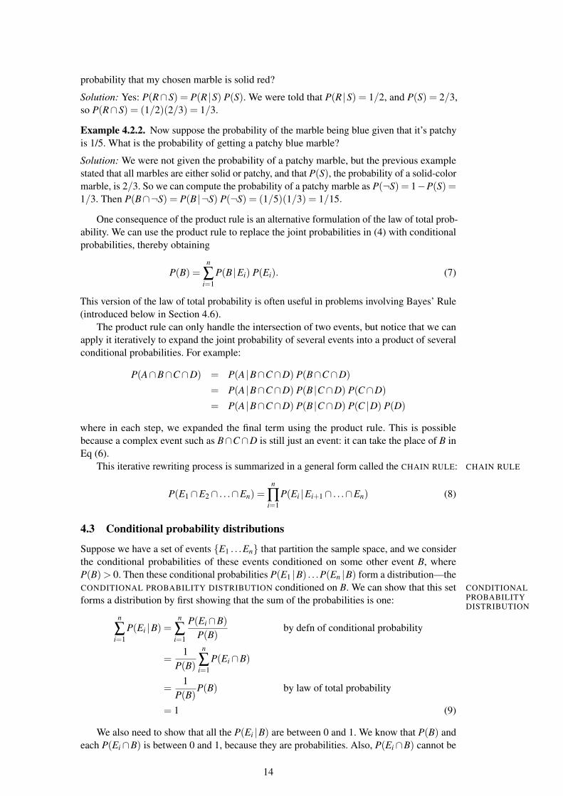
Using the information from Example 4.3.1, we can then compute two additional cells asP(R |¬S) P(¬S) and P(G |¬S) P(¬S). The table now looks like this:

R G BS 1/3¬S 2/15 2/15 1/15

Without further information, the two remaining cells remain unknown.

Notice that adding up the values in the ¬S row gives a value of 1/3, which is thesame value we computed earlier for P(¬S). This is not a coincidence! It is the law of totalprobability in action: look again at Eq 4 and you’ll see that adding up the values in anyrow or column of a JPT will give the probability of the event labelling that row or column.It is often useful to write down the summed probability of each row and column in themargins of the JPT as an aid to problem solving. The probabilities we end up with inthe margins are sometimes called MARGINAL PROBABILITIES, and using the law of total MARGINAL

PROBABILITIESprobability to compute one is called MARGINALIZATION. That is, if we are given P(S∩R),MARGINALIZATIONP(S∩G), and P(S∩B), then computing P(S) by summing the three joint probabilities would

be “marginalizing over” (or “marginalizing out”) the other events to obtain the marginalprobability of S.

Example 4.4.2. In our running example, suppose that P(B)= 1/5. Is this enough informationto fill in the rest of the JPT and its margins?

Solution: Yes. Let’s start by adding in the marginal probabilities that we know so far. Recallthat P(S) was given as 2/3, and P(¬S) was then computed as 1/3. So we have:

R G BS 1/3 2/3¬S 2/15 2/15 1/15 1/3

1/5

Now we can fill in P(R) = 1/3+2/15 = 7/15. Also, P(B∩S) = P(B)−P(B∩¬S) = 2/15:

R G BS 1/3 2/15 2/3¬S 2/15 2/15 1/15 1/3

7/15 1/5

We can now compute P(G∩ S) as P(S)−P(R∩S)−P(B∩S) and then P(G) as (G∩S)+P(G∩¬S). Or we could find P(G) first, as 1−P(R)−P(B), and compute P(G∩ S) fromthere. Either way, we end up with:

R G BS 1/3 1/5 2/15 2/3¬S 2/15 2/15 1/15 1/3

7/15 1/3 1/5 1

I added a 1 in the bottom right corner as a reminder that the values in the row margin, aswell as the values in the column margin, as well as the values in the non-marginal part of thetable, all add up to 1.

4.5 Independent events

In general, the conditional probability of an event is not the same as the unconditionalprobability of that event. We can see this from our marbles example, where we computedP(R) = 7/15 while P(R |S) = 1/2 and P(R |¬S) = 2/5.

16

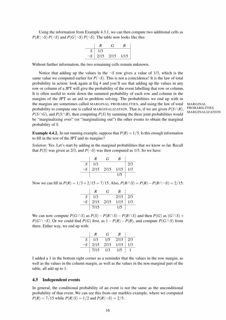
However, in some cases the conditional probability P(A |B) is equal to the unconditionalprobability P(A). That is, whether or not B occurs has no effect on the probability of Aoccurring. This is one way of defining the notion of INDEPENDENCE of two events. Two INDEPENDENCE

events A and B are INDEPENDENT EVENTS7 iff INDEPENDENTEVENTS

P(A |B) = P(A). (12)

By substituting in the definition of conditional probability from Eq (5) and rearranging theterms, we can equivalently state that events A and B are independent iff

P(A∩B) = P(A)P(B). (13)

Sometimes, it’s clear intuitively that two events are independent. For example, if I flipa coin twice, the event “I get a head on the first flip” is independent of the event “I get ahead on the second flip”. Or, it may be clear intuitively that two events are not independent.For example, the event that I arrive at work on time is clearly not independent of whetherI oversleep that morning. However, sometimes whether two events are independent is notintuitively obvious, and we need to use the definition of independence to determine theanswer.

Example 4.5.1. Using Eq (13) and the joint probability table computed in Example 4.4.2,determine which of the possible pairs of events are independent.

Solution: To solve this problem, for each pair of events we check whether the joint probabilityis equal to the product of the probabilities of the individual events. Put another way, is thevalue in cell (i, j) equal to the product of the marginal value in row i times the marginalvalue in column j? We find that P(S∩R) 6= P(S)P(R), so S and R are not independent.Similarly for (¬S∩R), (S∩G), and (¬S∩G). However, P(S∩B) = P(S)P(B), so S and Bare independent; and similarly for ¬S and B.

In fact, if we look back at the CPT we computed for ¬S at the beginning of Section 4.4,we see that P(B |¬S) = 1/5, which is equal to P(B) in the joint probability table margin. Sowe also could have determined these variables were independent using Eq (12).

4.6 Bayes’ Rule

We started off this tutorial by saying that probability theory is useful for prediction andinference. Perhaps the most important tool we’ll use for inference is BAYES’ RULE, also BAYES’ RULE

known as BAYES’ THEOREM. Bayes’ Rule is derived by replacing the P(A∩B) in the BAYES’ THEOREM

definition of conditional probability with P(B |A) P(A) (using the product rule). We obtain:

P(A |B) = P(B |A) P(A)P(B)

. (14)

Example 4.6.1. Suppose I have some playing cards in my hand from a standard deck, and itturns out that 1/4 of them are red cards (hearts or diamonds) and 3/8 are face cards (jack,queen, or king). Also, 1/2 of the red cards are face cards. If I choose one of the cards in myhand uniformly at random, and get a face card, what’s the probability that it is also a redcard?

Solution: Let R be the event that the card is red, and F be the event that it is a face card. We aretold that P(R) = 1/4, P(F) = 3/8, and P(F |R) = 1/2. (Notice which way the conditioninggoes! The problem said 1/2 of the red cards are faces, i.e., if we know the card is red, the

7Don’t confuse this definition with the related, but not identical definition of independent random variables,introduced later in Section 5.4.

17

probability that it’s a face is 1/2.) So,

P(R |F) =P(F |R)P(R)

P(F)

=(1/2)(1/4)

3/8= 1/3

In the previous example, the probability in the denominator P(F) was provided directly.However it’s very common (especially in real-life problems) that we aren’t given the valuein the denominator and must compute it from the conditional probabilities that we do know.Typically this can be done with the law of total probability (usually the version in Eq 7),as we’ll see in the following example. This example will also give us our first taste of anINFERENCE problem: a problem where we need to infer something that can’t be observed INFERENCE

directly (in this case, the presence or absence of a genetic marker) using information aboutsomething that can be observed directly (a test result) and the probabilistic relationshipbetween the two.

Example 4.6.2. In the general population, 1/1000 infants have a particular genetic markerthat is linked to cancer in later life. There is a test for this marker, but it isn’t perfect. If aninfant has the genetic marker, the test will always show a positive result. But it also has afalse positive rate of 1% (that is, 1% of infants who do not have the marker will still show apositive test result). If we test a particular infant and the test comes out positive, what’s theprobability that infant actually has the genetic marker?

Solution: Before answering this question, let’s determine the sample space of this sta-tistical experiment.8 It’s probably easiest to do that by working backwards. First, notethat the relevant events we’ll need to work with are G (infant has genetic marker) andT (test is positive).9 We will also want to talk about conditional and joint probabilitiesinvolving G and T , which implies that G and T are different subsets of the same sam-ple space. The easiest way, then, to define the sample space is as a set of four outcomes:{(pos,yes),(pos,no),(neg,yes),(neg,no)} where pos/neg indicates the test result andyes/no indicates the presence of the marker. G and T each pick out two of those outcomes.We are no longer working with equally likely outcomes here, but that’s ok because we neednot compute probabilities directly by counting outcomes, instead we have been given someprobabilities and need to compute other probabilities from those.

So, with the pedantic part out of the way, let’s work through the rest of the problem. Weare told that P(G) = .001, that P(T |¬G) = .01 (false positive rate), and that P(T |G) = 1(perfect detection). Now we want to compute P(G |T ). We begin by applying Bayes’ Rule:

P(G |T ) =P(T |G) P(G)

P(T )

We have been given the probabilities in the numerator, but not P(T ). However, we can applythe law of total probability in the denominator to split up P(T ) into other probabilities that

8This part is not strictly necessary to solve the problem and might seem pedantic, but I have found that whenstudents make errors in computing probabilities, it’s often because they haven’t thought about the sample space.So it’s good to get in the habit of considering the sample space for the problem you are working on.

9We could equally well define G and T as their complement events, “doesn’t have marker” and “test isnegative”. Try working through the solution on your own with that starting point and notice the result is the same.

18

we have already or can easily compute:

P(G |T ) = P(T |G) P(G)

P(T |G) P(G)+P(T |¬G) P(¬G)

=(1)(.001)

(1)(.001)+(.01)(.999)where P(¬G) = 1−P(G)

≈ .09

In other words, the probability that an infant with a positive test result actually has the geneticmarker is less than 10%.

Are you surprised that the probability is so low? It’s because even though the falsepositive rate is low, there are far more infants who don’t have the genetic marker than thosewho do, and altogether those infants generate quite a few false positives. However, it’s awell-known result from psychology that people are bad at estimating the answers to problemslike this, so if you were surprised, you are in good company!

In inference problems like this one, we often refer to P(G) as the PRIOR PROBABILITY PRIOR PROBABILITY

of G: the probability of that event before we make any observations. In contrast, P(G |T ) isthe POSTERIOR PROBABILITY of G: the probability of that event after observing some data POSTERIOR

PROBABILITY(in this case, the test result).

4.7 Exercises

Exercise 4.1In Example 4.6.1, we said that P(F |R) = 1/2 and P(R) = 1/4.

a) What is P(F ∩R)? What does this probability express (describe it in words)?

b) Are F and R independent? Why or why not?

Exercise 4.2Suppose we have events A, B, C, D, and are given the following probabilities:

P(A) = 0.5 P(A∩B) = 0.25

P(B) = 0.3 P(B |C) = 0.2

P(C) = 0.6 P(A |B∩C) = 0.1

P(D) = 0.4 P(B |A∩C) = 0.7

Compute the following probabilities.

a) P(A |B)

b) P(B∩C)

c) P(C |B)

d) P(A∩B∩C)

19

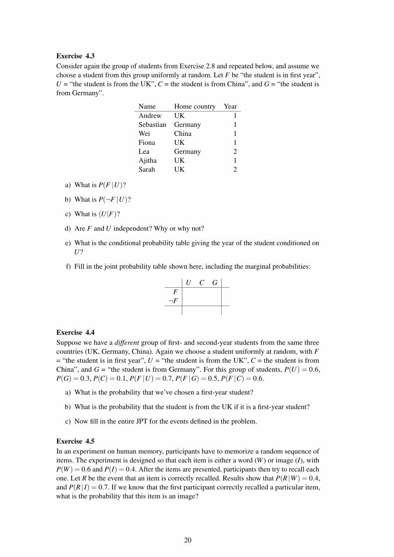
Exercise 4.3Consider again the group of students from Exercise 2.8 and repeated below, and assume wechoose a student from this group uniformly at random. Let F be “the student is in first year”,U = “the student is from the UK”, C = the student is from China”, and G = “the student isfrom Germany”.

Name Home country YearAndrew UK 1Sebastian Germany 1Wei China 1Fiona UK 1Lea Germany 2Ajitha UK 1Sarah UK 2

a) What is P(F |U)?

b) What is P(¬F |U)?

c) What is (U |F)?

d) Are F and U independent? Why or why not?

e) What is the conditional probability table giving the year of the student conditioned onU?

f) Fill in the joint probability table shown here, including the marginal probabilities:

U C GF¬F

Exercise 4.4Suppose we have a different group of first- and second-year students from the same threecountries (UK, Germany, China). Again we choose a student uniformly at random, with F= “the student is in first year”, U = “the student is from the UK”, C = the student is fromChina”, and G = “the student is from Germany”. For this group of students, P(U) = 0.6,P(G) = 0.3, P(C) = 0.1, P(F |U) = 0.7, P(F |G) = 0.5, P(F |C) = 0.6.

a) What is the probability that we’ve chosen a first-year student?

b) What is the probability that the student is from the UK if it is a first-year student?

c) Now fill in the entire JPT for the events defined in the problem.

Exercise 4.5In an experiment on human memory, participants have to memorize a random sequence ofitems. The experiment is designed so that each item is either a word (W ) or image (I), withP(W ) = 0.6 and P(I) = 0.4. After the items are presented, participants then try to recall eachone. Let R be the event that an item is correctly recalled. Results show that P(R |W ) = 0.4,and P(R | I) = 0.7. If we know that the first participant correctly recalled a particular item,what is the probability that this item is an image?

20

Exercise 4.6Suppose I want to choose a two-word name for a rock band via a random process. Thefirst word will be chosen with uniform probability from the set {yellow, purple, sordid,twisted}. The second word will be either quake, with probability 1/3, or revolution,with probability 2/3.

a) What’s the sample space for this experiment? How many outcomes are in it?

b) If I choose the first and second words independently, what is the probability that myrock band will be called yellow revolution?

c) Instead, I decide to condition the second word on the first. If the first word is a color,then I’ll pick quake as the second word with probability 1/6. Assuming I still want theoverall probability of a name with quake to be 1/3, what is the probability of quake ifthe first word is not a color? (Hint: use a joint probability table to help you answer thisquestion. You may not need to fill in the entire table.)

5 Random variables and discrete distributions

So far, we have been using distinct labels to refer to every event of interest. However, thisgets cumbersome, especially when we need to simultaneously refer to all the events in aparticular partition of the sample space. In practice, it’s much more common to work withrandom variables, as introduced in this section.

5.1 Definition of a random variable

A RANDOM VARIABLE (or RV) is a variable that represents all the possible events in some RANDOM VARIABLERVpartition of the sample space. Put another way, an RV has several possible values, with each

value being one event in a partition (and where the values cover all events in the partition). Wewill write random variables with uppercase letters, and their possible values with lowercaseletters or numbers.10

Example 5.1.1. Define a random variable X to represent the outcome flipping a fair coin,where this variable can take on two possible values (h or t) representing heads or tails. Whatis the distribution over X?

Solution: The distribution over an RV simply tells us the probability of each value, so thedistribution over X is P(X = h) = P(X = t) = 1/2.

We use the notation P(X) as a shorthand meaning “the entire distribution over X”, in P(X)contrast to P(X = x), which means “the probability that X takes the value x”. P(X = x)

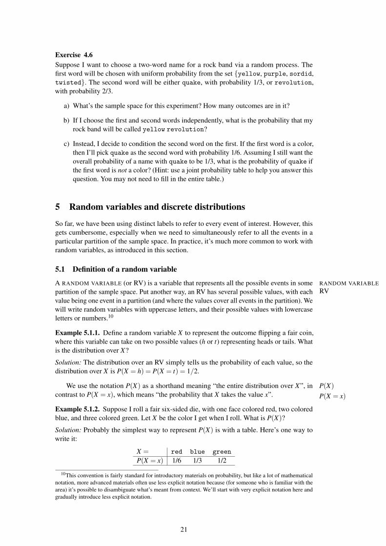
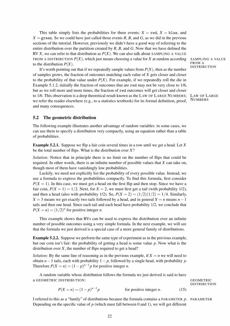
Example 5.1.2. Suppose I roll a fair six-sided die, with one face colored red, two coloredblue, and three colored green. Let X be the color I get when I roll. What is P(X)?

Solution: Probably the simplest way to represent P(X) is with a table. Here’s one way towrite it:

X = red blue green

P(X = x) 1/6 1/3 1/2

10This convention is fairly standard for introductory materials on probability, but like a lot of mathematicalnotation, more advanced materials often use less explicit notation because (for someone who is familiar with thearea) it’s possible to disambiguate what’s meant from context. We’ll start with very explicit notation here andgradually introduce less explicit notation.

21

This table simply lists the probabilities for three events: X = red, X = blue, andX = green. So we could have just called those events R, B, and G, as we did in the previoussections of the tutorial. However, previously we didn’t have a good way of referring to theentire distribution over the partition created by R, B, and G. Now that we have defined theRV X , we can refer to that distribution as P(X). We can also talk about SAMPLING A VALUE

FROM A DISTRIBUTION P(X), which just means choosing a value for X at random according SAMPLING A VALUEFROM ADISTRIBUTION

to the distribution P(X).It’s worth pointing out that if we repeatedly sample values from P(X), then as the number

of samples grows, the fraction of outcomes matching each value of X gets closer and closerto the probability of that value under P(X). For example, if we repeatedly roll the die inExample 5.1.2, initially the fraction of outcomes that are red may not be very close to 1/6,but as we roll more and more times, the fraction of red outcomes will get closer and closerto 1/6. This observation is a deep theoretical result known as the LAW OF LARGE NUMBERS; LAW OF LARGE

NUMBERSwe refer the reader elsewhere (e.g., to a statistics textbook) for its formal definition, proof,and many consequences.

5.2 The geometric distribution

The following example illustrates another advantage of random variables: in some cases, wecan use them to specify a distribution very compactly, using an equation rather than a tableof probabilities.

Example 5.2.1. Suppose we flip a fair coin several times in a row until we get a head. Let Xbe the total number of flips. What is the distribution over X?

Solution: Notice that in principle there is no limit on the number of flips that could berequired. In other words, there is an infinite number of possible values that X can take on,though most of them have vanishingly low probabilities.

Luckily, we need not explicitly list the probability of every possible value. Instead, weuse a formula to express the probabilities compactly. To find this formula, first considerP(X = 1). In this case, we must get a head on the first flip and then stop. Since we have afair coin, P(X = 1) = 1/2. Next, for X = 2, we must first get a tail (with probability 1/2),and then a head (also with probability 1/2). So, P(X = 2) = (1/2)(1/2) = 1/4. Similarly,X = 3 means we get exactly two tails followed by a head, and in general X = n means n−1tails and then one head. Since each tail and each head have probability 1/2, we conclude thatP(X = n) = (1/2)n for positive integer n.

This example shows that RVs can be used to express the distribution over an infinitenumber of possible outcomes using a very simple formula. In the next example, we will seethat the formula we just derived is a special case of a more general family of distributions.

Example 5.2.2. Suppose we perform the same type of experiment as in the previous example,but our coin isn’t fair: the probability of getting a head is some value p. Now what is thedistribution over X , the number of flips required to get a head?

Solution: By the same line of reasoning as in the previous example, if X = n we will need toobtain n−1 tails, each with probability 1− p, followed by a single head, with probability p.Therefore P(X = n) = (1− p)n−1 p for positive integer n.

A random variable whose distribution follows the formula we just derived is said to havea GEOMETRIC DISTRIBUTION: GEOMETRIC

DISTRIBUTION

P(X = n) = (1− p)n−1 p for positive integer n. (15)

I referred to this as a “family” of distributions because the formula contains a PARAMETER p. PARAMETER

Depending on the specific value of p (which must fall between 0 and 1), we will get different

22

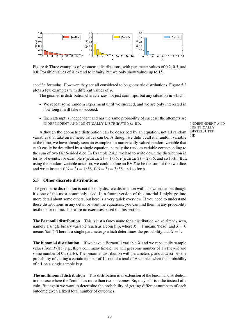
Figure 4: Three examples of geometric distributions, with parameter values of 0.2, 0.5, and0.8. Possible values of X extend to infinity, but we only show values up to 15.

specific formulas. However, they are all considered to be geometric distributions. Figure 5.2plots a few examples with different values of p.

The geometric distribution characterizes not just coin flips, but any situation in which:

• We repeat some random experiment until we succeed, and we are only interested inhow long it will take to succeed.

• Each attempt is independent and has the same probability of success: the attempts areINDEPENDENT AND IDENTICALLY DISTRIBUTED or IID. INDEPENDENT AND

IDENTICALLYDISTRIBUTEDIID

Although the geometric distribution can be described by an equation, not all randomvariables that take on numeric values can be. Although we didn’t call it a random variableat the time, we have already seen an example of a numerically valued random variable thatcan’t easily be described by a single equation, namely the random variable corresponding tothe sum of two fair 6-sided dice. In Example 2.4.2, we had to write down the distribution interms of events, for example P(sum is 2) = 1/36, P(sum is 3) = 2/36, and so forth. But,using the random variable notation, we could define an RV S to be the sum of the two dice,and write instead P(S = 2) = 1/36, P(S = 3) = 2/36, and so forth.

5.3 Other discrete distributions

The geometric distribution is not the only discrete distribution with its own equation, thoughit’s one of the most commonly used. In a future version of this tutorial I might go intomore detail about some others, but here is a very quick overview. If you need to understandthese distributions in any detail or want the equations, you can find them in any probabilitytextbook or online. There are no exercises based on this section.

The Bernoulli distribution This is just a fancy name for a distribution we’ve already seen,namely a single binary variable (such as a coin flip, where X = 1 means ‘head’ and X = 0means ‘tail’). There is a single parameter p which determines the probability that X = 1.

The binomial distribution If we have a Bernoulli variable X and we repeatedly samplevalues from P(X) (e.g., flip a coin many times), we will get some number of 1’s (heads) andsome number of 0’s (tails). The binomial distribution with parameters p and n describes theprobability of getting a certain number of 1’s out of a total of n samples when the probabilityof a 1 on a single sample is p.

The multinomial distribution This distribution is an extension of the binomial distributionto the case where the “coin” has more than two outcomes. So, maybe it is a die instead of acoin. But again we want to determine the probability of getting different numbers of eachoutcome given a fixed total number of outcomes.

23

The Poisson distribution This distribution has a single parameter, usually called λ

(lambda), the “rate”. One way to think about this distribution is as follows: we are countinghow often a particular thing happens. On average, that thing happens λ times within a certainfixed period of time, but the intervals between the occurrences are random. The Poissondistribution tells us the probability of that thing happening exactly x times with the fixedperiod. An example would be: we are counting the number of typos in each 1000 words oftext. On average, there are 5 typos per 1000 words. What is the probability that there areexactly 4 typos in the next 1000 words?

5.4 Restating the probability rules using random variables

As we’ve seen, there is a close relationship between random variables and partitions of thesample space into events, but the notation is slightly different. Since the random variablenotation is more commonly used, it’s worth going through each of the rules of probability andother tools we presented earlier to show how they apply when we’re using random variables.

Let’s assume we are working with a random variable X whose possible values are{x1,x2, . . . ,xn}. These values could be numeric (e.g., integers) or categorical (e.g., differentletters or different colors), and n could be a finite number or infinity. However, we assumethat the xi values are ENUMERABLE, which means that it is possible to create a one-to-one ENUMERABLE

mapping between these values and the integers (think of it as assigning a unique integer toeach xi value). This assumption means that X is a DISCRETE RANDOM VARIABLE, i.e., it DISCRETE RANDOM

VARIABLEhas a set of discrete possible values. Later we will consider continuous random variables,which can take on real-number values.

We can now (re)state the requirements for a DISCRETE PROBABILITY DISTRIBUTION or DISCRETEPROBABILITYDISTRIBUTION

PROBABILITY MASS FUNCTION as follows:

PROBABILITY MASSFUNCTION0≤ P(X = xi)≤ 1 (16)

n

∑i=1

P(X = xi) = 1 (17)

As a shorthand notation, instead of writing the values of an RV explicitly in a sum, suchas ∑

ni=1 P(X = xi), we will often just write ∑x P(X = x), which should be interpreted in the

same way: that is, as a sum in which x ranges over all possible values of X . In more advancedmaterials, you will often find that an even more concise notation is used: to indicate theprobability of an RV taking a particular value x, authors may just write P(x) rather thanP(X = x) as we have been doing. In this case, the above sum would be written as ∑x P(x).

Before going through the rest of the rules of probability, we introduce one more notationalvariant, this time for the joint probability of two random variables X and Y . We previouslyused the intersection symbol for joint probability, but it is more common (especially whenusing random variables) to use a comma instead, as in P(X = 1,Y = blue). And, just as P(X)refers to the distribution over X , we refer to the entire JOINT PROBABILITY DISTRIBUTION JOINT PROBABILITY

DISTRIBUTIONover X and Y as P(X ,Y ): you can think of it as referring to the entire JPT.P(X ,Y )

Example 5.4.1. Rewrite the JPT from Example 4.4.2 using random variable notation, withX representing the color of the marble, and Y representing the pattern (solid or patchy).

Solution:

X = r X = g X = b

Y = solid 1/3 1/5 2/15 2/3Y = patchy 2/15 2/15 1/15 1/3

7/15 1/3 1/5

With all the notation out of the way, we now restate several of the other rules of probability,using both the verbose and concise notations.

24

verbose conciseP(X = x) = 1−P(X 6= x) P(x) = 1−P(¬x) complement

(18)

P(X = x) = ∑y

P(X = x,Y = y) P(x) = ∑y

P(x,y) law of total prob

(19)

P(X = x |Y = y) =P(X = x,Y = y)

P(Y = y)P(x |y) = P(x,y)

P(y)defn of cond prob

(20)

P(X = x,Y = y) = P(X = x |Y = y)P(y) P(x,y) = P(x |y)P(y) product rule(21)

P(X = x |Y = y) =P(Y = y |X = x)P(X = x)

P(Y = y)P(x |y) = P(y |x)P(x)

P(y)Bayes’ Rule

(22)

So far, all of these rules are straightforwardly equivalent to the ones we saw earlier.However, there are a couple of places where we need to be more careful. The first of theseis when referring to a CONDITIONAL PROBABILITY DISTRIBUTION. We can refer to a CONDITIONAL

PROBABILITYDISTRIBUTION

(marginal) distribution as P(X) and a joint distribution as P(X ,Y ). But it is incorrect to writeP(X |Y ), because a conditional distribution has to be conditioned on a particular event. Validways to refer to a conditional distribution include P(X |Y = y) or P(X |y). P(X |Y = y)

The second case we need to be careful about is the definition of INDEPENDENT RANDOM

VARIABLES. We say that two RVs X and Y are independent iff, for all values of x and y, INDEPENDENTRANDOM VARIABLES

P(X = x,Y = y) = P(X = x)P(Y = y). (23)

This is a more general statement than independence of two events. We can say that the eventsX = x and Y = y are independent iff Eq (23) is true for those particular events, regardless ofwhether other outcomes of X and Y obey Eq (23). But for the random variables X and Y tobe independent, all possible outcomes of X and Y must obey Eq (23).

Example 5.4.2. Are the RVs X and Y from Example 5.4.1 independent?

Solution: No. Recall that in Example 4.5.1 we found that whether the marble is blue isindependent of whether it’s solid or patchy. So those particular events are independent.However, we also found that the other two colors were not independent of the solid/patchyevents. So overall, X and Y are not independent.

If we had not already determined the independence of the various events in the JPT inExample 4.5.1, we would only need to find a single case where Eq (23) fails to know that theRVs are not independent. For example, P(X = r,Y = patchy) 6= P(X = r)P(Y = patchy).

5.5 Working with more than two variables

In the previous sections, we mostly assumed probability distributions are only over oneor two variables. However, we may want to define joint distributions over more than twovariables, such as P(X ,Y,Z). And if we do that, then we can also condition on one or moreof those variables, for example looking at P(X ,Y |Z = z) or P(X |Y = y,Z = z).

Example 5.5.1. Returning to our marble example, assume we start with the same jar ofmarbles as in 5.4.1, but we add some new marbles to the jar. These new marbles have thesame joint distribution over X (color) and Y (pattern) as the existing ones, but there are

25

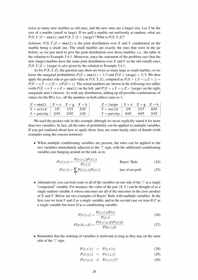
twice as many new marbles as old ones, and the new ones are a larger size. Let Z be thesize of a marble (small or large). If we pull a marble out uniformly at random, what areP(X ,Y |Z = small) and P(X ,Y |Z = large)? What is P(X ,Y,Z)?

Solution: P(X ,Y |Z = small) is the joint distribution over X and Y conditioned on themarble being a small one. The small marbles are exactly the ones that were in the jarbefore, so we just need to give the joint distribution over those marbles, i.e., the table inthe solution to Example 5.4.1. Moreover, since the statement of the problem says that thenew (large) marbles have the same joint distribution over X and Y as the old (small) ones,P(X ,Y |Z = large) is also given by the solution to Example 5.4.1.

As for P(X ,Y,Z), the question says there are twice as many large as small marbles, so weknow the marginal probabilities P(Z = small) = 1/3 and P(Z = large) = 2/3. We thenapply the product rule to get each value in P(X ,Y,Z), computed as P(X = x,Y = y,Z = z) =P(X = x,Y = y |Z = z)P(Z = z). The actual numbers are shown in the following two tables(with P(X = x,Y = y,Z = small) on the left, and P(X = x,Y = y,Z = large) on the right;marginals aren’t shown). As with any distribution, adding up all possible combinations ofvalues for the RVs (i.e., all the numbers in both tables) sums to 1.

Z = small X = r X = g X = b

Y = solid 1/9 1/15 2/45Y = patchy 2/45 2/45 1/45

Z = large X = r X = g X = b

Y = solid 2/9 2/15 4/45Y = patchy 4/45 4/45 2/45

We used the product rule in this example although we never explicitly stated it for morethan two variables. In fact, all the rules of probability can be applied to multiple variables.If you get confused about how to apply them, here are some handy rules of thumb (withexamples using the concise notation):

• When multiple conditioning variables are present, the rules can be applied to thetwo variables immediately adjacent to the ‘|’ sign, with the additional conditioningvariables just hanging around on the end, as in:

P(x |y,z) = P(y |x,z)P(x |z)P(y |z)

Bayes’ Rule (24)

P(x |z) = ∑y

P(x |y,z)P(y |z) law of tot prob (25)

• Alternatively, you can treat some or all of the variables on one side of the ‘|’ as a single“compound” variable. For instance, the value of the pair (X ,Y ) can be thought of as asingle random variable A whose outcomes are all of the outcomes in the cross productof X and Y . Below are two examples of Bayes’ Rule with multiple variables. In thefirst case we treat Y and Z as a single variable, and in the second case we treat B,C asa single variable but leave D as a conditioning variable.

P(x |y,z) = P(y,z |x)P(x)P(y,z)

(26)

P(a |b,c,d) = P(b,c |a,d)P(a |d)P(b,c |d)

(27)

• Remember that the ordering of variables is irrelevant as long as they stay on the sameside of the ‘|’ sign:

P(x,y |z) = P(y,x |z) (28)

P(x |y,z) = P(x |z,y) (29)

P(x |y,z) 6= P(x,y |z)!! (30)

26

Finally, we introduce the notion of CONDITIONAL INDEPENDENCE, which relies on CONDITIONALINDEPENDENCEmultiple variables. Informally, two RVs X and Y are conditionally independent given Z

iff once we know the value of Z, X and Y are independent. More formally, X and Y areconditionally independent given Z iff for all values of x, y, and z,

P(X = x,Y = y |Z = z) = P(X = x |Z = z)P(Y = y |Z = z) (31)

Example 5.5.2. Let X and Y be variables representing whether I stay up late and whetherI show up on time for my 9 a.m. class. Let Z represent whether I left my house on time.Intuitively, are X and Y independent? Are they conditionally independent given Z?

Solution: They are not independent: presumably I’m less likely to arrive on time if I stayedup late. But, if we know whether I left the house on time, they are independent: knowing if Istayed up late or not is now irrelevant. So, X and Y are conditionally independent given Z.

Conditional independence (or the assumption of conditional independence) comes upa lot in machine learning and NLP. One place where it can be useful is if we are trying toclassify items into different categories based on the features of those items, another exampleof probabilistic inference.

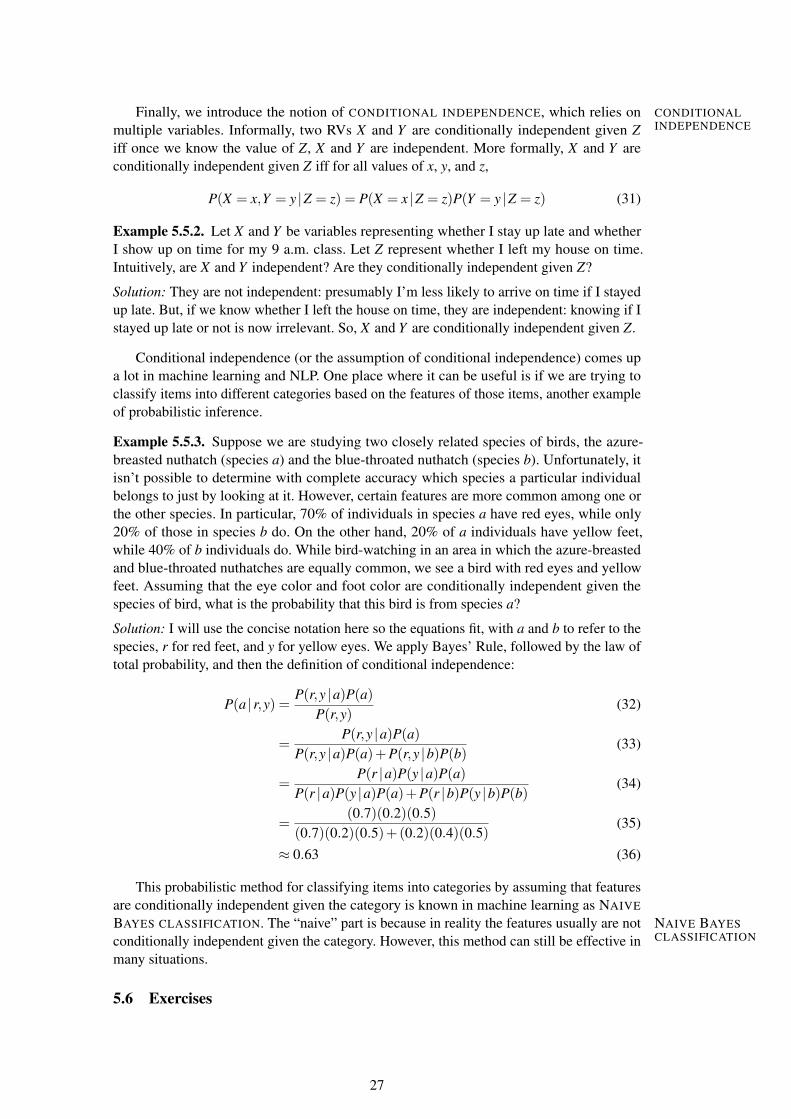
Example 5.5.3. Suppose we are studying two closely related species of birds, the azure-breasted nuthatch (species a) and the blue-throated nuthatch (species b). Unfortunately, itisn’t possible to determine with complete accuracy which species a particular individualbelongs to just by looking at it. However, certain features are more common among one orthe other species. In particular, 70% of individuals in species a have red eyes, while only20% of those in species b do. On the other hand, 20% of a individuals have yellow feet,while 40% of b individuals do. While bird-watching in an area in which the azure-breastedand blue-throated nuthatches are equally common, we see a bird with red eyes and yellowfeet. Assuming that the eye color and foot color are conditionally independent given thespecies of bird, what is the probability that this bird is from species a?

Solution: I will use the concise notation here so the equations fit, with a and b to refer to thespecies, r for red feet, and y for yellow eyes. We apply Bayes’ Rule, followed by the law oftotal probability, and then the definition of conditional independence:

P(a |r,y) = P(r,y |a)P(a)P(r,y)

(32)

=P(r,y |a)P(a)

P(r,y |a)P(a)+P(r,y |b)P(b)(33)

=P(r |a)P(y |a)P(a)

P(r |a)P(y |a)P(a)+P(r |b)P(y |b)P(b)(34)

=(0.7)(0.2)(0.5)

(0.7)(0.2)(0.5)+(0.2)(0.4)(0.5)(35)

≈ 0.63 (36)

This probabilistic method for classifying items into categories by assuming that featuresare conditionally independent given the category is known in machine learning as NAIVE

BAYES CLASSIFICATION. The “naive” part is because in reality the features usually are not NAIVE BAYESCLASSIFICATIONconditionally independent given the category. However, this method can still be effective in

many situations.

5.6 Exercises

27

Exercise 5.1Suppose I decide to generate a “word” as follows: I start by generating the character a. Then,with probability q, I generate a single b and stop, otherwise I generate another a and keepgoing. I continue this process, always either generating a single b with probability q andstopping, or generating an a and continuing.

a) What are the possible words I might generate using this process?

b) If L is a random variable representing the length of a word, give an equation forP(L = n). What kind of distribution does L have?

c) If q = 0.3, what is the probability that my generated word has 4 characters? What isthe probability of generating the word aaab?

Exercise 5.2Now suppose I have five different characters that can be in my word (a, b, c, d, e). Asbefore, I start by generating the character a. Then, with probability q, I generate a b and stop,otherwise I choose one of the other four characters uniformly at random and keep going.I continue this process, always either generating a b with probability q and stopping, orchoosing one of the other four characters uniformly at random and continuing.

a) What are the possible words I might generate using this process?

b) If L is a random variable representing the length of a word, give an equation forP(L = n). How does it differ from the equation found in Exercise 5.1?

c) If q = 0.3, what is the probability that my generated word has 4 characters? What isthe probability of generating the word aaab? Are your answers different to those inExercise 5.1? Why?

d) Again assuming q = 0.3, what is the probability of generating the word aaab giventhat I generate a 4-character word?

[More exercises to be added]

6 Expectation and variance

6.1 Definitions

When a random variable takes on numeric values, it can be useful to consider what theaverage or mean value of that variable is. That is: suppose we sample many values for an RVX (so that, by the Law of Large Numbers, the fraction of samples with value x matches theprobability of x). Adding up all the values we got and dividing by the number of samplesyields the average value we got for X .

Example 6.1.1. Suppose I offer to play a game with you. You roll two dice, and I’ll pay you£4 if you get a 6 or 11, but you pay me £1 otherwise. If we played this game many times in arow, who would end up winning more money? On average, how much would they win pergame?

Solution: Let X be the number of pounds you win on a single dice roll, so X can beeither 4 or -1. P(X = 4) is equal to the probability of rolling either 6 or 11. In Exercise2.3 you computed these as 5/36 and 2/36, respectively (you did do the excercise, didn’tyou?), and they are disjoint events, so P(X = 4) = 5/36+2/36 = 7/36. That leaves P(X =−1) = 1− 7/36 = 29/36. So over many games, you’d expect to win £4 7/36 of the time,

28

and lose £1 29/36 of the time. Altogether, your winnings over N games would be about(4)(7N/36)− (1)(29N/36) =−N/36 pounds. So I win more money, by an average of about3 pence for each game.

In the previous example, we literally took the average over a large number of samples ofX . However, even if we don’t take lots of samples, we can still say that, on average, we’dexpect the value of a single sample to be the same as the actual average over lots of samples.This idea leads to the definition of the EXPECTED VALUE or EXPECTATION of a random EXPECTED VALUE

EXPECTATIONvariable X , written E[X ] and formally defined as

E[X ] = ∑x

x ·P(X = x) (37)

Since E[X ] is really just the MEAN value for X , if it’s clear which X is being referred to, E[X ] MEAN

may also be wrtten simply as µ (pronounced “myoo”)—an abbreviation for “mean”. µRegardless of notation, Eq (37) defines the expected value of X as the sum of the

probability of each possible X value times the value itself. If we run an experiment N times,we can expect the sum of the X values to be about N ·E[X ].

Example 6.1.2. A contestant on a game show wins $1000. Then the host presents two boxes.In one box is a label marked “double” and in the other “nothing”. The contestant may, if shewishes, choose one of the boxes without seeing their contents. If she chooses the “double”box, she’ll get another $1000, but if she chooses “nothing”, she’ll lose the $1000 she alreadywon. If X is the additional amount she gets by taking the choice, what is E[X ]? Should shechoose a box, or just keep the money she has?

Solution: We have P(X = 1000) = 1/2 and P(X =−1000) = 1/2. So E[X ] = 1000(1/2)−1000(1/2) = 0. Of course, if she doesn’t choose a box, her expected additional winnings arealso 0. So, if the only consideration is her expected total winnings, it makes no difference ifshe decides to choose a box or not. Of course there are other psychological factors that mightbe important, such as whether the contestant likes to take risks. There are also mathematicaldifferences between the two choices, one of which we’ll return to shortly.

In addition to computing the expectation of an RV X , sometimes it’s useful to computethe expectation of a function of X , f (X), to give us the average value of the function:

E[ f (X)] = ∑x

f (x) ·P(X = x). (38)

Example 6.1.3. I offer to let you roll a single die, and will give you a number of poundsequal to the square of the number that comes up. How much would you expect to win byplaying this game?

Solution: Solution: If X is the number that comes up, the expected value of your winnings, inpounds, is

E[X2] = (1/6)(12)+(1/6)(22)+(1/6)(32) (39)

+(1/6)(42)+(1/6)(52)+(1/6)(62)

= 91/6 (40)

or about £15.17.

Let’s now return to the example of the contestant on the game show. We said there was nodifference in expected winnings if she decides to choose a box, or sticks with her $1000. Butclearly there’s something different in these two cases. One way to describe that something isusing the concept of VARIANCE. The variance of an RV tells us, for any given sample, how VARIANCE

far away from the expected value is the result likely to be? The variance of X is defined as

Var[X ] = E[(X−E[X ])2]. (41)

29

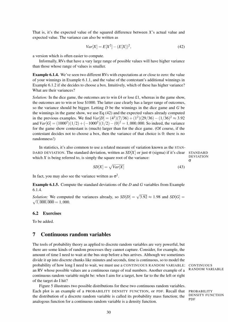
That is, it’s the expected value of the squared difference between X’s actual value andexpected value. The variance can also be written as

Var[X ] = E[X2]− (E[X ])2, (42)

a version which is often easier to compute.Informally, RVs that have a vary large range of possible values will have higher variance

than those whose range of values is smaller.

Example 6.1.4. We’ve seen two different RVs with expectations at or close to zero: the valueof your winnings in Example 6.1.1, and the value of the contestant’s additional winnings inExample 6.1.2 if she decides to choose a box. Intuitively, which of these has higher variance?What are their variances?

Solution: In the dice game, the outcomes are to win £4 or lose £1, whereas in the game show,the outcomes are to win or lose $1000. The latter case clearly has a larger range of outcomes,so the variance should be bigger. Letting D be the winnings in the dice game and G bethe winnings in the game show, we use Eq (42) and the expected values already computedin the previous examples. We find Var[D] = (42)(7/36)+ (12)(29/36)− (1/36)2 ≈ 3.92and Var[G] = (10002)(1/2)+(−10002)(1/2)− (0)2 = 1,000,000. So indeed, the variancefor the game show contestant is (much) larger than for the dice game. (Of course, if thecontestant decides not to choose a box, then the variance of that choice is 0: there is norandomness!)

In statistics, it’s also common to use a related measure of variation known as the STAN-DARD DEVIATION. The standard deviation, written as SD[X ] or just σ (sigma) if it’s clear STANDARD

DEVIATIONσ

which X is being referred to, is simply the square root of the variance:

SD[X ] =√

Var[X ] (43)

In fact, you may also see the variance written as σ2.

Example 6.1.5. Compute the standard deviations of the D and G variables from Example6.1.4.

Solution: We computed the variances already, so SD[D] =√

3.92 ≈ 1.98 and SD[G] =√1,000,000 = 1,000.

6.2 Exercises

To be added.

7 Continuous random variables

The tools of probability theory as applied to discrete random variables are very powerful, butthere are some kinds of random processes they cannot capture. Consider, for example, theamount of time I need to wait at the bus stop before a bus arrives. Although we sometimesdivide it up into discrete chunks like minutes and seconds, time is continuous, so to model theprobability of how long I need to wait, we must use a CONTINUOUS RANDOM VARIABLE: CONTINUOUS

RANDOM VARIABLEan RV whose possible values are a continuous range of real numbers. Another example of acontinuous random variable might be: when I aim for a target, how far to the the left or rightof the target do I hit?

Figure 5 illustrates two possible distributions for these two continuous random variables.Each plot is an example of a PROBABILITY DENSITY FUNCTION, or PDF. Recall that PROBABILITY

DENSITY FUNCTIONPDF

the distribution of a discrete random variable is called its probability mass function; theanalogous function for a continuous random variable is a density function.

30

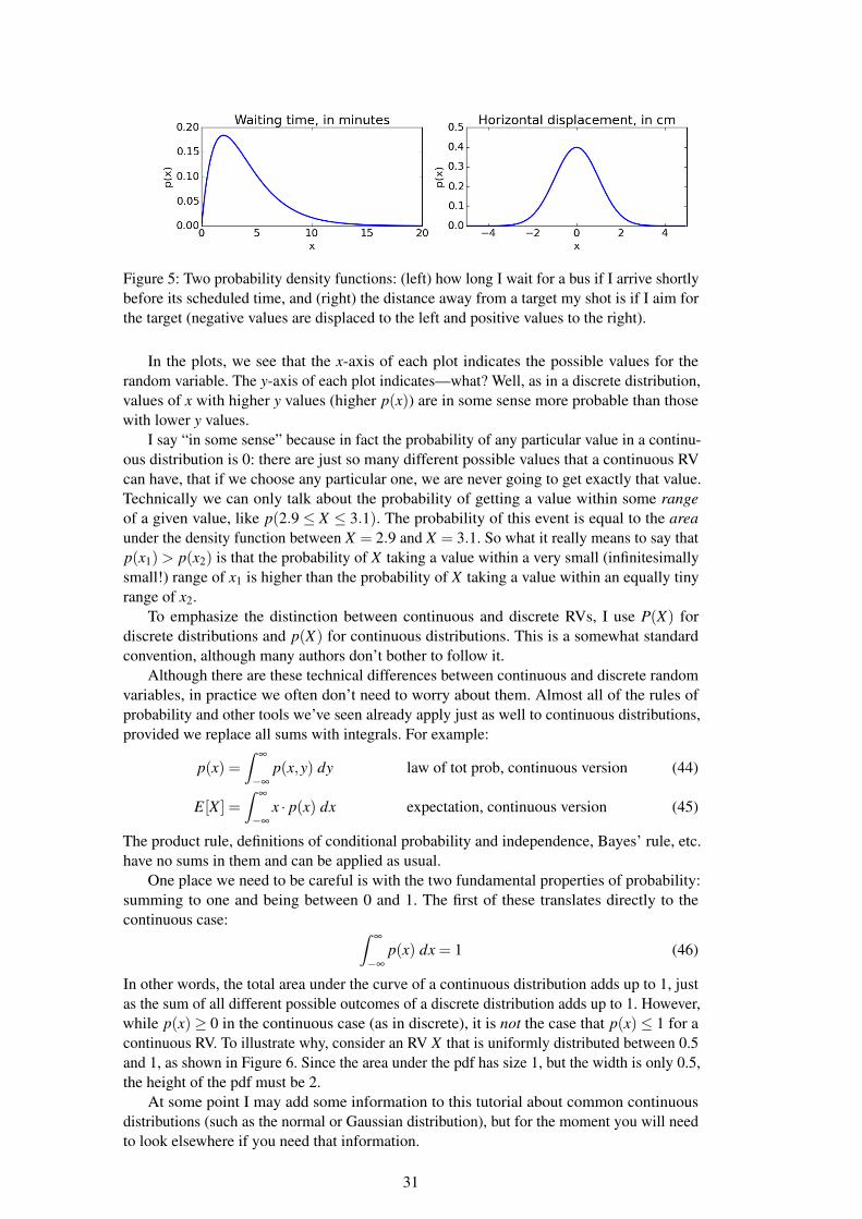
Figure 5: Two probability density functions: (left) how long I wait for a bus if I arrive shortlybefore its scheduled time, and (right) the distance away from a target my shot is if I aim forthe target (negative values are displaced to the left and positive values to the right).

In the plots, we see that the x-axis of each plot indicates the possible values for therandom variable. The y-axis of each plot indicates—what? Well, as in a discrete distribution,values of x with higher y values (higher p(x)) are in some sense more probable than thosewith lower y values.

I say “in some sense” because in fact the probability of any particular value in a continu-ous distribution is 0: there are just so many different possible values that a continuous RVcan have, that if we choose any particular one, we are never going to get exactly that value.Technically we can only talk about the probability of getting a value within some rangeof a given value, like p(2.9 ≤ X ≤ 3.1). The probability of this event is equal to the areaunder the density function between X = 2.9 and X = 3.1. So what it really means to say thatp(x1)> p(x2) is that the probability of X taking a value within a very small (infinitesimallysmall!) range of x1 is higher than the probability of X taking a value within an equally tinyrange of x2.

To emphasize the distinction between continuous and discrete RVs, I use P(X) fordiscrete distributions and p(X) for continuous distributions. This is a somewhat standardconvention, although many authors don’t bother to follow it.

Although there are these technical differences between continuous and discrete randomvariables, in practice we often don’t need to worry about them. Almost all of the rules ofprobability and other tools we’ve seen already apply just as well to continuous distributions,provided we replace all sums with integrals. For example:

p(x) =∫

∞

−∞

p(x,y) dy law of tot prob, continuous version (44)

E[X ] =∫

∞

−∞

x · p(x) dx expectation, continuous version (45)

The product rule, definitions of conditional probability and independence, Bayes’ rule, etc.have no sums in them and can be applied as usual.

One place we need to be careful is with the two fundamental properties of probability:summing to one and being between 0 and 1. The first of these translates directly to thecontinuous case: ∫

∞

−∞

p(x) dx = 1 (46)

In other words, the total area under the curve of a continuous distribution adds up to 1, justas the sum of all different possible outcomes of a discrete distribution adds up to 1. However,while p(x)≥ 0 in the continuous case (as in discrete), it is not the case that p(x)≤ 1 for acontinuous RV. To illustrate why, consider an RV X that is uniformly distributed between 0.5and 1, as shown in Figure 6. Since the area under the pdf has size 1, but the width is only 0.5,the height of the pdf must be 2.

At some point I may add some information to this tutorial about common continuousdistributions (such as the normal or Gaussian distribution), but for the moment you will needto look elsewhere if you need that information.

31

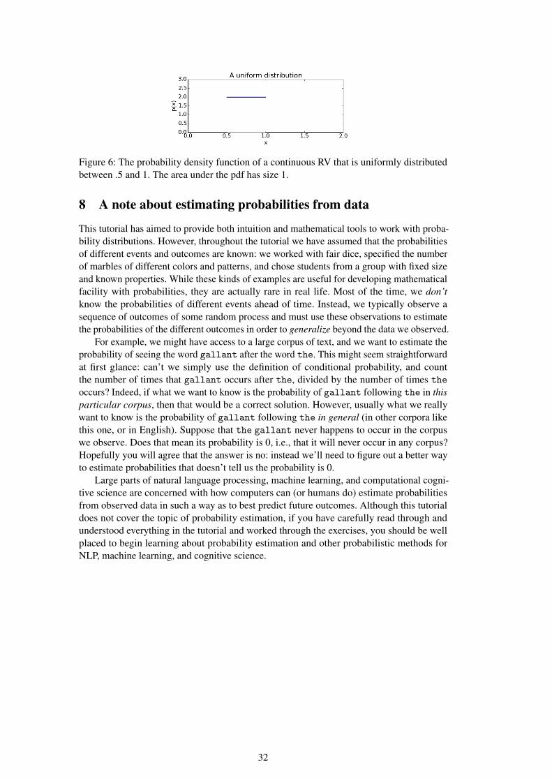
Figure 6: The probability density function of a continuous RV that is uniformly distributedbetween .5 and 1. The area under the pdf has size 1.

8 A note about estimating probabilities from data

This tutorial has aimed to provide both intuition and mathematical tools to work with proba-bility distributions. However, throughout the tutorial we have assumed that the probabilitiesof different events and outcomes are known: we worked with fair dice, specified the numberof marbles of different colors and patterns, and chose students from a group with fixed sizeand known properties. While these kinds of examples are useful for developing mathematicalfacility with probabilities, they are actually rare in real life. Most of the time, we don’tknow the probabilities of different events ahead of time. Instead, we typically observe asequence of outcomes of some random process and must use these observations to estimatethe probabilities of the different outcomes in order to generalize beyond the data we observed.

For example, we might have access to a large corpus of text, and we want to estimate theprobability of seeing the word gallant after the word the. This might seem straightforwardat first glance: can’t we simply use the definition of conditional probability, and countthe number of times that gallant occurs after the, divided by the number of times theoccurs? Indeed, if what we want to know is the probability of gallant following the in thisparticular corpus, then that would be a correct solution. However, usually what we reallywant to know is the probability of gallant following the in general (in other corpora likethis one, or in English). Suppose that the gallant never happens to occur in the corpuswe observe. Does that mean its probability is 0, i.e., that it will never occur in any corpus?Hopefully you will agree that the answer is no: instead we’ll need to figure out a better wayto estimate probabilities that doesn’t tell us the probability is 0.

Large parts of natural language processing, machine learning, and computational cogni-tive science are concerned with how computers can (or humans do) estimate probabilitiesfrom observed data in such a way as to best predict future outcomes. Although this tutorialdoes not cover the topic of probability estimation, if you have carefully read through andunderstood everything in the tutorial and worked through the exercises, you should be wellplaced to begin learning about probability estimation and other probabilistic methods forNLP, machine learning, and cognitive science.

32

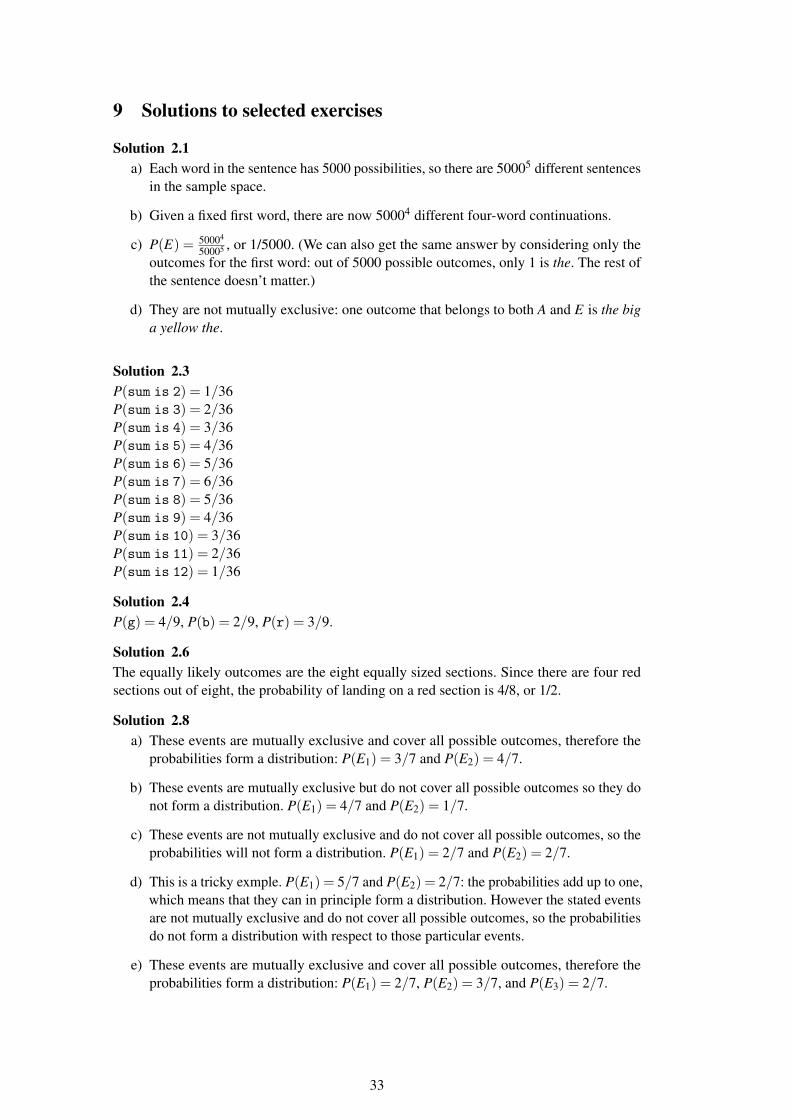
9 Solutions to selected exercises

Solution 2.1a) Each word in the sentence has 5000 possibilities, so there are 50005 different sentences

in the sample space.

b) Given a fixed first word, there are now 50004 different four-word continuations.

c) P(E) = 50004

50005 , or 1/5000. (We can also get the same answer by considering only theoutcomes for the first word: out of 5000 possible outcomes, only 1 is the. The rest ofthe sentence doesn’t matter.)

d) They are not mutually exclusive: one outcome that belongs to both A and E is the biga yellow the.

Solution 2.3P(sum is 2) = 1/36P(sum is 3) = 2/36P(sum is 4) = 3/36P(sum is 5) = 4/36P(sum is 6) = 5/36P(sum is 7) = 6/36P(sum is 8) = 5/36P(sum is 9) = 4/36P(sum is 10) = 3/36P(sum is 11) = 2/36P(sum is 12) = 1/36

Solution 2.4P(g) = 4/9, P(b) = 2/9, P(r) = 3/9.

Solution 2.6The equally likely outcomes are the eight equally sized sections. Since there are four redsections out of eight, the probability of landing on a red section is 4/8, or 1/2.

Solution 2.8a) These events are mutually exclusive and cover all possible outcomes, therefore the

probabilities form a distribution: P(E1) = 3/7 and P(E2) = 4/7.

b) These events are mutually exclusive but do not cover all possible outcomes so they donot form a distribution. P(E1) = 4/7 and P(E2) = 1/7.

c) These events are not mutually exclusive and do not cover all possible outcomes, so theprobabilities will not form a distribution. P(E1) = 2/7 and P(E2) = 2/7.

d) This is a tricky exmple. P(E1) = 5/7 and P(E2) = 2/7: the probabilities add up to one,which means that they can in principle form a distribution. However the stated eventsare not mutually exclusive and do not cover all possible outcomes, so the probabilitiesdo not form a distribution with respect to those particular events.

e) These events are mutually exclusive and cover all possible outcomes, therefore theprobabilities form a distribution: P(E1) = 2/7, P(E2) = 3/7, and P(E3) = 2/7.

33

Solution 3.1a) Let A = “starts with S” and B = “ends with S”. Then “at least one S” is A∪B. And

P(A∪B) = P(A)+P(B)−P(A,B) = .02+ .03− .01 = .04.

b) This event is the complement of the previous one, so its probability is 1− .04, or .96.

Solution 4.1a) P(F ∩R) = P(F |R) P(R) = 1/8. This is the probability that the chosen card is a red

face card.

b) They are not independent because P(R)P(F) 6= P(R∩F).

Solution 4.3a) P(F |U) = P(F∩U)

P(U) = 3/74/7 = 3/4

b) P(¬F |U) = 1−P(F |U) = 1/4

c) 3/5

d) No, because P(F |U) 6= P(F).

e) F ¬F3/4 1/4

f) U C GF 3/7 1/7 1/7 5/7¬F 1/7 0 1/7 2/7

4/7 1/7 2/7

Solution 4.5

P(I |R) =P(R | I)P(I)

P(R)

=P(R | I)P(I)

P(R∩ I)+P(R∩W )

=P(R | I)P(I)

P(R | I)P(I)+P(R |W )P(W )

=(0.7)(0.4)

(0.7)(0.4)+(0.4)(0.6)≈ .54

Solution 5.1a) The words are sequences of characters consisting of one or more a’s followed by

exactly one b.

b) The equation is P(L = n) = (1− q)n−2(q). The distribution is nearly a geometricdistribution, except the exponent is n−2 instead of n−1 because we always start withan a. Put another way, the distribution over lengths after the first character (i.e., overL−1) is geometric with parameter q.

c) Both are equal to (0.7)2(0.3)≈ 0.15

34