basic concepts of enriched category theory …€¦ · · 2015-05-22have allowed the production...
TRANSCRIPT

Reprints in Theory and Applications of Categories, No. 10, 2005.
BASIC CONCEPTS OFENRICHED CATEGORY THEORY
G.M. KELLY, F.A.A.
PROFESSOR OF PURE MATHEMATICS, UNIVERSITY OF SYDNEY
Received by the editors 2004-10-30.Transmitted by Steve Lack, Ross Street and RJ Wood. Reprint published on 2005-04-23.2000 Mathematics Subject Classification: 18-02, 18D10, 18D20.Key words and phrases: enriched categories, monoidal categories.Originally published by Cambridge University Press, London Mathematical Society LectureNotes Series 64, 1982c© G.M. Kelly, 2005. Permission to copy for private use granted.
i

ii
Acknowledgements for the Reprint:
From the author:
I want first to express my very deep gratitude to the volunteer typists whose effortshave allowed the production of this attractive reprint of ‘Basic Concepts of EnrichedCategory Theory’. They are: Richard Garner, who had begun to re-type the book for hisown use and offered several chapters, along with Toby Bartels, William Boshuck, MariaManuel Clementino, Robert Dawson, Steve Lack, Tom Leinster, Francisco Marmolejo,Shane O’Conchuir, Craig Pastro, Mark Weber and Ralph Wojtowicz - each of whomhandled several sections. Thanks also to the many other colleagues who offered to helpwith the typing.
I am in addition particularly indebted to Donovan Van Osdol for his careful proof-reading of the text; to Michael Barr for his coordination of the volunteer effort, for hiselegant typesetting of the diagrams, and for his fine work on the index; and to Bob Rose-brugh, the Managing Editor, for his constant encouragement and for many kindnesses: tothese, too, I offer my very sincere thanks.
G. Max KellySydney, April 2005
From the Editors:
It is a pleasure to add this book to the Reprints in Theory and Applications of Cate-gories. There have been requests for its inclusion since we began the series.
As we did for Jon Beck’s thesis, we asked for volunteers to retype the text and wereagain overwhelmed by the response - nearly 30 colleagues volunteered within a day ofsending the request. We warmly thank everyone who volunteered and especially those weasked to do the work.
Serendipitously, Richard Garner had begun to re-type the book for his own use andkindly offered his excellent work - much of the first three chapters. We then selected othervolunteers to type several sections each. The typists we thank, in addition to RichardGarner, are: Toby Bartels, William Boshuck, Maria Manuel Clementino, Robert Dawson,Steve Lack, Tom Leinster, Francisco Marmolejo, Shane O’Conchuir, Craig Pastro, MarkWeber and Ralph Wojtowicz. Everyone did their part promptly and followed instructionsthat simplified coordination.
We also thank Donovan Van Osdol for providing a superb proof-reading job andMichael Barr for coordinating the many different files, for rendering the diagrams beau-tifully using his own diagxy front end for xy-pic, and for the difficult task of creating theindex.
The few typographical errors from the original of which the author was aware, and afew noted by the typists, have been corrected without comment.
The Editors of Theory and Applications of Categories

iii
To my wife and children

iv

Contents
Introduction 1
1 The elementary notions 71.1 Monoidal categories . . . . . . . . . . . . . . . . . . . . . . . . . . . . . . . 71.2 The 2-category V-CAT for a monoidal V . . . . . . . . . . . . . . . . . . . 81.3 The 2-functor ( )0 : V-CAT CAT . . . . . . . . . . . . . . . . . . . . 101.4 Symmetric monoidal categories: tensor product and duality . . . . . . . . . 111.5 Closed and biclosed monoidal categories . . . . . . . . . . . . . . . . . . . 131.6 V as a V-category; representable V-functors . . . . . . . . . . . . . . . . . 151.7 Extraordinary V-naturality . . . . . . . . . . . . . . . . . . . . . . . . . . . 171.8 The V-naturality of the canonical maps . . . . . . . . . . . . . . . . . . . . 191.9 The (weak) Yoneda lemma for V -CAT . . . . . . . . . . . . . . . . . . . . 211.10 Representability of V-functors; V-functor of the passive variables . . . . . . 221.11 Adjunctions and equivalences in V -CAT . . . . . . . . . . . . . . . . . . . 23
2 Functor categories 272.1 Ends in V . . . . . . . . . . . . . . . . . . . . . . . . . . . . . . . . . . . . 272.2 The functor-category [A,B] for small A . . . . . . . . . . . . . . . . . . . . 292.3 The isomorphism [A⊗ B, C] ∼= [A, [B, C]] . . . . . . . . . . . . . . . . . . . 312.4 The (strong) Yoneda lemma for V -CAT; the Yoneda embedding . . . . . 332.5 The free V-category on a Set-category . . . . . . . . . . . . . . . . . . . . 352.6 Universe-enlargement V ⊂ V ′; [A,B] as a V ’-category . . . . . . . . . . . . 35
3 Indexed limits and colimits 373.1 Indexing types; limits and colimits; Yoneda isomorphisms . . . . . . . . . . 373.2 Preservation of limits and colimits . . . . . . . . . . . . . . . . . . . . . . . 393.3 Limits in functor categories; double limits and iterated limits . . . . . . . . 403.4 The connexion with classical conical limits when V = Set . . . . . . . . . . 423.5 Full subcategories and limits; the closure of a full subcategory . . . . . . . 443.6 Strongly generating functors . . . . . . . . . . . . . . . . . . . . . . . . . . 463.7 Tensor and cotensor products . . . . . . . . . . . . . . . . . . . . . . . . . 483.8 Conical limits in a V-category . . . . . . . . . . . . . . . . . . . . . . . . . 493.9 The inadequacy of conical limits . . . . . . . . . . . . . . . . . . . . . . . . 503.10 Ends and coends in a general V-category; completeness . . . . . . . . . . . 523.11 The existence of a limit-preserving universe-enlargement V ⊂ V ′ . . . . . . 54
v

vi CONTENTS
3.12 The existence of a limit- and colimit-preserving universe-enlargement V ⊂ V ′ 56
4 Kan extensions 594.1 The definition of Kan extensions; their expressibility by limits and colimits 594.2 Elementary properties and examples . . . . . . . . . . . . . . . . . . . . . 614.3 A universal property of LanK G; its inadequacy as a definition . . . . . . . 644.4 Iterated Kan extensions; Kan adjoints; [Aop,V ] as the free cocompletion . . 664.5 Initial diagrams as the left Kan extensions into V . . . . . . . . . . . . . . 684.6 Filtered categories when V = Set . . . . . . . . . . . . . . . . . . . . . . . 714.7 Factorization into an initial functor and a discrete op-fibration . . . . . . . 734.8 The general representability and adjoint-functor theorems . . . . . . . . . . 754.9 Representability and adjoint-functor theorems when V = Set . . . . . . . . 774.10 Existence and characterization of the left Kan extension . . . . . . . . . . 80
5 Density 855.1 Definition of density, and equivalent formulations . . . . . . . . . . . . . . 855.2 Composability and cancellability properties of dense functors . . . . . . . . 875.3 Examples of density; comparison with strong generation . . . . . . . . . . 895.4 Density of a fully-faithful K in terms of K-absolute colimits . . . . . . . . 925.5 Functor categories; small projectives; Morita equivalence . . . . . . . . . . 945.6 Left Kan extensions and adjoint functor theorems involving density . . . . 965.7 The free completion of A with respect to . . . . . . . . . . . . . . . . . . . . 985.8 Cauchy completion as the idempotent-splitting completion when V = Set . 1005.9 The finite-colimit completion when V = Set . . . . . . . . . . . . . . . . . 1015.10 The filtered-colimit completion when V = Set . . . . . . . . . . . . . . . . 1025.11 The image under [K, 1] : [C,B] [A,B] . . . . . . . . . . . . . . . . . . 1045.12 Description of the image in terms of K-comodels . . . . . . . . . . . . . . . 1065.13 A dense K : A C as an essentially-algebraic theory . . . . . . . . . . . 1095.14 The image under [K, 1] : [C,B] [A,B] . . . . . . . . . . . . . . . . . . . 110
6 Essentially-algebraic theories defined by reguli and by sketches 1136.1 Locally-bounded categories; the local boundedness of V . . . . . . . . . . . 1136.2 The reflectivity in [Aop,V ] of the category of algebras for a regulus . . . . . 1156.3 The category of algebras for a sketch . . . . . . . . . . . . . . . . . . . . . 1186.4 The F -theory generated by a small sketch . . . . . . . . . . . . . . . . . . 1226.5 Symmetric monoidal closed structure on F -cocomplete categories . . . . . 124
Bibliography 125
Index 131

Introduction
(i) Although numerous contributions from divers authors, over the past fifteen years orso, have brought enriched category theory to a developed state, there is still no connectedaccount of the theory, or even of a substantial part of it. As the applications of the theorycontinue to expand – some recent examples are given below – the lack of such an accountis the more acutely felt.
The present book is designed to supply the want in part, by giving a fairly completetreatment of the limited area to which the title refers. The basic concepts of categorytheory certainly include the notion of functor-category, of limit and colimit, of Kan ex-tension, and of density; with their applications to completions, perhaps including thoserelative completions given by categories of algebras for limit-defined theories. If we read“V-category” for “category” here, this is essentially the list of our chapter-headings below,after the first chapter introducing V-categories.
In fact our scope is wider than this might suggest; for what we give is also a self-contained account of basic category theory as described above, assuming as prior knowl-edge only the most elementary categorical concepts, and treating the ordinary and en-riched cases together from Chapter 3 on.
(ii) In order to include the enriched case we begin in Chapter 1 by introducing symmet-ric monoidal closed categories V , examining their elementary properties, and defining the2-category V-CAT of V-categories, V-functors, and V-natural transformations, togetherwith the forgetful 2-functor (−)0 : V-CAT CAT; this much is easy and brief. Next,developing the basic structure of V-CAT – tensor products of V-categories, V-functorsof two variables, extraordinary V-natural transformations, V itself as a V-category, repre-sentable V-functors, and the Yoneda lemma – requires verifications of diagram commuta-tivity, whose analogues for V = Set reduce to fairly trivial equations between functions.This seems to be an inevitable cost of the extra generality; but we have been at painsso to arrange the account that the reader should find the burden a light one. With thisdone, the discussion of representability, adjunction, and equivalences in V-CAT, whichcloses Chapter 1, is simple and direct.
The short Chapter 2 takes up the closed structure of V-CAT, given by the functorV-functor-category [B, C]. Since the hom [B, C](T, S) is to be an object of V and notmerely a set, more work is once again required than in the V = Set case. However thishom for small B is quite a simple limit in V0 – now supposed complete – of the specialkind called an end, precisely adapted to the extraordinary V-natural transformations; andfrom this definition flow easily the desired properties.
The indexed limits and colimits of Chapter 3, along with their various special cases,
1

2 INTRODUCTION
are constructs of the greatest importance even when V = Set; and the relations betweendouble and iterated indexed limits express a rich content. This importance is scarcelylessened by their reducibility when V = Set to classical limits – any more than theimportance of these classical ones is lessened by their reducibility in good cases to productsand equalizers. Even in the case V = Ab of additive categories, the indexed limits –although here they exist when all the classical ones do – are no longer directly reducibleto the latter; while for a general V the indexed limits are essential, and the classical onesno longer suffice. Chapter 3 ends by showing how to expand V into a bigger universe,without disturbing limits and colimits, so as to allow the free use of functor-categories[B, C] with large B.
The remaining chapters 4, 5, and 6, dealing respectively with Kan extensions, density,and algebras defined by limits (or more generally by “topologies”), make use of these limit-and colimit-notions to complete the development of our chosen area of basic categorytheory. Most of the results apply equally to categories and to V-categories, without aword’s being changed in the statement or the proof; so that scarcely a word would besaved if we restricted ourselves to ordinary categories alone. Certainly this requires proofsadapted to the case of a general V ; but these almost always turn out to be the best proofsin the classical case V = Set as well. This reflects the hopes with which Eilenberg andthe author set out when writing [26], and Lawvere’s observation in [54] that the relevantsegment of classical logic “applies directly to structures valued in an arbitrary [symmetricmonoidal] closed category V ′′.
Because of the special properties of Set, there are of course certain results peculiar tothe case V = Set; and we accordingly devote an occasional section to this case alone. Someexamples are the commutativity in Set of filtered colimits with finite limits; the notionsof initial functor and of discrete op-fibration; and the classical adjoint-functor theorems.We treat all of these for completeness – partly to keep the account self-contained, andpartly to compare them, where appropriate, with analogues for a general V .
The little prior knowledge that we do assume is easily available – for instance from[60] – and to have included it here, with examples to enliven it, would have involved anunjustifiable increase in the length. For Chapter 1, it consists of the basic notions ofcategory, functor and natural transformation, including functors of two or more variablesand contravariant functors; representable functors and the Yoneda lemma; adjunction andequivalence; and what is meant by a faithful or a fully-faithful functor. From Chapter2 on, we also need the classical notions of limit and colimit; with the names of suchspecial limits as product, equalizer, pullback, and terminal object; and the meaning ofmonomorphism and epimorphism. In the rare places where more is assumed but notexpounded here, references are given.
(iii) We now turn to what we have omitted from the present book; the list includes manyimportant notions, well meriting an extended treatment, whose inclusion would howeverhave disturbed the essential simplicity of an initial account such as this.
First (to return to the title), the basic concepts of category theory concern categories– in our case, V-categories – as the objects of discussion. These form, or live in, a 2-category V-CAT; but 2-categories are not yet the formal objects of discussion, any morethan categories are when we study group theory. Category theory casts light on group

INTRODUCTION 3
theory, as does 2-category theory on category theory. Hence the step to this next level,where weaker notions of natural transformation naturally arise, is an important one; butit is quite properly deferred pending experience of some particular 2-categories, and wedo not take it here. We make a start on some aspects of it in the forthcoming [46].
Closely connected to this is our decision not to discuss the “change of base-category” given by a symmetric monoidal functor V V ′, and the induced 2-functor V-CAT V ′-CAT. We do, as we said, consider the forgetful 2-functor(−)0 : V-CAT CAT induced by the canonical V Set; but this is entirelyelementary, not involving even the definition of a symmetric monoidal functor. Thegeneral change of base, important though it is, is yet logically secondary to the basicV-category theory it acts on. To treat it properly needs a careful analysis of the 2-category of symmetric monoidal categories, symmetric monoidal functors, and symmetricmonoidal natural transformations – including adjunctions therein and the dual conceptof op-monoidal functor. There is evidence in [43] that this itself is best studied in themore general context of categories with essentially-algebraic structure, which draws onthe matter of this book together with [45] and [46].
Since the natural setting for the important work of Day ([12], [14], [16]) on the con-struction of symmetric monoidal closed categories as functor-categories, or as reflectivesubcategories of these, involves the 2-category of symmetric monoidal categories, this toohas been omitted.
One thing we particularly regret omitting is the theory of monads; it could certainlybe seen as basic category theory, yet there was no convenient place to put it, and it wouldhave required an extra chapter to itself. Luckily, besides the account of Mac Lane [60] inthe classical case, we have the articles of Linton [57], Dubuc [22], and Kock [51], coveringvarious aspects of the enriched case. We also have the elegant 2-categorical treatmentby Street [70], which provides some argument for deferring the topic until 2-categorieshave been more closely studied. A consequence is our failure to discuss the completenessand cocompleteness of the 2-category V-Cat of small V-categories – which is most easilyreferred back to the completeness and the cocompleteness of the algebras for a monad.
Finally, our account covers only what can be said for every well-behaved V (exceptfor those things special to V = Set). Results valid only for a special class of V are besttreated in separate articles, of which the author’s forthcoming [45] is one example.
(iv) Our concern being to provide a development of basic category theory that covers theenriched case, we have given illustrations of many of the results in isolation, but have notthought this the place to discuss detailed applications to particular areas of mathematics.In fact, applications needing the enriched case are rapidly proliferating; the following is aselection of recent ones that have come to the author’s notice.
The discussion of dualities in topological algebra, taking for V a suitable categoryof topological or quasitopological spaces, and initiated by Dubuc and Porta [23], hasbeen continued in numerous articles by Dubuc, Day, and Nel. Pelletier [67] has madeuse of Kan extensions where V is Banach spaces. Recent Soviet work in representationtheory (see the articles by Kleiner and Roiter, and by Golovaschuk, Ovsienko, and Roiter,in [64]) has differential graded modules for V . The present author, as part of a studyof essentially-algebraic structures borne by categories, has extended in [45] the classical

4 INTRODUCTION
results on “cartesian theories” (finite-limit theories) from the case where V is sets to thosewhere it is groupoids or categories.
The study of homotopy limits by Gray [32] takes him into the area of change of base-categories, involving the connexions between the closed categories of categories and ofsimplicial sets. The work of May on infinite loop spaces, involving from the beginning [61]the base category V of compactly-generated spaces, has of late led him [62] to very generalconsiderations on categories V with two symmetric monoidal structures and a distributivelaw between them. Mitchell [63] has related monoidal structures on [G,V ] for suitableV to low-dimensional cohomology groups of the group G. These latter applications gobeyond the basic theory presented here, but of course presuppose the relevant parts of it.
Recent work of Walters ([75], [76]) does concern the basic theory, but with V gener-alized to a symmetric monoidal closed bicategory ; in this context he exhibits the sheaveson a site as the symmetric Cauchy-complete V-categories. It is plain that continuedexpansion of the applications is to be expected.
(v) Writing in text-book style, we have not interrupted the development to assign creditfor individual results. To do so with precision and justice would in any case be a dauntingtask; much has been written, and many insights were arrived at independently by severalauthors. Such references as do occur in the text are rather intended to show where moredetail may be found. What we can do, though, is to list here some of the works to whichwe are particularly indebted.
Perhaps the first to advocate in print the study of enriched categories was Mac Lane[59]; although published in 1965, this represents basically his Colloquium Lectures atBoulder in 1963. There were some early attempts by Linton [56] and Kelly [40] to makea start; Benabou ([4], [5]) went further; while Eilenberg and Kelly wrote a voluminousarticle [26] covering only the “elementary” notions, but including change of base-category.Our present Chapter 1 draws mainly on [26] and on the author’s article [42].
The principal source for Chapter 2 is Day and Kelly [20]; but see also Bunge [10]. Theideas in Chapter 3 of cotensor products, of ends, and of limits in a V-category, go back to[42] and [20]; and the concept of their pointwise existence in a functor-category to Dubuc[22]. However, the general notion of indexed limit, which makes Chapter 3 possible in itspresent form, was discovered independently by Street [72], Auderset [1], and Borceux andKelly [9]. The last two sections of Chapter 3 call on Day’s articles [12] and [14].
Chapter 4, on Kan extensions, is certainly indebted to the three articles [20], [22], [9]already mentioned; in particular it was Dubuc in [22] who pointed out the importance ofthe “pointwise” existence of Kan extensions, which we make part of our definition. Thechapter also contains many more-or-less classical results for V = Set; all but the bestknown are credited in the text to their authors.
It is especially in Chapter 5, on density, that we have been heavily influenced by writerswho themselves dealt only with V = Set; namely Gabriel and Ulmer [31] and Diers [21].The term “density presentation” we have taken from Day [16], although modifying itsmeaning somewhat. Again, writers on particular aspects are given credit in the text.
Chapter 6 shows its debt to Ehresmann [24], as well as to Gabriel and Ulmer. Theform of the transfinite construction used here to prove the reflectivity of the algebras,

INTRODUCTION 5
although it is taken from the author’s article [44], ultimately depends on an idea froman unpublished manuscript of Barr (reference [3] of [44]), which makes cowellpowered-ness an unnecessary hypothesis, and so enables us to include the important example ofquasitopological spaces.
The author’s original contributions to the book are perhaps most visible in the ar-rangement of topics and in the construction of proofs that apply equally to the classicaland enriched cases. For instance, many readers will find the way of introducing Kanextensions quite novel. Beyond this, the work in 5.11–5.13 on Kan extensions along anon-fully-faithful dense functor seems to be quite new even when V = Set, as is itsapplication in 6.4; while the whole of Chapter 6 is new in the enriched setting.
(vi) In the early chapters the formal definition-theorem-proof style seemed out of place,and apt to lengthen an essentially simple account. Deciding to avoid it, we have accord-ingly made reference to a result either by quoting the section in which it occurs, or (morecommonly) by quoting the number of the displayed formula most closely associated withit. In the later chapters, now more concerned with applying the logic than developing it,it seemed best to return to formally-numbered propositions and theorems.
The end-result is as follows. A symbol 5.6 without parentheses refers to section 6 ofChapter 5. All other references occur in a single series, consisting of displayed formulaeand proposition- or theorem-numbers, with the first digit denoting the chapter. Thus inChapter 5, formula (5.51) is followed by Theorem 5.52, itself followed by formula (5.53),which in fact occurs in the statement of the theorem. To assist cross-referencing, eachleft-hand page bears at its head the number of the last section to which that page belongs,and each right-hand page bears the numbers of the formulae, propositions, and theoremsthat occur on the two-page spread (in parentheses, even if they are theorem-numbers).1
(vii) It remains to thank those who have made the book possible. Over the last twelvemonths I have had the opportunity to present early drafts of the material to acute andstimulating audiences at the Universities of Sydney, Trieste, and Hagen; their encour-agement has been of inestimable value. Equally important has been the support of mycolleagues in the Sydney Category Theory Seminar – including the visiting member AndreJoyal, whose presence was made possible by the Australian Research Grants Committee.I am indebted to Cambridge University Press, for suggesting this Lecture Notes Series assuited to such a book, and for their careful help with the technical details of publication.It was they who observed that the original typed manuscript was already suitable ascamera-ready copy; I regard this as a compliment to the intelligence and taste of my sec-retary Helen Rubin, whose first mathematical job this was, and I thank her very sincerely.Finally I thank my wife and children, who have borne months of shameful neglect.
Max Kelly,Sydney,
January 1981.
1This has not been done in this electronic version. Instead, we use a running section title on retropages and a running chapter title on the verso.

6 INTRODUCTION

Chapter 1
The elementary notions
1.1 Monoidal categories
A monoidal category V = (V0,⊗, I, a, l, r) consists of a category V0, a functor ⊗ : V0 ×V0
V0, an object I of V0 and natural isomorphisms aXY Z : (X⊗Y )⊗Z X⊗(Y ⊗Z),lX : I ⊗ X X, rX : X ⊗ I X, subject to two coherence axioms expressing thecommutativity of the following diagrams:
((W ⊗ X) ⊗ Y
)⊗ Z a
a⊗1
(W ⊗ X) ⊗ (Y ⊗ Z) a W ⊗(X ⊗ (Y ⊗ Z)
)(W ⊗ (X ⊗ Y )
)⊗ Z a
W ⊗((X ⊗ Y ) ⊗ Z
),
1⊗a
(1.1)
(X ⊗ I) ⊗ Ya
r⊗1 X ⊗ (I ⊗ Y )
1⊗l
X ⊗ Y .
(1.2)
It then follows (see [58] and [39]) that every diagram of natural transformations commutes,each arrow of which is obtained by repeatedly applying the functor ⊗ to instances of a,l, r, their inverses, and 1; here an “instance” of a is a natural transformation, such asaW⊗X,Y,Z or aX,I,Y in the diagrams above, formed from a by repeated application of thefunctors ⊗ and I to its variables. For a precise formulation, see [58].
A special kind of example, called a cartesian monoidal category , is given by taking forV0 any category with finite products, taking for ⊗ and I the product × and the terminalobject 1, and taking for a, l, r the canonical isomorphisms. Important particular cases ofthis are the categories Set, Cat, Gpd, Ord, Top, CGTop, HCGTop, QTop, Shv S, of(small) sets, categories, groupoids, ordered sets, topological spaces, compactly generatedtopological spaces, Hausdorff such, quasitopological spaces [69], and sheaves for a site S;here “small” is in reference to some chosen universe, which we suppose given once andfor all. Other cartesian examples are obtained by taking for V0 an ordered set with finiteintersections, such as the ordinal 2 = 0, 1. All of these examples are symmetric in thesense of 1.4 below, and all the named ones except Top are closed in the sense of 1.5 below.
7

8 1 The elementary notions
A collection of non-cartesian (symmetric, closed) examples is given by the categoriesAb, R-Mod, G-R-Mod, DG-R-Mod of (small) abelian groups, R-modules for a com-mutative ring R, graded R-modules, and differential graded R-modules, each with itsusual tensor product as ⊗; the category Ban of Banach spaces and linear maps of norm 1, with the projective tensor product; the category CGTop∗ of pointed compactly-generated spaces with the smash product for ⊗; and the ordered set R+ of extendednon-negative reals, with the reverse of the usual order, and with + as ⊗.
A non-symmetric example is the category of bimodules over a non-commutative ringR, with ⊗R as ⊗. Another is the category of endofunctors of a small category, withcomposition as ⊗; here a, l, r are identities, so that the monoidal category is called strict .
In general we call ⊗ the tensor product , and I the unit object.We suppose henceforth given a particular monoidal V such that V0 is locally small (has
small hom-sets). We then have the representable functor V0(I,−) : V0Set, which we
denote by V . In such cases as Set, Ord, Top, Ab, R-Mod, CGTop∗, it is (to withinisomorphism) the ordinary “underlying-set” functor; in the case of Ban, V X is the unitball of X; in these cases V is faithful, while in some of them (Set, Ab, R-Mod, Ban) itis even conservative (= isomorphism-reflecting). Yet V is not faithful in general; in thecases Cat and Gpd, V X is the set of objects of X, and in the case DG-R-Mod, V X isthe set of 0-cycles.
In spite of the failure of V to be faithful in general, it is convenient to call an elementf of V X (that is, a map f : I X in V0) an element f of X.
1.2 The 2-category V-CAT for a monoidal VA V-category A consists of a set obA of objects, a hom-object A(A,B) ∈ V0 for each pairof objects of A, a composition law M = MABC : A(B,C)⊗A(A,B) A(A,C) for eachtriple of objects, and an identity element jA : I A(A,A) for each object; subject tothe associativity and unit axioms expressed by the commutativity of
(A(C,D) ⊗A(B,C)
)⊗A(A,B) a
M⊗1
A(C,D) ⊗(A(B,C) ⊗A(A,B)
)1⊗M
A(B,D) ⊗A(A,B)
M A(C,D) ⊗A(A,C)
M
A(A,D),
(1.3)
A(B,B) ⊗A(A,B) M A(A,B) A(A,B) ⊗A(A,A)M
I ⊗A(A,B)
j⊗1
l
A(A,B) ⊗ I.
1⊗j
r
(1.4)
Taking V = Set, Cat, 2, Ab, DG-R-Mod, R+, we re-find the classical notions of(locally small) ordinary category, 2-category, pre-ordered set, additive category (some

1.2 The 2-category V-CAT for a monoidal V 9
call it “pre-additive”), differential graded category, and (rather generalized) metric space.For a general reference on 2-categories, see [49]; and for the generalized metric spaces, see[54]. We call the V-category A small if obA is small.
For V-categories A and B, a V-functor T : A B consists of a function
T : obA obBtogether with, for each pair A, B ∈ obA, a map TAB : A(A,B) B(TA, TB), subject tothe compatibility with composition and with the identities expressed by the commutativityof
A(B,C) ⊗A(A,B)M
T⊗T
A(A,C)
T
B(TB, TC) ⊗ B(TA, TB)M
B(TA, TC),
(1.5)
A(A,A)
T
I
j
j
B(TA, TA).
(1.6)
In the six examples above we re-find the classical notions of functor, 2-functor, increasingfunction, additive functor, differential graded functor, and contracting map. The V-functor T is fully faithful if each TAB is an isomorphism; an example is the inclusionT : A B of a full subcategory , determined by a subset obA of obB. Clearly V-functorscan be composed, to form a category.
For V-functors T, S : A B, a V-natural transformation α : T S : A B isan obA-indexed family of components αA : I B(TA, SA) satisfying the V-naturalitycondition expressed by the commutativity of
I ⊗A(A,B)αB⊗T B(TB, SB) ⊗ B(TA, TB)
M
A(A,B)
l−1
r−1 B(TA, SB).
A(A,B) ⊗ IS⊗αA
B(SA, SB) ⊗ B(TA, SA)
M
(1.7)
The “vertical composite” β · α of α : T S : A B and β : S R : A B hasthe component (β · α)A given by
I ∼= I ⊗ IβA⊗αA
B(SA,RA) ⊗ B(TA, SA)M
B(TA,RA). (1.8)
The composite of α above with Q : B C has for its component (Qα)A the composite
I αA
B(TA, SA)Q
C(QTA,QSA); (1.9)

10 1 The elementary notions
while the composite of α with P : D A has for its component (αP )D simply αPD.It is now easy to verify that V-categories, V-functors, and V-natural transformations
constitute a 2-category V -CAT; an “illegitimate” one, of course, unless some restrictionis placed on the size, as in the legitimate 2-category V-Cat, of small V-categories. Ofcourse V -CAT reduces, when V = Set, to the 2-category CAT of locally small ordinarycategories.
1.3 The 2-functor ( )0 : V-CAT CAT
Denoting by I the unit V-category with one object 0 and with I(0, 0) = I, we write(−)0 : V-CAT CAT for the representable 2-functor V-CAT(I,−); which we nowproceed to describe in more elementary terms.
A V-functor A : I A may be identified with an object A of the V-category A;and a V-natural f : A B : I A consists of a single component f : I A(A,B),the axiom (1.7) being trivially satisfied. Thus the ordinary category A0 = V-CAT(I,A),which is called the underlying category of A, has the same objects as A, while a mapf : A B in A0 is just an element f : I A(A,B) of A(A,B), in the sense of 1.1.Otherwise put, A0(A,B) = V A(A,B). By (1.8), the composite gf in A0 is given by thecomposite
I ∼= I ⊗ Ig⊗f
A(B,C) ⊗A(A,B)M
A(A,C) (1.10)
in V0, while the identity in A0(A,A) is clearly jA.How much information about A is retained by A0 depends upon how faithful V is.
When V = Cat, V is not faithful; A is a 2-category, and A0 is the category obtainedby discarding the 2-cells. When V = CGTop, V is faithful, and A0 has lost only thetopology on the hom-objects of A. When V = Ab or R-Mod, V is even conservative,and A0 is still closer to A.
The ordinary functor T0 : A0 B0 induced by (or underlying) the V-functor
T : A B sends A : I A to TA and sends f : A B : I A to Tf , which by(1.9) is the composite
If
A(A,B)TAB
B(TA, TB). (1.11)
Thus we haveT0A = TA, T0f = Tf ; (1.12)
the latter of which means that
T0AB : A0(A,B) B0(TA, TB) is V TAB : V A(A,B) V B(TA, TB). (1.13)
Clearly T0 is fully faithful if T is; T → T0 is injective when V is faithful, but not ingeneral; and, when V is conservative, T is fully faithful if T0 is.
The ordinary natural transformation α0 : T0 S0 : A0
B0 induced by the V-natural α : T S : A B has for its A-component α0A ∈ B0(TA, SA) precisely theA-component αA : I B(TA, SA) of α; so that it is not usually necessary to distinguishα from α0. The V-naturality condition (1.7) for α : T S becomes the usual naturality

1.4 Symmetric monoidal categories: tensor product and duality 11
condition for α : T0S0 when V is applied to it. Hence the naturality of α : T0
S0,while weaker in general than the V-naturality of α : T S, is equivalent to it when Vis faithful.
In spite of such formulae as (1.12), both clarity and economy are served by carefullydistinguishing A from A0 and T from T0. For instance, completeness of A, to be definedbelow, means something stronger than completeness of A0; and continuity of T meanssomething stronger than continuity of T0. Having a left adjoint for T is stronger thanhaving a left adjoint for T0; while the existence of a small dense subcategory of A neitherimplies nor is implied by the existence of a small dense subcategory of A0. As for economy,maintaining the distinction allows us, when A and B are V-categories, to abbreviate “V-functor T : A B” to “functor (or map) T : A B”; if we had meant a functorT : A0
B0, we should have said so. Again, to speak of “a V-functor T : A B” carriesthe converse implication, that A and B are V-categories. Similarly, when T, S : A Bare V-functors, by “map (or natural transformation) α : T S” we must mean a V-natural one; for we did not speak of a map α : T0
S0. When only components arewritten, however, it may be necessary to say “αA : TA SA is V-natural in A”, since TAis also T0A. Finally, since strictly speaking there are no “morphisms” in the V-categoryA, it is harmless to call a map f : A B in A0, which is an element f : I A(A,B)of A(A,B), “a map f : A B in A”.
1.4 Symmetric monoidal categories: the tensor product and duality on V-CAT for a symmetric monoidal V
A symmetry c for a monoidal category V is a natural isomorphism cXY : X⊗Y Y ⊗Xsatisfying the coherence axioms expressed by the commutativity of
X ⊗ Y c
1 Y ⊗ X
c
X ⊗ Y ,
(1.14)
(X ⊗ Y ) ⊗ Za
c⊗1
X ⊗ (Y ⊗ Z)c (Y ⊗ Z) ⊗ X
a
(Y ⊗ X) ⊗ Z a
Y ⊗ (X ⊗ Z)1⊗c
Y ⊗ (Z ⊗ X),
(1.15)
I ⊗ X c
l
X ⊗ I
r
X.
(1.16)
Note that (1.16) defines l in terms of r, and then we need only the four coherence axioms(1.1), (1.2), (1.14), (1.15). It follows from [58] and [39] that every diagram of naturaltransformations commutes, each arrow of which is obtained by the repeated application
12 1 The elementary notions
of ⊗ to instances of a, l, r, c, their inverses, and 1; cf. 1.1, and for a precise formulation,see again [58].
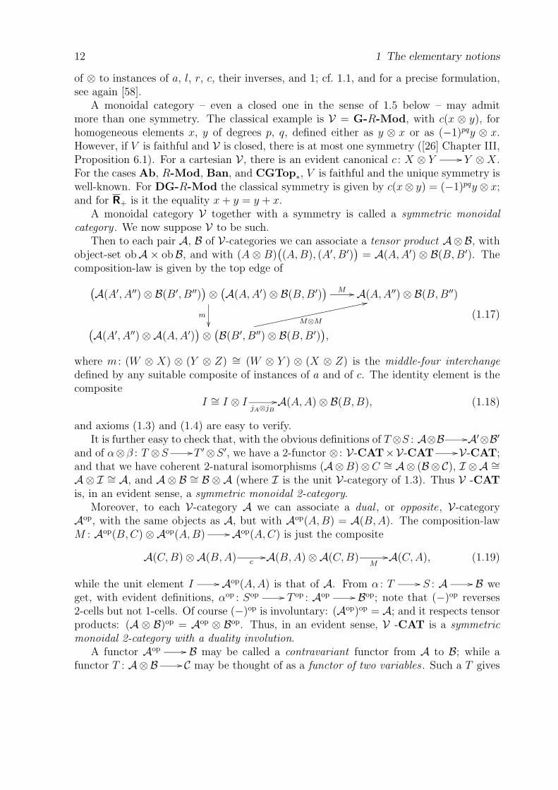
A monoidal category – even a closed one in the sense of 1.5 below – may admitmore than one symmetry. The classical example is V = G-R-Mod, with c(x ⊗ y), forhomogeneous elements x, y of degrees p, q, defined either as y ⊗ x or as (−1)pqy ⊗ x.However, if V is faithful and V is closed, there is at most one symmetry ([26] Chapter III,Proposition 6.1). For a cartesian V , there is an evident canonical c : X ⊗ Y Y ⊗ X.For the cases Ab, R-Mod, Ban, and CGTop∗, V is faithful and the unique symmetry iswell-known. For DG-R-Mod the classical symmetry is given by c(x⊗ y) = (−1)pqy ⊗ x;and for R+ is it the equality x + y = y + x.
A monoidal category V together with a symmetry is called a symmetric monoidalcategory . We now suppose V to be such.
Then to each pair A, B of V-categories we can associate a tensor product A⊗B, withobject-set obA × obB, and with (A ⊗ B)
((A,B), (A′, B′)
)= A(A,A′) ⊗ B(B,B′). The
composition-law is given by the top edge of
(A(A′, A′′) ⊗ B(B′, B′′)
)⊗
(A(A,A′) ⊗ B(B,B′)
) M
m
A(A,A′′) ⊗ B(B,B′′)
(A(A′, A′′) ⊗A(A,A′)
)⊗
(B(B′, B′′) ⊗ B(B,B′)
),
M⊗M
(1.17)
where m : (W ⊗ X) ⊗ (Y ⊗ Z) ∼= (W ⊗ Y ) ⊗ (X ⊗ Z) is the middle-four interchangedefined by any suitable composite of instances of a and of c. The identity element is thecomposite
I ∼= I ⊗ IjA⊗jB
A(A,A) ⊗ B(B,B), (1.18)
and axioms (1.3) and (1.4) are easy to verify.It is further easy to check that, with the obvious definitions of T⊗S : A⊗B A′⊗B′
and of α⊗β : T ⊗S T ′⊗S ′, we have a 2-functor ⊗ : V-CAT×V-CAT V-CAT;and that we have coherent 2-natural isomorphisms (A⊗B)⊗C ∼= A⊗ (B⊗C), I ⊗A ∼=A⊗ I ∼= A, and A⊗ B ∼= B ⊗A (where I is the unit V-category of 1.3). Thus V -CATis, in an evident sense, a symmetric monoidal 2-category.
Moreover, to each V-category A we can associate a dual , or opposite, V-categoryAop, with the same objects as A, but with Aop(A,B) = A(B,A). The composition-lawM : Aop(B,C) ⊗Aop(A,B) Aop(A,C) is just the composite
A(C,B) ⊗A(B,A) cA(B,A) ⊗A(C,B)
MA(C,A), (1.19)
while the unit element I Aop(A,A) is that of A. From α : T S : A B weget, with evident definitions, αop : Sop T op : Aop Bop; note that (−)op reverses2-cells but not 1-cells. Of course (−)op is involuntary: (Aop)op = A; and it respects tensorproducts: (A ⊗ B)op = Aop ⊗ Bop. Thus, in an evident sense, V -CAT is a symmetricmonoidal 2-category with a duality involution.
A functor Aop B may be called a contravariant functor from A to B; while afunctor T : A⊗B C may be thought of as a functor of two variables. Such a T gives

1.5 Closed and biclosed monoidal categories 13
rise to partial functors T (A,−) : B C for each A ∈ A and T (−, B) : A C for eachB ∈ B. Here T (A,−) is the composite
B ∼= I ⊗ BA⊗1
A⊗ BT
C, (1.20)
from which can be read off the value of T (A,−)BB′ .Suppose, conversely, that we are given a family of functors T (A,−) : B C indexed
by obA and a family of functors T (−, B) : A C indexed by obB, such that on objectswe have T (A,−)B = T (−, B)A, = T (A,B), say. Then there is a functor T : A⊗B Cof which these are the partial functors if and only if we have commutativity in
A(A, A′) ⊗ B(B, B′)
c
T (−,B′)⊗T (A,−) C(T (A, B′), T (A′, B′)
)⊗ C
(T (A, B), T (A, B′)
)M
C(T (A, B), T (A′, B′)
)
B(B, B′) ⊗A(A, A′)T (A′,−)⊗T (−,B) C
(T (A′, B), T (A′, B′)
)⊗ C
(T (A, B), T (A′, B)
).
M
(1.21)
Moreover T is then unique, and T(A,B),(A′,B′) is the diagonal of (1.21). The verification iseasy, and the details can be found in ([26] Chapter III, S 4).
It is further easy (using (1.21), and (1.3) for C) to verify that, if T , S : A⊗B C, afamily αAB : T (A,B) S(A,B) in C0 constitutes a V-natural transformation T Sif and only if it constitutes, for each fixed A, a V-natural T (A,−) S(A,−), and, foreach fixed B, a V-natural T (−, B) S(−, B). In other words, V-naturality may beverified variable-by-variable.
In relation to the underlying ordinary categories, we have of course (Aop)0 = (A0)op
and (T op)0 = (T0)op. However, (A⊗B)0 is not A0×B0; rather there is an evident canonical
functor A0 × B0 (A ⊗ B)0, and a similar one 1 I0. For T : A ⊗ B C, the
partial functors of the composite ordinary functor
A0 × B0(A⊗ B)0 T0
C0 (1.22)
are precisely T (A,−)0 and T (−, B)0.We could discuss, in the present setting, the extraordinary V-natural families of 1.7
below. However, the techniques that make this simple arise more naturally, and at ahigher level, when V is closed; which is the case of real interest. Moreover it is shownin [17] that any symmetric monoidal category can, by passing to a higher universe, beembedded in a closed one; see also 2.6 and 3.11 below.
1.5 Closed and biclosed monoidal categories
The monoidal category V (symmetric or not) is said to be closed (cartesian closed , whenV is cartesian monoidal) if each functor − ⊗ Y : V0
V0 has a right adjoint [Y,−]; so
14 1 The elementary notions
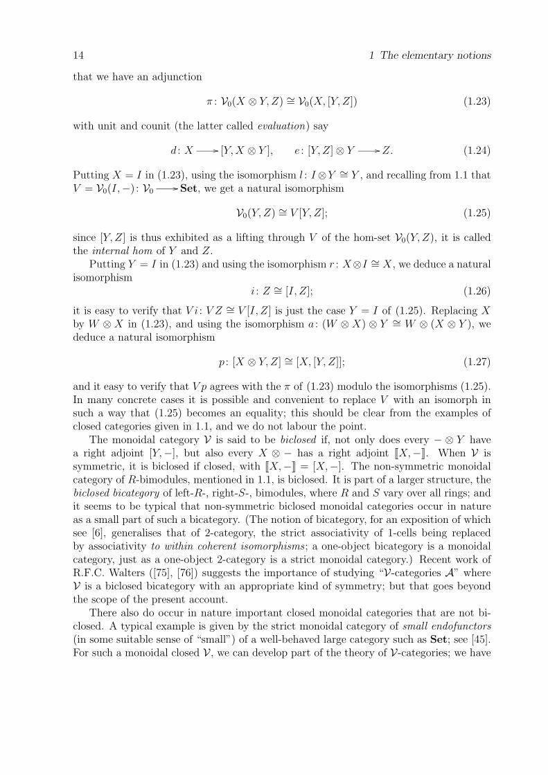
that we have an adjunction
π : V0(X ⊗ Y, Z) ∼= V0(X, [Y, Z]) (1.23)
with unit and counit (the latter called evaluation) say
d : X [Y,X ⊗ Y ], e : [Y, Z] ⊗ Y Z. (1.24)
Putting X = I in (1.23), using the isomorphism l : I ⊗Y ∼= Y , and recalling from 1.1 thatV = V0(I,−) : V0
Set, we get a natural isomorphism
V0(Y, Z) ∼= V [Y, Z]; (1.25)
since [Y, Z] is thus exhibited as a lifting through V of the hom-set V0(Y, Z), it is calledthe internal hom of Y and Z.
Putting Y = I in (1.23) and using the isomorphism r : X⊗I ∼= X, we deduce a naturalisomorphism
i : Z ∼= [I, Z]; (1.26)
it is easy to verify that V i : V Z ∼= V [I, Z] is just the case Y = I of (1.25). Replacing Xby W ⊗ X in (1.23), and using the isomorphism a : (W ⊗ X) ⊗ Y ∼= W ⊗ (X ⊗ Y ), wededuce a natural isomorphism
p : [X ⊗ Y, Z] ∼= [X, [Y, Z]]; (1.27)
and it easy to verify that V p agrees with the π of (1.23) modulo the isomorphisms (1.25).In many concrete cases it is possible and convenient to replace V with an isomorph insuch a way that (1.25) becomes an equality; this should be clear from the examples ofclosed categories given in 1.1, and we do not labour the point.
The monoidal category V is said to be biclosed if, not only does every − ⊗ Y havea right adjoint [Y,−], but also every X ⊗ − has a right adjoint X,−. When V issymmetric, it is biclosed if closed, with X,− = [X,−]. The non-symmetric monoidalcategory of R-bimodules, mentioned in 1.1, is biclosed. It is part of a larger structure, thebiclosed bicategory of left-R-, right-S-, bimodules, where R and S vary over all rings; andit seems to be typical that non-symmetric biclosed monoidal categories occur in natureas a small part of such a bicategory. (The notion of bicategory, for an exposition of whichsee [6], generalises that of 2-category, the strict associativity of 1-cells being replacedby associativity to within coherent isomorphisms; a one-object bicategory is a monoidalcategory, just as a one-object 2-category is a strict monoidal category.) Recent work ofR.F.C. Walters ([75], [76]) suggests the importance of studying “V-categories A” whereV is a biclosed bicategory with an appropriate kind of symmetry; but that goes beyondthe scope of the present account.
There also do occur in nature important closed monoidal categories that are not bi-closed. A typical example is given by the strict monoidal category of small endofunctors(in some suitable sense of “small”) of a well-behaved large category such as Set; see [45].For such a monoidal closed V , we can develop part of the theory of V-categories; we have

1.6 V as a V-category; representable V-functors 15
the results of 1.2 and 1.3, but not those of 1.4; and we have the Yoneda Lemma of 1.9below, but not its extra-variable form. However, we do not pursue this at all, for inpractice it seems that the interest in such a V lies in V itself, not in V-categories – whichbecome interesting chiefly when V is symmetric monoidal closed.
We end this section with two further comments on examples. First, the symmetric(cartesian) monoidal Top is not closed: −× Y cannot have a right adjoint since it doesnot preserve regular epimorphisms; see [19]. Next, to the examples of symmetric monoidalclosed category in 1.1, we add one more class. An ordered set V with finite intersectionsand finite unions is called a Heyting algebra if it is cartesian closed; a boolean algebra is aspecial case.
1.6 V as a V-category for symmetric monoidal closed V ; representableV-functors
From now on we suppose that our given V is symmetric monoidal closed, with V0 locallysmall. The structure of V -CAT then becomes rich enough to permit of Yoneda-lemmaarguments formally identical with those in CAT. Before giving the Yoneda Lemma and itsextensions in 1.9, we collect in this section and the next two some necessary preliminaries:results many of which are almost trivial in CAT, but less so here.
The proof of each assertion of these sections is the verification of the commutativityof a more-or-less large diagram. This verification can be done wholesale, in that eachdiagram involved is trivially checked to be of the type proved commutative in the coher-ence theorems of [47] and [48]. Yet direct verifications, although somewhat tedious, arenevertheless fairly straightforward if the order below is followed.
The first point is that the internal-hom of V “makes V itself into a V-category”. Moreprecisely, there is a V-category, which we call V , whose objects are those of V0, andwhose hom-object V(X,Y ) is [X,Y ]. Its composition-law M : [Y, Z] ⊗ [X,Y ] [X,Z]corresponds under the adjunction (1.23) to the composite
([Y, Z] ⊗ [X,Y ]) ⊗ X a [Y, Z] ⊗ ([X,Y ] ⊗ X)
1⊗e [Y, Z] ⊗ Y e
Z, (1.28)
and its identity element jX : I [X,X] corresponds under (1.23) to l : I ⊗ X X.Verification of the axioms (1.3) and (1.4) is easy when we recall that, because of therelation of e to the π of (1.23), the definition (1.28) of M is equivalent to e(M ⊗ 1) =e(1 ⊗ e)a. It is further easily verified that (1.25) gives an isomorphism between V0 andthe underlying ordinary category of the V-category V ; we henceforth identify these twoordinary categories by this isomorphism, thus rendering the notation V0 consistent withthe notation A0 of 1.3.
Next we observe that, for each V-category A and each object A ∈ A, we have therepresentable V-functor A(A,−) : A V sending B ∈ A to A(A,B) ∈ V, and with
A(A,−)BC : A(B,C) [A(A,B),A(A,C)] (1.29)
corresponding under the adjunction (1.23) to M : A(B,C) ⊗A(A,B) A(A,C). Ax-ioms (1.5) and (1.6) for a V-functor reduce easily to (1.3) and half of (1.4).

16 1 The elementary notions
Replacing A by Aop gives the contravariant representable functor A(−, B) : Aop V .The families A(A,−) and A(−, B) are the partial functors of a functor HomA : Aop ⊗A V sending (A,B) to A(A,B); for the condition (1.21) again reduces easily to (1.3)for A.
We write homA : Aop0 ×A0
V0 for the ordinary functor
Aop0 ×A0
(Aop ⊗A)0(HomA)0
V0; (1.30)
it sends (A,B) to A(A,B), and for its value on maps we write
A(f, g) : A(A,B) A(A′, B′),
where f : A′ A and g : B B′. By 1.4, the partial functors of homA are thefunctors underlying A(A,−) and A(−, B), so that our writing their values on morphismsas A(A, g) and A(f,B) is consistent with (1.12). Combining (1.11) with the definition(1.29) of A(A,−)BC , we see that A(A, g) : A(A,B) A(A,C) is the composite
A(A,B)l−1
I ⊗A(A,B)g⊗1
A(B,C) ⊗A(A,B)M
A(A,C), (1.31)
while A(f,B) : A(D,B) A(A,B) is
A(D,B)r−1
A(D,B) ⊗ I1⊗f
A(D,B) ⊗A(A,D)M
A(A,B). (1.32)
From these it follows easily that we have commutativity in
Aop0 ×A0
homA
HomA0
V0
V
Set.
(1.33)
When A = V , we see at once that homV is just the functor [−,−] : Vop0 × V0
V0.Now we observe that there is also a V-functor Ten: V ⊗ V V , sending
(X,Y ) Ten(X,Y ) = X ⊗ Y,
and with Ten(X,Y ),(X′,Y ′) : [X,X ′] ⊗ [Y, Y ′] [X ⊗ Y,X ′ ⊗ Y ′] corresponding under theadjunction (1.23) to the composite
([X,X ′] ⊗ [Y, Y ′]) ⊗ (X ⊗ Y ) m([X,X ′] ⊗ X) ⊗ ([Y, Y ′] ⊗ Y )
e⊗eX ′ ⊗ Y ′; (1.34)
when we observe that (1.34) is equivalent to e(Ten⊗1) = (e ⊗ e)m, verification of theV-functor axioms (1.5) and (1.6) is easy. The ordinary functor
V0 × V0(V ⊗ V)0 Ten0
V0 (1.35)

1.7 Extraordinary V-naturality 17
is at once seen to be ⊗ : V0×V0V0; so that, by (1.4), the underlying ordinary functor
of Ten(X,−) is X ⊗−.
For any V-categories A and B we have a commutative diagram
(Aop ⊗ Bop) ⊗ (A⊗ B)HomA⊗B
∼=
V
(Aop ⊗A) ⊗ (Bop ⊗ B)HomA ⊗HomB
V ⊗ V;
Ten
(1.36)
in terms of the partial functors, this asserts the commutativity of
A⊗ B (A⊗B)((A,B),−)
A(A,−)⊗B(B,−)
V
V ⊗ V,
Ten
(1.37)
which is easily checked. At the level of the underlying functors hom, this gives
(A ⊗ B)((f, g), (f ′, g′)
)= A(f, f ′) ⊗ B(g, g′). (1.38)
1.7 Extraordinary V-naturality
The point to be made in the next section is that all the families of maps canonically associ-ated to V , or to a V-category A, or to a V-functor T , or to a V-natural α, such as a : (X⊗Y )⊗Z X⊗ (Y ⊗Z), or e : [Y, Z]⊗Y Z, or M : A(B,C)⊗A(A,B) A(A,C),or T : A(A,B) B(TA, TB), or α : I B(TA, SA), are themselves V-natural in everyvariable. To deal with a variable like B in the case of M , we must now introduce thenotion of extraordinary V-naturality ; which later plays an essential role in the definitionof V-functor-category.
First we observe that the formulae (1.31) and (1.32) allow us to write the “ordinary”V-naturality condition (1.7) in the more compact form
A(A,B) T
S
B(TA, TB)
B(1,αB)
B(SA, SB) B(αA,1)
B(TA, SB).
(1.39)

18 1 The elementary notions
By (extraordinary) V-naturality for an obA-indexed family of maps βA : K T (A,A)in B0, where K ∈ B and T : Aop ⊗A B, we mean the commutativity of each diagram
A(A,B)T (A,−)
T (−,B)
B(T (A,A), T (A,B)
)B(βA,1)
B
(T (B,B), T (A,B)
)B(βB ,1)
B(K,T (A,B)
).
(1.40)
Duality gives the notion, for the same T and K, of a V-natural family γA : T (A,A) K;namely the commutativity of
A(A,B)T (B,−)
T (−,A)
B(T (B,A), T (B,B)
)B(1,γB)
B
(T (B,A), T (A,A)
)B(1,γA)
B(T (B,A), K
).
(1.41)
Such extraordinary V-naturality is of course fully alive in the case V = Set; it is exhibitedthere, for instance, by the “naturality in Y ” of the d and the e of (1.24). In the caseV = Set, (1.40) and (1.41) have more elementary forms obtained by evaluating themat an arbitrary f ∈ A(A,B). Clearly extraordinary V-naturality implies extraordinarySet-naturality: we only have to apply V to (1.40) and (1.41).
Just as for ordinary V-naturality, it is clear that if βA : K T (A,A) is V-natural as above, and if P : D A and Q : B C, then the maps QβPD(=Q0βPD) : QK QT (PD,PD) constitute a V-natural family QβP .
If T : (A⊗D)op ⊗ (A⊗D) B, a family βAD : K T (A,D,A,D) is V-natural in(A,D) if and only if it is V-natural in A for each fixed D and in D for each fixed A, withrespect to the partial functors T (−, D,−, D) and T (A,−, A,−) respectively. The mostdirect proof involves translating (1.40) via (1.32) into a form analogous to (1.7); then, asin the proof for ordinary V-natural transformations, it is a matter of combining (1.21)with (1.3) for C. Thus here, too, V-naturality can be verified variable-by-variable.
That being so, we can combine ordinary and extraordinary V-naturality, and speak ofa V-natural family αABC : T (A,B,B) S(A,C,C), where T : A⊗Bop ⊗B D andS : A⊗Cop ⊗C D. If each of A, B and C stands for a finite number of variables, thisis then the most general form.
The analogue of “vertical composition” for such families is the calculus of [25]. Thereare three basic cases of composability, in addition to that for ordinary V-natural transfor-mations; and two of these three are dual. Each of the three, however, is in fact a sequenceof sub-cases indexed by the natural numbers. The reader will see the pattern if we justgive the first two sub-cases of the only two essentially-different sequences; the proofs areeasy using (1.39)–(1.41).
1.8 The V-naturality of the canonical maps 19
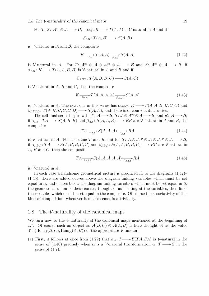
For T , S : Aop ⊗A B, if αA : K T (A,A) is V-natural in A and if
βAB : T (A,B) S(A,B)
is V-natural in A and B, the composite
K αA
T (A,A)βAA
S(A,A) (1.42)
is V-natural in A. For T : Aop ⊗ A ⊗ Aop ⊗ A B and S : Aop ⊗ A B, ifαAB : K T (A,A,B,B) is V-natural in A and B and if
βABC : T (A,B,B,C) S(A,C)
is V-natural in A, B and C, then the composite
K αAA
T (A,A,A,A)βAAA
S(A,A) (1.43)
is V-natural in A. The next one in this series has αABC : K T (A,A,B,B,C,C) andβABCD : T (A,B,B,C,C,D) S(A,D); and there is of course a dual series.
The self-dual series begins with T : A B, S : A⊗Aop⊗A B, and R : A B;if αAB : TA S(A,B,B) and βAB : S(A,A,B) RB are V-natural in A and B, thecomposite
TA αAA
S(A,A,A)βAA
RA (1.44)
is V-natural in A. For the same T and R, but for S : A ⊗ Aop ⊗ A ⊗ Aop ⊗ A B,if αABC : TA S(A,B,B,C,C) and βABC : S(A,A,B,B,C) RC are V-natural inA, B and C, then the composite
TA αAAA
S(A,A,A,A,A)βAAA
RA (1.45)
is V-natural in A.In each case a handsome geometrical picture is produced if, to the diagrams (1.42)–
(1.45), there are added curves above the diagram linking variables which must be setequal in α, and curves below the diagram linking variables which must be set equal in β;the geometrical union of these curves, thought of as meeting at the variables, then linksthe variables which must be set equal in the composite. Of course the associativity of thiskind of composition, whenever it makes sense, is a triviality.
1.8 The V-naturality of the canonical maps
We turn now to the V-naturality of the canonical maps mentioned at the beginning of1.7. Of course such an object as A(B,C) ⊗ A(A,B) is here thought of as the valueTen(HomA(B,C), HomA(A,B)) of the appropriate V-functor.
(a) First, it follows at once from (1.29) that αA : I B(TA, SA) is V-natural in thesense of (1.40) precisely when α is a V-natural transformation α : T S in thesense of (1.7).

20 1 The elementary notions
(b) Next, for a V-functor T : A B, the map TAB : A(A,B) B(TA, TB) is V-natural in both variables A and B. It suffices to verify V-naturality in B; and herethe appropriate diagram of the form (1.39) reduces, in the light of (1.29), to (1.5) forT .
(c) This last gives, for a V-functor T : A ⊗ B C, the V-naturality in A and A′ ofT (−, B) : A(A,A′) C(T (A,B), T (A′, B)). However, this is also V-natural in B;the appropriate instance of (1.40) reduces via (1.29) to (1.21).
(d) In particular, for a V-category A, the A(A,−)BC : A(B,C) [A(A,B),A(A,C)]of (1.29) is V-natural in all variables.
(e) Composing the A(A,−)BC of (d) with g : I A(B,C) gives, by (a), the V-naturalityin A of A(A, g) : A(A,B) A(A,C).
(f) The V-naturality in both variables of e : [Y, Z] ⊗ Y Z is an easy consequence of(1.29) and (1.34).
(g) Since, by (1.29), M : A(B,C) ⊗ A(A,B) A(A,C) for a V-category A is thecomposite
A(B,C) ⊗A(A,B) A(A,−)⊗1 [A(A,B),A(A,C)] ⊗A(A,B) e
A(A,C),
it is V-natural in all variables by (d), (e), (f), (1.42) and (1.44).
(h) The V-naturality of jA : I A(A,A) for a V-category A follows from (a), since1 : 1 1: A A is V-natural.
(i) The V-naturality in every variable of a : (X⊗Y )⊗Z X⊗(Y ⊗Z), l : I⊗X X,r : X ⊗ I X, c : X ⊗ Y Y ⊗ X, follows easily from (1.34).
(j) From the definition (1.27) of the isomorphism p and the definition (1.34) of Ten(−, Y ),we easily see that p−1 : [X, [Y, Z]] [X ⊗ Y, Z] is the composite
[X, [Y, Z]]Ten(−,Y )
[X ⊗ Y, [Y, Z] ⊗ Y ][1,e]
[X ⊗ Y, Z].
It follows from (c), (e), (f), and (1.44) that p−1 is V-natural in all variables; whencethe same is true of its inverse p.
(k) The composite
Xl−1
I ⊗ Xj⊗1
[X ⊗ Y,X ⊗ Y ] ⊗ Xp⊗1
[X, [Y,X ⊗ Y ]] ⊗ X e [Y,X ⊗ Y ]
is easily verified to be the d : X [Y,X ⊗ Y ] of (1.24); the latter is thereforeV-natural in every variable by (i), (h), (j), (f), (e), (1.42), and (1.44).
1.9 The (weak) Yoneda lemma for V -CAT 21
(l) The compositeX
d [I,X ⊗ I]
[1,r] [I,X]
is the isomorphism i : X [I,X], which is therefore V-natural.
This completes the list of canonical maps, and we end this section with a generalprinciple. Since a map f : X ⊗ Y Z and its image f : X [Y, Z] under the πof (1.23) are related by f = [1, f ]d and f = e(f ⊗ 1), it follows from (f), (k), (e) and(1.42)–(1.44) that, for V-functors T ,S,R of suitable variances with codomain V , we have:
(m) A family f : T (D,D,A,B) ⊗ S(E,E,A,C) R(F, F,B,C) is V-natural in any ofits variables if and only if the corresponding
f : T (D,D,A,B) [S(E,E,A,C), R(F, F,B,C)]
is so.
1.9 The (weak) Yoneda lemma for V -CAT
The form of the Yoneda Lemma we give here is a weak one, in that it asserts a bijectionof sets rather than an isomorphism of objects of V ; a stronger form will be given in 2.4below.
Consider a V-functor F : A V and an object K of A. To each V-natural transfor-mation α : A(K,−) F we can assign the element η : I FK of FK given by thecomposite
IjK
A(K,K) αK
FK. (1.46)
The Yoneda Lemma asserts that this gives a bijection between the set V-nat(A(K,−), F )of V-natural transformations and the set V0(I, FK) (= V FK) of elements of FK; thecomponent αA being given in terms of η as the composite
A(K,A)FKA
[FK,FA][η,1]
[I, FA]i−1
FA. (1.47)
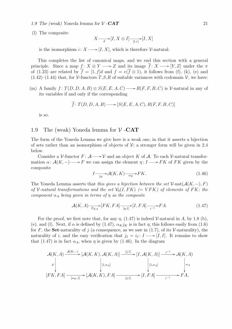
For the proof, we first note that, for any η, (1.47) is indeed V-natural in A, by 1.8 (b),(e), and (l). Next, if α is defined by (1.47), αKjK is in fact η; this follows easily from (1.6)for F , the Set-naturality of j (a consequence, as we saw in (1.7), of its V-naturality), thenaturality of i, and the easy verification that jI = iI : I [I, I]. It remains to showthat (1.47) is in fact αA, when η is given by (1.46). In the diagram
A(K,A)A(K,−)
F
[A(K,K),A(K,A)][j,1]
[1,αA]
[I,A(K,A)]i−1
[1,αA]
A(K,A)
αA
[FK,FA]
[αK ,1] [A(K,K), FA]
[j,1] [I, FA]
i−1 FA,
22 1 The elementary notions
the left square commutes by the V-naturality of α in the form (1.39), the middle squaretrivially, and the right square by the naturality of i. The proof is complete when weobserve that the top edge of the diagram is the identity; which follows from the definition(1.29) of A(K,−), the axiom (1.4) for A, and the definition (1.26) of i in terms of r.
There is an extra-variable form of the result, involving functors F : Bop ⊗ A Vand K : B A, and a family αBA : A(KB,A) F (B,A) which is V-natural in A foreach fixed B, so that it corresponds as above to a family ηB : I F (B,KB). It thenfollows from (1.46) and (1.42) that η is V-natural in B if α is, and from (1.47) and (1.44)that α is V-natural in B if η is.
It is worth noting an alternative way of writing (1.47) when F has the form B(B, T−)for a V-functor T : A B, so that η : I B(B, TK) is then a map η : B TKin B0 (in fact, the image of 1K under V αK : A0(K,K) B0(B, TK)). Then αA is thecomposite
A(K,A)TKA
B(TK, TA) B(η,1)B(B, TA), (1.48)
which is easily seen by (1.32) to coincide with (1.47). In particular, every V-naturalα : A(K,−) A(L,−) is A(k,−) for a unique k : L K; and clearly k is an iso-morphism if and only if α is.
1.10 Representability of V-functors; the representing object as a V-functor of the passive variables
We have called the V-functors A(K,−) : A V representable. More generally, however,a V-functor F : A V is called representable if there is some K ∈ A and an isomorphismα : A(K,−) F . Then the pair (K,α) is a representation of F ; it is essentially uniqueif it exists, in the sense that any other representation α′ : A(K ′,−) F has the formα′ = α.A(k,−) for a unique isomorphism k : K K ′. The corresponding η : I FKis called the unit of the representation. (We call η the counit when we are representing acontravariant F : Aop V in the form A(−, K).)
For a general V , there is no simple criterion in terms of an η : I FK for thecorresponding α : A(K,−) F to be an isomorphism. It is of course otherwise in theclassical case V = Set; there we have the comma-category 1/F = el F of “elements of F”,whose objects are pairs (A, x) with A ∈ A and x ∈ FA; and α is invertible if and only if(K, η) is initial in el F , so that F is representable if and only if el F has an initial object.However, any such kind of “universal property” criterion ultimately expresses a bijectionof sets, and cannot suffice in general to characterize an isomorphism in V0.
Now let F : Bop ⊗ A V be such that each F (B,−) : A V admits a rep-resentation αB : A(KB,−) F (B,−). Then there is exactly one way of definingKBC : B(B,C) A(KB,KC) that makes K a V-functor for which
αBA : A(KB,A) F (B,A)
is V-natural in B as well as A.
1.11 Adjunctions and equivalences in V -CAT 23
For by 1.9, the V-naturality in B of αBA is equivalent to that of ηB, which by (1.40)means the commutativity of
B(B,C)KBC
F (−,KC)
A(KB,KC)F (B,−) [F (B,KB), F (B,KC)]
[ηB ,1]
[F (C,KC), F (B,KC)]
[ηC ,1] [I, F (B,KC)].
(1.49)
Now the composite [ηB, 1]F (B,−) in this diagram is, by (1.47), the composite isomor-phism
A(KB,KC) αB,KC
F (B,KC)i
[I, F (B,KC)];
so that (1.49) forces us to define KBC as
KBC = α−1i−1[ηC , 1]F (−, KC). (1.50)
This composite (1.50) is V-natural in B, by 1.7 and 1.8; and from this the proof of 1.8(b),read backwards, gives the V-functor axiom (1.5) for K; while the remaining V-functoraxiom (1.6) is a trivial consequence of (1.49).
1.11 Adjunctions and equivalences in V -CAT
As in any 2-category (see [49]) an adjunction η, ε : S T : A B in V -CAT betweenT : A B (the right adjoint) and S : B A (the left adjoint) consists of η : 1 TS(the unit) and ε : ST 1 (the counit) satisfying the triangular equations Tε.ηT = 1 andεS.Sη = 1. By the Yoneda Lemma of 1.9, such adjunctions in V -CAT are in bijectionwith V-natural isomorphisms
n : A(SB,A) ∼= B(B, TA); (1.51)
for by (1.48) a V-natural map n : A(SB,A) B(B, TA) has the form n = B(η, 1)T fora unique η, while a V-natural map n : B(B, TA) A(SB,A) has the form n = A(1, ε)Sfor a unique ε, and the equations nn = 1 and nn = 1 reduce by Yoneda precisely to thetriangular equations.
The 2-functor (−)0 : V-CAT CAT carries such an adjunction into an ordinaryadjunction η, ε : S0 T0 : A0
B0 in CAT. It is immediate from (1.33) that thecorresponding isomorphism of hom-sets is
V n : A0(SB,A) ∼= B0(B, TA). (1.52)
Note that the unit and counit of this ordinary adjunction are the same η and ε, now seenas natural rather than V-natural.
By 1.10, a V-functor T : A B has a left adjoint (which is then unique to withinisomorphism, as in any 2-category) exactly when each B(B, T−) is representable. More

24 1 The elementary notions
generally, if those B for which B(B, T−) is representable constitute the full subcategoryB′ of B, we get a V-functor S : B′ A called a partial left adjoint to T .
When V is conservative – faithfulness is not enough – the existence of a left adjointS0 for T0 implies that of a left adjoint S for T : we set SB = S0B, define a map n thatis V-natural in A by n = B(η, 1)T as above (using the unit η for S0 T0), and deducethat n is an isomorphism since the V n of (1.52) is. Thus, taking V = Ab for instance,an additive functor has a left adjoint exactly when its underlying functor has one.
Again by 1.10, in the extra-variable case of a V-functor T : Cop ⊗ A B, if eachT (C,−) has a left adjoint S(−, C), then S automatically becomes a V-functor B⊗C Ain such a way that n : A(S(B,C), A) ∼= B(B, T (C,A)) is V-natural in all three variables.An evident example, with A = B = C = V , is the adjunction p : [X ⊗ Y, Z] ∼= [X, [Y, Z]]of (1.27).
For a typical adjunction (1.51) as above, we have a commutative diagram
A(A,A′)
A(ε,1)
TAA′ B(TA, TA′)
A(STA,A′);
n
(1.53)
this follows from Yoneda on setting A′ = A and composing both legs with j, since(V n)(εA) = 1. Because n is an isomorphism, we conclude that T is fully faithful ifand only if ε is an isomorphism. In consequence, a right adjoint T is fully faithful exactlywhen T0 is so.
As in any 2-category, a V-functor T : A B is called an equivalence, and wewrite T : A B, if there is some S : B A and isomorphisms η : 1 ∼= TS andρ : ST ∼= 1. Replacing ρ (still in any 2-category) by the isomorphism ε : ST ∼= 1 given byε = ρ.Sη−1T.ρ−1ST , we actually have an adjunction η, ε : S T : A B. The word“equivalence” is sometimes used to mean an adjunction in which, as here η and ε areisomorphisms; we write S T : A B.
In the 2-category V -CAT, T : A B is an equivalence if and only if T is fully faithfuland essentially surjective on objects ; the latter means that every B ∈ B is isomorphic (inB0, of course) to TA for some A ∈ A; we often omit the words “on objects”.
For, if T is an equivalence, T is fully faithful since ε is an isomorphism, and is essentiallysurjective on objects since ηB : B TSB is an isomorphism. As for the converse,we choose for each B ∈ B an SB ∈ A and an isomorphism ηB : B TSB. Thecorresponding V-natural-in-A transformation n = B(ηB, 1)T : A(SB,A) B(B, TA) isthen an isomorphism because T is fully faithful, so that S becomes automatically a V-functor left adjoint to T . Since η is an isomorphism, so is Tε, by the triangular equationTε.ηT = 1; whence ε is an isomorphism by (1.12), since a fully-faithful T0 is certainlyconservative.
In any 2-category (see [49]) adjunctions can be composed, forming a category, ofwhich the equivalences are a subcategory. It follows from Yoneda that the composition ofadjunctions in V -CAT corresponds to the composition of the V-natural isomorphisms in
A(SS ′B,A) ∼= B(S ′B, TA) ∼= B(B, T ′TA). (1.54)

1.11 Adjunctions and equivalences in V -CAT 25
It is further true in any 2-category (see [49]) that, given adjunctions η, ε : S T : A B and η′, ε′ : S ′ T ′ : A′ B′ and 1-cells P : A A′ and Q : B B′,there is a bijection (with appropriate naturality properties) between 2-cells λ : QT T ′Pand 2-cells µ : S ′Q PS. In V -CAT it follows from Yoneda that λ and µ determineone another through the commutativity of
A(SB,A)
P
n∼=
B(B, TA)
Q
A′(PSB, PA)
A′(µ,1)
B′(QB,QTA)
B′(1,λ)
A′(S ′QB,PA)
n′∼= B′(QB, T ′PA);
(1.55)
such a pair λ, µ may be called mates .In particular, when A′ = A with P = 1 and B′ = B with Q = 1, so that S T and
S ′ T ′ are both adjunctions A B, we have a bijection between the λ : T T ′
and the µ : S ′ S. The adjunctions become a 2-category when we define a 2-cell fromS T to S ′ T ′ to be such a pair (λ, µ).
Any T : A B determines two full subcategories of B; the full image A′ of T ,determined by those B of the form TA, and the replete image A′′ of T , determined bythose B isomorphic to some TA. Clearly A′ and A′′ are equivalent; and each is equivalentto A if T is fully faithful. A full subcategory which contains all the isomorphs of itsobjects is said to be replete; any full subcategory has a repletion, namely the repleteimage of its inclusion. Clearly a fully-faithful T : A B has a left adjoint if and onlyif the inclusion A′ B has one, and if and only if the inclusion A′′ B has one.
A full subcategory A of B is called reflective if the inclusion T : A B has a leftadjoint. This implies, of course, that A0 is reflective in B0, but is in general strictlystronger. It follows – since it is trivially true for ordinary categories – that every retract(in B0) of an object of the reflective A lies in the repletion of A.
When A is reflective we may so choose the left adjoint S : B A that ε : ST 1is the identity. Then η : 1 R = TS : B B satisfies R2 = R, ηR = Rη = 1. Such an(R, η) is called an idempotent monad on B. Conversely, for any idempotent monad (R, η),both its full image and its replete image are reflective in B. If R is formed as above, thefull image is A again; but (R, η) is not uniquely determined by A. The replete image ofR is the repletion of A; and there is an evident bijection between full replete reflectivesubcategories of B and isomorphism classes of idempotent monads on B.

26 1 The elementary notions

Chapter 2
Functor categories
2.1 Ends in VSo far we have supposed that V is symmetric monoidal closed, and that the underlyingordinary category V0 is locally small. Henceforth we add the assumption that V0 iscomplete, in the sense that it admits all small limits; and from 2.5 on, we shall supposeas well that V0 is cocomplete.
Consider a V-functor T : Aop ⊗A V . If there exists a universal V-natural familyλA : K T (A,A), in the sense that every V-natural αA : X T (A,A) is given byαA = λAf for a unique f : X K, we call (K,λ) the end of T ; it is clearly unique towithin a unique isomorphism when it exists. We write
∫A∈A T (A,A) for the object K,
and by the usual abuse of language also call this object the end of T : then the universalV-natural λA :
∫A
T (A,A) T (A,A) may be called the counit of this end.The V-naturality condition (1.40), in the case B = V , transforms under the adjunction
V0(X, [Y, Z]) ∼= V0(X ⊗ Y, Z) ∼= V0(Y, [X,Z]) into
KλA
λB
T (A,A)
ρAB
T (B,B) σAB
[A(A,B), T (A,B)],
(2.1)
where ρAB and σAB are the transforms of T (A,−)AB and T (−, B)BA. It follows that,when A is small, the end
∫A∈A T (A,A) certainly exists, and is given as an equalizer
∫A∈A T (A,A)
λ∏
A∈A T (A,A)ρ σ
∏
A,B∈A[A(A,B), T (A,B)]. (2.2)
If A, while not necessarily small, is equivalent to a small V-category, then the fullimage in A of the latter is a small full subcategory A′ for which the inclusion A′ A isan equivalence. Since it clearly suffices to impose (2.1) only for A, B ∈ A′, it follows that∫
A∈A T (A,A) still exists, being∫
A∈A′ T (A,A). In consequence, we henceforth change themeaning of “small”, extending it to include those V-categories equivalent to small ones inthe sense of 1.2.
27
28 2 Functor categories
The universal property of the end – expressed, as it stands, by a bijection of sets – infact lifts to an isomorphism in V0; in the sense that
[X,λA] : [X,∫
AT (A,A)] [X,T (A,A)]
expresses its domain as the end of its codomain:
[X,∫
AT (A,A)] ∼=
∫A[X,T (A,A)] (with counit [X,λA]). (2.3)
For Y [X,T (A,A)] is V-natural if and only if Y ⊗X T (A,A) is, by 1.8(m). Notethat the right side of (2.3) exists for all X if
∫A
T (A,A) exists; the converse of this is alsotrue, as we see on taking X = I.
If α : T T ′ : Aop ⊗A V , and if the ends of T and T ′ exist, the top leg of thediagram ∫
AT (A,A)
λA
∫A αAA
T (A,A)
αAA
∫A
T ′(A,A)λ′
A
T ′(A,A)
(2.4)
is V-natural by (1.42); so that, by the universal property of λ′, there is a unique∫
AαAA
rendering the diagram commutative.This “functoriality” of ends lifts, in the appropriate circumstances, to a V-functoriality.
Suppose namely that, for T : Aop ⊗A⊗B V , the end HB =∫
AT (A,A,B) exists for
each B. Then there is exactly one way of making H into a V-functor H : B V thatrenders λAB : HB T (A,A,B) V-natural in B as well as in A.
For, by (1.39), the V-naturality in B is expressed by the commutativity of
B(B,C)HBC
T (A,A,−)
[HB,HC]
[1,λAC ]
[T (A,A,B), T (A,A,C)]
[λAB ,1] [HB, T (A,A,C)].
(2.5)
The bottom leg is V-natural in A by 1.8(c), 1.8(e), and (1.43). The right edge is itselfan end by (2.3). Hence a unique HBC renders the diagram commutative. The V-functoraxioms (1.5) and (1.6) for H then follow from the V-naturality of M and j (1.8(g) and(h)), the composition-calculus of 1.7, and the universal property of the counit [1, λ].
In these circumstances, if R : B V , a family βB : RB ∫
AT (A,A,B) is V-natural
in B if and only if the composite
RBβB
∫
AT (A,A,B)
λAB
T (A,A,B) (2.6)
is so. One direction is trivial, while the other follows easily from (2.5) and the universalproperty of the counit [1, λ]. In fact, this result can also be seen – using 1.8(m) to view

2.2 The functor-category [A,B] for small A 29
(2.6) as a V-natural family I [RB, T (A,A,B)] and using (2.3) – as a special case ofthe following.
Let T : (A ⊗ B)op ⊗ (A ⊗ B) V , recalling that (A ⊗ B)op = Aop ⊗ Bop. Supposethat, for each B, C ∈ B, the end
∫A∈A T (A,B,A,C) exists; then, as above, it is the value
of a V-functor Bop ⊗B V . Every family αAB : X T (A,B,A,B) that is V-naturalin A factorizes uniquely as
XβB
∫
A∈A T (A,B,A,B)λABB
T (A,B,A,B); (2.7)
and it follows again from (2.5) and the universal property of [1, λ] that the V-naturalityin B of αAB is equivalent to the V-naturality in B of βB.
Since, by 1.7, V-naturality of αAB in A and B separately coincides with its V-naturalityin (A,B) ∈ A⊗ B, we deduce the Fubini Theorem: if every
∫A
T (A,B,A,C) exists, then∫(A,B)∈A⊗B T (A,B,A,B) ∼=
∫B∈B
∫A∈A T (A,B,A,B), (2.8)
either side existing if the other does.This in turn gives, since A⊗B ∼= B⊗A, the following interchange of ends theorem, of-
ten itself called the Fubini Theorem: if every∫
AT (A,B,A,C) and every
∫B
T (A,B,D,B)exists, then ∫
A∈A∫
B∈B T (A,B,A,B) ∼=∫
B∈B∫
A∈A T (A,B,A,B), (2.9)
either side existing if the other does.
2.2 The functor-category [A,B] for small AFor V-functors T , S : A B we introduce the notation
[A,B](T, S) =∫
A∈A B(TA, SA) (2.10)
for the end on the right, whenever it exists; and we write the counit as
EA = EA,TS : [A,B](T, S) B(TA, SA). (2.11)
We write [A,B]0(T, S) for the set V [A,B](T, S) of elements α : I [A,B](T, S) of thisend. These of course correspond to V-natural families
αA = EAα : I B(TA, SA), (2.12)
which by 1.8(a) are precisely the V-natural transformations α : T S : A B.Note that, by (2.3) and the adjunction [X, [Y, Z]] ∼= [Y, [X,Z]], we have
[X, [A,V ](T, S)] ∼= [A,V ](T, [X,S−]), (2.13)
either side existing for all X ∈ V if the other does.When [A,B](T, S) exists for all T , S : A B, as it surely does by 2.1 if A is
small, it is the hom-object of a V-category [A,B] with all the T : A B as objects.

30 2 Functor categories
The composition law of [A,B] is, by 1.8(g), (1.43), and the universal property of EA,TR,uniquely determined by the commutativity of
[A,B](S,R) ⊗ [A,B](T, S) M
EA⊗EA
[A,B](T,R)
EA
B(SA,RA) ⊗ B(TA, SA)
M B(TA,RA),
(2.14)
and its identity elements are similarly determined by
EAjT = jTA; (2.15)
the axioms (1.3) and (1.4) follow at once from the corresponding axioms for B and theuniversal property of EA.
We call [A,B] the functor category ; its underlying category [A,B]0 is by (2.12) theordinary category of all V-functors A B and all V-natural transformations betweenthem – that is
[A,B]0 = V-CAT(A,B). (2.16)
Even when [A,B] does not exist, it may sometimes be convenient to use [A,B]0 as anabbreviation for V-CAT(A,B).
When [A,B] exists, the function T → TA and the maps EA,TS of (2.11) constitute,by (2.14) and (2.15), a V-functor EA : [A,B] B, called evaluation at A. By (2.12),the ordinary functor underlying EA sends a map α ∈ [A,B]0(T, S) to its component αA.
There is a V-functor E : [A,B] ⊗ A B, simply called evaluation, whose partialfunctors are given by
E(−, A) = EA : [A,B] B, E(T,−) = T : A B. (2.17)
To show this we must verify the appropriate instance of (1.21); but, by the proof of 1.8(c)read backwards, this instance reduces via (1.29) to the instance of (1.40) expressing theV-naturality in A of EA,TS.
More generally, [A,B](T, S) may exist, not for all T , S, but for all those in somesubset of the set of V-functors A B; a typical example would be the subset of thoseA B which are left Kan extensions, in the sense of 4.1 below, of their restrictions tosome fixed small full subcategory of A. Then we get as above a V-category [A,B]′ withthese functors as objects, whose underlying category [A,B]′0 is the corresponding fullsubcategory of V-CAT(A,B); and we have the evaluation functor E : [A,B]′ ⊗A B.
Still more generally, we may wish to consider [A,B](T, S) just for certain particularpairs T , S for which it exists – as in the Yoneda isomorphism of 2.4 below. To discuss itsfunctoriality in this generality, suppose we have functors P : C ⊗ A B and Q : D ⊗A B such that [A,B]
(P (C,−), Q(D,−)
)exists for each C and D. Then there is, by
2.1, a unique V-functor H : Cop ⊗D V having
H(C,D) = [A,B](P (C,−), Q(D,−)
), (2.18)
2.3 The isomorphism [A⊗ B, C] ∼= [A, [B, C]] 31
with respect to which EA : [A,B](P (C,−), Q(D,−)
) B
(P (C,A), Q(D,A)
)is V-
natural in C and D as well as A. Moreover by (2.6) and (2.7), in the situations (thesecond of which has D = C)
R(C,D)βCD
αACD
[A,B]
(P (C,−), Q(D,−)
)EA
B
(P (C,A), Q(D,A)
),
XβC
αAC
[A,B](P (C,−), Q(C,−)
)EA
B
(P (C,A), Q(C,A)
),
(2.19)α is V-natural in C or D if and only if β is.
When [A,B], or even some [A,B]′, exists, the H of (2.18) can be given more explicitly– see 2.3 below.
2.3 The isomorphism [A⊗ B, C] ∼= [A, [B, C]]
We return to the case where [A,B] exists. The V-functor E : [A,B] ⊗ A B induces,for each V-category C, an ordinary functor
V-CAT(C, [A,B]) V-CAT(C ⊗A,B), (2.20)
sending G : C [A,B] to the composite
C ⊗ AG⊗1
[A,B] ⊗AE
B, (2.21)
and sending β : G G′ : C [A,B] to the composite E(β ⊗ 1A). Clearly the map(2.20) is 2-natural in C; and in fact it is an isomorphism of categories.
To prove this we must first show that every P : C ⊗ A B has the form (2.21) fora unique G. Equating the partial functors of P and (2.21) gives
P (C,−) = GC, P (−, A) = EAG. (2.22)
The first of these determines G on objects, whereupon the second asserts the commuta-tivity of
C(C,D)GCD
P (−,A)CD
[A,B]
(P (C,−), P (D,−)
)EA
B
(P (C,A), P (D,A)
).
(2.23)
Since P (−, A)CD is V-natural in A by 1.8(c), this determines a unique GCD by the uni-versal property of EA. By this same universal property together with the composition-calculus of 1.7, the V-functor axioms (1.5) and (1.6) for G follow at once from those forP (−, A).

32 2 Functor categories
Before showing that (2.20) is bijective on maps as well as on objects, let us analyzethe V-functoriality (2.18) when [A,B] exists. If P : C ⊗ A B and Q : D ⊗ A Bcorrespond by (2.20) to G : C [A,B] and F : D [A,B], we have the compositeV-functor
Cop ⊗DGop⊗F
[A,B]op ⊗ [A,B]Hom[A,B]
V ; (2.24)
and with respect to this, EA : [A,B](GC,FD) B(EAGC,EAFD) is V-natural in Cand D, by 1.7 and 1.8(b). By (2.22), this EA is
EA : [A,B](P (C,−), Q(D,−)
) B
(P (C,A), Q(D,A)
);
hence the H of (2.18), by its uniqueness, must be (2.24).To complete the proof that (2.20) is an isomorphism of categories, it remains to verify
that, if P and P ′ are the images under (2.20) of G and G′, every α : P P ′ is E(β⊗1A)for a unique β : G G′. By (2.22) the equation α = E(β⊗1A) has the component-formαCA = EAβC , which by (2.12) is
αCA = EAβC = (βC)A. (2.25)
Thus βC : GC G′C must be the V-natural transformation αC− : P (C,−) P ′(C,−);and the proof will be complete when we show that βC , so defined, is V-natural in C. Ifwe look on βC as a map I [A,B](GC,G′C), this follows from 1.8(m) and (2.19), nowthat H is identified as (2.24).
More generally, if [A,B] does not exist but some full subcategory [A,B]′ does, inthe sense of 2.2, we have by the same arguments an isomorphism between the categoryV-CAT(C, [A,B]′) and the full subcategory of V-CAT(C ⊗ A,B) determined by thoseP : C ⊗A B for which each P (C,−) lies in [A,B]′; for we have the analogue of (2.24)with [A,B]′ replacing [A,B].
The 2-natural isomorphism (2.20) exhibits [A,B], when it exists, as a representingobject for the 2-functor V-CAT(−⊗A,B). It is conversely true that, if this 2-functor isrepresentable by some D, then [A,B] exists and is isomorphic to D – at least if V0 has aninitial object 0. For taking C to be I in (2.20), with [A,B] replaced by D, we identify theobjects of D with the V-functors A B; while taking C to be the V-category with twoobjects 0 and 1, with C(0, 0) = C(1, 1) = I, with C(1, 0) = 0, and with C(0, 1) an arbitraryobject X of V , we easily see that D(T, S) =
∫AB(TA, SA).
It follows from 1.10 that, so far as it exists, [A,B] is uniquely 2-functorial in A and Bin such a way that (2.20) is 2-natural in every variable; which by 1.9 is equivalent to the2-naturality in each variable of E : [A,B]⊗A B. Using this latter criterion we easilysee that, for M : A′ A and N : B B′, the V-functor [M,N ] : [A,B] [A′,B′]sends T to NTM and is determined on hom-objects by
[A,B](T, S)[M,N ]TS
EMA
[A′,B′](NTM,NSM)
E′A
B(TMA,SMA)
NTMA,SMA
B′(NTMA,NSMA);
(2.26)

2.4 The (strong) Yoneda lemma for V -CAT; the Yoneda embedding 33
while the V-natural transformation [µ, ν] : [M,N ] [M ′, N ′] is given by
[µ, ν]T = νTµ : NTM N ′TM ′. (2.27)
As for the interplay of functor categories with duality, we clearly have a 2-natural isomor-phism
[Aop,Bop] ∼= [A,B]op, (2.28)
either side existing if the other does.The 2-functor − ⊗ A : V-CAT V-CAT has a right adjoint [A,−] when [A,B]
exists for all B; and by the above, only then, if V0 has an initial object. This right adjointsurely exists when A is small, in the extended sense of 2.1; and for many V it existsonly then. For instance, a result of Freyd (see [73])1 shows that, when V = Set, A isnecessarily small if [A,V ] exists. Yet when V0 is an ordered set, as in the cases V = 2 andV = R+, [A,B] exists for every A and B.
In this sense the symmetric monoidal 2-category V-CAT is “partially closed”; whilethe symmetric monoidal 2-category V-Cat of small V-categories is actually closed.
The partial closedness is sufficient to imply the isomorphisms (1.26) and (1.27) of 1.5,which here read:
[I,B] ∼= B, [C ⊗ A,B] ∼= [C, [A,B]], (2.29)
the latter in the sense that either side exists if the other does, provided [A,B] exists –which follows alternatively from the Fubini Theorem (2.8).
2.4 The (strong) Yoneda lemma for V -CAT; the Yoneda embeddingA [Aop,V ]
We can now give a stronger version of the Yoneda Lemma of 1.9, no longer expressed bya mere bijection of sets, but by a Yoneda isomorphism in V0.
Given a V-functor F : A V and an object K of A as in 1.9, we have the mapFKA : A(K,A) [FK,FA], which is V-natural in A by 1.8(b). The transform
φA : FK [A(K,A), FA] (2.30)
of FKA under the adjunction V0(X, [Y, Z]) ∼= V0(Y, [X,Z]) is V-natural in A by 1.8(m).The stronger Yoneda Lemma is the assertion that (2.30) expresses FK as the end∫
A[A(K,A), FA], so that we have an isomorphism
φ : FK ∼= [A,V ](A(K,−), F ]. (2.31)
For the proof, consider any V-natural αA : X [A(K,A), FA]; its transformαA : A(K,A) [X,FA] under the adjunction, being V-natural in A by 1.8(m), is thecomposite
A(K,A)FKA
[FK,FA][η,1]
[X,FA]
1For a more useful citation, see Peter Freyd and Ross Street, On the size of categories, Theory andApplications of Categories 1 (1995) 174-178.http://www.tac.mta.ca/tac/volumes/1995/n9/1-09abs.html
34 2 Functor categories
for a unique η : X FK, by the Yoneda Lemma of 1.9 in the form (1.48). This isequivalent to the assertion that αA = φAη for a unique η; which completes the proof.
The image under V = V0(I,−) : V0 Set of (2.31) is a bijection
V0(I, FK) [A,V ]0(A(K,−), F ).
This sends η : I FK to φη : A(K,−) F , whose component A(K,A) FA isEAφη by (2.12), or φAη. By the definition (2.30) of φA, this is at once seen to be thecomposite (1.47). Hence the weak Yoneda Lemma of 1.9, which we have used to prove thepresent strong Yoneda Lemma, is subsumed under the latter as its underlying bijection.
The special case F = A(L,−) : A V of the present Yoneda Lemma strengthensthe last assertion of 1.9 to
A(L,K) ∼= [A,V ](A(K,−),A(L,−)
). (2.32)
Since (2.31) is true without any smallness restriction on A, its V-naturality must ingeneral be discussed (cf. 2.2) in terms of the V-functor HomA : Aop ⊗A V and someV-functor P : C ⊗ A V . We assert that
φ = φCK : P (C,K) ∼= [A,V ](A(K,−), P (C,−)
)(2.33)
is V-natural in C and K, when the right side is made V-functorial as in (2.18). Thisfollows from (2.19); for EAφ = φA : P (C,K) [A(K,A), P (C,A)] is V-natural in Cand K by 1.8(m), since A(K,A) [P (C,K), P (C,A)] is so by 1.8(b) and 1.8(c).
When [A,V ] exists, HomA : Aop ⊗A V corresponds under (2.20) to a V-functor
Y : Aop [A,V ] (2.34)
sending K toY K = A(K,−); (2.35)
being fully faithful by (2.32), Y is called the Yoneda embedding . In these circumstances theV-naturality (2.33) can be more globally expressed by taking [A,V ] for C and E : [A,V ]⊗A V for P ; the right side of (2.33) is them by (2.24) the value of the V-functor
A⊗ [A,V ]Y op⊗1
[A,V ]op ⊗ [A,V ]Hom[A,V]
V ; (2.36)
so that, with respect to this functoriality,
the Yoneda isomorphism (2.31) is V-natural in K and F . (2.37)
The extra-variable result of 1.9 also has a lifting to the present context. LetF : Bop ⊗ A V and K : B A. By (2.33) we have an isomorphism F (C,KB) ∼=[A,V ]
(A(KB,−), F (C,−)
), V-natural in C and B. The Fubini Theorem (2.8) now gives∫
BF (B,KB) ∼= [Bop ⊗A,V ]
(A(K?,−), F (?,−)
), (2.38)
either side existing if the other does.

2.5 The free V-category on a Set-category 35
2.5 The free V-category on a Set-category
We henceforth suppose, in addition to all our former assumptions on V , that the underlyingcategory V0 is cocomplete.
Then the ordinary functor V = V0(I,−) : V0Set has a left adjoint (−) ·I, sending
the set E to the coproduct E · I of E copies of I in V0. This functor sends the cartesianproduct in Set to the tensor product in V0, in that we clearly have
(E × F ) · I ∼= (E · I) ⊗ (F · I), 1 · I ∼= I. (2.39)
The 2-functor (−)0 : V-CAT CAT now has a left adjoint (−)V . The free V-category LV on the ordinary locally-small category L has the same objects as L, and hashom-objects LV(K,L) = L(K,L) · I; its composition law and its identities are inducedfrom those of L using the isomorphisms (2.39).
For the proof, we have first to verify that LV , as defined, satisfies the V-categoryaxioms (1.3) and (1.4); this is trivial from the corresponding axioms for L.
There is an evident functor ψ : L (LV)0 which is the identity on objects, and whichis defined on morphisms by the obvious map L(K,L) V0(I,L(K,L) · I). This ψ isthe unit of the 2-adjunction in question.
In fact it is easy to see that, for a V-category B and a functor T : L B0, thereis exactly one V-functor T : LV B with T 0ψ = T : on objects we have TK = TK,while TKL : L(K,L) ·I B(TK, TL) is the transform of TKL : L(K,L) B0(TK, TL)under the adjunction (−) · I V . Verification of (1.5) and (1.6) for T is easy.
Finally, if α : T S : L B0, there is a unique V-natural α : T S : LV Bwith α0ψ = α; the component αK must be αK ∈ B0(TK, SK), and again verification of(1.7) for α is easy. This completes the proof.
If L is a small category, LV is clearly a small V-category, and we can form the functorcategory [LV ,B]. Since the underlying ordinary category [LV ,B]0 of this is V-CAT(LV ,B)by (2.16), the 2-adjunction above gives
[LV ,B]0 ∼= [L,B0]. (2.40)
2.6 Universe-enlargement V ⊂ V′ in concrete cases; [A,B] as a V ’-category for large A
The possible non-existence of a V-functor category [A,B] when A is large (= non-small) issomewhat tedious, forcing us into such circumlocutions as using (2.18) instead of (2.24),or (2.33) instead of (2.37) – which then propagate themselves throughout the applicationsbelow.
Yet when V = Set, we always do have [A,B] as a category; albeit not in general aSet-category (= locally-small category) when A and B are Set-categories, unless A issmall. It can however be seen as a Set′-category, where Set′ is the category of sets insome larger universe containing obA as an element – we are taking the view that obA isalways an honest set, and supposing that every set belongs to some universe.

36 2 Functor categories
We may ask whether such a view can be imitated for a general V . Consider first thevarious examples of a symmetric monoidal closed V given in 1.1. These are of two types:either V0 is a particular ordered set, such as 2 or R+, in which case [A,B] exists for allA; or V0 consists of the small models of some theory – small sets, small categories, smallabelian groups, small differential graded R-modules, and so on. In the latter case wecan clearly consider the category V ′
0 of models in a larger Set′, which gives a symmetricmonoidal closed category V ′, in which V with its symmetric monoidal closed structureis faithfully embedded. Moreover V ′
0 admits all limits and colimits which are small byreference to Set′; and the inclusion V0
V ′0 preserves all limits and colimits that exist
in V0. (We are supposing that our original universe contains infinite sets; otherwise wedo not have the colimit-preservation above.)
Then, for V-categories A and B, we always have a V ′-category [A,B], where Set′
is taken large enough to include obA. Since V0 V ′
0 preserves limits, to say that[A,B](T, S) exists in the sense of 2.2 is precisely to say that the object [A,B](T, S) of V ′
actually lies in V ; and to say that [A,B] exists in the sense of 2.2 – that is, as a V-category– is to say that [A,B](T, S) ∈ V for all T , S.
That a similar thing is possible for a perfectly general V follows from Day [17]. Usinghis construction, one can show that there is always a suitable V ′ whose underlying ordinarycategory V ′
0 is a full reflective subcategory of [Vop0 ,Set′], into which V0 is embedded by
Yoneda. Since the monoidal structure of V ′ is defined by coends (relative to Set′), wedefer a description of it until 3.11 and 3.12 below, after these have been introduced.

Chapter 3
Indexed limits and colimits
3.1 Indexing types; limits and colimits; Yoneda isomorphisms
For a discussion of completeness, or of Kan extensions, or of density, in the context ofV-categories, ordinary limits – defined in terms of the representability of cones – do notsuffice; we need the wider notion of indexed limit . These latter fully deserve the name of“limit”, since they enjoy all the formal properties expected of a limit-notion, and includethe classical cone-type limits as a special case. When V = Set, in contrast to the situationfor a general V , an indexed limit may be expressed as an ordinary limit; yet even here, theindexed limit is a valuable concept in its own right – its meaning is scarcely clarified byits construction as an ordinary limit. Since the cone-type limits have no special positionof dominance in the general case, we go so far as to call indexed limits simply “limits”,where confusion seems unlikely.
We may think of a V-functor F : K V as an indexing type – a small one whenK is small, which will be the usual case, but not the only one. Then we may think ofa V-functor G : K B as a diagram in B of type F . For each B ∈ B, we get from Ga V-functor B(B,G−) : K V ; and we can consider the existence in V of the object[K,V ]
(F,B(B,G−)
). If this exists for all B – as it surely does when K is small – it is as
in (2.18) the value of a V-functor Bop V . If this V-functor not only exists but admitsa representation
B(B, F,G) ∼= [K,V ](F,B(B,G−)
), (3.1)
with counit sayµ : F B(F,G, G−), (3.2)
we call the representation (F,G, µ) the limit of G indexed by F . An evidently equivalentformulation not mentioning [K,V ] explicitly is the following: each component µK of µinduces by Yoneda a family
B(B, F,G) [FK,B(B,GK)] (3.3)
V-natural in B and K; and (F,G, µ) is the limit precisely when (3.3) is an end over Kfor each B. In practice, by the usual abuse of notation, we call the representing objectF,G the limit, consigning to the background the counit µ – or equivalently the choiceof the V-natural isomorphism (3.1).
37

38 3 Indexed limits and colimits
If we take the view of 2.6, that [K,V ] always exists, if not as a V-category, thenas a V ′-category for some larger V ′, we need not be concerned with the existence of[K,V ]
(F,B(B,G−)
), but only with its representability in the form (3.1) for some F,G ∈
B. If it is so representable, the right side of (3.1) in fact lies in V , since the left side does.We shall in future take this view whenever it is convenient – usually without botheringto change “V-functor” to “V ′-functor”, and so on.
Applying V to the isomorphism (3.1) gives a bijection of sets
B0(B, F,G) ∼= [K,V0](F,B(B,G−)
); (3.4)
but the requirement that (F,G, µ) induce a bijection (3.4) is, except in the special casewhen V is conservative, strictly weaker than the requirement that it induce an isomor-phism (3.1), and does not suffice to make (F,G, µ) the limit ; see 3.7 below. Howeverit does suffice to detect (F,G, µ) as the limit if the limit is known to exist ; for theright side of (3.4) admits at most one representation to within isomorphism. An elementα : F B(B,G−) of the right side of (3.4) may be called an (F,B)-cylinder over G;then the bijection (3.4) is the assertion that every such cylinder factorizes through thecounit-cylinder µ as α = B(f, 1)µ for a unique f : B F,G.
An indexed colimit in B is nothing but an indexed limit in Bop; but it is usual to replaceK by Kop in the definition, so that we still have G : K B, but now have F : Kop V .Then the colimit of G indexed by F is the representing object F G in
B(F G,B) ∼= [Kop,V ](F,B(G−, B)
), (3.5)
with unitν : F B(G−, F G). (3.6)
When B = V , we have from (2.13) and (3.1)
F,G ∼= [K,V ](F,G) for F , G : K V , (3.7)
either side existing if the other does. Hence (3.1) and (3.5) can be written
B(B, F,G) ∼= F,B(B,G−), B(F G,B) ∼= F,B(G−, B). (3.8)
Thus, just as classical limits and colimits in an ordinary category B are defined, viarepresentability, in terms of the primitive limits – sets of cones – in Set, so indexed limitsand colimits in a V-category B are defined, via representability, in terms of indexed limitsin V ; and thus ultimately, by 2.1 and 2.2, in terms of ordinary limits in V0.
Again, in the special case B = V , the V-natural isomorphism [FK, [GL,B]] ∼=[GL, [FK,B]] gives by (3.5)
F G ∼= G F for F : Kop V and G : K V . (3.9)
The V-natural Yoneda isomorphism (2.33) immediately gives the values of F,G andF G when F is representable, for any G : K B; namely
K(K,−), G ∼= GK, K(−, K) G ∼= GK. (3.10)

3.2 Preservation of limits and colimits 39
More precisely, the cylinder GK− : K(K,−) B(GK,G−) as counit exhibits GK asK(K,−), G. We refer to (3.10) as Yoneda isomorphisms ; by (3.7), the first of themincludes as a special case the original Yoneda isomorphism (2.31).
When K is small, the maps (F,G) → F,G and (F,G) → F G are by 1.10 theobject-functions of V-functors
, : ([K,V ]op ⊗ [K,B])′ B, : ([Kop,V ] ⊗ [K,B])′ B, (3.11)
where the domain consists of those pairs (F,G) for which F,G or F G exists; and insuch a way that (3.1) and (3.5) are V-natural in (F,G). Then (2.37) gives:
The Yoneda isomorphisms (3.10) are V-natural in K and G. (3.12)
3.2 Preservation of limits and colimits
We call the limit F,G a small limit if the indexing-type F : K V is small; that is,if K is small. We call the V-category B complete if it admits all small limits; and dually,cocomplete if it admits all small colimits. By (3.7) and 2.2, V is complete; we shall see in3.10 below that V is also cocomplete.
A V-functor T : B C is said to preserve the limit F,G if the composite cylinder
F µB(F,G, G−)
TC(TF,G, TG−), (3.13)
where µ is the counit of F,G, exhibits TF,G as F, TG; in other words, if F, TGexists and if the evident canonical map
TF,G F, TG (3.14)
is an isomorphism.We call T : B C continuous (the dual is cocontinuous) if it preserves all small
limits that exist; of course this condition is of interest particularly when B is complete.The representables B(B,−) : B V are more than continuous: by (3.8) they preserve
every limit that exists; while in their totality, by definition, they “detect” the existenceof F,G.
For a very general result on the preservation of limits, consider a functor Q : Cop ⊗B V , and let B′ ⊂ B be the full subcategory of those B for which Q(−, B) is repre-sentable, say as Q(C,B) ∼= C(C, TB); we shall refer to the objects of B′ as “those B forwhich TB exists”. Let F,G be a limit in B which is preserved by Q(C,−) : B Vfor each C. Finally, let TG exist; that is, suppose that G takes its values in B′. Then weclearly have
TF,G ∼= F, TG, (3.15)
either side existing if the other does; for, using (3.7), the two sides of (3.15) represent theisomorphic V-functors Q(C, F,G) and [K,V ]
(F, C(C, TG)
) ∼= [K,V ](F,Q(C,G−)
) ∼=F,Q(C,G−).

40 3 Indexed limits and colimits
If Q here is defied by Q(C,B) = B(SC,B) where S : C B, then T : B′ Cis the partial right adjoint of S. Since B(SC,−) preserves all limits, we have (3.15)whenever F,G, TF,G, and TG exist. This conclusion may be expressed as: partialright adjoints in so far as they are defined, preserve limits.
In the special case where S in fact has a right adjoint T : B C, the conclusionbecomes: right adjoints preserve all limits that exist.
3.3 Limits in functor categories; double limits and iterated limits
We now consider limits in a functor category [A,B]. Let G : K [A,B] correspondunder the adjunction (2.20) to P : K ⊗ A B. In order to avoid formulae containingvarious letters whose inter-relation must be explained in a subordinate clause, let us write(2.22) with cyphers for variables, in the form P (−, ?) = (G−)?; so that, in particular,(G−)A denotes P (−, A) : K B. Let F : K V .
Then, if F, (G−)A exists for each A, the limit F,G in [A,B] exists, and we have
F,GA = F, (G−)A. (3.16)
For, if we define F,G to be the V-functor whose value at A is given by (3.16), we have
[A,B](H, F,G) =∫
AB(HA, F, (G−)A) by (3.16)
∼=∫
A[K,V ]
(F,B(HA, (G−)A)
)by (3.1)
∼= [K,V ](F,
∫AB(HA, (G−)A)
)by (2.3)
= [K,V ](F, [A,B](H,G−)
)by (2.10).
In these circumstances we say that the limit F,G in [A,B] exists pointwise; it comesto the same thing to say that F,G exists and is preserved by each EA : [A,B] B.Clearly if B is complete [respectively cocomplete] so is [A,B], all small limits [respectivelycolimits] existing pointwise in [A,B].
When B is not complete, fortuitous non-pointwise limits may exist in [A,B], evenwhen V = Set. Take A = 2 and let B be the category generated by the graph
f g
h
with the relation hf = hg. Then the map (f, h) : g h given by
f
g
h
h
in [2,B] is monomorphic, although h is not monomorphic in B. Since x is monomorphicin any category precisely when
1
1
x
x

3.3 Limits in functor categories; double limits and iterated limits 41
is a pullback, the pullback of (f, h) by itself in [2,B] is a non-pointwise limit. The existenceof a non-pointwise limit in [A,B] says something about [A,B] as a category, ignoring itsrelation to A and B; while the existence of a pointwise limit says something about [A,B]seen precisely as the functor category, and is really a completeness assertion about B.
Applying the above, in the colimit case, to [K,V ] where K is small, we get from (3.9)and (3.10) a pointwise colimit
F Y ∼= F , (3.17)
for any F : K V , Y being the Yoneda embedding Kop [K,V ] of (2.34). This givesa canonical representation of any F : K V as an (indexed) colimit of representables.In contrast, Y preserves whatever limits exist in Kop, sending them to pointwise limits in[K,V ]; for EKY ∼= K(−, K) : Kop V .
We can now give the general Fubini Theorem relating repeated limits to double limits.Suppose that F : K V and G : K [A,B], the latter corresponding to P : K⊗A B,are such that the limit F,G exists pointwise; and let H : A V. Writing H⊗F : K⊗A V for the functor sending (K,A) to HA⊗ FK, we have a canonical isomorphism
H, F,G ∼= H ⊗ F, P, (3.18)
either side existing if the other does.1
For by (3.1) the left side of (3.18) represents
[A,V ](H?,B(B, F,G?)
)= [A,V ]
(H?,B(B, F−, (G−)?)
)by (3.16)
∼= [A,V ](H?, [K,V ](F−,B(B, (G−)?))
)by (3.1)
=∫
A[HA,
∫K
[FK,B(B, (GK)A)]] by (2.10)∼=
∫A
∫K
[HA, [FK,B(B, (GK)A)]] by (2.3)∼=
∫A
∫K
[HA ⊗ FK,B(B,P (K,A))] by (1.27);
and by the Fubini Theorem (2.8) we can replace∫
A
∫K
here by∫(A,K)
, giving by (2.10)
and (3.1) the object represented by the right side of (3.18).The use of the cyphers “?” and “−” here to keep track of unexpressed variables is
presumably self-explanatory. If we extend it by allowing F−, G− as an alternativenotation for F,G, we can write (3.18), suppressing the letter G, as
H?, F−, P (−, ?) ∼= H? ⊗ F−, P (−, ?). (3.19)
Then there is no need for explicit mention of the functor category [A,B], which may existonly as a V ′-category in the sense of 2.6; nor for explicit mention of the pointwise existenceof F,G, which is just the existence of F−, P (−, A) for each value of A.
In this notation the general Fubini Theorem gives at once the general interchange oflimits theorem: Let F : K V, H : A V, and P : K ⊗A B; and suppose thatF−, P (−, A) exists for each A and that H?, P (K, ?) exists for each K. Then
F−, H?, P (−, ?) ∼= H?, F−, P (−, ?), (3.20)
1The statement of this theorem differs from the original text which has F ⊗ H instead of H ⊗ F .However, the proof proves the statement in the form given here and the form given in the text wouldappear to contradict, say, (1.27).

42 3 Indexed limits and colimits
either side existing if the other does.For the colimit form of (3.19) and (3.20), let F : Kop V , H : Aop V , and
P : K ⊗A B; then, under similar hypotheses,
F− (H? P (−, ?)) ∼= (F ⊗ H) P ∼= H? (F− P (−, ?)). (3.21)
In fact (3.20) also follows alternatively from the general principle of (3.15); for theright side of (3.1) clearly preserves pointwise limits in the variable G ∈ [K,B].
In the variable F ∈ [K,V ], the right side of (3.1) sends arbitrary colimits, by (3.8), tolimits; of course all small colimits in [K,V ] are pointwise, since we have remarked thatV will be shown to be cocomplete. Hence we get from the principle (3.15) the generaltheorem of the continuity of a limit in its index: Let F : Kop V, G : K [A,V ], andT : A B; and suppose that F G exists and that each GK,T exists. Then
F G, T ∼= F, G−, T, (3.22)
either side existing if the other does. The corresponding form for colimits, with F and Tas above but now with G : K [Aop,V ], is
(F G) T ∼= F (G T ). (3.23)
In future, when we equate limits in a general theorem, the phrase “either side existingif the other does” is to be understood.
3.4 The connexion with classical conical limits when V = Set
We now consider, in the special case V = Set, the relation of indexed limits to the ordinaryclassical limits.
Writing ∆B : K B for the constant functor at B ∈ B, we have a natural bijection
[K,B](∆B,G) ∼= [K,Set](∆1,B(B,G−)) (3.24)
between the set of (projective) cones over G with vertex B and the set of cones overB(B,G−) with vertex the one-point set 1. The ordinary, or classical, or conical limit[resp. colimit] of G : K B is the representing object lim G [resp. colim G] in
B(B, lim G) ∼= [K,B](∆B,G), B(colim G,B) ∼= [K,B](G, ∆B), (3.25)
existing when the right side here is representable. Using (3.24) we conclude from (3.1)and (3.5) that
lim G = ∆1, G, colim G = ∆1 G. (3.26)
Thus the classical limit of G : K B, often called a limit indexed by K, is in fact thelimit of G indexed by ∆1: K Set. Of course, the counit (3.2) now corresponds tothe limit-cone
µK : lim G GK. (3.27)
3.4 The connexion with classical conical limits when V = Set 43
When B = Set, taking B = 1 in the first equation of (3.25) gives
lim G ∼= [K,Set](∆1, G) for G : K Set, (3.28)
so that here the limit is the set of cones with vertex 1. Then, as we said in 3.1, all conicallimits and colimits are defined representably in terms of these primitive ones in Set; for(3.24) and (3.28) allow us to rewrite (3.25) in the form (analogous to (3.8))
B(B, lim G) ∼= limB(B,G−), B(colim G,B) ∼= limB(G−, B). (3.29)
Now consider an arbitrary F : K Set. We have as in 1.10 the category elF ofelements of F , whose objects are pairs (K,x) with K ∈ K and x ∈ FK, and whose maps(K,x) (K ′, x′) are the f : K K ′ in K for which (Ff)x = x′. Write d : el F Kfor the functor sending (K,x) to K, and let G : K Set be arbitrary. Then we have
lim(el Fd
KG
Set) ∼= [K,Set](F,G). (3.30)
For an element of the left side is by (3.28) a cone α(K,x) : 1 GK; to give such a coneis to give for each x ∈ FK an element βKx = α(K,x) of GK; and the naturality of α as acone translates exactly into the naturality of βK : FK GK.
Since a map of a representable K(K,−) into F corresponds by Yoneda to an elementx ∈ FK, we have a canonical inductive cone
µ(K,x) : K(K,−) F (3.31)
in [K,Set] whose base is indexed by (el F )op. The classical result on the expressibility ofany F : K Set as a canonical (conical) colimit of representables is the assertion thatthis is a colimit-cone; more precisely,
F ∼= colim((el F )op
dopKop
Y [K,Set]), (3.32)
with unit (3.31), where Y is the Yoneda embedding. This follows from (3.30) and the char-acterization (3.29) of the colimit, since the left side of (3.30) is also lim[K,Set](Y dop−, G)by Yoneda.
Because indexed limits are continuous in their index in the sense of (3.22), the colimit-expression F ∼= colimK(K,−) of (3.22) gives, for any G : K B, a limit-expressionF,G ∼= limK(K,−), G; so by the Yoneda isomorphism (3.10) we have
F,G ∼= lim(el Fd
KG
B), (3.33)
of which (3.30) is a special case by (3.7).We conclude that, when V = Set, the classical conical limits are special cases of
indexed limits by (3.26), while the general indexed limit can be expressed as a conicallimit by (3.33). Since el F is small when K is small, a Set-category B is complete in oursense of 3.2 above exactly when it admits all small conical limits – that is, when it is

44 3 Indexed limits and colimits
complete in the classical sense. It follows in the same way that the functor T : B Cis continuous in our sense of 3.2 above exactly when it preserves all small conical limits.
For F : Kop Set and G : K B, the corresponding colimit-form of (3.33) is
F G ∼= colim((el F )op
dopK
G B). (3.34)
We had in (3.17), for any V , the general expression of any F : K V as a colimitF Y of representables; observe that when we use (3.34) to evaluate F Y in the caseV = Set, we re-find (3.32). Note too that, when B = Set, there is a second expression(3.34) for F G, since this is then isomorphic to G F by (3.9). Finally, since the colimitof ∆1: K Set is clearly the set π(K) of connected components of K, taking G = ∆1in (3.34) and using (3.26) and (3.9) gives
colim F = π(el F ) for F : K Set. (3.35)
We conclude this section with some remarks about conservativeness and faithfulnessfor ordinary functors T : A B. First, if A has equalizers and T preserves equalizers,T is faithful if it is conservative; for if Tf = Tg, the equalizer of f and g is sent by T toan isomorphism. Next, if η, ε : S T : A B is an adjunction, T is faithful if and onlyif each εA : STA A is an epimorphism; this is immediate from (1.53), for TAA′ is amonomorphism exactly when each A(εA, A′) is. Finally, if T is a right adjoint as above,and if A admits equalizers, then T is conservative if and only if each εA is an extremalepimorphism (one that factorizes through no proper subobject of its codomain).
To prove this, first note that any f : A B in A which factorizes through no propersubobject of B is an epimorphism, because equalizers exist. Suppose then that T isconservative. If εA : STA A factorizes through a monomorphism i : B A, then(by the adjunction) 1 : TA TA factorizes through the monomorphism Ti; hence Tiis isomorphism, whence i is. Conversely, let each εA be an extremal epimorphism; then,by the remark above, T is faithful, so that f : A B is surely a monomorphism if Tfis an isomorphism. But in this case, by the naturality of ε, we have εB = f.εA.(STf)−1;so that f is an isomorphism.
3.5 Full subcategories and limits; the closure of a full subcategory undera class of colimits
Returning to the case of a general V , we now consider some properties of (indexed) limitsin relation to fully faithful functors.
A fully faithful J : A B reflects limits ; in the sense that, for F : K V andG : K A, a cylinder F A(A,G−) expresses A as the limit F,G in A wheneverthe composite cylinder F A(A,G−) B(JA, JG−) expresses JA as the limitF, JG in B. This is immediate; and in the case where A is a full subcategory of B, itis the assertion that F, JG, if it lies in A, is also F,G.
If the full subcategory A here is reflective, and F, JG exists, then the latter isisomorphic to an object of A, which is therefore F,G. To see this, let the adjunction be

3.5 Full subcategories and limits; the closure of a full subcategory 45
η, 1: S J : A B and let the counit of the limit be µ : F B(F, JG, JG−). By(1.48) the isomorphism B(JSF, JG, JG−) ∼= A(SF, JG, G−) ∼= B(F, JG, JG−)is B(η, 1). By (3.4), the cylinder B(η, 1)−1µ factorizes as B(f, 1)µ for a uniquef : JSF, JG F, JG; and by the uniqueness part of the same result, we havefη = 1. Hence F, JG is a retract of the object JSF, JG of A, and so by 1.11 lies inthe repletion of A. Thus a reflective full subcategory A of B is closed under limits, andin particular is complete if B is so.
As for colimits in this reflective situation, if the colimit F JG exists, S preserves itby 3.2, giving S(F JG) ∼= F SJG = F G. In particular, the reflective full subcategoryA of B is cocomplete if B is.
Consider now a family Φ = (Fγ : Kopγ
V , Gγ : Kγ B)γ∈Γ of diagrams in a V-
category B, such that each Fγ Gγ exists. If A is a full subcategory of B, consider thereplete full subcategories C containing A with the property that, if any Gγ takes its valuesin C, then Fγ Gγ lies in C. The smallest such C is a replete full subcategory A calledthe closure of A in B under the family Φ of colimits. For instance, we might have a setF = F : Kop V of indexing types, and take Φ to consist of all colimits that exist inB with indexing-type in F ; then A is the closure of A in B under colimits of type F .
We can construct A by transfinite induction: let A0 be the repletion of A, let Aα+1
be Aα together with all the isomorphs of those Fγ Gγ for which Gγ lands in Aα, and letAα be
⋃β<α Aβ when α is a limit ordinal; then the sequence is certainly stationary when
the cardinal of α exceeds that of Γ, and gives A. In fact, if each obKγ has cardinal lessthan the regular cardinal ρ, we have A = Aρ, since any Kγ
Aρ lands in some Aα forα < ρ; in particular, if each Kγ is small we have A = A∞, where ∞ is the cardinal of thechosen universe. It is an important observation that, when A is small, and each Kγ issmall, and the number of different indexing-types Fγ in Φ is small, then A is small. Forthen the ρ above is small, and the Aα for α < ρ are small by induction: since there is buta small set of functors Kγ
Aα.
If B itself is the Φ-closure A of A, it is immediate by induction that a functor A Chas, to within isomorphism, at most one extension B C that preserves the colimits inΦ. However there may well be no such extension; as is clear when A is all of B and theoriginal A C does not preserve the colimits in Φ.
Proposition 3.36 Let B be the Φ-closure of A, and let Q : Bop ⊗ C V be such thateach Q(−, C) : Bop V sends colimits belonging Φ to limits in V. Suppose that C admitsall colimits indexed by the Fγ occurring in Φ. Then if Q(B,−) : C V is representablefor all B ∈ A, it is representable for all B ∈ B.
Proof. Let D be the full subcategory of all those B for which a representation Q(B,C) ∼=C(KB,C) exists. Then D contains A, and it remains to show that D contains Fγ Gγ
whenever Gγ lands in D. But then the hypothesis on Q(−, C) gives Q(Fγ Gγ, C) ∼=Fγ, Q(Gγ−, C), and this is Fγ , C(KGγ−, C) ∼= C(Fγ KGγ, C).
Since the hypothesis on Q(−, C) in the above proposition is automatically satisfied ifQ(B,C) = B(B, TC), we have:
Proposition 3.37 Let T : C B where C is cocomplete and where B is the closure of

46 3 Indexed limits and colimits
a full subcategory A with respect to a family of small colimits. Then T has a left adjointif B(A, T−) is representable for each A ∈ A.
3.6 Strongly generating functors
In the next section we need, for ordinary categories, the notion of strong generator. Sincethe notion is useful for V-categories too, we discuss it at the enriched level.
A V-functor T is said to be conservative if the underlying ordinary functor T0 is con-servative. Clearly ST is conservative if S and T are, while if ST is conservative so is T .Any fully-faithful T is conservative, while by (2.27) a functor [M, 1] : [C,B] [A,B]is conservative if M : A C is essentially surjective on objects. Clearly a conser-vative functor reflects such limits as it preserves; in the sense that if F,G existsand is preserved by T , a cylinder F B(B,G−) is a limit-cylinder if the compos-ite F B(B,G−) C(TB, TG−) is.
If A is small and Z : A B, we define functors
Z : Bop [A,V ], Z : B [Aop,V ] (3.38)
byZB = B(B,Z−), ZB = B(Z−, B). (3.39)
We say that Z is strongly generating if Z is conservative; and dually that Z is stronglycogenerating if Z is conservative. In other words, Z is strongly generating if a mapf : C D in B0 is an isomorphism whenever B(ZA, f) is an isomorphism in V0 for eachA ∈ A. This clearly depends only on the full image of A in B; and is also expressedby saying that the small set ZAA∈A of objects of B is a strong generator for B. Notethat the V-functor Z : A B is certainly strongly generating when the ordinary functorZ0 : A0
B0 is so; for if B(ZA, f) is an isomorphism so is B0(ZA, f), this beingV B(ZA, f) by (1.33). However the converse is false; the single object 1 is a stronggenerator in the Cat-category Cat but not in the Set-category Cat0
In the case that V = Set we further say that Z is generating, or that ZAA∈A is
a generator for B, if Z is faithful; so that f = g whenever B(ZA, f) = B(ZA, g) for allA ∈ A. By the remarks at the end of 3.4, a strong generator in the case V = Set is afortiori a generator, provided that B admits equalizers. In fact the above definition ofa strong generator is far from ideal unless B0 admits finite limits; but we have chosen itfor simplicity since this is usually the case in applications. For a general V it would takeus into side-issues to discuss the various kinds of monomorphisms and epimorphisms inthe context of V-categories; so we refrain from defining faithfulness for a V-functor, andhence from defining a generator for a V-category.
We state the following proposition in the enriched case, although some remarks in 3.8below are needed to justify its proof in that case; in the meantime we use it only forV = Set.
Proposition 3.40 The inclusion Z : A B of a small full subcategory is stronglygenerating if B is the closure of A for some set Φ of colimits. Conversely, if Z is strongly

3.6 Strongly generating functors 47
generating, B is the closure of A for small colimits; provided that B is cocomplete, that B0
is finitely complete, and that each object of B0 has only a small set of extremal-epimorphicquotients.
Proof. For the direct part, let f : C D in B be such that B(A, f) is an isomorphismfor all A ∈ A. Then the full subcategory of B given by those B for which B(B, f) is anisomorphism contains A, and it clearly contains Fγ Gγ whenever Gγ lands in it; so it isall of B, and consequently f is an isomorphism.
For the converse, let C be the closure of A in B under small colimits. Since B iscocomplete, F Z exists for all F : Aop V ; hence Z : B [Aop,V ] has by (3.5) the
left adjoint − Z : [Aop,V ] B. Write RB for ZB Z: clearly RB ∈ C. Since (Z)0 isconservative, the counit εB : RB B of the adjunction is an extremal epimorphism inB0, by the remarks at the end of 3.4.
Given any f : C D with C ∈ C, let u, v : E C be its kernel-pair. By 3.8below, B0 is cocomplete since B is; hence u, v have a coequalizer p1 : C C1 in B0,and f = f1p1 for some f1 : C1
D. Since εE is epimorphic, p1 is also the coequalizer ofthe diagram uεE, vεE : RE C in B0; by 3.8 below again, a conical colimit in B0 is acolimit in B when B is cocomplete; hence C1 ∈ C.
We now apply the same process to factorize f1 as C1 C2
D with C2 ∈ C, sothat f is C C2
D; and continue by transfinite induction, defining Cα at a limit-ordinal α as the cointersection of the C Cβ for β < α. At each stage Cα ∈ C, and f isC Cα
D. By the results of [41], each C Cα is an extremal epimorphism in B0;so the process terminates at a small α, since C has but a small set of extremal epimorphicquotients. Yet the process can terminate only when Cα
D is a monomorphism; sothat if F : C D is an extremal epimorphism, it terminates only with Cα = D. Weconclude that D ∈ C in this case.
Taking now for f the extremal epimorphism εB : RB B for any B ∈ B, we concludethat B ∈ C, as desired.
Let us now apply this, in the case of ordinary categories, to the functor V =V0(I,−) : V0
Set. This functor is just the Z corresponding to the functor Z : 1 V0
sending the unique object of 1 to I; so I is a generator of V0 when V is faithful, and astrong generator when V is conservative. Hence:
Proposition 3.41 If V0 is the closure of I under small colimits, V : V0 Set is
conservative; and the converse is true if each object of V0 has but a small set of extremalepimorphic quotients.
This last weak cowellpoweredness condition on V0 is certainly satisfied in the exampleswe have given with V conservative, namely Set, Ab, R−Mod, and Ban; in fact it seemsvery hard to think of any complete and cocomplete locally-small category in nature thatis not weakly cowellpowered, although artificial examples exist: see Example 5.3 of [36].
48 3 Indexed limits and colimits
3.7 Tensor and cotensor products
In this section and the next three, we consider for a general V certain important specialcases of the indexed limit F,G, and the extent to which the general case may be reducedto these.
The first special case is that where the domain-category K of F and G is the unitV-category I, so that F : I V is in effect an object X of V and G : I B is anobject C of B. Then the object F,G of B is written X C, or sometimes [X,C], and iscalled the cotensor product in B of X and C. By (3.1), its defining equation is a V-naturalisomorphism
B(B,X C) ∼= [X,B(B,C)] (3.42)
with counitX B(X C,C). (3.43)
If X C exists for all X ∈ V and all C ∈ B, the V-category B is said to admit cotensorproducts, or to be cotensored . Because I is small, any complete B is cotensored. Since by(1.27) we have the V-natural isomorphism [Y, [X,Z]] ∼= [X, [Y, Z]] in V , we conclude thatV is cotensored, the cotensor product X Z being just the internal-hom [X,Z]. WhenV = Set, the cotensor product X C in B is clearly just the power CX – the product ofX copies of the object C of B.
The dual notion is the tensor product X ⊗ C ∈ B of X ∈ V and C ∈ B, defined by
B(X ⊗ C,B) ∼= [X,B(C,B)]. (3.44)
Using (1.27) again, we have that V is tensored, X ⊗ Y being the ordinary tensor productin V When V = Set, the tensor product X ⊗C is just the copower X ·C – the coproductin B of X copies of the object C.
The natural bijection
B0(B,X C) ∼= V0(X,B(B,C)) (3.45)
obtained by applying V to (3.42) corresponds to (3.4), and is in general insufficient toensure that X C is the cotensor product of X and C, unless this latter is known toexist. For instance, take V = Cat and X = 2, and let B be the 2-category generated bythe 2-graph
0 1
f0 1
f
1 2
g1 2
h
α
with the relations gα = 1 and gh = 1. If we were to define 2 2 to be 1, with as counit(3.43) the functor from 2 corresponding to the map 1g : g g, we should satisfy (3.45)but not (3.42).
When V is conservative, however, a map (3.43) that induces a bijection (3.45) alsoinduces an isomorphism (3.42), as we saw in 1.11. In fact we have:
Proposition 3.46 Let V be conservative, and let each object of V0 have but a small set ofextremal-epimorphic quotients. Then a V-category B is cotensored if the ordinary categoryB0 is complete.

3.8 Conical limits in a V-category 49
Proof. For a fixed C ∈ B we apply Proposition 3.37 to the ordinary functorB(−, C)0 : Bop
0 V0; observing that V0 is the closure of I under small colimits by
Proposition 3.41, while V0(I,B(−, C)) is representable as B0(−, C). This gives a naturalbijection (3.45), the counit (3.43) of which then induces as above a natural isomorphism(3.42) because V is conservative.
When B is cotensored, a third term can be added to the equation (3.22) expressingthe continuity of a limit in its index; using a proof like that of (3.18), we easily get
F G, T ∼= (G−)?, F− T? ∼= F, G−, T, (3.47)
where F− T? is the functor sending (K,A) to FK TA; here the first isomorphism in(3.47) holds under the hypothesis that F G exists, and the second under the hypothesisthat each GK,T exists. The corresponding extension of (3.23), now supposing B to betensored, is
(F G) T ∼= (G−)? (F ⊗ T ) ∼= F (G− T ). (3.48)
3.8 Conical limits in a V-category
For the next special case of a limit F,G, we begin with a V-category B, a locally-smallordinary category L, and a functor T : L B0. We take for K the free V-categoryLV on L as in 2.5, for G : K B the V-functor corresponding in 2.5 to T : L B0,and for F : K V the V-functor corresponding to the ordinary functor ∆I : L V0
constant at I ∈ V0. Observe that, since the adjunction of 2.5 is of course 2-natural,B(B,G−) : K V is the V-functor corresponding to the ordinary functor
LT
B0 B(B,−)0
V0, (3.49)
which we may loosely call B(B, T−).A family αK : X [FK,B(B,GK)] is V-natural by 1.8(m) if and only if the
corresponding αK : FK [X,B(B,GK)] is so; by 2.5 this is equivalent to themere naturality of αK : (∆I)K [X,B(B, TK)], and hence to the requirement thatαK : X [I,B(B, TK)] ∼= B(B, TK) be a cone over the ordinary functor B(B, T−) of(3.49). It follows from (2.10) that
[K,V ](F,B(B,G−)) ∼= limB(B, T−), (3.50)
this being the ordinary conical limit in V0 of the ordinary functor (3.49) – the identificationof which with the left side of (3.50) exhibits it as being V-functorial in B.
In this situation we call F,G, if it exists, the (conical) limit in B of T : L B0,denoting it formally by limB T , but usually in practice simply by lim T . By (3.1) and(3.50), its defining equation is the V-natural isomorphism
B(B, lim T ) ∼= limB(B, T−) (3.51)
in V0, the counit µ of (3.2) here reducing to the limit cone
µK : lim T TK. (3.52)

50 3 Indexed limits and colimits
Since the representable V = V0(I,−) : V0 Set preserves limits, applying V to
(3.51) gives the natural bijection
B0(B, lim T ) ∼= limB0(B, T−), (3.53)
showing by (3.29) that limB T , if it exists, with the cone (3.52), is also the ordinaryconical limit limB0 T of the ordinary functor T : L B0. It is for this reason that wewrite simply lim T ; but we distinguish verbally the existence (3.51) of lim T in B fromthe (mere) existence (3.53) of lim T in B0. The latter is in general strictly weaker, as weremarked in (3.4); for instance, if V = Cat and B is the 2-category freely generated bythe 2-graph
0 1 ,
f
0 1 ,f
α (3.54)
then the cone 1 1 1 exhibits 1 as the product 1 × 1 in B0, but not in B. Notethat an equivalent way of expressing the existence in B of lim T is to say that lim T existsin B0 and is preserved by all the functors B(B,−)0 : B0
V0.The difference between the existence in B and that in B0 of such conical limits vanishes,
of course, if V is conservative. It also vanishes for any V if B is tensored. To see this wehave only to replace B in (3.53) by X ⊗ B for any X ∈ V, to apply the dual of (3.45),and to recall that V0(X,−) preserves limits; we conclude that each V0(X,−) carries themap B(B, lim T ) limB(B, T−) induced by µ into an isomorphism; whence this mapis itself an isomorphism.
In particular the difference vanishes if B = V , so that V admits all small conical limits.Note that the right side of (3.51), which until now was the limit in V0, is in fact also thelimit in V . The difference also vanishes if B = Vop, since Vop is tensored because V iscotensored; hence V admits all small conical colimits. Here the notion of conical colimitis the evident dual to that of conical limit, defined for T : L B0 by
B(colim T,B) ∼= limB(T−, B). (3.55)
Since LV is small when L is, any complete B admits all small conical limits. Inconsequence, by 3.4, B0 is complete whenever B is. However the existence in B of allsmall conical limits does not suffice, in general, for completeness of B . Take V = Cat,and let B be the full sub-2-category of Cat determined by all categories with at most oneobject. Since V admits all small conical limits so does B, for the conical limit in V of adiagram in B clearly lies in B. Yet B is not complete, for 2 B does not exist in B if Bhas more than one map.
3.9 The inadequacy of conical limits
This inadequacy of conical limits deserves some further comment. It shows that, fora general V , there can be no analogue of (3.32) allowing us to express, as in (3.33), ageneral limit as a conical one. In fact, as in 3.4, any F : K V is the vertex of a

3.9 The inadequacy of conical limits 51
canonical inductive cone in [K,V ]0, whose generators are all the maps K(K,−) Ffrom representables into F . Since such maps correspond by Yoneda to elements x ∈V0(I, FK) = V FK, the base of this cone is a functor with domain el(V F0)
op, the dual ofthe category of elements of the ordinary functor
K0 F0
V0 V Set .
When K is small so is el(V F0), so that this functor el(V F0)op [K,V ]0 has a conical
colimit in [K,V ]; for [K,V ] admits small conical colimits pointwise since V admits them.We therefore have a comparison map
colim(el(V F0)op
dopKop
0 Y0
[K,V ]0) F (3.56)
in [K,V ]0. However, in contrast to the case V = Set, the map (3.56) is not in general anisomorphism – even when V is conservative.
To see this it suffices to take for K the unit V-category I, so that F is just an objectX of V . The canonical cone is now the cone in V0 given by all the maps I X. To askthat this be a colimit-cone for each X is to ask that I be dense in V0, in the sense of 5.1below; this is stronger than asking V to be conservative, which by 3.6 is to ask that Ibe a strong generator for V0; it is false even for V = Ab. It is of course true for V = Set,and for certain other V : for instance, sets on which a commutative monoid acts, with atensor product analogous to that for modules over a commutative ring.
What is true when V is conservative, by Proposition 3.41, is that any X ∈ V0, althoughnot the canonical colimit of the maps from I, is in all reasonable cases in the closure of Iunder small colimits; it is, so to speak, an iterated colimitof I. In this case an arbitraryF : K V is an iterated colimit of representables; and so the existence of all smallconical limits in B does imply the existence of all indexed limits F,G, as we shall showformally in 3.10 below – even though F,G cannot be expressed as a single conical limit.
In the study of enriched universal algebra, it is an important observation that, formany V including Cat and Gpd, (3.56) is an isomorphism whenever F is left exact ;see [45].
Before ending this section, we look at the possible existence in certain cases of moregeneral conical limits. The notion of a cone involves the notion of a constant functor; yetin general there is no such thing as “the V-functor K B constant at B ∈ B”. Theobject B ∈ B may be seen as a V-functor I B, but there is no canonical V-functorK I; in fact there may well be none at all. There is certainly a unique V -functorK 1, where 1 is the terminal V-category with one object 0 and with, for hom-object1(0, 0), the terminal object 1 of V0; but there is no V-functor 1 I unless I is a retractof 1 in V0 – which is false for V = R-Mod, DG-R-Mod, CGTop∗, and so on. This iswhy we have defined conical limits as above, taking for K a free V-category LV ; for thereare always constant ordinary functors L B0.
Yet in the special case of cartesian closed V (and in some other cases as well), ithappens that I = 1 in V0, so that the V-categories I and 1 coincide; then there is for anyB ∈ B a “constant V-functor” ∆B : K 1 B with this value. In particular there is

52 3 Indexed limits and colimits
a constant V-functor ∆1: K V , and we can consider for any G : K B the indexedlimit ∆1, G. If this exists it represents [K,V ](∆1,B(B,G−)); which is easily seen tobe [K,B](∆B,G), the isomorphism [(∆1)K,B(B,GK ′)] ∼= B((∆B)K,GK ′) being clearlyV-natural in all three variables. Thus we are led, when V is cartesian closed, to define theconical limit lim G by
lim G = ∆1, G (3.57)
for any V-functor G : K B; so that lim G is the representing object in
B(B, lim G) ∼= [K,B](∆B,G) . (3.58)
This reduces to lim T when G : LV B is the V-functor corresponding to the ordinaryfunctor T : L B0; and thus it extends the notion of conical limit from functors toV-functors, for cartesian closed V .
By (3.57), lim G certainly exists for every V-functor G : K B with K small, whenV is cartesian closed, if the V-category B is complete. Even the existence of these moregeneral conical limits, however, does not conversely imply completeness of B. The examplein 3.8 above of a non-complete B when V = Cat, given by the full subcategory of Catdetermined by the categories with at most one object, clearly admits all such conicallimits indexed by a 2-category.
3.10 Ends and coends in a general V-category; completeness
For the final special case of a limit F,G we take the indexing-type F : K V to beHomA : Aop ⊗ A V for some V-category A. Then a diagram G in B of this type isjust a V-functor G : Aop ⊗A B. If HomA, G exists we denote it by∫
A∈A G(A,A) = HomA, G, (3.59)
and call it the endof G. By the extra-variable Yoneda isomorphism (2.38), the rightside of (3.1) may here be written as
∫AB(B,G(A,A)), this being the end of a bifunctor
Aop ⊗ A V as defined in 2.1. Hence the defining equation of the end∫
AG(A,A) in
B isB(B,
∫A
G(A,A)) ∼=∫
AB(B,G(A,A)), (3.60)
while the counitµ of (3.2) corresponds to a V-natural family
λA :∫
AG(A,A) G(A,A). (3.61)
It is immediate from (2.3) that, when B = V , the end∫
AG(A,A) in the sense of 2.1 is
also the end in the present sense, so that there is no ambiguity; indeed (3.60) is just onemore illustration of the fact that limits in B are defined representably in terms of limitsin V .
Applying V = V0(I,−) to (3.60), and observing that V0(I,∫
AB(B,G(A,A))) is
by 2.1 the set of V-natural families I B(B,G(A,A)), which is in effect the setV-nat(B,G(A,A)) of V-natural families B G(A,A), we have a bijection of sets
B0(B,∫
AG(A,A)) ∼= V-nat(B,G(A,A)), (3.62)

3.10 Ends and coends in a general V-category; completeness 53
showing that the counit λ of (3.61) is the universal V-natural family with codomainG(A,A). When B = V , this universal property sufficed in 2.1 to define
∫A
G(A,A); butin general it does not. For instance, if V = Cat and A is the discrete 2-category 2, then∫
AG(A,A) is just the product G(0, 0)×G(1, 1), which for suitable G can be any product
in B; so that (3.54) again provides a counter-example. Of course this universal propertydoes suffice to detect
∫A
G(A,A) if this is known to exist; and it does suffice to define it ifV is conservative, or if B is tensored – the argument for this last being like the argumentfor the analogous fact in 3.8.
The general Fubini and interchange-of-limits theorems of 3.3 have as particular cases,under the hypothesis that the inner limits exist, such results as∫
A
∫B
G(A,A,B,B) ∼=∫(A,B)
G(A,A,B,B) ∼=∫
B
∫A
G(A,A,B,B), (3.63)∫A
limα Gα(A,A) ∼= limα
∫A
Gα(A,A), (3.64)∫A
X G(A,A) ∼= X ∫
AG(A,A); (3.65)
there is no point in specifically remembering any but the general results of 3.3.The dual notion is that of the coend
∫ AG(A,A) of G : Aop ⊗A B, defined by
∫ AG(A,A) = HomA ∗G, (3.66)
and hence determined by
B(∫ A
G(A,A), B) ∼=∫
AB(G(A,A), B). (3.67)
We now observe that any B which admits cotensor products and small conical limitsadmits every end
∫A∈A G(A,A) with small A. For let us temporarily define an object∫
AG(A,A) as the equalizer of the evident pair ρ, σ of maps (cf. (2.2)) in
∫A∈A G(A,A)
λ∏
A∈A G(A,A)ρ σ
∏
A,C∈A A(A,C) G(A,C). (3.68)
Applying the limit-preserving B(B,−) to (3.68), using (3.42), and comparing the resultwith (2.2), we get precisely the desired (3.60).
We next observe that, for any F : K V and G : K B, we have
F,G ∼=∫
KFK GK if B is cotensored; (3.69)
or even if only these particular cotensor products FK GK exist: either side of (3.69)existing if the other does. For the right side of (3.1) is
∫K
[FK,B(B,GK)] by (2.10),which here is
∫KB(B,FK GK) by (3.42). The dual of this is
F ∗ G ∼=∫ K
FK ⊗ GK if B is tensored. (3.70)
Note that the Yoneda isomorphisms (3.10) for cotensored [resp. tensored] B take the forms
∫LK(K,L) GL ∼= GK,
∫ L K(L,K) ⊗ GL ∼= GK; (3.71)

54 3 Indexed limits and colimits
while the expression (3.17) of an arbitrary F : K V as a colimit of representables takesthe form ∫ L K(L,−) ⊗ FL ∼= F . (3.72)
The two observations above give at once:
Theorem 3.73 The V-category B is complete if and only if it admits cotensor productsand all small conical limits. When this is so, the V-functor T : B C is continuous ifand only if it preserves cotensor products and small conical limits.
We have already seen in 3.2 that V is complete. Since V admits tensor products by 3.7and small conical colimits by 3.8, we conclude that
V is cocomplete. (3.74)
By 3.3 and 3.5, we have:
Proposition 3.75 If A is small, every reflective full subcategory of [A,V ] is completeand cocomplete.
It is a matter of common experience that, in the case V = Ab of additive categories,it has never proved necessary to distinguish the completeness of B from that of B0. Infact Proposition 3.46, along with the observation in 3.8 that conical limits in B0 are alsolimits in B when V is conservative, gives:
Proposition 3.76 Let V be conservative, and let each object of V0 have but a small setof extremal-epimorphic quotients. Then a V-category B is complete whenever the ordinarycategory B0 is so.
We finally observe that (3.68) and (3.69) do not “reduce all indexed limits to conicallimits and cotensor products”; the F,G in (3.69) may well exist although the FK GKdo not, an example being provided by the Yoneda isomorphisms (3.10) for an arbitraryB. It would be equally false for ordinary categories to say that “all conical limits reduceto products and equalizers”; there all conical limits exist if all products and equalizersdo, but a particular pullback may well exist even though the product of which it wouldbe a subobject does not. The moral is that it is proper to recognize the most general(indexed) limit concept, while seeing the results above as simple tests for completeness.
3.11 The existence of a limit-preserving universe-enlargement V ⊂ V′
We now justify our assertion of 2.6, that every V has a well-behaved extension to ahigher-universe version V ′. The analysis below is a very special case of that in Day’sconsideration [12] of monoidal biclosed structures on enriched functor categories.
Given a set A of V-categories A that we should like to be small when seen asV ′-categories, let Set′ be the category of sets in some universe containing as elementsob(Set), obV , and obA for each A ∈ A.
Take V ′0 = [Vop
0 ,Set′], so that V ′0 is a Set′-category, complete and cocomplete in
the Set′-sense; and denote by y : V0 V ′
0 the Yoneda full embedding sending X to

3.11 The existence of a limit-preserving universe-enlargement V ⊂ V ′ 55
V0(−, X). Then there is an essentially unique symmetric monoidal closed structure V ′ =(V ′
0,⊗′, I ′, [ , ]′) on V ′0 extending that on V0.
First observe that, since the left adjoint functors F ⊗′ − and −⊗′ G must preserve allcolimits, and since F is by (3.17) the colimit F ∗ y of representables, and similarly for G,we must have F ⊗′ G ∼= (F ∗ y)⊗′ G ∼= F ∗ (y ⊗′ G) ∼= F ∗ (G ∗ (y ⊗′ y)), which by (3.21)is (F × G) ∗ (y ⊗′ y). Since ⊗′ is to extend ⊗, we must have
yX ⊗′ yY = V0(−, X) ⊗′ V0(−, Y ) ∼= V0(−, X ⊗ Y ) = y(X ⊗ Y ). (3.77)
Thus we are forced to define F ⊗′ G as (F−×G?) ∗ y(−⊗ ?), which written in the moreexplicit coend form (3.70) is
F ⊗′ G =∫ X,Y
FX × GY × V0(−, X ⊗ Y ). (3.78)
With this definition, moreover, (3.77) is clearly satisfied, by Yoneda in the form (3.71).The definition (3.5) of ∗ applied to F⊗′G = (F−×G?)∗y(−⊗?) gives V ′
0(F⊗′G,H) ∼=[Vop
0 ×Vop0 ,Set′](F−×G?,V ′
0(y(−⊗?), H)). But V ′0(y(−⊗?), H) ∼= H(−⊗?) by Yoneda,
so that V ′0(F ⊗′ G,H) ∼= [Vop
0 × Vop0 ,Set′](F− × G?, H(− ⊗ ?)), which by (2.29) is also
V ′0(F,V ′
0(G?, H(−⊗ ?))). In other words −⊗′ G has as desired a right adjoint [ , ]′:
V ′0(F ⊗′ G,H) ∼= V ′
0(F, [G,H]′), (3.79)
where[G,H]′ = V ′
0(G?, H(−⊗ ?)) =∫
Y[GY,H(−⊗ Y )], (3.80)
[ , ] here denoting the internal-hom in Set′. Note that [V0(−, X),V0(−, Z)]′ =∫Y[V0(Y,X),V0(−⊗Y, Z)] is, by the form (3.71) of Yoneda, V0(−⊗X,Z) ∼= V0(−, [X,Z]).
Thus[yX, yZ]′ ∼= y[X,Z], (3.81)
so that [ , ]′ is an extension of the [ , ] of V .From the existence of this right adjoint and the evident symmetry of ⊗′, it follows
that (F ⊗′G)⊗′H preserves colimits in each variable separately; so that from the colimit-expressions of the form F ∼= F ∗ y and from (3.77), we get
(F ⊗′ G) ⊗′ H ∼=∫ X,Y,Z
FX × GY × HZ × V0(−, (X ⊗ Y ) ⊗ Z), (3.82)
with a similar expression for F ⊗′ (G ⊗′ H). Hence the associativity isomorphism for ⊗induces one for ⊗′ as in (2.4); and similarly of course for the commutativity. Again, if weset
I ′ = yI = V0(−, I), (3.83)
the cocontinuity in F of F ⊗′ I ′, along with (3.77), gives an evident isomorphism F ⊗′ I ′ ∼=F .
Verification of the coherence conditions in V ′ from those in V is straightforward: theessential logical point is the uniqueness of the induced map
∫A
αAA in (2.4). A carefuldiscussion is given by Day in [12], and a more streamlined one in his thesis [13].
56 3 Indexed limits and colimits
Note that the derivation of (3.79) made no use of the closed structure of the symmetricmonoidal V . This proves our assertion at the end of 1.4 above, that any symmetricmonoidal category can be embedded in a closed one.
An essential property of the embedding y : V0V ′
0 is that it preserves all limits thatexist in V0; in fact these become pointwise limits in V ′
0, for the composite with y of theevaluation EX : V ′
0Set′ is V0(X,−) : V0
Set Set′, which preserves all limits.It then follows from (2.1) that the end in V of T : Aop ⊗ A V , if it exists, coincideswith the end in V ′ of Aop ⊗ A V V ′; so that
∫A
T (A,A) is unambiguous forsuch a functor. In consequence, the definition (2.10) of [A,B](T, S) is also unambiguous:if it exists as an object of V , it has this same value when A and B are thought of asV ′-categories.
This justifies the alternative view mentioned in 3.1 of the definition (3.1) of F,Gfor F : K V and G : K B: namely that [K,V ] always exists, even if K is large,as a V ′-category for a suitable V ′, and that the only question is the representability ofB → [K,V ](F,B(B,G−)) : Bop V ′ by an object F,G of B.
However even more is true: it does not matter in these circumstances whether weperceive the base category as V or as V ′ – in the latter case seeing the indexing type asyF : K V V ′; for if , ′ denotes the indexed limit of a V ′-functor, we have
yF,G′ ∼= F,G, (3.84)
either existing if the other does. (For once we are using y loosely to denote boththe ordinary functor V0
V ′0 and the V ′-functor V V ′.) The point is that
[K,V ′](yF, yB(B,G−)), as the end in V ′ of [FK,B(B,GK)]′, is by (3.81) the end in V ′
(and hence also in V if it exists there) of [FK,B(B,GK)]. Of course it is equally true forcolimits that (yF ) ∗′ G ∼= F ∗ G, for these are just limits in Bop.
3.12 The existence of a limit- and colimit-preserving universe-enlargementV ⊂ V′
On the other hand, y : V0 V ′
0 does not preserve colimits; and we must ask how farthis renders our formulae ambiguous under such a change of universe.
The first place where we used colimits in V0 was in the construction in 2.5 of the freeV-category LV on the locally-small ordinary category L. This, seen as a V ′-category, isnot the same as the free V ′-category LV ′ on L. We applied this notion in 3.8 to exhibit aconical limit lim T , where T : L B0, as an indexed limit F,G, with LV as the domainof F and G. When L is not Set-locally-small, LV does not in general exist, but LV ′ doesso for a suitable V ′; and this enables us to define lim T as the appropriate F ′, G′′, whereF ′ and G′ have domain LV ′ and F ′ has codomain V ′. The question arises whether the twodefinitions of lim T agree when L is locally small. The characterization (3.51) shows atonce that they do: for the right side of (3.51) is an ordinary limit in V0 and hence in V ′
0.The only other place where we have used colimits in V0 (except in the negative con-
siderations of 3.9) is in the formula (3.22) expressing the “continuity” of a limit in itsindex – this meaning more precisely that colimits in [A,V ] are sent to limits in B. Note

3.12 The existence of a limit- and colimit-preserving universe-enlargement V ⊂ V ′ 57
that the V ′-functor y : V V ′, although it preserves small tensor products by (3.77),fails to preserve small conical colimits (since by (3.53) these are the ordinary colimits inV0 and V ′
0), and hence fails to preserve small indexed colimits; whence the same is true of[A,V ] [A,V ′].
The argument given for (3.22) implicitly presupposes the existence of [A,V ] as a V-category in which F ∗G is to live. However the result remains literally true even if [Kop,V ]and [A,V ] exist only as V ′-categories, provided that we interpret the existence of F ∗ Gas meaning that we have an isomorphism [A,V ](F ∗ G,H) ∼= [Kop,V ′](F, [A,V ](G−, H))in V ′. For then we have
B(B, F, G−, T) ∼= [Kop,V ](F,B(B, G−, T))∼= [Kop,V ](F, [A,V ]((G−)?,B(B, T?)))∼= [A,V ]((F ∗ G)?,B(B, T?))∼= B(B, F ∗ G, T).
We also have, however, the V ′-analogue of (3.22); this is a different true statement.For now F is replaced by the composite F ′ = yF : Kop V V ′, and G by thecomposite G′ : K [A,V ] [A,V ′]; so that G′K is y(GK). The right side of (3.22)in fact remains unchanged, by (3.84); but its new left side is F ′ ∗′ G′, T′, while its oldleft side, by two applications of (3.84), is F ∗ G, T ∼= y(F ∗ G), T′ ∼= yF ∗′ G, T′;and yF ∗′ G = F ′ ∗′ G differs from F ′ ∗′ G′ because [A,V ] [A,V ′] does not preservecolimits.
Thus, in a sense, the ambiguities that arise from the failure of y : V V ′ to preservecolimits are of but minor importance. Still, the notation would be that much more flexibleif by modifying V ′ we could remove them; and more adapted to universal algebra, wherecolimits in V do play a central role. Indeed, in the concrete examples of 2.6, where V ′
0 isnot [Vop
0 ,Set′], but consists – in the case V = Cat for example – of the category objectsin Set′, the inclusion V0
V ′0 does preserve all limits and all colimits that exist in
V0. We now show that we can do nearly as well as this in the general case, replacingV ′
0 = [Vop0 ,Set′] by a reflective full subcategory V ′′
0 containing V0; it is then still the case,by 3.5, that V0
V ′′0 preserves all the limits that exist in V0; and we can arrange for it
to preserve, if not all colimits that exist in V0, at least those that are Set′-small – and soa fortiori all small (= Set-small) ones.
We just take V ′′0 to be the full subcategory of V ′
0 = [Vop0 ,Set′] determined by those
F : Vop0
Set′ which send all the Set′-small colimits that exist in V0 – these beinglimits in Vop
0 – to limits in Set′. By 3.2, the representables constituting V0 lie in V ′′0 . That
V0 V ′′
0 preserves the colimits in question is immediate; and that V ′′0 is reflective in V ′
0
follows from Kennison [50] or from Freyd-Kelly [30]; see also 6.3 below. Let the reflexionbe R : V ′
0 V ′′
0 .The first thing to observe is that
[G,H]′ ∈ V ′′0 if G ∈ V ′
0 and H ∈ V ′′0 . (3.85)
For [G,H]′ =∫
Y[GY,H(−⊗ Y )] by (3.80); but −⊗ Y preserves all colimits, and in par-
ticular those in question; H sends these by hypothesis to limits in Set′; the representable[GY,−] preserves all limits; and so by (3.64) does
∫Y.
58 3 Indexed limits and colimits
By the results of Day [14], this is enough to ensure that V ′′0 has a symmetric monoidal
closed structure V ′′ = (V ′′0 ,⊗′′, I ′, [ , ]′), where
F ⊗′′ G = R(F ⊗′ G). (3.86)
This will give all that we want; the symmetric monoidal closed structure of V ′′ will extendthat of V by (3.81), (3.83), and (3.77) taken with the fact that V0 ⊂ V ′′
0 .An adaptation of Day’s argument to the present case is as follows; in fact we need (3.85)
only for G,H ∈ V ′′0 . Then for F,G,H ∈ V ′′
0 we have from (3.86) that V ′′0 (F ⊗′′ G,H) ∼=
V ′0(F ⊗′ G,H) ∼= V ′
0(F, [G,H]′), which by (3.85) is V ′′0 (F, [G,H]′). Thus − ⊗′′ G
[G,−]′ : V ′′0
V ′′0 .
There is an evident symmetry F ⊗′′ G ∼= G ⊗′′ F ; moreover I ′ ⊗′′ G = R(I ′ ⊗′ G) ∼=RG = G for G ∈ V ′′
0 . As for associativity, let F,G,H ∈ V ′′0 . Then for any K ∈ V ′′
0 we have[H,K]′ ∈ V ′′
0 by (3.85). Thus any map F ⊗′ G [H,K]′ factorizes uniquely through thereflexion F ⊗′ G R(F ⊗′ G) = F ⊗′′ G. It follows that any map (F ⊗′ G)⊗′ H Kfactorizes uniquely through (F ⊗′ G) ⊗′ H (F ⊗′′ G) ⊗′ H. Using (3.86) again, weconclude that (F ⊗′′ G) ⊗′′ H ∼= R((F ⊗′ G) ⊗′ H). So the associativity isomorphism for⊗′ reflects onto one for ⊗′′; and moreover all the coherence conditions reflect too.
Let us change notation now, and write V ′ for V ′′; so that henceforth V ′ denotes anextension of V for which V V ′ preserves all limits that exist in V and also all colimitsthat exist and are Set′-small. In future all functor categories too big to exist as V-categories are to be interpreted as V ′-categories for a suitable such V ′; and similarly forlimits and colimits in V or in some [A,V ].

Chapter 4
Kan extensions
4.1 The definition of Kan extensions; their expressibility by limits andcolimits
Recall from (3.38) and (3.39) that a V-functor K : A C induces K : Cop [A,V ]
and K : C [Aop,V ], given by KC = C(C,K−) and KC = C(K−, C). Note that, forF : C V and H : Cop V , we have
F K ∼= FK, H K ∼= HKop; (4.1)
since by (3.16) we have (F K)A = F? C(?, KA), which by the symmetry (3.9) and theYoneda isomorphism (3.10) is FKA.
Given V-functors and a V-natural transformation
A B ,G
C
A
K
C
B ,
T
ψ
(4.2)
we get for each F : C V a map
[C,V ](F,B(B, T−)
) [A,V ]
(FK,B(B, TK−)
) [A,V ]
(FK,B(B,G−)
), (4.3)
where the first arrow is [K, 1] and the second is [A,V ](1,B(1, ψ−)
). Hence by (3.1) we
get an induced map(K,ψ)∗ : F, T FK,G (4.4)
whenever these limits exist. When A = C and K = 1, this is just
1, ψ : F, T F,G;
we saw in (3.11) that , is a V-functor in so far as it exists. When G = TK and ψ = 1,we may write (4.4) as K∗ : F, T FK, TK. The general (4.4) is the composite
F, TK∗
FK, TK 1,ψ FK,G (4.5)
59

60 4 Kan extensions
if all these limits exist; but the outer ones may well exist when the central one does not.
Theorem 4.6 For a diagram (4.2), the following are equivalent:
(i) For each F : C V, (K,ψ)∗ : F, T FK,G is an isomorphism, eitherlimit existing if the other does.
(ii) For each C ∈ C, the limit C(C,K−), G, is given by TC, with as counit
C(C,K−)T
B(TC, TK−) B(1,ψ−) B(TC,G−). (4.7)
(iii) For each B ∈ B and C ∈ C, the map
B(B, TC) [A,V ](C(C,K−),B(B,G−)
)(4.8)
induced by (4.7) is an isomorphism.
Proof. (i) gives (ii) on taking F = C(C,−) and using the Yoneda isomorphism(3.10); (ii) expresses (iii) by the definition (3.1); (iii) asserts by Yoneda that (4.3) is anisomorphism in the case F = C(C,−), whence (4.3) is an isomorphism for all F by (3.17),both sides of (4.3) sending pointwise colimits in the variable F to limits in V ; which thengives (i) by definition.
When these conditions are satisfied, it follows from (ii) that T and ψ are uniquelydetermined to within isomorphism by K and G; we say that the diagram (4.2) (or the mapψ therein) exhibits T as the right Kan extension of G along K, and we write T = RanK G,calling ψ the counit of this right Kan extension. Thus (ii) gives the formula
(RanK G)C = C(C,K−), G = KC,G, (4.9)
and RanK G exists, by definition, when the limit on the right exists for each C ∈ C: sothat we may also write
RanK G = K−, G. (4.10)
(We may sometimes loosely express the existence of KC,G for a particular C by sayingthat (RanK G)C exists.) In terms of the counit µC : C(C,K−) B
((RanK G)C,G−
)of the limit (4.9), the counit ψ of the right Kan extension is, by (4.7) and Yoneda in theform (1.48),
ψA = µKA,A(1KA) : (RanK G)KA GA. (4.11)
The equivalent defining property (i) of Theorem 4.6 may be recorded as
F, RanK G ∼= FK,G for all F : C V; (4.12)
this may also be seen as coming directly from (4.10), (3.22), and (4.1) – which gives analternative proof that (iii) implies (i) above. Clearly
RanK G, where G : A B, exists if A is small and B is complete. (4.13)
If (4.2) is a right Kan extension, a functor P : B D is said to preserve this rightKan extension if Pψ exhibits PT as RanK PG. Obviously:
Proposition 4.14 P preserves the right Kan extension RanK G if and only if P preservesthe limit KC,G for all C.

4.2 Elementary properties and examples 61
In particular, therefore, a right adjoint preserves any right Kan extension that exists;and the representables B(B,−) : B V not only preserve RanK G but, in their totality,detect it (which by (3.7) and (4.9) is a re-statement of Theorem 4.6(iii)).
For the dual notion we observe that a diagram
A BG
C
A
K
C
B
S
φ
(4.15)
induces, for any H : Cop V , a map
(K,φ)∗ : HKop G H S; (4.16)
we say that φ exhibits S as the left Kan extension LanK G of G along K if (4.16) isan isomorphism for each H whenever either side exists; equivalently, if φ induces anisomorphism of S with the functor
LanK G = (K−) G, (4.17)
which exists when the colimit
(LanK G)C = KC G = C(K−, C) G (4.18)
does so for each C: as it surely does if A is small and B is cocomplete. Then (4.16)becomes
H LanK G ∼= HKop G for all H : Cop V. (4.19)
Any left adjoint Q : B D preserves the left Kan extension LanK G; and a representableB(−, B) : Bop V turns it into a right Kan extension in V– giving
B((LanK G)C,B
) ∼= [Aop,V ](C(K−, C),B(G−, B)
)(4.20)
as a further characterization of LanK G. Since left Kan extensions occur more than rightones in our applications below, we shall give our further results in terms of these; of coursethe two notions are precisely dual, ( )op turning a left Kan extension (4.15) into a rightone. For the genesis of these ideas, see Kan [38].
4.2 Elementary properties and examples
We continue with a collection of elementary results, formulae, and examples.The accepted term “extension” is somewhat misleading here, for in the diagram
A BG
C
A
K
C
B
LanK G
φ
(4.21)
62 4 Kan extensions
it is not in general the case that (LanK G)K ∼= G, as (4.34) below shows. The fact is
that KK : A [Aop,V ] sends A to KKA = C(K−, KA), and we have a canonicalmap K−A : A(−, A) C(K−, KA), which is the A-component of a canonical map
κ : Y KK : A [Aop,V ] where Y is the Yoneda embedding: and clearly
κ : Y KK is an isomorphism if and only if K is fully faithful. (4.22)
We now have:
Proposition 4.23 φ : G (LanK G)K is an isomorphism if K is fully faithful; whileconversely K is fully faithful if φ is an isomorphism for all B, G with LanK G existing.
Proof. (LanK G)K = (KK−) G by (4.17), while G ∼= (Y −) G by the Yonedaisomorphism (3.10); clearly φ : G (LanK G)K is (κ−) G; hence it is by (4.22) anisomorphism if K is fully faithful. For the converse take B = V and G = A(A,−); then by(3.9) and (3.10) the isomorphism φA = (κ−) A(A,−) is κA, so that κ is an isomorphismand K is fully faithful.
When B has cotensor products [resp. tensor products] the formulae (4.10) and (4.17)have by (3.69) and (3.70) the more explicit forms
RanK G ∼=∫
AC(−, KA) GA, (4.24)
LanK G ∼=∫ A C(KA,−) ⊗ GA; (4.25)
either side existing if the other does.In the classical case V = Set we can use (3.33) and (3.34) to express the Kan ex-
tensions by conical limits and colimits. Observe that el C(C,K−), where C(C,K−) :A Set, is the comma-category C/K; an object is (A ∈ A, f : C KA), while a map(A, f) (A′, f ′) is some g : A A′ with Kg.f = f ′. Similarly C(K−, C) : Aop Sethas el C(K−, C) = (K/C)op. Hence (3.33) and (3.34) give
(RanK G)C ∼= lim(C/Kd
AG
B) for V = Set, (4.26)
(LanK G)C ∼= colim(K/Cd
AG
B) for V = Set; (4.27)
again either side existing if the other does.Clearly (4.18) simplifies if K : A C has a right adjoint L, for then (LanK G)C =
C(K−, C) G ∼= A(−, LC) G, which is GLC by the Yoneda isomorphism (3.10). Thus
LanK G ∼= GL if K L. (4.28)
Note that obviously
Any functor Q : B D preserves the LanK G of (4.28). (4.29)
We pass to some particular examples. Let G : A B, and let Y : A [Aop,V ] be
the Yoneda embedding. Since Y F = [Aop,V ](Y −, F ) is isomorphic to F by the Yonedaisomorphism (2.31), we have
Y ∼= 1 : [Aop,V ] [Aop,V ]. (4.30)

4.2 Elementary properties and examples 63
Hence (4.17) givesLanY G ∼= − G : [Aop,V ] B. (4.31)
On the other hand, (4.17) also gives LanG Y = (G− Y ), so that by the Yoneda isomor-phism (3.17), we have
LanG Y ∼= G : B [Aop,V ]. (4.32)
We cannot quite say that (4.31) exhibits any colimit F G as the value (LanY G)F ofa left Kan extension; for the left Kan extension LanY G may not exist, even though F Gexists for a particular F . Yet we can always exhibit a colimit F G as the value of a Kanextension. Identify A with its full image under Y : A [Aop,V ], and take for C thefull subcategory of [Aop,V ] determined by all the A ∈ A and the given F : Aop V ;
let K : A C be the inclusion. Then KK ∼= Y by (4.22), while KF ∼= F by Yoneda.Thus for any G : A B we have (LanK G)A ∼= GA for A ∈ A (cf. Proposition 4.23),while (LanK G)F ∼= F G. This gives in particular a converse to (4.13):
Proposition 4.33 B admits all left Kan extensions LanK G, where K : A C, G :A B, and A is small, if and only if it is cocomplete.
In theory, therefore, Kan extensions could replace indexed limits as the basic “limit”notion; we could use (4.8) to define Kan extensions without explicit mention of indexedlimits, merely using ordinary limits in V0 to define the functor categories as in 2.2. In fact,as we see in 4.3 below, we can even define Kan extensions without first introducing functorcategories: we could then recover these by defining indexed limits, and in particular ends,in terms of Kan extensions. However we find the order adopted in this account morenatural.
A conical limit has a particularly simple expression as a Kan extension. If V is cartesianclosed, for instance, colim G coincides with the left Kan extension
A B ;G
1
A
K
1
B ;
colim G
φ
(4.34)
for clearly K0 is here ∆1 : A V , so that (4.18) gives (LanK G)0 = ∆1 G,∼= colim G by(3.57). This illustrates our assertion preceding Proposition 4.23, that φ is not in generalan isomorphism. (Note that (4.34) follows alternatively when V = Set from (4.27), d thenbeing an equivalence: but the argument we have used here generalizes to conical limitsfor any V .)
For the purposes of a counter-example we shall use below, we look at a generalizationof (4.34). Consider, in the case V = Set, the left Kan extension
L × C B .G
C
L × C
K
C
B .
LanK G
φ
(4.35)
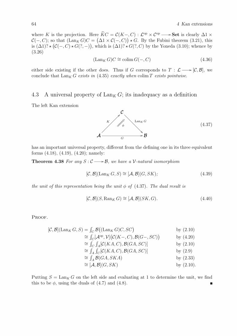
64 4 Kan extensions
where K is the projection. Here KC = C(K−, C) : Lop × Cop Set is clearly ∆1 ×C(−, C); so that (LanK G)C =
(∆1 × C(−, C)
) G. By the Fubini theorem (3.21), this
is (∆1)? (C(−, C) G(?,−)
), which is (∆1)? G(?, C) by the Yoneda (3.10); whence by
(3.26)
(LanK G)C ∼= colim G(−, C) (4.36)
either side existing if the other does. Thus if G corresponds to T : L [C,B], weconclude that LanK G exists in (4.35) exactly when colim T exists pointwise.
4.3 A universal property of LanK G; its inadequacy as a definition
The left Kan extension
A BG
C
A
K
C
B
LanK G
φ
(4.37)
has an important universal property, different from the defining one in its three equivalentforms (4.18), (4.19), (4.20); namely:
Theorem 4.38 For any S : C B, we have a V-natural isomorphism
[C,B](LanK G,S) ∼= [A,B](G,SK); (4.39)
the unit of this representation being the unit φ of (4.37). The dual result is
[C,B](S, RanK G) ∼= [A,B](SK,G). (4.40)
Proof.
[C,B](LanK G,S) =∫
CB
((LanK G)C, SC
)by (2.10)
∼=∫
C[Aop,V ]
(C(K−, C),B(G−, SC)
)by (4.20)
∼=∫
C
∫A[C(KA,C),B(GA,SC)] by (2.10)
∼=∫
A
∫C[C(KA,C),B(GA,SC)] by (2.9)
∼=∫
AB(GA,SKA) by (2.33)
∼= [A,B](G,SK) by (2.10).
Putting S = LanK G on the left side and evaluating at 1 to determine the unit, we findthis to be φ, using the duals of (4.7) and (4.8).

4.3 A universal property of LanK G; its inadequacy as a definition 65
Note that the left side of (4.39) exists in V (and not merely in some extension V ′) ifthe right side does; in particular
[C,B](LanK G,S) ∈ V if the domain A of K is small. (4.41)
Applying V = V0(I,−) : V0 Set to (4.39), we get a bijection of sets
[C,B]0(LanK G,S) ∼= [A,B]0(G,SK), (4.42)
which in view of (2.16) may be expressed as:
Theorem 4.43 If φ : G LK exhibits L as LanK G, then every V-natural α : G SKfactorizes as
A BG
C
A
K
C
B
S
A B
C
A
C
BL
φ
β (4.44)
for a unique β : L S.
The universal property of Theorem 4.43 can be satisfied by at most one (L, φ) to withinisomorphism; for it is a question of a representation [C,B]0(L, S) ∼= [A,B]0(G,SK). It ismoreover a very simple universal property, that makes sense not only in V-CAT but inany 2-category. This has led many authors to use it as the definition of left Kan extension.Let us call an (L, φ) with this universal property a weak left Kan extension of G alongK, writing L = lanK G with a small “l” (and ranK G for the dual). We now comparethis with our definition. Theorem 4.43 asserts that LanK G = lanK G if the former exists.However L = lanK G need not satisfy
[C,B](L, S) ∼= [A,B](G,SK), (4.45)
and hence by (4.39) need not be LanK G. Take V = Cat, with A a mere category andC = 1. The universal property of L = lanK G clearly asserts that L is the colimit of Gin B0, while (4.45) asserts that L is the colimit of G in B; yet by (3.54) the first of thesedoes not imply the second. (In this particular case, by (4.34), an L satisfying (4.45) isnecessarily LanK G.) Of course L = lanK G does satisfy (4.45) if V is conservative; it alsodoes so if B is cotensored, by an argument like that used in 3.8 when comparing conicallimits in B0 with those in B. Yet even an (L, φ) satisfying (4.45) still need not be LanK G;in other words, the isomorphism (4.39) is strictly weaker than our definition of LanK G.This is so even in the classical case V = Set; a counter-example is provided by (4.35),where LanK G exists by (4.36) precisely when T : L [C,B] has a pointwise colimit,while (4.45) merely asserts that L ∼= colim T , which by 3.3 does not imply pointwiseness.
For such reasons, various authors [22, 60, 9] who call lanK G a Kan extension use thename pointwise Kan extension for LanK G. Our present choice of nomenclature is based onour failure to find a single instance where a weak Kan extension plays any mathematicalrole whatsoever. (Street in [71] has given a definition of “pointwise Kan extension” in

66 4 Kan extensions
any 2-category with finite limits; it agrees with our notion when V = Set, but is strictlystronger for a general V , and is hence not suited to our context.)
When B is cotensored and L = lanK G exists, we have observed that L satisfies (4.45).If in this we now take for S the functor C(−, C) B for fixed C ∈ C and B ∈ B, we easilyget B(LC,B) ∼= [Aop,V ]
(C(K−, C),B(G−, B)
), so that L = LanK G by (4.20). Thus for
cotensored B there is no distinction between lanK G and LanK G. This is so in particularfor B = V ; moreover, since V is also tensored, ranK G and RanK G too have the samemeaning for B = V . This gives a way of defining RanK G, for any B, in terms of weakKan extensions:
Proposition 4.46 The diagram
A B ,G
C
A
K
C
B ,
T
ψ
exhibits T as RanK G if and only if, for each B ∈ B, the 2-cell B(B,ψ) exhibits B(B, T−)as ranK B(B,G−).
Proof. “Only if” is clear since representables preserve RanK G. For the converse,B(B, T−) is actually RanK B(B,G−) by the remark preceding the proposition; so that(4.8) is an isomorphism by (4.9) and (3.7), giving T = RanK G.
It is this way of defining RanK G, in terms of the universal property of ran, that isenvisaged in our remarks following Proposition 4.33.
Before leaving this comparison of Lan with lan, we should perhaps emphasize that,even when V is conservative, LanK G (or lanK G) has meaning heavily dependent on V .Thus, when V = Ab, LanK G is quite different from LanK0 G0. The former is an additivefunctor, and satisfies the universal property of Theorem 4.43 among all additive functors;the latter is in general not additive at all.
4.4 Iterated Kan extensions; Kan adjoints; [Aop,V ] as the free cocomple-tion of a small A
We continue with further elementary properties of Kan extensions which, in one way oranother, make use of Theorem 4.38 or Theorem 4.43.
Theorem 4.47 If LanK G exists we have
LanZ LanK G ∼= LanZK G, (4.48)
either side existing if the other does. Then if φ and θ are the units of LanK G andLanZ LanK G, the unit χ of LanZK G is the composite natural transformation in the dia-

4.4 Iterated Kan extensions; Kan adjoints; [Aop,V ] as the free cocompletion 67
gram
A B ,G
A
CK
C
DZ
D
B ,
M
C
B ,
L
φ
θ
where L denotes LanK G and M the common value in (4.48). If Z is fully faithful, LanK Gexists whenever LanZK G exists, being (LanZK G)Z.
Proof. (4.19) gives ZD LanK G ∼= (ZD.Kop) G, either side existing if the other does.
Since ZD.Kop = D(ZK−, D), this is by (4.18) the desired isomorphism (4.48). That theunits compose as shown is immediate from Theorem 4.43. The last statement comes fromthe easy observation that
ZKZ ∼= K if Z is fully faithful. (4.49)
If A and C are small, both [A,B] and [C,B] exist as V-categories; and any K : A Cinduces a V-functor [K, 1] : [C,B] [A,B] as in (2.26), sending S to SK. Then fromTheorem 4.38 we get the theorem of Kan adjoints:
Theorem 4.50 Let K : A C be a V-functor with A and C small. Then [K, 1] :[C,B] [A,B] has the left adjoint LanK if LanK G exists for all G : A B, as itsurely does when B is cocomplete; and [K, 1] has the right adjoint RanK if RanK G existsfor each G, as it surely does when B is complete.
We now consider the sense in which [Aop,V ], for a small A, is the free cocompletion ofA (embedded in [Aop,V ] by Yoneda).
Theorem 4.51 Let Y : A [Aop,V ] be the Yoneda embedding, where A is small, andlet B be arbitrary. Then for any cocontinuous S : [Aop,V ] B we have
S ∼= LanY G ∼= − G : [Aop,V ] B, (4.52)
whereG = SY : A B. (4.53)
Such a cocontinuous S has a right adjoint T given by
T = G : B [Aop,V ]. (4.54)
The full subcategory Cocts[[Aop,V ],B
]of
[[Aop,V ],B
]determined by the cocontinuous
functors exists as a V-category, and S → SY is an equivalence of V-categories
[Y, 1] : Cocts[[Aop,V ],B
] [A,B]′, (4.55)
68 4 Kan extensions
where [A,B]′ is the full subcategory of [A,B] determined by those G : A B for whichLanY G exists; the inverse to this equivalence sends G to LanY G. In particular, if B iscocomplete, this is an equivalence
Cocts[[Aop,V ],B
] [A,B]. (4.56)
Proof. Expressing an arbitrary F : Aop V as a small colimit F ∼= F Y ofrepresentables by (3.17), we see that a cocontinuous S must have SF ∼= F SY , whichis F G by (4.53), or (LanY G)F by (4.31). We then have B(SF,B) ∼= B(F G,B),∼=[Aop,V ](F, GB) by (3.5), so that S G.
Since the cocontinuous S is LanY G, it follows from (4.41) that Cocts[[Aop,V ],B
]exists as a V-category, and from (4.39) that
Cocts[[Aop,V ],B
](S, S ′) ∼=
[[Aop,V ],B
](LanY G,S ′) ∼= [A,B](G,S ′Y ) = [A,B](SY, S ′Y ).
Thus [Y, 1] in (4.55) is fully faithful. It is moreover essentially surjective, since if LanY G =− G exists, it is cocontinuous by (3.23), and (LanY G)Y ∼= G by Proposition 4.23 (orequally by (3.10)).
4.5 Initial diagrams as the left Kan extensions into V ; initial and finalfunctors when V = Set
As the motivation for our definition of right Kan extension, we chose in 4.1 the property(4.12) which allows us to write a limit FK,G as F, RanK G. We now examine thecorresponding problem of writing a limit H,TK in the form F, T.
First we need a result resembling (4.12) or (4.19), but where the Kan extension hascodomain V and the other functor need not:
Proposition 4.57 Let LanK H exist, where K : A C and H : A V; then for anyT : C B we have
LanK H,T ∼= H,TK , (4.58)
either side existing if the other does.
Proof. The formula (3.22) expressing the “continuity of a limit in its index” heregives H? C(K?,−), T− ∼= H?, C(K?,−), T−; but H? C(K−, ?) is LanK H by(4.18) and the symmetry (3.9), while C(K−, ?), T− ∼= TK by the Yoneda isomorphism(3.10).
Given now a diagram
A V ,H
C
A
K
C
V ,
F
φ
(4.59)

4.5 Initial diagrams as the left Kan extensions into V 69
we get for each T : C B a map
[C,V ](F,B(B, T−)) [A,V ](FK,B(B, TK−)) [A,V ](H,B(B, TK−)) , (4.60)
where the first arrow is [K, 1] and the second is [A,V ](φ, 1). This induces by (3.1) a map
(K,φ)# : F, T H,TK (4.61)
whenever these limits exist; it is the composite
F, TK∗
FK, TK φ,1 H,TK (4.62)
whenever the middle limit exists as well.
Theorem 4.63 For a diagram (4.59), the following are equivalent:
(i) For every B and every T : C B, the (K,φ)# of (4.61) is an isomorphism, eitherside existing if the other does.
(ii) For every B, every T : C B, and every B ∈ B, the map (4.60) is an isomorphism.
(iii) φ exhibits F in (4.59) as LanK H.
Proof. Clearly (ii) implies (i) by the definition of (3.1) of the limits, while (ii) itselfis, by (3.7), the special case of (i) obtained by replacing T in (4.61) by B(B, T−). Since(iii) implies (i) by Proposition 4.57, it remains only to prove that (i) implies (iii).
Let C ∈ C and Z ∈ V. Then applying (i) with B = V and with T = [C(−, C), Z] givesF, [C(−, C), Z] ∼= H, [C(K−, C), Z]. Since the internal-hom [X,Z] in V is the cotensorproduct X Z, the interchange-of-limits formula (3.20) lets us write the last isomorphismas C(−, C), [F−, Z] ∼= C(K−, C), [H−, Z]. By the Yoneda isomorphism (3.10), theleft side here is [FC,Z]; while by (3.7) the right side is [Aop,V ](C(K−, C),V(H−, Z)). Itnow follows from (4.20) that F , with unit φ, is LanK H.
When these equivalent conditions are satisfied, we say that the pair (K,φ) in (4.59)is initial . The characterization (i) of Theorem 4.63 is the assertion that the F -indexedlimit of any T is the H-indexed limit of TK, when either exists. The characterization(ii) is a V-enriched version of the assertion that, whether the limits exist or not, the(F,B)-cylinders over T coincide with the (H,B)-cylinders over TK. From the proof, it isimmaterial whether we require this only when the domain and codomain of (4.60) existin V , or when they exist merely in an extension V ′ as in 3.12.
For the dual notion we keep the diagram (4.59) as it is, but consider in place of T afunctor S : Cop B. Then (4.60) is replaced by a map
[C,V ](F,B(S−, B)) [A,V ](H,B(SK−, B)) , (4.64)
and (4.61) by a map(K,φ)# : H SKop F S . (4.65)
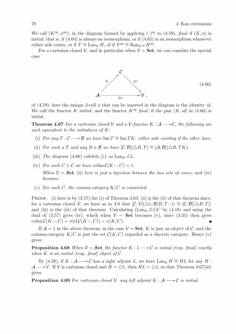
70 4 Kan extensions
We call (Kop, φop), in the diagram formed by applying ( )op to (4.59), final if (K,φ) isinitial; that is, if (4.64) is always an isomorphism, or if (4.65) is an isomorphism whenevereither side exists, or if F ∼= LanK H, of if F op ∼= RanKop Hop.
For a cartesian closed V , and in particular when V = Set, we can consider the specialcase
A V ,∆1
C
A
K
C
V ,
∆1
(4.66)
of (4.59); here the unique 2-cell φ that can be inserted in the diagram is the identity id.We call the functor K initial , and the functor Kop final , if the pair (K, id) in (4.66) isinitial.
Theorem 4.67 For a cartesian closed V and a V-functor K : A C, the following areeach equivalent to the initialness of K:
(i) For any T : C B we have lim T ∼= lim TK, either side existing if the other does.
(ii) For such a T and any B ∈ B we have [C,B]( B, T ) ∼= [A,B]( B, TK).
(iii) The diagram (4.66) exhibits 1 as LanK 1.
(iv) For each C ∈ C we have colim C(K−, C) = 1.
When V = Set, (ii) here is just a bijection between the two sets of cones; and (iv)becomes
(v) For each C, the comma-category K/C is connected.
Proof. (i) here is by (3.57) the (i) of Theorem 4.63; (ii) is the (ii) of that theorem since,for a cartesian closed V , we have as in 3.9 that [C,V ]( 1,B(B, T−)) ∼= [C,B]( B, T );and (iii) is the (iii) of that theorem. Calculating (LanK 1)C by (4.18) and using thedual of (3.57) gives (iv); which when V = Set becomes (v), since (3.35) then givescolim C(K−, C) = π(el C(K−, C)) = π(K/C).
If A = 1 in the above theorem, in the case V = Set, K is just an object of C; and thecomma-category K/C is just the set C(K,C) regarded as a discrete category. Hence (v)gives:
Proposition 4.68 When V = Set, the functor K : 1 C is initial [resp. final] exactlywhen K is an initial [resp. final] object of C.
By (4.28), if K : A C has a right adjoint L, we have LanK H ∼= HL for any H :A V . If V is cartesian closed and H = 1, then HL = 1; so that Theorem 4.67(iii)gives
Proposition 4.69 For cartesian closed V, any left adjoint K : A C is initial.

4.6 Filtered categories when V = Set 71
4.6 Filtered categories when V = Set; the commutativity in Set of fil-tered colimits with finite limits
Taking V = Set for this section, we recall for later use the notion of filtered category.There is an interplay between filtered and finite: an ordinary category P is finite if itsset of morphisms (and hence its set of objects) is finite. A category is finitely completeif it admits all (conical) limits indexed by finite categories; and a functor with a finitely-complete domain is left exact if it preserves all such finite limits: the duals are finitelycocomplete and right exact.
Theorem 4.70 For an ordinary category C, the following are equivalent:
(i) Every functor T : P C with P finite is the base of some inductive cone.
(ii) C is not empty; for any A,B ∈ C there is some C ∈ C and maps A C andB C; and for any maps f, g : A B in C there is some map h : B Dwith hf = hg.
(iii) For any finite category P the diagonal : C [P, C] has the property that T/ is non-empty for each T : P C.
(iv) For any finite category P the diagonal : C [P, C] is final.
Proof. The properties in (ii) are special cases of (i), and in turn imply (i) by a trivialinduction; while (iii) merely re-states (i). It remains to show that these imply (iv), whichby Theorem 4.67(v) is the requirement that the T/ in (iii) be not merely non-emptybut in fact connected. Given objects α and β of T/ – that is, cones (αP : TP A)and (βP : TP B) – we can find by (ii) maps f : A C and g : B C such thatfαP = gβP for each P ∈ P. This common value is now a cone (γP : TP C); and wehave maps f : α γ and g : β γ in T/ .
A category C satisfying these equivalent conditions is said to be filtered . It is clearthat a filtered category is connected, and also that [Q, C] is filtered if Q is finite and Cis filtered. Observe that a filtered-cocomplete category is filtered, since T : P C isthen the base of its colimit-cone; in this case, of course, : C [P, C] has a leftadjoint, which by Proposition 4.69 is stronger than being final. The initialness conditionof Theorem 4.67(v), or rather its dual, simplifies when C is filtered and K is fully faithful:
Proposition 4.71 If C is filtered, the fully-faithful K : A C is final if and only ifeach C/K is non-empty.
Proof. Only the “if” clause needs proof. Consider objects f : C KA andg : C KB of C/K. Because C is filtered, there are maps h : KA D andk : KB D with hf = kg; because D/K is non-empty we may suppose D to be of theform KE; because K is fully faithful, h and k have the form Ku and Kv. Thus f and gare connected in C/K by the maps u : f hf and v : g kg = hf .

72 4 Kan extensions
The classical example of this is that where C is a filtered preordered set (in which casedirected is often used for filtered), and K is the inclusion of a subset A. To say that eachC/K is non-empty is then to say that each C ∈ C is less than or equal to some A ∈ A.Such a subset A, which we call final, was classically called cofinal.
A filtered colimit is a conical one indexed by a small filtered category. For example,suppose we have in any category a coproduct A =
∑x∈X Ax. The finite subsets J of
X, ordered by inclusion, form a filtered ordered set C; and if the finite coproduct AJ =∑x∈J Ax exists for each J ∈ C, it is clear that A is the filtered colimit of the AJ .Recall from (3.35) that colim F for F : C Set is π(el F ).
Theorem 4.72 For F : C Set where C is small and filtered, two objects (A, x) and(B, y) of el F have the same image in π(el F ) = colim F if and only if there are mapsf : A C and g : B C with (Ff)x = (Fg)y.
Proof. The relation between (A, x) and (B, y) expressed by the existence of such fand g is reflexive and symmetric, and clearly generates the equivalence relation of beingconnected. It therefore coincides with this latter if it is transitive; and that it is so followseasily from the filteredness.
If B is an equational category of algebras whose operations all have finite arity, theconservative forgetful functor U : B Set preserves (and therefore reflects) filteredcolimits. For if F : C B with C small and filtered, any finite number of elements ofX = colim UF can by the filteredness be represented by elements (C, xi) ∈ el(UF ) with acommon C, so that we can apply an n-ary operation ω to get ω(x1, . . . , xn) ∈ UFC. ByTheorem 4.72, the image of this in X is independent of the choice of C; thus X becomesUA for an algebra A, which is clearly the colimit of F .
Theorem 4.73 Filtered colimits commute with finite limits in Set. That is to say, ifF : P × C Set with P finite and C small and filtered, the evident canonical map
ρ : colimC limP F (P,C) limP colimC F (P,C)
is an isomorphism.
Proof. By (3.28) and (3.35), an element of limP colimC F (P,C) is a cone (αP :1 π(el F (P,−))). By the filteredness of C we can find representatives (C, xP ∈F (P,C)) of the αP , with a common C. For f : P Q in P, the objects (C,F (f, C)xP )and (C, xQ) represent the same element of π(el F (Q,−)), because α is a cone. Since thereare but a finite number of maps in P, we can by the filteredness of C find a g : C Din C such that (D,F (f, g)xP ) = (D,F (Q, g)xQ) for each map f : P Q in P. Nowthe yP = F (P, g)xP constitute a cone with vertex 1 over F (−, D), or an element y oflimP F (P,D). If z is the image of this in colimC limP F (P,C), we clearly have ρ(z) = α;thus ρ is surjective.
To see that ρ is injective, suppose that y ∈ limP F (P,D) and y′ ∈ limP F (P,D′)represent elements of colimC limP F (P,C) with the same image under ρ. Then yP ∈F (P,D) and y′
P ∈ F (P,D′) represent for each P the same element of colimC F (P,C). Asin Theorem 4.72, but using the filteredness to do it simultaneously for each P ∈ P, wecan find h : D E and h′ : D′ E such that F (P, h)yP = F (P, h′)y′
P = wP say.
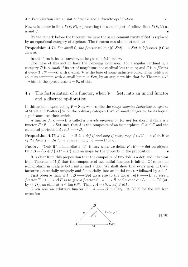
4.7 Factorization into an initial functor and a discrete op-fibration 73
Now w is a cone in limP F (P,E), representing the same object of colimC limP F (P,C) asy and y′.
By the remark before the theorem, we have the same commutativity if Set is replacedby an equational category of algebras. The theorem can also be stated as:
Proposition 4.74 For small C, the functor colim : [C,Set] Set is left exact if C isfiltered.
In this form it has a converse, to be given in 5.10 below.The ideas of this section have the following extension. For a regular cardinal α, a
category P is α-small if its set of morphisms has cardinal less than α; and C is α-filteredif every T : P C with α-small P is the base of some inductive cone. Then α-filteredcolimits commute with α-small limits in Set, by an argument like that for Theorem 4.73– which is the special case α = ℵ0 of this.
4.7 The factorization of a functor, when V = Set, into an initial functorand a discrete op-fibration
In this section, again taking V = Set, we describe the comprehensive factorization systemof Street and Walters [74] on the ordinary category Cat0 of small categories; for its logicalsignificance, see their article.
A functor J : C B is called a discrete op-fibration (or dof for short) if there is afunctor F : B Set such that J is the composite of an isomorphism C ∼= el F and thecanonical projection d : el F B.
Proposition 4.75 J : C B is a dof if and only if every map f : JC B in B isof the form f = Jg for a unique map g : C D in C.
Proof. “Only if” is immediate; “if” is easy when we define F : B Set on objectsby FB = D ∈ C | JD = B and on maps by the property in the proposition.
It is clear from this proposition that the composite of two dofs is a dof; and it is clearfrom Theorem 4.67(i) that the composite of two initial functors is initial. Of course anisomorphism in Cat0 is both initial and a dof. We shall show that every map in Cat0
factorizes, essentially uniquely and functorially, into an initial functor followed by a dof.First observe that, if F : B Set gives rise to the dof d : el F B, to give a
functor T : A el F is to give a functor S : A B and a cone α : 1 FS (or,by (3.28), an element α ∈ lim FS). Then TA = (SA, αA) ∈ el F .
Given now an arbitrary functor S : A B in Cat0, let (F, φ) be the left Kanextension
A Set .∆1
B
A
S
B
Set .
F=LanS ∆1
φ
(4.76)

74 4 Kan extensions
By (4.18), (3.26), and (3.35) we have
FB = B(S−, B) 1 ∼= colimB(S−, B) ∼= π(S/B) . (4.77)
The functor S, together with the cone φ : 1 FS, constitutes a functor T : A el Fwith dT = S. We shall have factorized S in the desired way if we show that T is initial.
This seems to be best done by a direct calculation using Theorem 4.67(v). (Thepurported proof in [74] is erroneous; it supposes that, in the situation of our Theorem 4.47,if X and θ are left Kan extensions, so is φ; that this is false is easily seen by taking D = 1and using (4.34).)
A typical object of el F , by (4.77), is (B, [f ]) where [f ] is the connected componentof some f : SA B. It is clear that T : A el F sends A to (SA, [1SA]) and sendsh : A A′ to Sh. An object of the comma-category T/(B, [f ]) is at once seen to be apair (A, g : SA B) with [g] = [f ]. A morphism (A, g) (A′, g′) is an h : A A′
for which g′Sh = g. It follows that T/(B, [f ]) is connected, being isomorphic to theconnected component [f ] of S/B.
To see that this factorization is essentially unique and functorial – that is, that wehave a factorization system in the sense of [30] – it remains to show the existence of aunique “diagonal” R : D A in any commutative diagram
A B ,d
C
A
P
C DK D
B ,
Q
where K is initial and d is a dof. We may as well suppose at once that A = el F for someF : B Set. Then P corresponds as above to a functor S : C B with dP = S, and acone α : 1 FS = FdP = FQK. Since K is initial, this cone is by Theorem 4.67(ii)of the form α = βK for a unique cone β : 1 FQ. Now Q and β constitute a functorR : D A with dR = Q, and clearly with RK = P . It is evident that any R′ : D Awith dR′ = Q and R′K = P must coincide with R. This completes the proof.
If we write dof/B for the full subcategory of Cat0/B determined by those J : A Bthat are dofs, it is clear that this factorization gives a reflection Cat0/B dof/B. Onthe other hand dof/B is evidently equivalent to [B,Set]. Thus we get an adjunction
Ω Θ : [B,Set] Cat0/B , (4.78)
with Θ fully faithful. Here Θ sends F : B Set to d : el F B, and may be calledthe discrete Grothendieck construction; its left adjoint Ω sends S to the F of (4.77).
While this is special to the case V = Set, it has generalizations to the importantcases V = Gpd and V = Cat, the latter being the setting for the original Grothendieckconstruction [34]. We do not give these here, for they transcend the context of enriched

4.8 The general representability and adjoint-functor theorems 75
category theory as developed in this account, and involve “transformations” more generalthen the Gpd-natural or Cat-natural ones; we shall treat them in [46].
Note finally that ΩΘS ∼= S, since Θ is fully faithful. This means by (4.76) that, forany F : B Set, we have a left Kan extension
el F Set ;∆1
B
el F
d
B
Set ;
F
φ
(4.79)
since this asserts by (4.77) that FB ∼= colimB(d−, B), it is precisely a restatement of(3.32).
4.8 The general representability and adjoint-functor theorems; the specialcase of a complete domain-category
In this section and the next we look at conditions ensuring the representability of a V-functor F : C V , especially in the simplest case of a complete C. Since by 1.11 theV-functor T : C B has a left adjoint precisely when each B(B, T−) is representable,the same considerations yield conditions for a left adjoint to exist.
Since a colimit in C is itself the representing object for a functor C V , the rep-resenting object for F : C V , if it exists, is in some sense a “generalized colimit”.Representing objects are, in fact, very commonly constructed as colimits: consider someexamples. First, in the case V = Set, a representation for F corresponds, as we observedin 1.10, to an initial object in el F ; that is, to the colimit of the empty diagram in el F .Next, in Proposition 3.36, a functor F : C V was in effect given as an iterated limit ofrepresentables; and we constructed its representing object as the corresponding iteratedcolimit of the representing objects for these. Again, the left Kan adjoint LanK of Theorem4.50 was constructed via the colimits KC ∗ G. A free abelian group is constructed as acoproduct of infinite cyclic groups; the tensor product of two abelian groups is constructedas a cokernel of a free abelian group; and the free monoid on a set X is the coproduct∑
n≥0 Xn. More generally, numerous constructions of free algebras, free monoids, and freemonads, as iterated colimits, under cocompleteness but no completeness hypotheses, aregiven in [44].
Yet the only general necessary condition that we so far have for the representabilityof F is expressed in terms of limits: by 3.2, F must preserve whatever limits exist.Hence if C is complete, F must be continuous (and similarly for a T : C B thatis to have a left adjoint). We here consider what must be added to this continuity toensure representability (or existence of an adjoint). Since the desired representing objectis a generalized colimit, this is analogous to the question of what must be added to
76 4 Kan extensions
completeness to ensure cocompleteness – or rather, to ensure the existence of a particularcolimit.
A small complete Set-category C is of necessity a preordered set – for if C(A,B) hadat least two elements, C(A,Bn) would have at least 2n, making C large if Bn existedfor all small cardinals n. Hence, by the classical argument on complete lattices, a smallcomplete C is also cocomplete: the supremum of a subset is the infimum of its set ofupper bounds. Not so, if C is large – even if C is a preordered set: the ordered set of smallordinals is cocomplete but not complete. What must be added is a condition ensuringthat the colimit we need can be manufactured from small limits. Similarly in the case ofrepresentability of F : C V : the extra condition needed is a “smallness” one on F .
We begin with a general result expressing a representing object as a limit: a large one,unless C happens to be small.
Theorem 4.80 F : C V is representable if and only if the limit F, 1C ex-ists and is preserved by F . Then the representing object is F, 1, and the counitµ : F C(F, 1,−) of this limit is an isomorphism giving the representation of F .
Proof. One direction is immediate: if F is the representable C(D,−), then by (3.10)the limit C(D,−), 1 is D, with counit µ = 1 : C(D,−) C(D,−); similarly, withappropriate changes, when F is only isomorphic to C(D,−); and the representable Fpreserves this limit.
For the other direction we have by hypothesis that
F µ C(F, 1,−)
F [FF, 1, F−]
is the counit of the limit F, F. Hence by (3.4) the (F, I)-cylinder over F given by theisomorphism i : F [I, F−] has the form i = [g, 1]Fµ for a unique g : I FF, 1.Writing λ : C(F, 1,−) F for the composite i−1[g, 1]F , we therefore have λµ = 1;and to prove µ an isomorphism it remains to show that µλ : C(F, 1,−) C(F, 1,−)is 1.
But by Yoneda, this map µλ is C(f, 1) for a unique f : F, 1 F, 1. Since λµ = 1we have µλµ = µ, or C(f, 1)µ = µ = C(1, 1)µ. However, as the counit of the limit F, 1,the cylinder µ factorizes through itself as C(f, 1)µ for a unique f ; whence f = 1 andµλ = 1.
There is a corresponding adjunction theorem:
Theorem 4.81 T : C B has a left adjoint if and only if RanT 1C exists and is preservedby T . Then the left adjoint S is RanT 1, and the counit ST 1 of the Kan extensionis the counit of the adjunction.
Proof. If S T we have RanT 1 ∼= S by (the dual of) (4.28); that the counit is asdescribed is immediate; and the right adjoint T preserves the right Kan extension.
For the converse, observe that (RanT 1)B = B(B, T−), 1 by (4.9). This limit is,by hypothesis, preserved by T : hence it is also preserved by B(B, T−). Thus B(B, T−)is representable by Theorem 4.80. This being for all B, we conclude that T has a leftadjoint.

4.9 Representability and adjoint-functor theorems when V = Set 77
Combining Theorem 4.63 with Theorem 4.80 gives the following, which replaces thelarge limit F, 1 by one that may be smaller:
Proposition 4.82 Let F : C V be LanK H, where K : A C and H : A V.Then F is representable if and only if the limit H,K exists and is preserved by F ; andthe representing object is then H,K.
We consider the possibility of a small A here:
Proposition 4.83 The following properties of F : C V are equivalent:
(i) F is a small (indexed) colimit of representables.
(ii) F has the form LanK H where the domain A of K is small.
(iii) F is the left Kan extension of its restriction to a small full subcategory of C.
Proof. To say that F is a small colimit of representables is to say that we have a smallindexing-type H : A V and a functor K : A C such that, if Y : Cop [C,V ]is the Yoneda embedding ([C,V ] being a V ′-category for some suitable extension V ′ ofV), we have H ∗ Y Kop ∼= F . Since small colimits in [C,V ] exist pointwise by 3.3, this isto say that H ∗ C(K−, C) ∼= FC for each C; and hence by (4.18) and (3.9) to say thatF = LanK H. Thus (i) and (ii) are equivalent. It remains to show that, if we have (ii),we also have its special case (iii).
For this, let A′ be the full image of K : A C, so that K factorizes as say W :A A′ followed by the inclusion Z : A′ C. Then A′ is still small; and because Zis fully faithful, we have F ∼= LanZ FZ by Theorem 4.47.
We shall call a functor F : C V satisfying the equivalent properties of Proposition4.83 accessible. In particular every representable C(D,−) : C V is accessible; it isin fact LanD I where D : I C and I : I V . So Proposition 4.82 now gives ourdesired representability theorem for complete C:
Theorem 4.84 If C is complete, F : C V is representable if and only if it is continuousand accessible.
For a general complete C, the representability of F is not implied by its continuityalone, even in the case V = Set. The classical counter-example takes for C the categoryof (small) groups, and for F : C Set the functor given by FC =
∏α C(Gα, C), where
Gα is the large set of all small simple groups.
4.9 Representability and adjoint-functor theorems when V = Set
Although Theorem 4.84 gives a simple general criterion that we shall use below in 5.6,it is often advantageous, in considering the representability of a particular V-functor, toreduce the problem to the more familiar case V = Set by using:

78 4 Kan extensions
Theorem 4.85 Let C admit cotensor products. Then the V-functor F : C V isrepresentable if and only if the ordinary functor
C0 F0
V0 V Set
is representable and F preserves cotensor products. Moreover a V-functor T : C B hasa left adjoint if and only if the ordinary functor T0 : C0
B0 does so and T preservescotensor products.
Proof. “Only if” is clear both in the representability case and in the adjunction case– in the former, if F ∼= C(D,−), then V F0
∼= C0(D,−) by (1.33).For the converse, let β : C0(D,−) ∼= V F0 be a representation with unit η ∈ V FD; then
η : I FD corresponds by Yoneda to a map α : C(D,−) F , which we show to bean isomorphism. It suffices to verify that V0(X,αC) : V0(X, C(D,C)) V0(X,FC) isan isomorphism for each C ∈ C and each X ∈ V. The domain here is isomorphic by (3.45)to C0(D,X C), and the codomain by (1.25) to V [X,FC], which is then isomorphic toV F (X C) since F preserves cotensor products. It is easily verified that, modulo theseisomorphisms, V0(X,αC) is in fact the isomorphism βXC .
The case of adjoints follows from this, since B0(B, T−) = V (B(B, T−))0 by (1.33) andsince, if T preserves cotensor products, so does B(B, T−).
We accordingly take V = Set for the rest of this section. Recall that, in taking C tobe a Set-category, we are automatically supposing it to be locally small. There are manyclassical results on the representability of F : C Set; and to reproduce them herein detail, with examples of their use, would involve an unjustifiably long digression fromour main path of development. Some briefer comments may however be useful. First,whether C is complete or not, applying Proposition 4.82 to the left Kan extension (4.79)gives:
Proposition 4.86 F : C Set is representable if and only if d : el F C has a limitwhich is preserved by F ; the representing object is then lim d.
The following proposition is useful in various contexts; it follows at once from theobservation in 4.6 that a functor T : A el F consists of a functor S = dT : A Cand an α ∈ lim FS:
Proposition 4.87 If C admits the conical limits of some class, and F : C Setpreserves them, then el F also admits such limits, and d : el F C preserves andreflects them. In particular, el F is complete if C is complete and F is continuous.
By 3.4 and Proposition 4.83, F : C Set is accessible precisely when it is a smallconical colimit of representables. There is a weaker condition – strictly weaker by [29] –related to this as finite-generation of an algebra is related to finite-presentability: namelythat F be an epimorphic image of a small coproduct of representables; call this weakaccessibility. Consider what it means. A map C(Dα,−) F corresponds by Yonedato an object (Dα, yα ∈ FD) of el F . Since epimorphisms in [C,Set] are pointwise, to saythat
∑α C(Dα,−) F is epimorphic is to say that every (C, x) ∈ el F admits a map

4.9 Representability and adjoint-functor theorems when V = Set 79
from some (Dα, yα). If S is the small full subcategory of el F determined by the objects(Dα, yα), and J : S el F is the inclusion, this is to say that the comma-categoryJ/(C, x) is non-empty for each (C, x).
When el F is complete, however – or even finitely complete – so that (el F )op is filtered,the non-emptiness of each J/(C, x) implies by Proposition 4.71 the initialness of J :S el F . Thus from Theorem 4.84, Proposition 4.86, Proposition 4.87, and Theorem4.67, we get Freyd’s General adjoint functor theorem (cf. [28]):
Theorem 4.88 For F : C Set where C is locally-small and complete, the followingare equivalent:
(i) F is representable.
(ii) F is continuous and accessible.
(iii) F is continuous and weakly accessible.
Then the representing object for F is lim dJ .
The weak accessibility of F is often called the solution-set condition. Since C is locallysmall, it can be expressed as follows: there is a small set T of objects of C such that, forany C ∈ C and any x ∈ FC, there is some E ∈ T some y ∈ FE and some f : E Cwith (Ff)y = x.
Recall that we also have the quite elementary observation from 1.10:
Proposition 4.89 For F : C Set the following are equivalent:
(i) F admits a representation α : C(D,−) ∼= F with unit η ∈ FD.
(ii) el F has an initial object (D, η).
(iii) ∆1 : el F Set is representable by (D, η).
Applied to ∆1 : E Set for any Set-category E , Theorem 4.88 gives that E hasan initial object if it is complete and has a small full subcategory S (the “solution set”)such that any E ∈ E admits a map from some S ∈ S. Conversely we could have provedTheorem 4.88 alternatively by using Proposition 4.89 and Proposition 4.87 to reduceit to this “initial-object theorem”, and by giving a simple direct proof of the latter.In discussing variants of Theorem 4.88, we take this approach for brevity: we describethe corresponding initial-functor theorem, and leave the reader to translate it back to arepresentability theorem.
An unpublished result of Freyd, given in lectures in 1970, deals with a non-completeE . It asserts that E has an initial object if and only if (i) E satisfies the solution-setcondition as above, (ii) every A ∈ E has a map from some B ∈ E all of whose idempotentendomorphisms split, and (iii) every small diagram in E admits some projective coneover it. The corresponding representability theorem, with C the (non-complete) stablehomotopy category of CW-complexes, gives Brown’s result [11] on the representability ofcohomology theories.

80 4 Kan extensions
Very commonly, E is not only complete but admits arbitrary (even large) intersectionsof subobjects; by Proposition 4.87, elF is so if C is so and if F preserves, besides smalllimits, all intersections of subobjects. For such an E , the intersection of all the subobjectsof E ∈ E is an atom – an object with no proper subobject. So the set S of isomorphism-classes of atoms in E forms a solution-set if it is small. In many concrete cases, it iseasy to find a small cardinal exceeding cardS; this is probably the most common way ofapplying Theorem 4.88.
The adjoint-functor theorem of Day [15], in its initial-object-theorem form, requiresonly partial completeness of E : the existence of equalizers, of pullbacks of monomorphisms,and of arbitrary intersections of subobjects; but it strengthens the solution-set conditionto the requirement that there is some S ∈ E such that, for each A ∈ E , there is amonomorphism A B and a map S B. Then the atom in S is the initial object.Since this refers to no infinite limits except intersections of monomorphisms, it has ananalogue [18] in an elementary topos, where such intersections exist in an internal sense.
Day’s result also yields a proof of Freyd’s Special Adjoint Functor Theorem (cf. [28]):
Theorem 4.90 If the locally-small C is complete, admits all intersections of subobjects,and has a small cogenerating set, every continuous F : C Set is representable.
Proof. It is clear that E = el F has a small cogenerating set Gα in these conditions.The hypothesis of Day’s initial-object theorem are clearly satisfied with S =
∏α Gα and
with A B the canonical monomorphism A ∏
α(E(Gα, A) Gα).
Applying this to the existence of a left adjoint to the diagonal ∆ : C [A, C], we seethat C is cocomplete if it is complete, admits intersections of subobjects, and has a smallcogenerating set.
4.10 Existence and characterization of the left Kan extension along afully-faithful K : A C in terms of cylinders in C sent to colimitsby the C(KA,−)
For cocomplete B, the left Kan extension of G : A B along K : A C exists by(4.13) if A is small. By Theorem 4.47, it still exists when A is not small, provided that Kis itself a left Kan extension along some A′ A with A′ small. We now turn to existenceresults when B is no longer cocomplete, but admits colimits only of some specified class.
Theorem 4.91 The left Kan extension of G : A B along K : A C exists if andonly if, for each C ∈ C, the functor KC : Aop V can be so expressed as a colimitF ∗ Y Q of representables that the colimit F ∗ GQ exists in B; then this latter colimit is(LanK G)C.
Proof. Let KC be so expressible, where F : Lop V and Q : L A. Since(Y Q−) ∗ G ∼= GQ by (3.10), we have from (3.23) that KC ∗ G = (F ∗ Y Q) ∗ G exists,being F ∗ ((Y Q−)∗G) ∼= F ∗GQ. For the converse, we just take the canonical expression
(3.17) of KC as a colimit of representables, corresponding to F = KC and Q = 1.

4.10 Existence and characterization of the left Kan extension 81
As an example of this, take V = Set, let Gxx∈X be a small set of objects in thecocomplete category C, and let A be the full subcategory of C determined by the smallcoproducts of the Gx, with K : A C the inclusion. For any C ∈ C, let ε : D =∑
x∈X C(Gx, C)·GxC be the canonical map whose (x, f)-component, for f ∈ C(Gx, C),
is f . Write Mx for the set of pairs of maps g, h : Gx D such that εg = εh, and let
φ, ψ : E =∑
x Mx · Gx D be the maps whose respective (x, g, h)-components are g
and h. The commutative diagram
Eφ
ψ D ε
C (4.92)
is not in general a coequalizer diagram; but for each x the diagram
C(GX , E)C(1,φ)
C(1,ψ) C(GX , D) C(1,ε)
C(GX , C) (4.93)
is a split coequalizer diagram. That is to say, there are maps t : C(Gx, C) C(Gx, D) ands : C(Gx, D) C(Gx, E) for which C(1, ε)t = 1, C(1, φ)s = 1, and C(1, ψ)s = tC(1, ε);which easily implies that (4.93) is a coequalizer. To wit, t(f) : Gx
D is the coprojectionix,f of the coproduct, while s(u) : Gx
E is the coprojection corresponding to the index(x, u, ix,εu). Any product of the diagrams (4.93) over a family (xj) of the indices x is clearly
again a split coequalizer; whence it follows that K sends (4.92) to a coequalizer diagram
A(−, E) A(−, D) KC
in [Aop,Set]. We conclude that the left Kan extension of G : A B along K : A Cexists whenever B admits coequalizers, and is given as the coequalizer of the two mapsGφ,Gψ : GE GD. (We remark that, when (4.92) is a coequalizer diagram for eachC, Gx is said to be a regular generator of C; it is easily verified to be a fortiori astrong generator and a generator.) Clearly Theorem 4.91 could be so modified as to cover
the case where KC was expressed as an iterated colimit of representables. There is aparticularly neat and useful result of this kind when K is fully faithful; which we nowsuppose.
Let F : Lop V , let P : L C be a diagram of type F , let C ∈ C, and letα : F C(P−, C) be an (F,C)-cylinder over P , in the language of 3.1. Let us say thatα is a K-cylinder if the composite cylinder
F α C(P−, C)
K
[Aop,V ](KP−, KC)
is a colimit-cylinder, givingKC ∼= F KP. (4.94)
For this it certainly suffices that, for each A ∈ A, the cylinder
F α C(P−, C) C(KA,−)
[C(KA,P−), C(KA,C)]
82 4 Kan extensions
be a colimit-cylinder, so that
C(KA,C) ∼= F C(KA,P−) ; (4.95)
this is just the pointwise existence of the colimit (4.94); and by 3.3 the pointwiseness isautomatic if L is small.
An expression of KC as a colimit F ∗ Y Q of representables, as in Theorem 4.91, hasas unit a cylinder β : F [Aop,V ](Y Q−, KC). The codomain of β is isomorphic by
Yoneda to (KC)Qop = C(KQ−, C); moreover, since K is fully faithful, we have Y ∼= KKby (4.22). It follows that β has the form
F α C(KQ−, C)
K
[Aop,V ](KKQ−, KC) , (4.96)
in which the second map is in fact an isomorphism. Thus such an expression of KC as acolimit of representables is the same thing as a K-cylinder in which P factorizes throughA as KQ.
In this fully-faithful case we have a characterization of LanK G as follows:
Theorem 4.97 An extension S : C B of G : A B along the fully-faithfulK : A C is LanK G (that is, S is canonically isomorphic to LanK SK) if and only ifit sends each K-cylinder to a colimit-cylinder. If A is small, it suffices to speak of smallK-cylinders.
Proof. The canonical expression of KC as a colimit KC ∗ Y of representables cor-responds as in (4.96) to a K-cylinder 1 : KC C(K−, C). If S sends this to a
colimit-cylinder we have SC ∼= KC ∗ SK, which is KC ∗ G since S is an extension of G;thus S ∼= LanK G. Conversely, if LanK G exists, any K-cylinder α is, by definition, sentto a colimit-cylinder by K; by (3.23) the functor −∗G preserves the colimit (4.94), since
each KPL ∗ G exists; hence LanK G = K− ∗ G sends α to a colimit-cylinder.
Still supposing K fully faithful, consider a family Φ = (αγ : Fγ C(Pγ−, Cγ))γ∈Γ
of K-cylinders, where Fγ : Lopγ
V and Pγ : Lγ C. Generalizing 3.5, where it was
a question of a family of colimits, we say that C is the closure of A under the family Φif there is no proper replete full subcategory D of C, containing A, and such that Cγ ∈ Dwhenever Pγ takes its values in D.
Theorem 4.98 Let K : A C be fully faithful, and let C be the closure of A for a familyΦ of K-cylinders as above. Then a functor S : C B is exhibited by 1 : SK SKas LanK SK if and only if S sends each cylinder of Φ to a colimit-cylinder. MoreoverLanK G exists for any G : A B if B admits Fγ-indexed colimits for each γ ∈ Γ.
Proof. Theorem 4.97 gives the necessity in the first assertion. For the suffi-ciency, let D be the replete full subcategory of C consisting of those C for whichS : C(K−, C) B(SK−, SC) as unit exhibits SC as KC ∗ SK. Then A ⊂ D since
we have canonical isomorphisms SKA ∼= Y A ∗ SK ∼= KKA ∗ SK. If Pγ takes its
values in D, we have a canonical isomorphism KPγ− ∗ SK ∼= SPγ by the definition of
D; and KCγ∼= Fγ ∗ KPγ by (4.94). Hence (3.23) gives Fγ ∗ SPγ
∼= KCγ ∗ SK. Since

4.10 Existence and characterization of the left Kan extension 83
Fγ ∗ SPγ∼= SCγ by hypothesis, we have Cγ ∈ D; thus D is all of C, as desired. The
second assertion is proved by a similar argument, taking D to consist of those C for whichKC ∗ G exists.
For an example of this, let us modify the example following Theorem 4.91. Withthe notation as there, write A′ for the full subcategory of C determined by the finitecoproducts of the Gx. Since every coproduct is the filtered colimit of the finite coproductsof its summands, every object of A is a filtered colimit of objects of A′. Suppose now thateach Gx is finitely presentable – meaning that each C(Gx,−) : C Set preserves filteredcolimits. Then, since filtered colimits commute with finite limits in Set by Theorem 4.73,each object of A′ is finitely presentable; and thus the filtered colimits in question arepreserved by Z : C [A′op,Set], where Z is the inclusion A′ A C; that is,they correspond to Z-cylinders. It now follows from Theorem 4.98 that any G : A′ Badmits a left Kan extension along Z : A′ C if B admits coequalizers and filteredcolimits.
We end with a result, a special case of which we have already used in Theorem 4.51:
Theorem 4.99 Let K : A C be fully faithful, and denote by [A,B]′ the full subcategoryof [A,B] determined by those G for which LanK G exists. Then LanK : [A,B]′ [C,B]is fully faithful; so that we have an equivalence [A,B]′ [C,B] , where the latter is the fullsubcategory of [C,B] determined by the functors isomorphic to some LanK G; the inverseto this equivalence is composition with K. If A is small, it follows that [C,B] is a Vcategory.
Proof. We have by Theorem 4.38 that [C,B](LanK G, LanK G′) ∼= [A,B](G, (LanK G′)K),which by Proposition 4.23 is isomorphic to [A,B](G,G′).
Of course this fully-faithfulness is just a special case of the observation in 1.11 following(1.53), to which we could have appealed: for we are dealing with an adjunction LanK [K, 1] whose unit φ is an isomorphism. In practice we use the equivalence [A,B]′ [C,B]
chiefly when [A,B]′ is all of [A,B], as for instance under the hypotheses of Theorem 4.98or when A is small and B is cocomplete.
84 4 Kan extensions

Chapter 5
Density
5.1 Definition of density, and equivalent formulations
A function k : A C, not necessarily continuous, between hausdorff spaces is dense(in the sense that its image is a dense subset) precisely when any continuous map from Cinto another hausdorff space B is uniquely determined by its composite with k; that is,when Set(k, 1) : Haus(C,B) Set(A,B) is injective. We give an analogous definitionof density for a V-functor K : A C.
For a V−category C, the functor category [C,B] exists at least as a V ′-category forsome suitable extension V ′ of V as in 3.12. Consider those S : C B which preserveevery colimit existing in C whose indexing-type F : Aop V has domain Aop; these con-stitute a full subcategory A- Cocts[C,B], which if A is small contains the full subcategoryCocts[C,B]of those S preserving all small colimits that exist.
Theorem 5.1 For A V-functor K : A C the following are equivalent:
(i) For any B, the restriction to A- Cocts[C,B] of the functor [K, 1] : [C,B] [A,B]is fully faithful.
(ii) The functor K : C → [Aop,V ] is fully faithful.
(iii) For each C,D ∈ C the map K : C(C,D) [Aop,V ](C(K−, C), C(K−, D)) is anisomorphism.
(iv) For each C ∈ C, the identity cylinder 1: C(K−, C) C(K−), C) as unit exhibits
C as KC K.
(v) The identity 1 : K 1CK exhibits 1C as LanK K.
(vi) Some isomorphism φ : K 1CK exhibits 1C as LanK K.
Proof. Because a representable Cop V preserves all limits that exist, its dualC Vop preserves all colimits that exist in C. Since the Yoneda embedding is fullyfaithful, and since K is the composite
CY
[Cop,V ][Kop,1]
[Aop,V ],
85
86 5 Density
it follows that (i) implies (ii). The direct translation (iii) of (ii) is equivalent by (3.5) to(iv), which is in turn equivalent by (4.18) to (v), itself a special case of (vi); so that it re-mains only to show that (vi) implies (i). Suppose then that S : C B is A-cocontinuous;
it thus preserves the colimit KC K, and hence the left Kan extension in (vi), so thatSφ : SK SK exhibits S as LanK(SK). By Theorem 4.38 we therefore have for anyS ′ : C B a representation [C,B](S, S ′) ∼= [A,B](SK, S ′K), whose unit is Sφ. By(1.48), this isomorphism is the composite of [K, 1] : [C,B](S, S ′) [A,B](SK, S ′K)and [A,B](Sφ, 1) : [A,B](SK, S ′K) [A,B](SK, S ′K); the latter being an isomorphismsince φ is, so is the former – which proves (i).
A V-functor K : A C satisfying these equivalent conditions is said to be dense.(The original term used by Isbell, who introduced the concept for V = Set in [35], wasleft adequate.) For the dual notion (Isbell’s right adequate) we use codense; K : A Cis codense if Kop : Aop Cop is dense. In the important special case where the denseK : A C is the inclusion of a full subcategory, we merely say that A is dense in C,leaving K to be understood; and if A is the one-object full subcategory A, we say thatA is dense in C.
It is clear that the density of K depends only on “the equivalence class of K in the2-category of V-functors”; that is, if K is dense, so is the composite
A A −→K′
C C (5.2)
where the outer functors are equivalences and where K ′ is isomorphic to K.When C admits tensor products, the criterion (v) for the density of K : A C
becomes by (4.25) the requirement that the canonical map C(KA,C)⊗KA C expressC as the coend
C ∼=∫ A
C(KA,C) ⊗ KA ; (5.3)
while when V = Set it becomes by (4.27) the requirement that the canonical cone expressC as the colimit
C ∼= colim(K/C −→d
A −→K
C) . (5.4)
If K : A C is dense, applying V : V0 Set to the isomorphism in Theorem
5.1(iii) above gives a bijection of sets
C0(C,D) ∼= [Aop,V ]0(C(K−, C), C(K−, D)) , (5.5)
whose meaning is that every V-natural transformation α : C(K−, C) C(K−, D) is ofthe form C(K−, f) for a unique f : C D. It is clear that (5.5) is in turn equivalent tothe density of K if V is conservative, and in particular in the classical case V = Set. It isalso equivalent to density if C is cotensored; or even if C admits cotensor products Xβ Cfor some set Xβ constituting a strong generator of V0: for if we write (5.5) with X Din place of D, we easily get V0(X, C(C,D)) ∼= V0(X, [Aop,V ](C(K−, C), C(K−, D))). Yetin general (5.5) is strictly weaker than density: take V = Cat, let C be the 2-category(3.54), and let K be the inclusion of the full subcategory 1; we have the bijection (5.5)but not the isomorphism in V of Theorem 5.1(iii).

5.2 Composability and cancellability properties of dense functors 87
After first surveying various examples and elementary properties of density, we shallreturn in 5.11 below to the study of the important map [K, 1] : Cocts[C,B] [A,B] ofTheorem 5.1(i).
5.2 Composability and cancellability properties of dense functors
We begin by considering the composability and cancellation properties of dense functors.The positive results below are for any V , while the counter-examples are all for V = Set;the assertions about the density or non-density of particular functors in the counter-examples are easily verified using (5.5). We consider a diagram
A CK
D
A
P
D
C
J
α
(5.6)
in which α is an isomorphism, so that K ∼= JP . First, the density of P and of J , even ifboth are fully faithful, does not imply the density of JP . For an example, let A = 1, let Dbe the category of finite sets, and let C be the functor category [Dop,Set]; let P : 1 Dcorrespond to the object 1 ∈ D, and let J : D [Dop,Set] be the Yoneda embedding.
Again, the density of P and of J does not imply the density of JP when P is essentiallysurjective and J is fully faithful; that is, when (5.6) is the factorization of K through itsfull image D in C. For an example, let A be the discrete category identified with the set 2,let D be the unit category 1, let C = Set, and let J be the functor 1 → Set correspondingto the object 1 ∈ Set.
The following observation leads to some positive results:
Proposition 5.7 If the isomorphism α in (5.6) exhibits J as Lanp K, then J is dense ifand only if K is dense.
Proof. Applying Theorem 4.7 to the diagram
A C ,K
A
DP
D
CJ
C
C ,
1C
D
C ,
J
α
1
(5.8)
we conclude that 1 exhibits 1C as LanJ J if and only if α exhibits 1C as LanJP K. Pastingto the top edge of (5.8) the isomorphism α−1 : JP K, we see that α exhibits 1Cas LanJP K if and only if 1 exhibits 1C as LanK K. The conclusion now follows fromTheorem 5.1(v).

88 5 Density
To say that α exhibits J as LanP K is clearly, since α is an isomorphism, to say that1 exhibits j as LanP JP . Now if P is dense, so that 1 exhibits 1D as LanP P , this is by4.1 to say that J preserves the Kan extension LanP P . Thus Proposition 5.7 gives:
Proposition 5.9 If P is dense and if J preserves LanP P , then J is dense if and only ifK ∼= JP is dense.
If P is fully faithful and if, for any K : A C, we define J : D C as LanP K,supposing this to exist, the unit α of this Kan extension is necessarily an isomorphism byProposition 4.23. So Proposition 5.7 gives:
Proposition 5.10 If P : A D is fully faithful and if J : D C is LanP K for someK : A C, then J is dense if and only if K is dense.
A simple cancellability result is given by:
Proposition 5.11 If P is essentially surjective and K ∼= JP is dense, then J is dense.In particular, if K : A C is dense, the full image of K is a dense full subcategory ofC.
Proof. K being fully faithful, so is JP , which is clearly the composite
CJ
[Dop,V ][P op,1]
[Aop,V ].
Thus, for C,D ∈ C, the composite [P op, 1]JC,JD · JCD is an isomorphism. The desired
result that JCD is an isomorphism will follow if [P op, 1]TS is shown to be a monomorphismin V0 (or in V ′
0 if D is large) for all T, S : Dop V .We have by (2.26) the commutative diagram
[Dop,V ](T, S)
[TPA, SPA] ,
EPA
[Dop,V ](T, S) [Aop,V ](TP, SP )
[P op,1]TS [Aop,V ](TP, SP )
[TPA, SPA] ,
E′A
!!
(5.12)
where E and E ′ ar the respective evaluations. By the definition in 2.1 of the end in V ,the family of maps (ED : [Dop,V ](T, S) [TD, SD])D∈D is jointly monomorphic. SinceP is essentially surjective, the same is true of the family (EPA)A∈A. It now follows from(5.12) that [P op, 1]TS is monomorphic, as desired.
Note that, in contrast, the essential surjectivity of P , combined with the density ofK = JP , does not imply the density of P . For an example, let D be any category that isnot a preordered set, let A be the coproduct D + D, let P : A D be the codiagonalfunctor, and let C = 1. As for the second assertion of the proposition above, we have seenin the example preceding Proposition 5.7 that the converse is false; K : A C need notbe dense when its full image D is dense in C, even if P : A D is also dense.
There is however a strong cancellability result when J is fully faithful:
Theorem 5.13 Let J be fully faithful and let K ∼= JP be dense. Then both P and J aredense. Moreover the isomorphism K ∼= JP exhibits J as LanP K.
5.3 Examples of density; comparison with strong generation 89
Proof. Using (5.2), suppose for simplicity that K = JP . Because J is fully faithful,
we have P ∼= KJ by (4.49). Since K and J are each fully faithful by hypothesis, so is P ;so that P is dense by Theorem 5.1(ii).
Again, because K and J are both fully faithful, we have the composite V-naturalisomorphism
[Aop,V ](D(P−, D), C(JP−, C)) .
C(JD,C)C(JD,C) [Aop,V ](C(JP−, JD), C(JP−, C))K [Aop,V ](C(JP−, JD), C(JP−, C))
[Aop,V ](D(P−, D), C(JP−, C)) .
[Aop,V](JP−,D,1)
By (3.5), this isomorphism exhibits JD as PD JP , with unit
J : D(P−, D) C(JP−, JD).
By the dual of Theorem 4.6(ii), this is to say that 1 : K JP exhibits J as LanP K.That J is dense now follows from Proposition 5.7.
There are no similar cancellability results when K = JP is fully faithful and dense,and P too is fully faithful. Here, even if P is dense, J need not be: for an example, letA = 1, let D be the ordered set 2 = (0 1), let P : 1 2 have image 1, let C = Set,and let J : 2 Set send (0 1) to the unique map (2 1). Furthermore, evenif J is dense, P need not be. Let A = 1, let D be the category of the finite ordinals0,1,2,3, . . . and increasing functions, let P : 1 D have image 1, let C = Set, and letJ : D Set be the (non-full) inclusion.
5.3 Examples of density; comparison with strong generation
Since a fully-faithful V-functor is a fortiori conservative, comparison of Theorem 5.1 with3.6 shows that a dense K : A C is strongly generating; or rather, since we defined“strongly generating” only when A was small, that this is the case for small A. While wesaw in 3.6, however, that K : A C is strongly generating precisely when its full imagein C is so, we have seen in Proposition 5.11 and in the remark preceding Theorem 5.13that the density of K is strictly stronger than the density of its full image. At any rate,it is clear that C admits some dense K : A C with A small if and only if it admits asmall dense full subcategory; which latter is then a fortiori a strong generator. (We shallabbreviate “small dense full subcategory” to “small dense subcategory” in appropriatecontexts.)
When V = Set, if K : A C is dense with C cocomplete and A small, (5.3) andthe dual of (3.68) show the canonical map
∑A C(KA,C) ·KA C to be a coequalizer;
whence it easily follows thet the objects KAA∈A constitute a regular generator for Cin the sense of 4.10. However density is much stronger than being a strong generator, oreven a regular one; and this even for V = Set.
In the category Comp of compact hausdorff spaces, for instance, the single space 1is a regular generator – for it is clearly a generator, and every epimorphism in Comp

90 5 Density
is a coequalizer. Yet no small subcategory A of Comp is dense. For let θ be a regularcardinal exceeding card A for each A ∈ A, and let Ω be the set of ordinals ≤ θ, made intoa compact hausdorff space by giving it the order topology. Let 2 = 0, 1 be the discretetwo-element space, and define f : Ω 2 by f(θ) = 1, f(α) = 0 for α < θ. Although fis not continuous, composition with f defines a map φA : Comp(A, Ω) Comp(A, 2)for each A ∈ A; because for any continuous h : A Ω, the subset h−1(θ) is closedsince θ is closed, while h−1(Ω − θ) is closed by the choice of θ. Because φA is clearlynatural in A ∈ A, it would if A were dense be induced by some continuous g : Ω 2.Consideration of constant maps A Ω gives the contradiction g = f if some A isnon-empty; while the empty set 0 is clearly not dense.
By Theorem 5.1(ii), each dense K : A C exhibits C, to within equivalence, as afull subcategory of [Aop,V ]. We can characterize the subcategories C of [Aop,V ] that arisein this way, and recapture K from C:
Proposition 5.14 The inclusion J : C [Aop,V ] of a full subcategory is isomorphic to
K for some (necessarily dense) K : A C if and only if each representable A(−, A) ∈[Aop,V ] admits a reflexion in C. Then KA is the reflexion of A(−, A), and K is uniqueto within isomorphism.
Proof. We are asking for a V-natural isomorphism JC ∼= C(K−, C), or (JC)A ∼=C(KA,C). Since (JC)A ∼= [Aop,V ](A(−, A), JC) by Yoneda, this is precisely to ask thateach A(−, A) admit a reflexion KA in C; whereupon K has by 1.10 a unique V-functorstructure.
This has a simple consequence for cocomplete C and small A:
Proposition 5.15 Let A be small. Then C is equivalent to a reflective full subcategoryof [Aop,V ] if and only if C is cocomplete and there is a dense functor K : A C. To
within isomorphism, the “inclusion” J : C [Aop,V ] is K, while K is the compositeof the Yoneda embedding Y : A [Aop,V ] and the left adjoint S : [Aop,V ] C of J .Such a C is complete.
Proof. If C is reflective in [Aop,V ], with reflexion S J , then certainly each A(−, A)
admits a reflexion KA = SY A in C; whence by Proposition 5.14 we have J ∼= K for thedense K = SY : A C. Moreover C is cocomplete by 3.5, [Aop,V ] being cocomplete by3.3 and 3.74. Conversely, if C is cocomplete and K : A C is dense, the fully-faithfulK : C [Aop,V ] has by Theorem 4.51 the left adjoint − K; and C is complete by3.5.
Another simple case is that of a fully-faithful K:
Proposition 5.16 C is equivalent to a full subcategory of [Aop,V ] containing the rep-resentables if and only if there is a dense fully-faithful K : A C. Then, to withinisomorphism, the “inclusion” J : C [Aop,V ] is K, while the inclusion of A (identifiedwith the representables) into C is K.
Proof. If C contains the representables, each A(−, A) is its own reflection in C;
whence by Proposition 5.14, the inclusion J : C [Aop,V ] is isomorphic to K where

5.3 Examples of density; comparison with strong generation 91
K : A C is the inclusion. Conversely, if K : A C is fully faithful and dense, (4.22)
gives KK ∼= Y : A [Aop,V ], so that C is equivalent to a full subcategory of [Aop,V ]containing the representables.
As extreme cases of Proposition 5.16, we have the density of 1 : A A (1 here being
the fully-faithful Y : A [Aop,V ]), and the density of Y : A [Aop,V ] (Y here by(4.30) being 1: [Aop,V ] [Aop,V ]). If in this latter we take A = I, which we mayidentify with the full subcategory I of V , we observe that:
The single object I is always dense in V . (5.17)
For instance, 1 is dense in Set, the infinite cyclic group Z is dense in Ab, and 1 isdense in Cat.
The assertion (5.17) and these examples of it must be interpreted strictly in accordancewith our conventions; there is no suggestion that the single object I is necessarily densein the ordinary category V0, when V = Set: cf 3.9 above. For instance, although Z isdense in the Ab-category Ab, it is not dense in the ordinary category Ab0, although itis a regular generator there. In fact, the single object Z ⊕ Z is dense in Ab0; this is aspecial case of the fact (cf. Isbell [35]) that, if C is an equational category of algebraswhose basic operations all have arity ≤ n, the free algebra Fn on n generators is densein C. (Once again, these assertions of density and of non-density for particular functorsin the case V = Set are easily verified using (5.5).)
Again, although 1 is dense in the Cat-category Cat, it is not even a generator in theordinary category Cat0. The ordered-set category 2 is clearly a strong generator in Cat0;but it is not a regular generator, since Cat0(2, A) · 2 A is not a coequalizer if A hasone object and has a single non-identity map e with e2 = e. Hence a fortiori 2 is notdense in Cat0. It is easily verified, however, that the ordered set 3 = 0, 1, 2 is dense inCat0.
It is in fact possible, in contrast to (5.17), that V0 admit no small dense subcategoryA whatsoever. An example is the cartesian closed category V = CGTop of compactly-generated topological spaces. If A is a small full subcategory (which we may assumeto contain some nonempty space), let θ be a regular cardinal exceeding card A for eachA ∈ A, and form the compact hausdorff space Ω as in the example preceding Proposition5.14. By the argument used there, the non-closed set Ω − θ has a closed inverse imageunder each continuous h : A Ω with A ∈ A; hence the canonical surjective map∑
A∈A A(A, Ω) ·A Ω is not a topological quotient map. It factorizes therefore throughthe set Ω with the strictly-finer quotient topology (easily seen to be compactly generated),and thus through a proper subobject of A. Hence A is not even a strong generator, muchless dense.
We observed in 3.6 that a V-functor K : A C is certainly strongly generating if theordinary functor K0 : A0
C0 is so. The analogue for density is false; if V is Cat and Cis the 2-category of (3.54), the object 1 is dense in C0 but not in C. Even more is true: aV-category C may admit no small dense subcategory at all, although C0 admits one. Foran example of this, take V = Cat again, and let C0 = Set, which has the small dense

92 5 Density
subcategory 1. Let the category C(X,Y ) be discrete unless X is the empty set and Y isnot. The category C(0, Y ) has only one object, tY say, and is therefore to be a monoid:let it be the free monoid on the symbols αY , where α runs through all cardinals lessthan card Y . It remains to define the composite of the 2-cell αY : tY tY : 0 Ywith f : Y Z; we take it to be αZ : tZ tZ : 0 Z if α < card Z, but tobe 1 : tZ tZ : 0 Z otherwise. Clearly C is now a 2-category. Let A be a smallsubcategory of C that is a candidate for density; by Theorem 5.13 we may suppose withoutloss of generality that 0 ∈ A. Let β = supcard A|A ∈ A, and choose an X ∈ C withβ < card X. We exhibit a 2-natural transformation φ = (φA : C(A,X) C(A, 1))A∈Anot induced by the unique map X 1, showing by(5.5) that A is not dense in C.
For A = 0, we are forced to take for φA the unique functor into C(A, 1) = 1; while φ0
is to be some monoid-map ψ : C(0, X) C(0, 1). For any choice of ψ, the naturalityof φ (as distinct form its 2-naturality) is automatic. The only non-trivial 2-naturalityconditions involve the 2-cells αA : tA tA : 0 A for A ∈ A; such a conditionevaluated at f ∈ C(A,X) gives ψ(αX) = 1 if α > 0 and ψ(0X) = 01; and hence φ is2-natural if ψ(αX) is so given for each α < β. We are at liberty to choose ψ arbitrarilyon the other generators of C(0, X), and in particular on βX . If we choose ψ(βX) to be not1 but 01, the 2-natural φ is not induced by X 1.
5.4 Presentations of the density of a fully-faithful K in terms of K-absolute colimits
In this section we use the results of 4.10 above to discuss, in terms of colimits in C, thedensity of a fully faithful K : A C.
Let F : Lop V and P : L C. If the colimit F P exists in C and is preservedby K : C [Aop,V ], we shall call it a K-absolute colimit in C. If L is small, it followsfrom 3.3 that K-absoluteness of the colimit F P is equivalent to its preservation byC(KA,−) : C V for each A ∈ A; and in any case preservation by these representablesimplies K-absoluteness. It is immediate from the definition in 4.10 of K-cylinder that:
Lemma 5.18 The unit α : F C(P−, F P ) of any K-absolute colimit in C is aK-cylinder.
In proving Theorem 4.93 we observed that 1 : KC C(K−, C) is always a K-
cylinder. Indeed, since the colimit KC ∼= KC Y is pointwise by (3.10), this cylinder is
sent to a colimit-cylinder not only by K but by each C(KA,−): which for large A is ingeneral a stronger assertion.
Theorem 5.19 For a fully-faithful K : A C the following are equivalent:
(i) K is dense.
(ii) Every K-cylinder α : F C(P−, C) is the unit of a K-absolute colimit F P ∼= C.
(iii) For each C ∈ C, the identity 1 : KC C(K−, C) as unit exhibits C as KC K,and this colimit is K-absolute, preserved in fact by the representables C(KA,−) :C V.

5.4 Density of a fully-faithful K in terms of K-absolute colimits 93
(iv) Each C ∈ C is a K-absolute colimit of objects of A, in the sense that C is the valueof a K-absolute colimit of the form F KQ.
(v) There is a family Φ = (Fγ : Lopγ
V , Pγ : Lγ C)γ∈Γ of diagrams in C such
that each colimit Fγ Pγ exists and is K-absolute, and such that C is the closure ofA under this family of colimits.
If A is small, the colimits in (iv) and (v) may be taken to be small.
Proof. (i) implies (ii) since, when K is fully faithful, it reflects colimits by 3.5. By theremark preceding the theorem, (ii) gives (iii) as a special case. Then (iii) gives (iv) by
taking F = KC and Q = 1; and the domain of F here is A, so that the colimit is smallif A is. From (iv) we get (v) by taking for Φ the one-object family (F,KQ). Finally,by Theorem 4.98 and Lemma 5.4, it follows from (v) that 1 : K K exhibits 1C asLanK K, giving (i) by Theorem 5.1(v).
The chief purpose of this theorem is to exhibit (v) as a practical criterion for thedensity of K. We shall say that the density of A in C is presented (or exhibited) by thefamily Φ = (Fγ, Pγ)γ∈Γ; or, more loosely, by the family Fγ Pγ of K-absolute colimits.We may call such a family a presentation of the density of A in C, or simple a densitypresentation. We give a few examples of density exhibited by such a presentation.
Proposition 5.20 Given full subcategories A ⊂ D ⊂ C, if every D ∈ D is a retract inD0 of some A ∈ A, and if D is dense in C, then A is dense in C.
Proof. Given D ∈ D there is an A ∈ A with i : D A and r : A D such thatri = 1. In these circumstances
Air 1
A r D (5.21)
is a coequalizer in the ordinary category C0, and is moreover one preserved by any functorwhatsoever. Being in particular preserved by the representables C(C,−)0 : C0
V0,it is by 3.8 in fact a coequalizer in C; and then, being preserved by the representablesC(KA,−) : C V , where K : A C is the inclusion, it is a K-absolute colimit. On
the other hand, if J : D C is the inclusion, every C ∈ C is the colimit JC J of objectsof D; and by Theorem 5.19(iii) this colimit is preserved by each representable C(JD,−),and so a fortiori by each C(KA,−); whence it, too, is K-absolute. Since C is therefore
the closure of A under the K-absolute colimits of the two types (5.21) and JC J , theseconstitute a presentation exhibiting A as dense in C.
A category with a small dense subcategory does not in general admit a one-objectfull subcategory that is dense; for instance, in Set × Set, no single object can even be agenerator. However:
Proposition 5.22 Let C have the small dense subcategory G, and let H =∑
G∈G G existin C. Then H is dense in C provided that no G0(G,G′) is empty.

94 5 Density
Proof. Because of the last proviso, every G ∈ G is a retract in C0 of H. Since G is densein C, so too by Theorem 5.13 is G ∪ H. The density of H now follows from Proposition5.20.
Proposition 5.23 Let C have a full subcategory A, and an initial object 0 such thatC(A, 0) = 0 for each A ∈ A. Then if A ∪ 0 is dense in C, so is A.
Proof. 0 ∈ C is the colimit of the empty diagram, and by hypothesis it is K-absolutewhere K : A C is the inclusion. The proof concludes like that of Proposition 5.20.
Another example of a density presentation comes at once from the examples followingTheorem 4.91 and Theorem 4.98:
Proposition 5.24 In the case V = Set, let the small set Gxx∈X of objects constitutea regular generator of the cocomplete category C. Then the full subcategory given by thesmall coproducts of the Gx is dense in C; and if the Gx are all finitely presentable, we canreplace “small” here by “finite”.
For example, if C is an equational category of algebras (with finitary operations), thefree algebra F1 on one generator is easily seen to be a regular generator and to be finitelypresentable. We conclude by Proposition 5.24 that the free algebras Fm with m finiteconstitute a small dense subcategory. Here, however, we have already noted in 5.3 Isbell’sresult that, if all the basic operations have arity ≤ n, then Fn alone is dense in C.
Further examples of density presentations will be given in 5.7-5.10 below.
5.5 The characterization of functor categories [Aop,V ]; small projectivesand Cauchy completion; Morita equivalence
We now apply some of the results above to the characterization of V-categories of theform [Aop,V ] for some small A.
We shall say that an object A in a cocomplete V-category C is small-projective if therepresentable C(A,−) : C V preserves all small colimits. We record for future use:
Proposition 5.25 A retract D of a small-projective A in a cocomplete C is again small-projective.
Proof. Let F G be a small colimit in C. We have the coequalizer (5.21) which ispreserved by any functor (and hence sent to an equalizer by a contravariant functor). Sowe have a commutative diagram
C(D,F G) C(A,F G)C(D,F G)
F C(D,G)
C(A,F G) C(A,F G)C(A,F G) C(A,F G)C(A,F G)
F C(A,G)
∼=
C(A,F G)
F C(A,G)
∼=
F C(D,G) F C(A,G) F C(A,G) F C(A,G)F C(A,G) F C(A,G)
where the rows are equalizer diagrams and the marked comparison maps are isomorphisms;whence the remaining comparison map is an isomorphism too.
5.5 Functor categories; small projectives; Morita equivalence 95
Theorem 5.26 In order that C be equivalent to [Aop,V ] for some small A, it is necessaryand sufficient that C be cocomplete and that there be a small set of small-projective objectsin C constituting a strong generator for C.
Proof. We have seen that [Aop,V ] is cocomplete, and that the small full subcategory Aof the representables is dense in [Aop,V ], and thus a fortiori strongly generating. Moreoverthe representable A(−, A) is small-projective; for [Aop,V ](A(−, A), ?) is isomorphic byYoneda to the evaluation EA : [Aop,V ] V , which preserves all small colimits by 3.3.This proves the necessity.
For the sufficiency, let K : G C be the inclusion of the full subcategory determinedby the small set of objects in question. Since K is strongly generating, K : C [Gop,V ]
is conservative. Moreover K preserves all small colimits, since each C(KG,−) does so. In
particular it preserves for each C ∈ C the colimit KC K. Since, by the remarks followingLemma 5.4, K sends 1 : KC C(K−, C) to a colimit cylinder, we conclude by theobservations at the beginning of 3.6 that 1 is already a colimit cylinder, exhibiting C asKC K. Thus K is dense by Theorem 5.1(iv); and consequently K is fully faithful.
To prove K an equivalence, it remains by 1.11 to prove it essentially surjective. GivenF ∈ [Aop,V ], the colimit F K exists because A is small and C is cocomplete; and since
K preserves small colimits we have K(F K) ∼= F KK ∼= F Y ∼= F .
There may well be various inequivalent A for which C is equivalent to [Aop,V ]. If Adenotes the full subcategory of [Aop,V ] determined by the small-projectives, then A ⊂ A,and the proof above gives [Aop,V ] [Aop
,V ] if A is small. In general A is strictly biggerthan A; and for many V it is small whenever A is. We shall show that in 5.8 that, forV = Set, A consists of the retracts of the representables. The same is true for V = Cat orCGTop; when V = Ab, A consists of the retracts of finite coproducts of representables;when V = R+, Lawvere [54] has shown A to be the Cauchy completion of the (generalized)metric space A. In all these cases A is small when A is.
If V is such that this last is so, we may call A the Cauchy completion of A. The passage
from A to A is a closure operation; for A, as the small-projectives in [Aop,V ] [Aop,V ],
is equivalent to A. Then A is Cauchy complete if the inclusion A A is an equivalence.In these circumstances it follows at once from the facts above that, for small A and B, wehave [Aop,V ] [Bop,V ] if and only if A B. This relation is called Morita equivalencebetween A and B; it was first studied by Morita [65] (see also [2]) in the case V = Ab withA and B one-object Ab-categories – that is, rings R and S; in which case [Aop,V ] and[Bop,V ] are the categories of right R-modules and right S-modules. The general situationhas been studied by various authors ([66], [68], [27], [33]), and may be expressed in termsof the profunctors or distributors introduced independently by Lawvere [53] and Benabou[8]; a profunctor from A to B is a functor T : B ⊗Aop V , and these compose by theoperation S(C,−) T (−, A) to form a biclosed bicategory.
For some V , however, A may be large when A is small. An example is the category V0
of complete lattices and sup-preserving maps, with the tensor product such that the mapsA ⊗ B C are the functions A × B C which are sup-preserving in each variableseparately. Here the Cauchy completion of the unit V-category I is not small, containing

96 5 Density
for each set X the lattice PX of subsets of X. For such V the relation between [Aop,V ]and [Aop
,V ] is more complicated, and has been given by Lindner [55]:
Theorem 5.27 For any V and any small V-category A, let A consist of the small-projectives in [Aop,V ]. Then if K : A [Aop,V ] is the inclusion,
K : [Aop,V ] [Aop,V ]
induces an equivalence of [Aop,V ] with the full subcategory Acc[Aop,V ] determined by the
accessible functors; and the inverse to this equivalence is composition with the inclusionZ : A A.
Proof. Since KZ = Y : A [Aop,V ] is dense, the fully-faithful K is dense by Theorem
5.13. Hence K : [Aop,V ] [Aop,V ] is fully faithful, and it remains to determine its full
image. For any F : Aop V we have KF = [Aop,V ](K−, F ), which by the Yoneda(3.17) is [Aop,V ](K−, F Y ). Since each KB is small-projective, this is isomorphic tothe colimit F? [Aop,V ](K−, Y ?) = F? [Aop,V ](K−, KZ?) ∼= F? A(−, Z?). Thelast term here is a small colimit of representables Aop V , and hence is accessible byProposition 4.83. Moreover composing it with Z gives F? A(Z−, Z?) ∼= F? A(−, ?) ∼= F ,verifying that composition with Z is the inverse. To show finally that every accessibleis in the image of K, it suffices to show that every representable A(−, B) is in this
image, since K preserves small colimits. Composing this representable with Z givesA(Z−, B) : Aop V ; but A(Z−, B) = [Aop,V ](Y −, KB) ∼= KB. Now we have
KKB = [Aop,V ](K−, KB) ∼= A(−, B), as desired.
This gives at once:
Proposition 5.28 For any V and any small A, B, we have an equivalence [Aop,V ] [Bop,V ] if and only if we have A B.
Of course, since Acc[Aop,V ] = [Aop
,V ] when A is small, these results include thosederived more simply above for small A. (Another approach to Proposition 5.28 uses the
observation that, if B is cocomplete in Theorem 4.21, then G is cocontinuous if and onlyif each GA is small-projective; whereupon SF is small-projective for F ∈ A.)
5.6 Existence and characterization of the left Kan extension along a fully-faithful dense functor in terms of a density presentation; adjoint-functor theorems involving density
We return to the consideration of a fully-faithful K : A C, now supposing it to bedense; and we use the results of 4.10 again, this time to discuss left Kan extensions alongK. When we say of a functor G : C B that it preserves K-absolute colimits in C, wemean only that it sends them to colimits in B; the epithet “K-absolute” has in general nomeaning when applied to colimits in B. Since K is fully faithful, we have by Proposition4.23 that S : C B is of the form LanK G for some G : A B precisely when S iscanonically isomorphic to LanK SK.

5.6 Left Kan extensions and adjoint functor theorems involving density 97
Theorem 5.29 If K : A C is fully faithful and dense, the following properties ofS : C B are equivalent:
(i) 1 : SK SK exhibits S as LanK SK.
(ii) S preserves all K-absolute colimits.
(iii) For any density presentation Φ : (Fγ, Pγ)γ∈Γ of K : A C, each of the colimitsFγ Pγ is preserved by S.
(iv) S preserves the colimit KC K for each C ∈ C.
(v) There is some density presentation Φ = (Fγ, Pγ)γ∈Γ of K : A C for which Spreserves each of the colimits Fγ Pγ.
If A is small, it suffices in (ii) that S preserve all small K-absolute colimits; and moreoverit may then be supposed that the colimits in (v) are small.
Proof. (i) implies (ii) (including the modification when A is small) by Theorem 4.97
and Theorem 5.19(ii). Trivially (ii) implies (iii); and since (KC,K) is, by Theorem 5.19,itself a density presentation, (iii) implies (iv) and (iv) implies (v). Finally (v) implies (i)by Theorem 4.98 and Lemma 5.4.
As for the existence of LanK G, a direct application of Theorem 4.98 gives:
Theorem 5.30 Let Φ = (Fγ, Pγ)γ∈Γ be a density presentation of the fully-faithful anddense K : A C, and let B admit all Fγ-indexed colimits for all γ ∈ Γ. Then everyG : A B admits a left Kan extension LanK G : C B.
Recall the equivalence [A,B]′ [C,B]l of Theorem 4.99, where [A,B]′ is the fullsubcategory given by those G : A B admitting left Kan extensions along K, and where[C,B]l is the full subcategory given by those S : C B of the form LanK G for someG (necessarily isomorphic to SK). Where K is dense, Theorem 5.29 now identifies suchS as those preserving all K-absolute colimits. We extract from this the most importantpractical case, writing CoctsK [C,B] for the full subcategory of [C,B] given by those S :C B which preserve all small K-absolute colimits:
Theorem 5.31
Let Φ = (Fγ, Pγ)γ∈Γ be a density presentation of the fully-faithful and dense K :A C, for which the domain Lγ of each Fγ is small; and let B admit all Fγ-indexedcolimits for all γ ∈ Γ. Then we have an equivalence
LanK : [A,B] CoctsK [C,B]
whose inverse is the restriction of [K, 1] : [C,B] [A,B].
98 5 Density
Note that, since the fully-faithful and dense Y : A [Aop,V ] has Y = 1, everycolimit in [Aop,V ] is Y -absolute. Thus Theorem 5.31 generalizes the assertion (4.56) ofTheorem 4.51.
We end this section with two adjoint-functor theorems involving small dense subcat-egories.
Theorem 5.32 Let C be complete and cocomplete, and let A be a small dense full sub-category whose inclusion K : A C has a density presentation Φ = (Fγ, Pγ)γ∈Γ. Let Bbe the closure under small colimits of a full subcategory D. Let T : C B preserve thecolimits Fγ Pγ, and let each Fγ TPγ be further preserved by the representables B(D,−)with D ∈ D. Then T has a left adjoint if it is continuous.
Proof. For each D ∈ D, the functor B(D,T−) : C V preserves the colimitsFγ Pγ , and hence by Theorem 5.29 is the left Kan extension of its restriction to A. It istherefore accessible by Proposition 4.83; and since it is continuous, it is by Theorem 4.84representable. That T has a left adjoint now follows from Proposition 3.37.
A well-known special case of this theorem (see Satz 14.6 of [31]) is that where V = Set,where C and B are categories of finitary essentially-algebraic structures, and where A andD are the finitely-presentable objects in C and B respectively; the conclusion is then thata continuous T has a left adjoint if it preserves filtered colimits.
The next theorem, although we place it here for comparison, is quite different innature, and could have been proved immediately after Theorem 5.1. It is a variant ofTheorem 4.90 (the Special Adjoint Functor Theorem) – or rather, of its dual. A smalldense subcategory replaces the generator, and then the hypothesis on cointersections maybe dropped; moreover the present theorem is valid for any V .
Theorem 5.33 If the cocomplete C has a small dense subcategory A, every cocontinuousS : C B has a right adjoint.
Proof. If K : A C is the inclusion, LanSK K exists because A is small and Cis cocomplete. Since LanK K ∼= 1C by Theorem 5.1, it follows from Theorem 4.47 thatLanS 1C exists. Again, since A is small, the cocontinuous S preserves the Kan extensionsLanK K and LanSK K; whence, by Theorem 4.47 again, it preserves LanS 1C. That S hasa right adjoint now follows from Theorem 4.81.
Note that a special case of this theorem appeared in Theorem 4.51.
5.7 The free completion of A with respect to all colimits with indexing-type in F
We now describe the free cocompletion of a V-category with respect to colimits of somegiven class.
First observe that:
Proposition 5.34 For any V-category A, the set of accessible functors Aop V isclosed under small colimits.

5.7 The free completion of A with respect to . . . 99
Proof. Let H : Lop V and P : L [Aop,V ], where L is small and each PLis accessible. By Proposition 4.83, each PL is the left Kan extension of its restriction tosome small full subcategory CL of Aop. The union C of the CL for L ∈ L is still small,because L is small; write K : C Aop for the inclusion. Since K is fully faithful, itfollows from Theorem 4.47 that each PL is the left Kan extension of its restriction (PL)Kto C. Write Q : L [C,V ] for the composite of P with [K, 1] : [Aop,V ] [C,V ], so thatQL = (PL)K; then we have PL ∼= LanK QL. Now (3.21), expressing the cocontinuity of ∗in its second variable, along with (3.16), justifies the calculation (H∗P )A = H?∗(P?)A ∼=H?∗(KA∗Q?) ∼= KA∗(H ∗Q) = (LanK(H ∗Q))A. So H ∗P ∼= LanK(H ∗Q) is accessibleby Theorem 4.83.
In other words, the full subcategory Acc[Aop,V ] of [Aop,V ] is closed under smallcolimits. Note from (4.41) that Acc[Aop,V ] is a V-category, even if A is large.
Now let F be any set of functors with codomain V , for each element F : L V ofwhich the codomain L is small ; that is, F is a set of small indexing types. We say that C isF-cocomplete if it admits all colimits indexed by the elements of F , and that S : C Bis F-cocontinuous if it preserves all such colimits – which we may call F-colimits . Wewrite F - Cocts[C,B] for the full subcategory of [C,B] determined by the F -cocontinuousfunctors. In the following we regard A as embedded in [Aop,V ] by Yoneda.
Theorem 5.35 For any set F of small indexing types and any V-category A, let A be theclosure of A in [Aop,V ] under F-colimits, and let K : A A be the inclusion. ThenA ⊂ Acc[Aop,V ], and is therefore a V-category. When A is small and the set F is small,A is small. A is F-cocomplete, and every F-colimit in A is K-absolute; the totality ofthese F-colimits constitutes a density presentation of K. A functor S : A B is of theform LanK SK precisely when it is F-cocontinuous; and we have an equivalence
LanK : [A,B]′ F - Cocts [A,B],
whose inverse is the restriction of [K, 1], where [A,B]′ is the full subcategory of [A,B]consisting of those G for which LanK G exists. If B is F-cocomplete, this is all of [A,B],and the equivalence becomes
LanK : [A,B] F - Cocts [A,B],
exhibiting A as “the free F-cocompletion of A”.
Proof. That A ⊂ Acc[Aop,V ] follows from the transfinite construction of A in 3.5,along with Proposition 5.34. That A is small when A and F are small was observed in3.5. A is F -cocomplete by its construction, since F -colimits certainly exist in [Aop,V ],each element of F being small; and these F -colimits in A are K-absolute, being preservedby construction under the inclusion A [Aop,V ], which is K by Proposition 5.16. TheF -colimits in A form a density presentation for K by the definition of this followingTheorem 5.19; and then the characterisation of the S of the form LanK SK follows fromTheorem 5.29. The first equivalence displayed comes from Theorem 4.99, and the identi-fication of [A,B]′ with [A,B] when B is F -cocomplete comes from Theorem 5.30.

100 5 Density
Note that the second equivalence of Theorem 5.35 is a special case of that of The-orem 5.31; what is new here is the freeness of the F -cocompletion, which allows us toreplace CoctsK [C,B] by F - Cocts [C,B]. (Often, using the word “completion” in a widersense, we may refer to the F -cocompletion of A as the completion of A under F-colimits.)
As the first example of such an F -cocompletion, take F to consist of all small in-dexing types, so that A is simply the cocompletion of A . From Proposition 4.83 andProposition 5.34, this cocompletion is precisely the V-category Acc[Aop,V ]. When A issmall, this reduces to [Aop,V ], and we re-find (part of) Theorem 4.51.
Other examples with V = Set will be found in the article [45] on enriched essentially-algebraic structures. For the remaining examples discussed below we take V = Set. Thecolimits we are interested in will then be conical ones, so that F is in effect a set of smallcategories.
Before we proceed, however, we anticipate a possible misunderstanding that may arisefrom the very special nature of our main examples. In the transfinite construction of 3.5for the closure A of A under F -colimits in [Aop,V ], the first step consists in taking all theF -colimits in [Aop,V ] of the objects of A. In some important cases the full subcategorygiven by these F -colimits is itself closed under F -colimits and hence constitutes A; theconstruction then terminates after one step. This was so in the example above, whereF consisted of all small indexing types; and it will also be so in the three importantexamples of 5.8-5.10 below. However, it is far from true in general. For instance, takingV = Set henceforth, if F consists of two discrete categories 0 and 2, so that A is theclosure of A under finite coproducts, we reach A only after ω steps of the iteration. Lesstrivially, if F consists of the single category 0
1, so that A is the closure of A under
coequalizers, consider the case where A has two objects A,B and three non identity mapsf, g, h : A B. In the first step we add in the coequalizers P,Q,R of the respectivepairs (f, g), (f, h), and (g, h); but now there are two maps A P , and we must nextadd in the coequalizer of these, and so on.
5.8 Cauchy completion as the idempotent-splitting completion when V =Set
For our first main example with V = Set, let F consist of the single category with oneobject and with one non-identity endomorphism e satisfying e2 = e. Then a diagram oftype F in A is an object A with an idempotent endomorphism e. This diagram has acolimit r : A B in A if and only if the idempotent e splits ; that is, e has the forme = ir for maps r : A B and i : B A with ri = 1. Such a splitting is unique(to within isomorphism) if it exists; so that the split idempotents correspond bijectivelyto the retracts of A in A. In this case A, which we may call the idempotent-splittingcompletion of A , clearly consists of all the retracts in [Aop,Set] of the representablesA(−, A) ∈ A; it is evidently small if A is. Moreover B is F -complete precisely when allidempotents split in B. In fact we have the result promised in 5.5 above:
Theorem 5.36 For a small A, the small projectives in [Aop,Set] are precisely the re-

5.9 The finite-colimit completion when V = Set 101
tracts of the representables; so that the idempotent-splitting completion of A is its Cauchycompletion. Moreover A is Cauchy complete exactly when all the idempotents split in A.
Proof. We saw in the proof of Theorem 5.26 that the representables in [Aop,Set]are small-projective, whence so too are their retracts by Proposition 5.25. Suppose con-versely that F : Aop Set is small-projective. Then [Aop,Set](F,−) preserves allsmall colimits, and in particular the canonical expression (3.32) of F as a colimit of rep-resentables. Thus [Aop,Set](F, F ) is the canonical colimit, indexed by (elF )op, of thesets [Aop,Set](F,A(−, A)). Since colimits in Set are calculated by (3.35), the element1F of [Aop,Set](F, F ) is the composite of some r : A(−, A) F in el F with somei : F A(−, A); that is, F is a retract of some A(−, A).
To say that A is Cauchy complete is, by 5.5, to say that the inclusion A A is anequivalence, or that every object of A is isomorphic to one in A. Since idempotents splituniquely if at all, this is exactly to say that all idempotents split in A.
Note that, in this example, the inclusion A A preserves such F -colimits as existin A. In fact F -colimits for this F are absolute – they are preserved by any func-tor whatsoever. This example is quite atypical, however: for a general F the inclusionA A by no means preserves the F -colimits that exist in A. For instance, consider thecompletion of A under finite coproducts: A(C,A + B) is in general quite different fromA(C,A) + A(C,B).
5.9 The finite-colimit completion when V = Set
Our next example with V = Set is the completion of A under finite colimits; since thenumber of finite categories is small, the finite completion of A is small if A is.
Theorem 5.37 The completion of A under finite colimits is the full subcategory of[Aop,Set] determined by all finite colimits of the representables.
Proof. Let A ⊂ [Aop,Set] consist of all finite colimits of the representables; we areto show that A is closed under finite colimits. Clearly A contains the initial object of[Aop,Set]. Consider objects F = colim Y T and G = colim Y S of A, where T : P Aand F : Q A with P and Q finite. Let R : P + Q A be the functor withcomponents T and S. Since an inductive cone over Y R with any vertex H clearly consistsof independent cones over Y T and Y S, it follows that colim Y R = F + G. Hence A isclosed under finite coproducts, and it remains to prove it closed under finite coequalizers.
With F and G as above, let the colimit cones be (ρP : A(−, TP ) F ) and (σQ :A(−, SQ) G), and consider α, β : F G. Since the ρP are jointly epimorphic, amap γ : G H satisfies γα = γβ if and only if it satisfies γαρP = γβρP for each P ∈ P.The map αρP : A(−, TP ) G corresponds by Yoneda to an element of GTP . Sincethe σQ,TP : A(TP, SQ) GTP are jointly surjective in Set, this element is the imageunder σP ′,TP of some up ∈ A(TP, SP ′) for some P ′ ∈ Q. By the naturality of Yoneda we

102 5 Density
then have commutativity in the left diagram of
F G ,α
A(−, TP )
F
ρP
A(−, TP ) A(−, SP ′)A(−,up) A(−, SP ′)
G ,
σP ′
F G ;
β
A(−, TP )
F
ρP
A(−, TP ) A(−, SP ′′)A(−,vp) A(−, SP ′′)
G ;
σP ′′
while the corresponding right diagram comes from a similar argument applied to β. Thecondition γαρP = γβρP now becomes γσP ′A(−, uP ) = γσP ′′A(−, vP ).
Define a finite graph G whose object-set is (obP) + (obQ), and whose arrows are allthose of Q together with arrows xP : P P ′ and yP : P P ′′ for each P ∈ P. LetS be the category generated by G subject to the composition and identity relations thatalready obtain in Q; clearly S is finite. Define N : S A to agree with S on Q, to sendP ∈ P to TP , and to send xP and yP to uP and vP respectively. Then clearly colim Y Nis the coequalizer of α and β.
(It may not be inferred from the truth of Proposition 5.34 and Theorem 5.37 that,for a general cocomplete C, the construction of the colimit-closure or of the finite-colimit-closure of a full subcategory A terminates after one step. The ordinary category Cat0
is by Proposition 3.40 the colimit-closure of the full subcategory 2, since 2 is a stronggenerator, as we observed in 5.3. The category A with one object and one non-identityidempotent map is in fact easily seen to lie in the finite colimit closure of 2. Yet A isnot the colimit in Cat0 of any functor factorizing through 2; for it is soon verified thatno map from a copower of 2 to A is a coequalizer.)
5.10 The filtered-colimit completion when V = Set; flat and left-exactfunctors
For our final example with V = Set we consider the completion of a small A under smallfiltered colimits. Let us write this as A ⊂ [Aop,Set], and for the rest of this section keepA for the completion of A under finite colimits.
A functor F : Aop Set is called flat if the functor F ∗ − : [A,Set] Setis left exact – that is, finite-limit-preserving. Every representable A(−, A) is flat, forA(−, A)∗? = (?)A by Yoneda, which is the evaluation EA : [A,Set] Set, preservingall small limits. Moreover, since ∗ is cocontinuous in both variables, it follows fromTheorem 4.73 that a small filtered colimit of flat functors is flat.
Theorem 5.38 For F : Aop Set with A small, the following are equivalent:
(i) (el F )op is filtered.
(ii) The canonical expression (3.32) of F as a colimit of representables is a filteredcolimit.
(iii) F is some small filtered colimit of representables.
5.10 The filtered-colimit completion when V = Set 103
(iv) F lies in the completion A of A under small filtered colimits.
(v) F is flat.
Proof. (i) implies (ii) since the colimit (3.32) is indexed by (el F )op; that (ii) implies
(iii) and (iii) implies (iv) are trivial. Since A is by Theorem 5.35 the closure of A in[Aop,Set] under filtered colimits, (iv) implies (v) by the remarks preceding the theorem.Thus we have only to show that (v) implies (i).
Let T : P el F where P is finite. As in 4.7, T corresponds to a functor S :P Aop and an element α ∈ lim FS. By the flatness of F we have F ∗ limP A(SP,−) ∼=limP (F ∗ A(SP,−)); and by Yoneda the latter is limP FSP = lim FS. By the formula(3.70) and the dual of (3.68), we have therefore a canonical surjection
∑A∈A
FA × limP A(SP,A) lim FS.
Let some inverse image of α under this surjection be given by (x ∈ FA, β ∈limP A(SP,A)). By (3.28), we can regard β as an inductive cone in A over S withvertex A. Since FβP : FA FSP maps x to αP by construction, β is equally aninductive cone in (el F )op over T with vertex (A, x). Thus (el F )op is filtered.
Proposition 5.39 A flat functor F : A Set with A small preserves any finite limitthat exists in A. If A is finitely complete, the flat functors F : A Set are preciselythe left-exact ones.
Proof. If S : P A with P finite has a limit in A, the flatness of F gives, as in theproof above, that F ∗ limP A(−, SP ) ∼= lim FS. However the left side is now isomorphicto F ∗ A(−, lim S) ∼= F (lim S). So a flat functor F is certainly left exact if A is finitelycomplete. Conversely, if A is finitely complete and F is left exact, el F is finitely completeby Proposition 4.87; hence (elF )op is finitely cocomplete and therefore filtered, so that Fis flat by Theorem 5.38.
Proposition 5.40 The finitely-presentable objects in the filtered-colimit-completion A ofa small A are the retracts of the representables; so that they reduce to A if idempotentssplit in A.
Proof. Since filtered colimits in A are formed as in [Aop,Set], the proof of Theorem 5.36applies here virtually unchanged. The new point is that, for a finitely presentable F , thefunctor A(F,−) is only known to preserve filtered colimits; but now the canonical colimitof representables giving F is filtered.
Proposition 5.41 If A is the finite-colimit-completion of the small A, then the inclusion
A [Aop,Set] is, to within equivalence, the filtered-colimit-completion A of A. Inconsequence, every F : Aop Set is a filtered colimit of objects of A, and A consistsof the finitely-presentable objects of [Aop,Set].

104 5 Density
Proof. Let K : A A be the inclusion, so that by Proposition 5.16 the inclu-sion A [Aop,Set] is K. Using Lex for “left exact”, we have by Theorem 5.38 and
Proposition 5.39 that A is the full subcategory Lex[Aop,Set] of [Aop
,Set]. By the dual ofTheorem 5.35 we have an equivalence RanKop : [Aop,Set] Lex[A
op,Set], whose inverse
is the restriction of [Kop, 1]. Since the composite of [Kop, 1] with the Yoneda embedding
A [A,Set] is K : A [Aop,Set], this gives the first assertion. The second onecomes from Theorem 5.38 and the third from Proposition 5.40.
Finally we give the converse to Proposition 4.74 as promised in 4.6:
Proposition 5.42 For a small A with finite-colimit-completion A, the following are equiv-alent:
(i) A is filtered.
(ii) colim : [A,Set] Set is left exact.
(iii) The inclusion K : A A is final.
Proof. Since by (3.26) we have colim F ∼= ∆1 ∗ F , what (ii) asserts is the flatness of∆1 : Aop Set. By Theorem 5.38, this is equivalent to the filteredness of (el ∆1)op,which is A; thus (ii) is equivalent to (i).
Since A is finitely complete and hence filtered, what (iii) asserts by Proposition 4.71is the non-emptiness of each F/K for each F ∈ A. Any finite diagram in A has a colimitF in A, and every F in A so arises. To say that the diagram admits an inductive conewith vertex A ∈ A is exactly to say that there is a map F KA for some A; thus (iii)is equivalent to (i).
5.11 The image under [K, 1] : [C, B] [A, B], for a general dense K, ofthe left adjoint functors; examples and counter-examples
From the beginning of 5.4 until now we have dealt only with fully-faithful dense functors –exploiting the notion of a density presentation, which does not seem to generalize usefullyto the non-fully-faithful case. Now we drop this restriction, and consider an arbitrarydense K : A C. For any B, write Ladj[C,B] for the full subcategory of [C,B] givenby those S : C B which are left adjoints (or which have right adjoints); since leftadjoints are certainly A-cocontinuous, it follows from Theorem 5.1 that the restriction of[K, 1] : [C,B] [A,B] to Ladj[C,B] is fully-faithful, so that Ladj[C,B] is a V-categoryif A is small, being equivalent to its replete image in [A,B] under [K, 1]; the main goal ofthis section and the next is to determine this replete image.
In this section, devoted mostly to examples, we suppose for simplicity that A is small;if it were not, the expressions Cocts[C,B] and CoctsK [C,B] would have to be modified.Then Proposition 5.11 and Theorem 5.33 give
Ladj[C,B] = Cocts[C,B] if C is cocomplete (5.43)

5.11 The image under [K, 1] : [C,B] [A,B] 105
We also abbreviate full subcategory to subcategory, since we consider no others. Finally,we loosely write [K, 1] and LanK for various restrictions, specified by the context, of thefunctors properly so named.
The following remarks, to the end of this paragraph, apply to any K : A C,dense or not, and do not need A to be small. In Theorem 4.51, and in its generalizationsTheorem 4.99 and Theorem 5.35, we have used the notation [A,B]′ for the subcategorygiven by those G : A B for which LanK G exists. Since we have soon to deal withmore than one functor K, we replace this notation by [A,B](K). Similarly we have used,in Theorem 4.99 and elsewhere, [C,B] for the subcategory given by those S : C Bof the form LanK G for some G; we now change this to [C,B] K . Write [A,B]
(K)∗ for
the subcategory of [A,B](K) given by those G for which the unit G (LanK G)K is anisomorphism; and write [C,B] K∗ for the subcategory of [C,B] K given by those S for whichthe identity 1 : SK SK exhibits S as LanK SK. It is immediate from Theorem 4.38that we have an equivalence (with the evident unit and counit)
LanK [K, 1] : [C,B] K∗ [A,B](K)∗ , (5.44)
where (as we warned) we are using [K, 1] and LanK loosely for their restrictions. ByProposition 4.23,
[A,B](K)∗ = [A,B](K) and [C,B] K∗ = [C,B] K for fully-faithful K; (5.45)
and in this special case, (5.44) becomes the equivalence
LanK [K, 1] : [C,B] K [A,B](K) for fully-faithful K (5.46)
of Theorem 4.99: but by the same Proposition 4.23, the first equality in (5.45) fails for ageneral B (and in particular for B = V) whenever K is not fully faithful, so that (5.46)then fails too.
Henceforth we suppose once again that K is dense. As in the proof of Theorem 5.1, acocontinuous S : C B preserves the colimit KC ∗ K; so that by Theorem 5.1(iv) wehave S ∈ [C,B] K∗ (from which, using (5.44), we re-find the conclusion of Theorem 5.1(i),that the restriction of [K, 1] to Cocts[C,B] is fully faithful). We therefore have inclusions
Ladj[C,B] ⊂ Cocts[C,B] ⊂ [C,B] K∗ ⊂ [C,B] K ⊂ [C,B]. (5.47)
The first of these inclusions is by (5.43) an equality when C is cocomplete, but is properin general – the inclusion into Set of the small full subcategory of finite sets is continuousbut has no left adjoint. The third inclusion is by (5.45) an equality when K is fullyfaithful, and in fact Theorem 5.29 then gives the common value explicitly as
[C,B] K∗ = [C,B] K = CoctsK [C,B] for fully-faithful K. (5.48)
However the second and fourth inclusions are in general proper even when V = Set, Cand B are complete and cocomplete, and K is fully faithful.

106 5 Density
For an example of this, let K : 1 2 correspond to 1 ∈ 2 = (0 1); it isclearly dense. Then [2,B] consists of all maps A B in B; while [2,B] K = [2,B] K∗consists of those with A = 0, the initial object of B; and Cocts[2,B] = Ladj[2,B] consistsof those 0 B which are epimorphisms in B. Here of course LanK is fully faithfulon [A,B]
(K)∗ = [A,B](K) = [A,B] = B; but [K, 1], although necessarily fully faithful on
[2,B] K , is not so on [2,B]: it sends A B to B ∈ B. The replete image under[K, 1] of Ladj[2,B] is the proper subcategory of B given by those B for which 0 B isepimorphic.
When K is not fully faithful, the second, third and fourth inclusions in (5.47) may all beproper, even when V = Set, C and B are complete and cocomplete, and K is surjective onobjects. For an example, let K : 2 2 be the inclusion, where 2 is the discrete category0, 1, and let B = Setop; again K is clearly dense. An object of [2,B] may be identifiedwith a map B A in Set; this is sent by [K, 1] to (B,A) ∈ [2,Set] = Set × Set; andLanK sends (D,C) to the projection D × C C. Clearly [2,B] K consists of thoseB A isomorphic to such projections, while [2,B] K∗ consists of such projections forwhich the other projection D ×C D is an isomorphism – that is, the maps D 1and the maps 0 C. Finally (as in the last example) Ladj[2,B] consists of the maps1 1 and 0 1. Observe how badly (5.46) fails: although [K, 1] is conservative on[2,B] (as it must be for an essentially surjective K), it is not fully faithful on [2,B] K ;
and LanK is not fully faithful on [2,B] = [2,B](K). Clearly [2,B](K)∗ consists of the pairs
of the forms (D, 1) and (0, C), while the replete image under [K, 1] of Ladj[2,B] consistsof the pairs (1, 1) and (0, 1).
For a non-fully-faithful K, not only does Proposition 4.23 fail, but even a left adjointS : C B may be LanK G for some G other than SK; in which case, by (5.44) and
(5.47), G must lie outside [A,B](K)∗ . The example above does not illustrate this possibility,
but the following one does so. With V = Set again, let K = ∆1 : 2 2. Since theunique map 2 1 is obviously initial, the left Kan extension of K along 2 1 is∆1 : 1 2 by Theorem 4.67; since the latter functor is clearly dense, so is K byProposition 5.7. Taking B cocomplete, we see that LanK sends C D to 0 D,while [K, 1] sends A B to 1 : B B. Here [C,B] K∗ = [C,B] K , even though K is
not fully faithful – each consisting of the maps 0 B; while [A,B](K)∗ consists of the
maps 1 : D D. As in the penultimate example, Ladj[C,B] consists of those 0 Bwhich are epimorphic; and such an object is the image under LanK of any C B, whichneed not in general – for instance, if B = Setop – lie in [A,B]
(K)∗ .
5.12 Description of the image above in terms of K-comodels; generaliza-tion to an equivalence LanZ [Z, 1] between categories of comodels
We now answer the question raised in 5.11 for a dense K : A C by identifying thereplete image of [K, 1] : Ladj[C,B] [A,B] as a certain subcategory K-Com[A,B](K) of
[A,B](K)∗ ⊂ [A,B]; in this form, the result is independent of the smallness of A.
We call a functor G : A B a K-comodel if G : B [Aop,V ] factorizes through

5.12 Description of the image in terms of K-comodels 107
K : C [Aop,V ] as
G ∼= KT (5.49)
for some T : B C. Since K is fully faithful by Theorem 5.1, such a T is unique to withinisomorphism if it exists. We can write (5.49) more explicitly as a V-natural isomorphism
B(GA,B) ∼= C(KA, TB). (5.50)
Since K trivially factorizes through itself, we have:
The dense K : A C is always itself a K-comodel. (5.51)
We write K-Com[A,B] for the subcategory of [A,B] given by the K-comodels, andK-Com[A,B](K) for the intersection of this with [A,B](K) – that is, the category of thoseK-comodels G for which LanK G exists. More generally, for any Z : A D, we writeK-Com[A,B](Z) for the intersection K-Com[A,B] ∩ [A,B](Z).
The name “K-comodel” for a G : A B satisfying (5.49) is inspired by the fact(see 5.13 below) that a dense K : A C, at least for small A and cocomplete C, maybe thought of as a very general kind of essentially-algebraic theory , a model of which inP is a functor H : Aop P such that G = Hop : A Pop is a comodel in the senseabove. These models constitute a full subcategory K-Mod[Aop,P] of [Aop,P], isomorphicto (K-Com[A,Pop])op. If we talk here of comodels rather than models, it is becausewe have elected to emphasize left Kan extensions and colimits, rather than their duals.Particular examples of such theories are given in 6.2 and 6.3 below.
Rather than establish directly the promised equivalence Ladj[A,B] K-Com[A,B](K),we first prove a more general result, itself of value in practice:
Theorem 5.52 Let the dense K : A C be (isomorphic to) the composite of Z : A Dand a fully-faithful J : D C (so that, by Theorem 5.13, both Z and J are also dense).Then we have an equivalence
LanZ [Z, 1] : J-Com[D,B] K-Com[A,B](Z), (5.53)
whose unit and counit are the canonical maps.
Proof. Let H ∈ J-Com[D,B], so that, corresponding to (5.50), we have
B(HD,B) ∼= C(JD, TB) (5.54)
for some T : B C. Putting D = ZA in this gives B(HZA,B) ∼= C(JZA, TB) ∼=C(KA, TB); showing that HZ is a K-comodel, and giving (HZ) explicitly as KT . Since
(4.49) gives Z ∼= KJ , we have (K being fully faithful)
[Aop,V ](ZD, (HZ)B) ∼= [Aop,V ](KJD, KTB) ∼= C(JD, TB) ∼= B(HD,B),
which by (4.20) shows that H ∼= LanZ(HZ); moreover the unit of this Kan extension iseasily calculated by Theorem 4.6 to be 1: HZ HZ. Since we have seen that HZ isa K-comodel, it does indeed lie in K-Com[A,B](Z).

108 5 Density
Now let G ∈ K-Com[A,B](Z), so that G ∼= KT for some T : B C. Writing H for
LanZ G, using (4.20) for the first step, and recalling that Z ∼= KJ , we have
B(HD,B) ∼= [Aop,V ](ZD, GB) ∼= [Aop,V ](KJD, KTB) ∼= C(JD, TB),
which is (5.54), showing that H = LanZ G belongs to J-Com[D,B]. Putting D = ZAin (5.54) gives as before B(HZA,B) ∼= C(KA, TB); the latter now being B(GA,B) by(5.50), Yoneda gives an isomorphism G ∼= HZ, which is easily verified to be the unitG (LanZ G)Z of the Kan extension.
Since the unit and counit of the equivalence (5.53) are the canonical maps, it followsthat
J-Com[D,B] ⊂ [D,B] Z∗ and K-Com[A,B](Z) ⊂ [A,B](Z)∗ , (5.55)
and that the equivalence (5.53) is just the restriction of the equivalence [D,B] Z∗ ∼= [A,B](Z)∗
of (5.44). Now consider the special case of Theorem 5.52 in which D = C, J = 1C, andZ = K. A 1C-comodel is by (5.50) a functor S : C B for which B(SC,B) ∼= C(C, TB)for some T ; that is, it is a left-adjoint functor. Thus Theorem 5.52 (together with (5.43))gives the following answer to the problem proposed at the beginning of 5.11:
Theorem 5.56 For a dense K : A C and any B, the equivalence LanK [K, 1] : [C,B] K∗ [A,B]
(K)∗ restricts to an equivalence
LanK [K, 1] : Ladj[C,B] K-Com[A,B](K). (5.57)
Here, if C is cocomplete and A is small, Ladj[C,B] may be replaced by Cocts[C,B]; andif every G : A B admits a left Kan extension along K, as when A is small and B iscocomplete, K-Com[A,B](K) may be replaced by K-Com[A,B].
Note that, when A is small and K is the Yoneda embedding Y : A [Aop,V ], a
Y -comodel is any functor A B, since Y = 1 by (4.30). Thus (5.57) is another general-ization of the equivalence (4.55), different from the generalization given by Theorem 5.31.In the situation of Theorem 5.52, combining that theorem with Theorem 5.56 gives adiagram of multiple equivalences
Ladj(C,B)] J−Com[D,B](J)
J−Com[D,B] K−Com[A,B](Z)
J−Com[D,B](J)
J−Com[D,B]
⋂J−Com[D,B](J) K−Com[A,D](K)K−Com[A,D](K)
K−Com[A,B](Z)
⋂(5.58)
in which the horizontal maps from left to right are restrictions, and those from right toleft are left Kan extensions. The vertical inclusions here, although equalities when A issmall and B is cocomplete, are in general proper, even if C is cocomplete and A and Dare small. For let J : D C be fully faithful and dense, take A = D and Z = 1, andtake B = D; then 1: D D is a J-comodel, since 1 = Y is isomorphic by (4.22) to JJ ;yet LanJ 1D need not exist. To see this, let C = V = Set, and let J be the inclusion ofthe full subcategory 2 determined by the single two-element set 2; since 1 is dense

5.13 A dense K : A C as an essentially-algebraic theory 109
in Set by (5.17), so is 1, 2 by Theorem 5.13, whence 2 is dense by Proposition 5.20,
as 1 is a retract of 2. Clearly J0 is ∆0, the initial object of [2op,Set]; so that J0 ∗ 1Dwould, if it existed, be the initial object of 2. Since 2 has no initial object, LanJ 1Dfails to exist.
5.13 A dense K : A C, with A small and C cocomplete, as anessentially-algebraic theory with C as the category of algebras
We now settle on the precise definition of an essentially-algebraic theory : namely, a denseK : A C with A small and C cocomplete. The models of the theory in V itself areusually called its algebras. We have:
Theorem 5.59 For any dense K : A C with A small, there is an equivalenceK-Mod[Aop,V ] C′, where C′ is the subcategory of C given by those C such that X Cexists for all X ∈ V. Thus if C is cotensored, K-Mod[Aop,V ] C. This is so in particularif C is cocomplete.
Proof. Since Vop is cocomplete, Theorem 5.56 gives K-Com[A,Vop] Ladj[C,Vop],or equivalently K-Mod[Aop,V ] (Ladj[C,Vop])op; and this last category is equivalent toRadj[Cop,V ]. But all right-adjoint functors Cop V lie in the subcategory C ⊂ [Cop,V ]given by the representables, and constitute in fact the category C ′ of the theorem. Thelast assertion follows from Proposition 5.15.
This leads to the following point of view. If C is a cocomplete category admittinga small dense subcategory, any choice of a dense K : A C with small A gives anessentially-algebraic theory, for which C is the category of algebras. As long as we con-sider models of the theory only in complete categories P, the concept of a model isindependent of the choice of K; a model of the theory in P, also called a C-object in P,is by Theorem 5.56 just a continuous (and hence right-adjoint) functor Cop P . Atthis level, any continuous P P ′ carries models to models; and any model in P is soobtained by applying the continuous functor Cop P to the generic model in Cop givenby 1: Cop Cop. In terms of K : A C, this generic model in Cop corresponds toKop : Aop Cop, which is a model by (5.51).
The choice of K : A C affects to some extent the notion of a model in P whenP is not complete. If K ′ : A′ C is another dense functor with A′ small, let D be theunion of the full images in C of K and of K ′; then the inclusion J : D C is denseby Theorem 5.13. Thus Theorem 5.52 gives, in an evident notation, K-Mod[Aop,P](Z) K ′-Mod[A′op,P](Z
′). It follows that K-Mod[Aop,P] and K ′-Mod[A′op,P] coincide whenP is “complete enough” to admit all right Kan extensions along Z : A D andZ ′ : A′ D. A concrete example of such “sufficient completeness” will occur in 6.4below.
We will end with three remarks. First, it is easily seen that, for any P and P ′, a right-adjoint functor P P ′ takes K-models to K-models. Secondly, the dense I : I Vof (5.17) is “the theory of an object”; for, I being 1, we have I-Mod[Iop,P] ∼= P for anyP . Thirdly, if P too is cocomplete with a small dense subcategory (and hence complete

110 5 Density
by Proposition 5.15), the notion of a C-object in P coincides with that of a P-object inC: for a right-adjoint Cop P has as its left adjoint P Cop what is in effect a rightadjoint Pop C.
5.14 The image under [K, 1] : [C,B] [A,B], for a dense K, of the equiv-alences; characterization theorems for C
We now determine the image, under the equivalence Ladj[C,B] K-Com[A,B](K) of(5.57), of the subcategory of equivalences S : C B. We do not suppose A small norC cocomplete; but we do restrict ourselves to the simpler case of a fully-faithful denseK : A C.
We thus get a criterion for a given category B to be equivalent to C, in terms of therebeing a K-comodel G : A B satisfying our characterization of the image in question;this contains as a special case the criterion of Theorem 5.26 above for B to be equivalentto [Aop,V ]. We give only a few applications below; numerous others can be found in thearticle [21] of Diers, to whom the results (in the case V = Set) are due.
If there is an equivalence S T : B C, the image of S under (5.57) is the K-comodelG = SK : A B. Since we have B(GA,B) = B(SKA,B) ∼= C(KA, TB), the unique Twhich, as in (5.49) or (5.50), exhibits G as being a K-comodel, is precisely the equivalence-inverse of S. We therefore start with any K-comodel G : A B, exhibited as such byG ∼= KT as in (5.49), and seek conditions for this T to be an equivalence.
This isomorphism σ : G ∼= KT , written as a V-natural isomorphism B(GA,B) ∼=C(KA, TB) as in (5.50), is (by Yoneda in the form (1.48)) of the form σ = C(ρ, 1)T forsome V-natural ρ : K TG. The diagram (1.39) expressing the V-naturality of ρ maybe written as
GG KTG ,∼=σG
Y
GG
κG
Y KKκK
∼= KK
KTG ,
Kρ
where κ is the map of (4.22), according to which κG is an isomorphism exactly when G isfully faithful. Since K is fully faithful, both the horizontal maps here are isomorphisms;whence, since K is fully faithful, ρ is an isomorphism if and only if G is fully faithful. ByTheorem 5.56, T admits a left adjoint S precisely when G admits a left Kan extension Salong K. Suppose for the moment that this is so, and let η, ε : S T be the adjunction.Then T is an equivalence precisely when η and ε are isomorphisms. It is clear that theisomorphism G ∼= SK identifies ρ : K TG with ηK : K TSK. Let Φ = (Fγ, Pγ)γ∈Γ
be a density presentation of K as in Theorem 5.19, so that C is the closure of A under theK-absolute colimits Fγ∗Pγ of Φ. It now follows that η : 1 TS is an isomorphism if andonly if ρ is an isomorphism and TS preserves the colimits of Φ. Because the fully-faithfulK both preserves and reflects these colimits, and because G ∼= KT , we conclude that TSpreserves these colimits if and only if GS does so. Since the left-adjoint S preserves all
5.14 The image under [K, 1] : [C,B] [A,B] 111
colimits, we have finally that η is an isomorphism if and only if G is fully faithful and thecolimits Fγ ∗ SPγ are G-absolute.
Once η is known to be an isomorphism, Tε is an isomorphism by the triangular equa-tion Tε.ηT = 1 of the adjunction. So ε too is an isomorphism if T is conservative; whichof course T must be if it is an equivalence. Since G ∼= KT where K is fully faithful, T isconservative if and only if G is conservative; that is, if and only if G : A B is stronglygenerating. (In contrast to 3.6, we are using “strongly generating” here without therebyimplying that A is small.)
It remains to ensure the existence of the left adjoint S. Propositions 3.36 and 3.37give this if B admits all Fγ-indexed colimits for all γ ∈ Γ, but this is more than we need.The proof of Proposition 3.36 shows that we only need the (inductive) existence of theparticular colimits Fγ ∗SPγ in B. Since we can run simultaneously the inductive proof ofthe existence of S and the inductive proof that η : 1 TS is an isomorphism, we havefinally:
Theorem 5.60 Let K : A C be fully faithful and dense, with density presentation(Fγ, Pγ)γ∈Γ, and let G : A B be a K-comodel with G ∼= KT . Then T is an equivalenceif and only if the following conditions are satisfied (whereupon K ∼= TG):
(i) G is fully faithful.
(ii) G is strongly generating (or, equivalently, T is conservative).
(iii) Whenever Pγ∼= TQγ for some Qγ, the colimit Fγ ∗ Qγ exists in B and is preserved
by T (or, equivalently, is G-absolute).
This form of the theorem can be used to derive Beck’s monadicity criterion; see ([21],Corollaire 5.91). The theorem, takes a simpler form, sufficient for many applications,when the density presentation Φ of K consists of all colimits with indexing-types in someset F ; as was the case, for instance, in Theorem 5.35 above. We then have:
Theorem 5.61 Let C admit all colimits with indexing types in F , and let these colimitsconstitute a density presentation of the fully-faithful dense K : A C. Let G : A Bbe a K-comodel with G ∼= KT . Then T is an equivalence if and only if the followingconditions are satisfied (whereupon K ∼= TG):
(i) G is fully faithful and strongly generating.
(ii) B admits all F-colimits and they are G-absolute.
We can apply this to the K : A A of Theorem 5.35, where A is the free F -cocompletion of A for a set F of small indexing types. If B is to be equivalent toA, certainly B must be the closure under F -colimits of A, embedded in B by G. ByProposition 3.40, whose first assertion does not really need the smallness of A, it is thenautomatic that G is strongly generating. If, moreover, F -colimits are G-absolute in B,each GB in [Aop,V ] is an iterated F -colimit of objects of A, and hence lies in C; so thatG is automatically a K-comodel. This gives:
112 5 Density
Proposition 5.62 In order that G : A B be equivalent to the the free F-cocompletionof A for a given set F of small indexing types, it is necessary and sufficient that G befully faithful, that B admit all F-colimits and be the closure of A under these, and thatall F-colimits in B be G-absolute.
Taking F here to consist of all small indexing types, with A small, does not in factgiven Theorem 5.26 as stated, but a variant. Yet Theorem 5.26 does follow from Theo-rem 5.61; for, since Y ∼= 1, every G : A B is automatically a Y -comodel.

Chapter 6
Essentially-algebraic theories definedby reguli and by sketches
6.1 Locally-bounded categories; the local boundedness of V in all ourexamples
All that we have so far required of the symmetric monoidal closed V is that V0 be locallysmall, complete, and cocomplete. To ensure the reflectivity of certain naturally-occurringsubcategories of [Aop,V ], we now impose upon V extra conditions – which are howeversatisfied by all the examples of symmetric monoidal closed categories given in 1.1 above.
We call upon some reflectivity results (for ordinary categories) of [44], which improvethose of [30]. The reader will rightly suspect, as we proceed, that similar results could beformulated and proved directly in the context of enriched categories. The length of such anundertaking, however, would not be justified by our limited applications; we accordinglyarrange, at the cost of some elegance, to use the results as they stand – appealing toTheorem 4.85 to pass from an ordinary reflexion to a V-reflexion.
We refer to [30] for the notion of a proper factorization system (E ,M) on an ordinarycategory K, which for simplicity we take to be locally small, complete, and cocomplete.We recall that E here is a set of epimorphisms, and M a set of monomorphisms, eachcontaining the isomorphisms and closed under composition, such that every map factorizesas ip with i ∈ M and p ∈ E , this factorization being essentially unique and functorial,in virtue of a “diagonal fill-in” property. We further recall that the M-subobjects of anobject A ∈ K form a lattice admitting small intersections and unions: the intersection∩Bi being the limit of the diagram Bi
A, while the union ∪Bi is obtained by formingthe (E ,M)-factorization
∑Bi
∪Bi A of the map
∑Bi
A; and that thereis a further factorization
∑Bi
colim Bi ∪ Bi, both factors here being in E .
Similarly we speak of the cointersectionA C of a set A Ci of maps in E : it beingthe colimit of the diagram, and itself in E . Finally we recall that a small set G of objectsof K is an (E,M)-generator if the canonical map
∑G∈G K(G,A) ·G A is in E for each
A ∈ K; which is equally to say that, for every proper M-subobject B of A, there is someG ∈ G for which some g : G A fails to factorize through B. The existence of such agenerator implies that the lattice of M-subobjects of each A ∈ K is small; that is, that
113
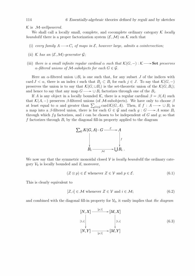
114 6 Essentially-algebraic theories defined by reguli and by sketches
K is M-wellpowered.We shall call a locally small, complete, and cocomplete ordinary category K locally
bounded if there is a proper factorization system (E ,M) on K such that
(i) every family A Ci of maps in E, however large, admits a cointersection;
(ii) K has an (E ,M)-generator G;
(iii) there is a small infinite regular cardinal α such that K(G,−) : K Set preservesα-filtered unions of M-subobjects for each G ∈ G.
Here an α-filtered union ∪Bi is one such that, for any subset J of the indices withcard J < α, there is an index i such that Bj ⊂ Bi for each j ∈ J . To say that K(G,−)preserves the union is to say that K(G,∪Bi) is the set-theoretic union of the K(G,Bi);and hence to say that any map G ∪ Bi factorizes through one of the Bi.
If A is any object in a locally bounded K, there is a regular cardinal β = β(A) suchthat K(A,−) preserves β-filtered unions (of M-subobjects). We have only to choose βat least equal to α and greater than
∑G∈G cardK(G,A). Then, if f : A ∪ Bi is
a map into a β-filtered union, there is for each G ∈ G and each g : G A some Bi
through which fg factorizes, and i can be chosen to be independent of G and g; so thatf factorizes through Bi by the diagonal fill-in property applied to the diagram
Bi
⋃Bi .M
∑G K(G,A) · G
Bi
∑G K(G,A) · G AE A
⋃Bi .
f
We now say that the symmetric monoidal closed V is locally bounded if the ordinary cate-gory V0 is locally bounded and if, moreover,
(Z ⊗ p) ∈ E whenever Z ∈ V and p ∈ E . (6.1)
This is clearly equivalent to
[Z, i] ∈ M whenever Z ∈ V and i ∈ M; (6.2)
and combined with the diagonal fill-in property for V0, it easily implies that the diagram
[N, Y ] [M,Y ][p,1]
[N,X]
[N, Y ]
[1,i]
[N,X] [M,X][p,1] [M,X]
[M,Y ]
[1,i]
(6.3)

6.2 The reflectivity in [Aop,V ] of the category of algebras for a regulus 115
is a pullback whenever p : M N is in E and i : X Y is in M. This “internal”version of the diagonal fill-in property is stronger than the original one, which we regainby applying the limit-preserving V : V0
Set to the pullback (6.3).
We now verify that all the examples of symmetric monoidal closed categories in 1.1are locally bounded. For the small preorders such as 2 and R+, all the conditions aretrivially satisfied with E = the epimorphisms, M = the extremal monomorphisms = theisomorphisms.
In the examples Set, Cat, Gpd, Ord, Shv S, Ab, R-Mod, G-R-Mod andDG-R-Mod, the category V0 is locally presentable in the sense of [31]; and any suchcategory K is locally bounded with E = the extremal epimorphisms, M = the monomor-phisms. For it is certainly E-cowellpowered, by Satz 7.14 of [31]; it has by definition astrong generator G, and this is an (E ,M)-generator by the remarks at the end of 3.4above; and there is by definition a regular α such that each K(G,−) : K Set forG ∈ G preserves α-filtered colimits – that is, each G ∈ G is α-presentable. Now, in thepresence of such a generator G, when ∪Bi is an α-filtered union of subobjects, the mapcolim Bi
∪Bi is a monomorphism, as pointed out in Lemma 3.2.1 of [30]; and hencein the present case is an isomorphism, for (lying in E) it is an extremal epimorphism.Thus in fact each K(G,−) preserves α-filtered unions. Finally, (6.2) is satisfied in eachof these examples, since the right-adjoint functor [Z,−] preserves monomorphisms. (Inall of these examples except Shv S, the category V0 is locally finitely presentable, inthe sense that, for a suitable choice of G, we may take α = ℵ0. Another account oflocally-presentable categories can be found in [45].)
In the topological examples CGTop, CGTop∗, HCGTop, and QTop, we take forM the subspace-inclusions and for E the surjections. The first three of these are easilyseen to be E-cowellpowered. The fourth is not – the two-point set admits a large set ofquasitopologies – yet it does admit all cointersections of surjections; we merely form thecointersection in Set and give it the appropriate quasitopology. The one-point space is ineach case an (E ,M)-generator, which satisfies (iii) with α = ℵ0. Moreover, (6.1) is clearlysatisfied, since the tensor product is the cartesian product – not only in V0, but also atthe level of the underlying sets.
For the final example Ban, we take E = the epimorphisms = the dense maps, M= the extremal monomorphisms = the inclusions of closed subspaces with the inducednorm. Cowellpoweredness is easy: if X Y is dense, Y can have no more pointsthan there are filters on the image of X. An (E ,M)-generator is G, where G is thebase-field R or C. It satisfies (iii) with α = ℵ1; for then an α-filtered union ∪Bi is theset-theoretical union. (In general ∪Bi is the closure of the set-theoretical union, so thatevery point of it is the limit of some sequence of the latter; when the union is ℵ1-filtered,the sequence lies entirely in some Bi.) Finally (6.2) is clearly satisfied, [Z, Y ] being theusual function-space.
6.2 The reflectivity in [Aop,V ] of the category of algebras for a regulus
The first step in making available the results of [44] is the proof of:

116 6 Essentially-algebraic theories defined by reguli and by sketches
Proposition 6.4 If V is locally bounded, so is the ordinary category [Aop,V ]0 for anysmall A.
Proof. Let (E ,M) be the proper factorization system on V0, and G the corresponding(E ,M)-generator. We define sets of maps in [Aop,V ]0, again called E and M, by decreeingthat a V-natural ρ : T S is to be in E or in M precisely when all of its componentsρA : TA SA are in the E or the M of V0. Clearly the new E and M contain theisomorphisms and are closed under composition. Since we test for a monomorphism as in3.3 by pulling it back along itself, and since small limits in [Aop,V ] are formed pointwise,the M of [Aop,V ]0 consists of monomorphisms; similarly the E consists of epimorphisms.
To see that every ρ : T S factorizes into an E and an M, we factorize eachcomponent ρA as
TA σA
RA τA
SA
with σA ∈ E and τA ∈ M. To make R into a V-functor Aop V , such that σ and τ areV-natural, we must so define RAB as to render commutative the top and left regions of
A(B,A) [TA, TB]TAB A(B,A)
[SA, SB]
SAB
A(B,A)
[RA,RB]
RAB
[SA, SB] [RA,SB][τA,1]
[RA,RB]
[RA,SB]
[1,τB ]
[RA,RB] [TA,RB][σA,1]
[RA,SB] [TA, SB][σA,1]
[TA, TB]
[TA,RB]
[1,σB ]
[TA,RB]
[TA, SB]
[1,τB ]
since the bottom right region is a pullback by (6.3), there is exactly one such map RAB –which is then easily seen to satisfy the axioms (1.5) and (1.6) for a V-functor.
To verify the diagonal fill-in property, let σ : T S be in E and let τ : P Q bein M. By (6.3) we have for each A ∈ A a pullback
[SA,QA] [TA,QA] ;[σA,1]
[SA, PA]
[SA,QA]
[1,τA]
[SA, PA] [TA, PA][σA,1] [TA, PA]
[TA,QA] ;
[1,τA]
applying∫
Ato this in accordance with (2.10), and recalling from (3.20) that limits com-
mute with limits, we get a corresponding pullback in which the top left corner is now[Aop,V ](S, P ); applying V : V0
Set to this, we get a pullback in Set expressingthe desired diagonal fill-in property. Hence (E ,M) is a proper factorization system on[Aop,V ]0.
Write H for the small set G ⊗A(−, A)G∈G,A∈A of objects of [Aop,V ]0. If R is aproper M-subobject of S, there is some A for which RA is a proper M-subobject of SA:
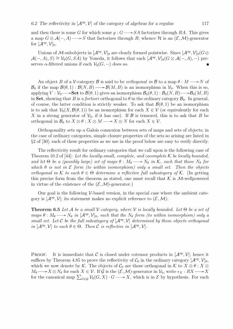
6.2 The reflectivity in [Aop,V ] of the category of algebras for a regulus 117
and then there is some G for which some g : G SA factorizes through RA. This givesa map G ⊗A(−, A) S that factorizes through R; whence H is an (E ,M)-generatorfor [Aop,V ]0.
Unions of M-subobjects in [Aop,V ]0 are clearly formed pointwise. Since [Aop,V ]0(G⊗A(−, A), S) ∼= V0(G,SA) by Yoneda, it follows that each [Aop,V ]0(G ⊗A(−, A),−) pre-serves α-filtered unions if each V0(G,−) does so.
An object B of a V-category B is said to be orthogonal in B to a map θ : M N ofB0 if the map B(θ, 1) : B(N,B) B(M,B) is an isomorphism in V0. When this is so,applying V : V0
Set to B(θ, 1) gives an isomorphism B0(θ, 1) : B0(N,B) B0(M,B)in Set, showing that B is a fortiori orthogonal to θ in the ordinary category B0. In general,of course, the latter condition is strictly weaker. To ask that B(θ, 1) be an isomorphismis to ask that V0(X,B(θ, 1)) be an isomorphism for each X ∈ V (or equivalently for eachX in a strong generator of V0, if it has one). If B is tensored, this is to ask that B beorthogonal in B0 to X ⊗ θ : X ⊗ M X ⊗ N for each X ∈ V.
Orthogonality sets up a Galois connexion between sets of maps and sets of objects; inthe case of ordinary categories, simple closure properties of the sets so arising are listed in§2 of [30]; such of these properties as we use in the proof below are easy to verify directly.
The reflectivity result for ordinary categories that we call upon is the following case ofTheorem 10.2 of [44]: Let the locally-small, complete, and cocomplete K be locally bounded,and let Θ be a (possibly large) set of maps θ : Mθ
Nθ in K, such that those Nθ forwhich θ is not in E form (to within isomorphism) only a small set. Then the objectsorthogonal in K to each θ ∈ Θ determine a reflective full subcategory of K. (In gettingthis precise form from the theorem as stated, one must recall that K is M-wellpoweredin virtue of the existence of the (E ,M)-generator.)
Our goal is the following V-based version, in the special case where the ambient cate-gory is [Aop,V ]; its statement makes no explicit reference to (E ,M):
Theorem 6.5 Let A be a small V-category, where V is locally bounded. Let Θ be a set ofmaps θ : Mθ
Nθ in [Aop,V ]0, such that the Nθ form (to within isomorphism) only asmall set. Let C be the full subcategory of [Aop,V ] determined by those objects orthogonalin [Aop,V ] to each θ ∈ Θ. Then C is reflective in [Aop,V ].
Proof. It is immediate that C is closed under cotensor products in [Aop,V ]; hence itsuffices by Theorem 4.85 to prove the reflectivity of C0 in the ordinary category [Aop,V ]0,which we now denote by K. The objects of C0 are those orthogonal in K to X ⊗ θ : X ⊗Mθ
X ⊗Nθ for each X ∈ V. If G is the (E ,M)-generator in V0, write εX : RX Xfor the canonical map
∑G∈G V0(G,X) · G X, which is in E by hypothesis. For each

118 6 Essentially-algebraic theories defined by reguli and by sketches
θ and each X, form the commutative diagram
X ⊗ Mθ P (X, θ)ρX,θ
RX ⊗ Mθ
X ⊗ Mθ
εX⊗Mθ
RX ⊗ Mθ RX ⊗ NθRX⊗θ RX ⊗ Nθ
P (X, θ)
σX,θ
X ⊗ Mθ
X ⊗ Nθ ,
X⊗θ
P (X, θ)
X ⊗ Nθ ,
τX,θ
RX ⊗ Nθ
X ⊗ Nθ ,
εX⊗Nθ
""
(6.6)
in which the top left region is a pushout. Since tensor products in [Aop,V ] are formedpointwise, it follows from (6.1) that εX ⊗ Nθ is in E , whence its factor τX,θ is in E .Every object orthogonal in K to RX ⊗ θ is also orthogonal to its pushout ρX,θ; it isthen orthogonal to the composite X ⊗ θ = τX,θρX,θ if and only if it is orthogonal to τX,θ.Thus C0 consists of the objects in K orthogonal to each RX ⊗ θ and to each τX,θ. SinceRX ⊗ θ = (
∑G V0(G,X) ·G)⊗ θ ∼=
∑G V0(G,X) · (G⊗ θ), any object orthogonal in K to
each G ⊗ θ is also orthogonal to the coproduct RX ⊗ θ of these; and thus C0 consists ofthe objects in K orthogonal to each G ⊗ θ for G ∈ G and to each τX,θ. Since the numberof different G⊗Nθ is small, and since each τX,θ is in E , the desired reflectivity of C0 in Kfollows from Proposition 6.4 and the result quoted before the theorem.
By Proposition 5.15, the cocomplete V-category C of Theorem 6.5 is the category ofalgebras for an essentially-algebraic theory K : A B, where K is the composite of theYoneda embedding A [Aop,V ] and the reflexion [Aop,V ] C. Clearly G : A Bis a comodel for the theory precisely when B(G−, B) : Aop V is for each B ∈ Borthogonal in [Aop,V ] to each θ ∈ Θ. By a very free adaptation of the terminology ofIsbell [37], we shall in future call such a set Θ as occurs in Theorem 6.5 a regulus . Weshall use such terms as Θ-comodel and K-comodel interchangeably, and shall write Θ-Algfor the category C of K-algebras.
6.3 The category of algebras for a sketch, and in particular for an F -theory; algebraic functors and their adjoints
We suppose henceforth that V is locally bounded. Let A be a small V-category, andconsider a set (not necessarily small)
Φ = φγ : FγA(Pγ−, Aγ)γ∈Γ (6.7)
of cylinders in A, where Fγ : Lopγ
V and Pγ : Lγ A, with each Lγ small. Call a
functor G : A B a Φ-comodel if, for each γ, the cylinder
Fγ φγ
A(Pγ−, Aγ) GB(GPγ−, GAγ) (6.8)

6.3 The category of algebras for a sketch 119
is a colimit-cylinder; and write Φ-Com[A,B] for the full subcategory of [A,B] given bythese comodels. Similarly, write Φ-Mod[Aop,P] for (Φ-Com[A,Pop])op, and write Φ-Algfor Φ-Mod[Aop,V ]. Thus the Φ-algebras are those Aop V that send each φγ to alimit-cone. By very freely adapting the terminology of Ehresmann [24] (see also [3]), wemay call the pair (Aop, Φ), or just Φ for short, a sketch.
Given such a sketch, each composite
Fγ φγ
A(Pγ−, Aγ) Y [Aop,V ](Y Pγ−, Y Aγ) (6.9)
corresponds by (3.5) to a map
θγ : Fγ Y PγY Aγ (6.10)
in the cocomplete [Aop,V ]. Write Θ = θγγ∈Γ for the set of these maps; because A issmall, the set of codomains in (6.10) is small, so that Θ is indeed a regulus in the senseof 6.2.
Theorem 6.11 If the regulus Θ corresponds as above to the sketch Φ, then
Φ-Com[A,B] = Θ-Com[A,B]
for any category B. In particular Φ-Alg is the reflective subcategory Θ-Alg of [Aop,V ]. Thecorresponding dense functor K : A Φ-Alg is fully faithful precisely when the cylindersφγ are already colimit-cylinders in A.
Proof. By the remarks at the end of 6.2, G : A B is a Θ-comodel precisely wheneach B(G−, B) is orthogonal in [Aop,V ] to each θγ; that is, when each
[Aop,V ](θγ , 1) : [Aop,V ](Y Aγ,B(G−, B)
) [Aop,V ]
(Fγ Y Pγ ,B(G−, B)
)is an isomorphism. By (3.5) and Yoneda, this map is isomorphic to a map
B(GAγ , B) [Lopγ ,V ]
(Fγ ,B(GPγ−, B)
), (6.12)
whose unit is easily verified to be (6.8); to say that it is an isomorphism is therefore by(3.5) to say that (6.8) is a colimit-cylinder, or that G is a Φ-comodel. Applying this tothe comodels in Vop gives by Theorem 5.59 the equality Φ-Alg = Θ-Alg.
By Proposition 5.16, K is fully faithful if and only if Φ-Alg contains the representablesA(−, A). To ask each A(−, A) to be an algebra is by (6.12) to ask that each
A(Aγ, A) [Lopγ ,V ]
(Fγ,A(Pγ−, A)
)be an isomorphism, and hence by (3.5) that each φγ be a colimit-cylinder.

120 6 Essentially-algebraic theories defined by reguli and by sketches
In particular, Φ-Alg is reflective in [Aop,V ] when Φ consists of all small colimit-cylinders in A; the reflectivity of V ′′
0 in V ′0 = [Vop
0 ,Set′] of 3.12 above is an example ofthis.
A very important special case of Theorem 6.11 is that where A is F -cocomplete forsome set F of small indexing-types, and where Φ consists of (the units of) all the F -colimits in A. In this case Φ-Com[A,B] = F - Cocts[A,B] and Φ-Alg = F -Cts[Aop,V ].The full name (Aop, Φ) of the sketch Φ might here be replaced by (Aop,F). It is alsosuggestive to refer to a small F -complete category Aop as an F -theory. For instance,with V = Set, a Lawvere-Benabou theory ([52], [7]) is a small category Aop with finiteproducts; while a small Aop with finite limits is sometimes called a finitary essentially-algebraic theory. (Joyal suggests calling the latter a cartesian theory ; in that finitelimits may be said to go back to Descartes, who introduced both the product R× R andthe equalizer (x, y) | f(x, y) = g(x, y).) This terminology moreover allows Aop-Alg (Fbeing understood) as a useful abbreviation for F -Cts[Aop,V ].
Consider now a sketch (Aop, Φ) where Φ is given by (6.7); let F be a set of smallindexing-types containing each Fγ occurring in Φ; and let B be a small F -cocompletecategory. Write K : A Φ-Alg and L : B Bop-Alg = F -Cts[Bop,V ] for the respectivedense functors, observing by Theorem 6.11 that L is fully faithful. Note that, since L isalso an L-comodel by (5.51), we have:
Proposition 6.13 For a small F-cocomplete B, the dense inclusion L : B Bop-Alg =F -Cts[Bop,V ] preserves and reflects F-colimits.
Consider a Φ-comodel G : A B. If Q : B D is any F -continuous functor,the composite QG is clearly another Φ-comodel. Taking D = Vop here, we see that[Gop, 1] : [Bop,V ] [Aop,V ] restricts to a functor
G : Bop-Alg Φ-Alg . (6.14)
Such a functor between the categories of algebras, induced by a realization (that is, amodel) Gop of one theory in the other, is often said to be algebraic: especially in the casewhere A too is F -cocomplete and Φ = (Aop,F).
Since L : Bop-Alg [Bop,V ] and K : Φ-Alg [Aop,V ] are fully faithful, since
[Gop, 1] : [Bop,V ] [Aop,V ]
has by Theorem 4.50 the left adjoint LanGop , and since L has by Theorem 4.51 the leftadjoint − L, it follows that the algebraic functor G has the left adjoint
G = (− L). LanGop .K : Bop-Alg Φ-Alg.
The value of this at P ∈ Bop-Alg is(LanGop(KP )
) L, which by (4.65) is also (KP ) (LG);
so that by (4.17) we have
G∼= LanK(LG). (6.15)
In fact G is recoverable from G. First observe that Proposition 6.13 gives:
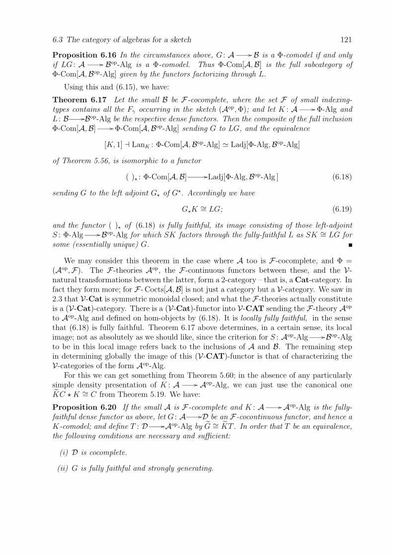
6.3 The category of algebras for a sketch 121
Proposition 6.16 In the circumstances above, G : A B is a Φ-comodel if and onlyif LG : A Bop-Alg is a Φ-comodel. Thus Φ-Com[A,B] is the full subcategory ofΦ-Com[A,Bop-Alg] given by the functors factorizing through L.
Using this and (6.15), we have:
Theorem 6.17 Let the small B be F-cocomplete, where the set F of small indexing-types contains all the Fγ occurring in the sketch (Aop, Φ); and let K : A Φ-Alg andL : B Bop-Alg be the respective dense functors. Then the composite of the full inclusionΦ-Com[A,B] Φ-Com[A,Bop-Alg] sending G to LG, and the equivalence
[K, 1] LanK : Φ-Com[A,Bop-Alg] Ladj[Φ-Alg,Bop-Alg]
of Theorem 5.56, is isomorphic to a functor
( ) : Φ-Com[A,B] Ladj[Φ-Alg,Bop-Alg ] (6.18)
sending G to the left adjoint G of G. Accordingly we have
GK ∼= LG; (6.19)
and the functor ( ) of (6.18) is fully faithful, its image consisting of those left-adjointS : Φ-Alg Bop-Alg for which SK factors through the fully-faithful L as SK ∼= LG forsome (essentially unique) G.
We may consider this theorem in the case where A too is F -cocomplete, and Φ =(Aop,F). The F -theories Aop, the F -continuous functors between these, and the V-natural transformations between the latter, form a 2-category – that is, a Cat-category. Infact they form more; for F - Cocts[A,B] is not just a category but a V-category. We saw in2.3 that V-Cat is symmetric monoidal closed; and what the F -theories actually constituteis a (V-Cat)-category. There is a (V-Cat)-functor into V-CAT sending the F -theory Aop
to Aop-Alg and defined on hom-objects by (6.18). It is locally fully faithful, in the sensethat (6.18) is fully faithful. Theorem 6.17 above determines, in a certain sense, its localimage; not as absolutely as we should like, since the criterion for S : Aop-Alg Bop-Algto be in this local image refers back to the inclusions of A and B. The remaining stepin determining globally the image of this (V-CAT)-functor is that of characterizing theV-categories of the form Aop-Alg.
For this we can get something from Theorem 5.60; in the absence of any particularlysimple density presentation of K : A Aop-Alg, we can just use the canonical oneKC K ∼= C from Theorem 5.19. We have:
Proposition 6.20 If the small A is F-cocomplete and K : A Aop-Alg is the fully-faithful dense functor as above, let G : A D be an F-cocontinuous functor, and hence aK-comodel; and define T : D Aop-Alg by G ∼= KT . In order that T be an equivalence,the following conditions are necessary and sufficient:
(i) D is cocomplete.
(ii) G is fully faithful and strongly generating.
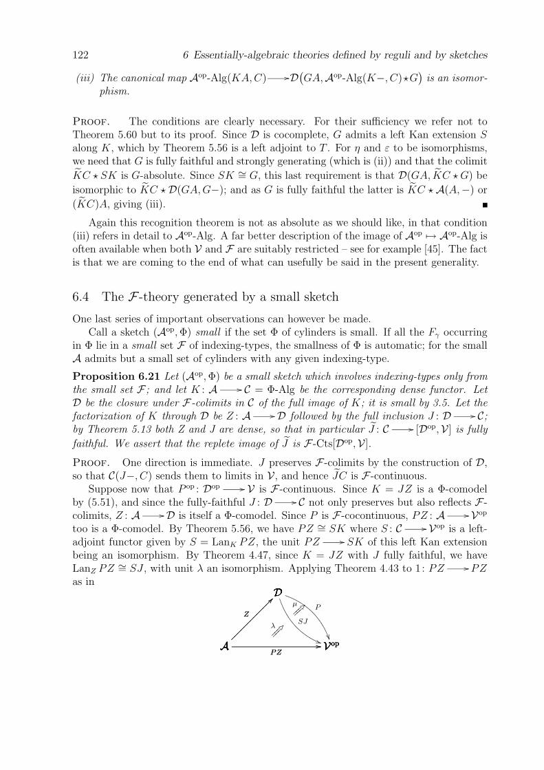
122 6 Essentially-algebraic theories defined by reguli and by sketches
(iii) The canonical map Aop-Alg(KA,C) D(GA,Aop-Alg(K−, C) G
)is an isomor-
phism.
Proof. The conditions are clearly necessary. For their sufficiency we refer not toTheorem 5.60 but to its proof. Since D is cocomplete, G admits a left Kan extension Salong K, which by Theorem 5.56 is a left adjoint to T . For η and ε to be isomorphisms,we need that G is fully faithful and strongly generating (which is (ii)) and that the colimit
KC SK is G-absolute. Since SK ∼= G, this last requirement is that D(GA, KC G) be
isomorphic to KC D(GA,G−); and as G is fully faithful the latter is KC A(A,−) or
(KC)A, giving (iii).
Again this recognition theorem is not as absolute as we should like, in that condition(iii) refers in detail to Aop-Alg. A far better description of the image of Aop → Aop-Alg isoften available when both V and F are suitably restricted – see for example [45]. The factis that we are coming to the end of what can usefully be said in the present generality.
6.4 The F -theory generated by a small sketch
One last series of important observations can however be made.Call a sketch (Aop, Φ) small if the set Φ of cylinders is small. If all the Fγ occurring
in Φ lie in a small set F of indexing-types, the smallness of Φ is automatic; for the smallA admits but a small set of cylinders with any given indexing-type.
Proposition 6.21 Let (Aop, Φ) be a small sketch which involves indexing-types only fromthe small set F ; and let K : A C = Φ-Alg be the corresponding dense functor. LetD be the closure under F-colimits in C of the full image of K; it is small by 3.5. Let thefactorization of K through D be Z : A D followed by the full inclusion J : D C;by Theorem 5.13 both Z and J are dense, so that in particular J : C [Dop,V ] is fully
faithful. We assert that the replete image of J is F -Cts[Dop,V ].
Proof. One direction is immediate. J preserves F -colimits by the construction of D,so that C(J−, C) sends them to limits in V , and hence JC is F -continuous.
Suppose now that P op : Dop V is F -continuous. Since K = JZ is a Φ-comodelby (5.51), and since the fully-faithful J : D C not only preserves but also reflects F -colimits, Z : A D is itself a Φ-comodel. Since P is F -cocontinuous, PZ : A Vop
too is a Φ-comodel. By Theorem 5.56, we have PZ ∼= SK where S : C Vop is a left-adjoint functor given by S = LanK PZ, the unit PZ SK of this left Kan extensionbeing an isomorphism. By Theorem 4.47, since K = JZ with J fully faithful, we haveLanZ PZ ∼= SJ , with unit λ an isomorphism. Applying Theorem 4.43 to 1: PZ PZas in
A VopPZ
D
A
Z
D
Vop
P
A Vop
PZ
D
A
Z
D
Vop
SJ
λ
µ #
6.4 The F -theory generated by a small sketch 123
gives a map µ : SJ P with µZ an isomorphism. Since both P and SJ preserve F -colimits, and since D is the closure under F -colimits of the full image of Z (which is thefull image of K), we conclude that µ : SJ P is an isomorphism.
The right-adjoint Sop : Cop V being necessarily a representable C(−, C), we have
P op ∼= SopJop ∼= C(J−, C) = JC, as required.
Now Theorem 6.11 gives:
Corollary 6.22 In these circumstances the functor J is isomorphic to the inclusionD Dop-Alg of the F-cocomplete small D, so that for any B we have J-Com[D,B] =F - Cocts[D,B].
Since the size of F here is bounded only below by the knowledge of the sketch Φ, wecannot expect the comodels of the sketches (Aop, Φ) and (Dop,F) to “coincide” in everyB; that they do so when B is F -cocomplete is an example of the “sufficient completeness”referred to in the penultimate paragraph of 5.13. The precise result is:
Theorem 6.23 In the circumstances of Proposition 6.21, every Φ-comodel G : A Badmits a left Kan extension along Z : A D whenever B is F-cocomplete; and we havean equivalence
LanZ [Z, 1] : F - Cocts[D,B] Φ-Com[A,B]
whose unit and counit are the canonical maps.
Proof. By Corollary 6.22 and Theorem 5.52, we have only to show that every Φ-comodelG : A B has the form HZ for some F -continuous H : D B.
We suppose first that B is small, and consider the inclusion L : B Bop-Alg ofProposition 6.13. Then LG, being itself a Φ-comodel as in Proposition 6.16, is by The-orem 5.56 isomorphic to SK for some left-adjoint S : Φ-Alg Bop-Alg; in fact S isthe G of (6.19). The set H of those objects C ∈ C for which SC lies in B ⊂ Bop-Algcertainly contains all the objects KA, since SK ∼= LG; and it is closed under F -colimitsby Proposition 6.13, since the left-adjoint S preserves colimits; hence H contains D bythe definition of this latter. Thus SJ ∼= LH for some H : D B, which is clearly F -cocontinuous since SJ is so. Now LG ∼= SK = SJZ ∼= LHZ; and (L being fully faithful)we have the desired result G ∼= HZ.
Passing to the case where the F -cocomplete B need not be small, let B′ be the closureunder F -colimits in B of the full image of the Φ-comodel G : A B; this latter factorizingas G′ : A B′ followed by the full inclusion N : B′ B. Since N preserves andreflects F -colimits, G′ is itself a Φ-comodel; and since B′ is small by 3.5, we have as aboveG′ ∼= H ′Z for some F -cocontinuous H ′ : D B′. Now G ∼= HZ, where H = NH ′ isF -cocontinuous.
We may say that Dop is the F-theory generated by the sketch (Aop, Φ), or that (Aop, Φ)is a sketch of the F-theory Dop. The latter form of words comes closer to explicatingEhresmann’s choice of the word “sketch”. As he used the word (in the case V = Set),the small category A was not in general explicitly given, but presented by generators andrelations; often this presentation was finite, and Φ was a finite set of finite cones (thecolimits involved in F classically being conical ones). In such cases, one can literally see

124 6 Essentially-algebraic theories defined by reguli and by sketches
(the presentation of) (Aop, Φ) as a finitary way of “sketching” the generally infinite andcomplicated structure of Dop, or the still more complicated structure of Dop-Alg.
When V = Set and F consists of the functors ∆1: L Set for finite L, the F -theories are the cartesian theories of 6.3 above; the sketch (Aop, Φ) gives rise to such atheory if Φ is a small set of finite cones. It is exactly the categories Φ-Alg for such a Φthat are the locally finitely presentable categories; D ⊂ Φ-Alg is a small dense subcategorycomposed of objects which (since finite limits commute with filtered colimits in Set) arefinitely presentable. In all the examples of categories V0 that we declared locally finitelypresentable in 6.1, it is easy to see that V0 = Φ-Alg for such a sketch Φ. For furtherinformation on the relation of locally presentable categories to reguli and sketches, seethe classical [31], or the newer [45] which extends the ideas to certain important V otherthan Set. These V include Cat and Gpd, which are the appropriate base categoriesfor the study of categories with essentially-algebraic structure. At this level, as is wellknown, equivalence becomes more central than isomorphism, and the naturally-occurring“functors” and “transformations” are more general than the V-functors and the V-naturaltransformations; which leads to various problems of coherence. The study of essentially-algebraic theories in this context must take account of these more general notions; this isnot touched on in [45], but a beginning is made in [46].
6.5 The symmetric monoidal closed structure on the category of F -cocomplete categories and F -cocontinuous functors
Before ending, we give a final application of Theorem 6.23. We consider the (V-Cat)-category of small F -cocomplete categories A, where F is a small set of indexing-types.Since F - Cocts[A,B] denotes the (V-Cat)-valued hom here, an appropriate name for thiscategory is F - Cocts.
If B and C are F -cocomplete, so of course is [B, C], with F -colimits formed pointwise.The full subcategory F - Cocts[B, C] of this is again F -cocomplete, since colimits commutewith colimits. The functors Q : A F - Cocts[B, C] correspond to those functors P : A⊗B C for which each partial functor P (A,−) : B C is F -cocontinuous. If A toois F -cocomplete, the functor Q is itself F -cocontinuous precisely when the other partialfunctors P (−, B) : A C are also F -cocontinuous. We are thus led to the notion of aP : A⊗ B C which is F -cocontinuous in each variable separately.
Such a P is a comodel for a sketch((A⊗B)op, Φ
). If λ : F A(T−,M) is a cylinder
in A, where F : Lop V and T : L A, we can consider for B ∈ B the functor
L ∼= L ⊗ IT⊗B
A⊗ B
sending L to (TL,B), and called T ⊗ B. Then we can consider the cylinder
Fλ
A(T−,M) ∼= A(T−,M)⊗I1⊗j
A(T−,M)⊗B(B,B) = (A⊗B)((T−, B), (M,B)
),
and call this λ⊗B. Note that this is a colimit-cylinder in A⊗B if λ is one in A; essentiallybecause −⊗ Y : V V preserves colimits. If we take Φ to consist of all the λ⊗ B and

6.5 Symmetric monoidal closed structure on F -cocomplete categories 125
all the A ⊗ µ, where λ is an F -colimit-cylinder in A and µ is an F -colimit-cylinder in B,the Φ-comodels P : A ⊗ B C are precisely those P that are F -cocontinuous in eachvariable. In fact more than this is true; it is easy to see that
Φ-Com[A⊗ B, C] ∼= F - Cocts[A,F - Cocts[B, C]
].
Write (A ⊗F B)op for the F -theory generated by the sketch((A ⊗ B)op, Φ
). In view of
Theorem 6.23 we get
F - Cocts[A⊗F B, C] F - Cocts[A,F - Cocts[B, C]
]. (6.24)
The symmetry in A, B, C of F - Cocts[A,F - Cocts[B,F - Cocts[C,D]]
]now easily gives
(A⊗F B) ⊗F C A⊗F (B ⊗F C) (6.25)
andA⊗F B B ⊗F A. (6.26)
If A is the free F -cocompletion of A as in Theorem 5.35, it is clear that (for any small Aand B)
A⊗F B A⊗ B ; (6.27)
it is also clear that, for any small A and for F -cocomplete B, the F -cocontinuous functorsA ⊗F B C correspond to the functors P : A ⊗ B C for which P (A,−) is F -cocontinuous. It follows that
I ⊗F B B , (6.28)
where I is the free F -cocompletion of I; which by Theorem 5.35 is the closure of I in Vunder F -colimits.
The coherence, in the appropriate sense, of the maps (6.25), (6.26), and (6.28), followsfrom the universal property (6.24). Thus the (V-Cat)-category F - Cocts is endowed withsomething like a symmetric monoidal closed structure – the difference being that we haveequivalences in place of isomorphisms.

126 6 Essentially-algebraic theories defined by reguli and by sketches
Bibliography
[1] C. Auderset, Adjonctions et monades au niveau des 2-categories, Cahiers de Top. etGeom. Diff. 15(1974), 3-20.
[2] H. Bass, Algebraic K-theory, W.A. Benjamin Inc., New York and Amsterdam, 1968.
[3] A. Bastiani and C. Ehresmann, Categories of sketched structures, Cahiers de Top.et Geom. Diff. 13(1972), 103-214.
[4] J. Benabou, Categories avec multiplication, C.R. Acad. Sci. Paris 256(1963), 1887-1890.
[5] J. Benabou, Categories relatives, C.R. Acad. Sci. Paris 260(1965), 3824-3827.
[6] J. Benabou, Introduction to bicategories, Lecture Notes in Math. 47(1967), 1-77.
[7] J. Benabou, Structures algebriques dans les categories, Cahiers de Top. et Geom.Diff. 10 (1968), 1-126.
[8] J. Benabou, Les distributeurs, Univ. Cath. de Louvain, Seminaires de Math. Pure,Rapport No. 33(1973).
[9] F. Borceux and G.M. Kelly, A notion of limit for enriched categories, Bull. Austral.Math. Soc. 12(1975), 49-72.
[10] M. Bunge, Relative functor categories and categories of algebras, J. Algebra 11(1969),64-101.
[11] E. Brown, Cohomology theories, Ann. Math. 75(1962), 467-484.
[12] B.J. Day, On closed categories of functors, Lecture Notes in Math. 137(1970), 1-38.
[13] B.J. Day, Construction of biclosed categories (Ph.D. Thesis, University of New SouthWales, 1970).
[14] B.J. Day, A reflection theorem for closed categories, J. Pure Appl. Algebra 2(1972),1-11.
[15] B.J. Day, On adjoint-functor factorization, Lecture Notes in Math. 420(1974), 1-19.
[16] B.J. Day, On closed categories of functors II, Lecture Notes in Math. 420(1974), 20-54.
127

128 BIBLIOGRAPHY
[17] B.J. Day, An embedding theorem for closed categories, Lecture Notes in Math.420(1974), 55-64.
[18] B.J. Day, An adjoint-functor theorem over topoi, Bull. Austral. Math. Soc. 15(1976),381-394.
[19] B.J. Day and G.M. Kelly, On topological quotient maps preserved by pullbacks orproducts, Proc. Cambridge Phil. Soc. 67(1970), 553-558.
[20] B.J. Day and G.M. Kelly, Enriched functor categories, Lecture Notes in Math.106(1969), 178-191.
[21] Y. Diers, Type de densite d’une sous-categorie pleine, Ann. Soc. Scient. Bruxelles90(1976), 25-47.
[22] E.J. Dubuc, Kan extensions in enriched category theory, = Lecture Notes in Math.145(1970).
[23] E. J. Dubuc and H. Porta, Convenient categories of topological algebras, and theirduality theory, J. Pure Appl. Algebra 3(1971), 281-316.
[24] C. Ehresmann, Esquisses et types de structures algegriques, Bul. Inst. Polit. Iasi14(1968), 1-14.
[25] S. Eilenberg and G.M. Kelly, A generalization of the functorial calculus, J. Algebra3(1966), 366-375.
[26] S. Eilenberg and G.M. Kelly, Closed categories, Proc. Conf. on Categorical Algebra(La Jolla, 1965), Springer-Verlag, Berlin-Heidelberg-New York, 1966; 421-562.
[27] J. Fisher-Palmquist and P.H. Palmquist, Morita contexts of enriched categories, Proc.Amer. Math. Soc. 50(1975), 55-60.
[28] P.J. Freyd, Abelian categories: an introduction to the theory of functors, Harper andRow, New York, Evanston, and London, 1964. Available as TAC Reprints number 3,http://www.emis.de/journals/TAC/reprints/articles/3/tr3abs.html
[29] P.J. Freyd, Several new concepts: lucid and concordant functors, pre-limits, pre-completeness, the continuous and concordant completions of categories, Lecture Notesin Math. 99(1969), 196-241.
[30] P.J. Freyd and G.M. Kelly, Categories of continuous functors I, J. Pure Appl. Algebra2(1972), 169-191; Erratum, J. Pure Appl. Algebra 4(1974), 121.
[31] P. Gabriel and F. Ulmer, Lokal prasentierbare Kategorien, = Lecture Notes in Math.221(1971).
[32] J.W. Gray, Closed categories, lax limits and homotopy limits, J. Pure Appl. Algebra19(1980), 127-158.
BIBLIOGRAPHY 129
[33] M.F. Gouzou and R. Grunig, U -distributeurs et categories de modules, Manuscript,Univ. de Paris, 7, 1975.
[34] A. Grothendieck, Categories fibrees et descente, Seminaire de geometrie algebriquede l’I.H.E.S., Paris, 1961.
[35] J.R. Isbell, Adequate subcategories, Illinois J. Math. 4(1960), 541-552.
[36] J.R. Isbell, Structure of categories, Bull. Amer. Math. Soc. 72(1966), 619-655.
[37] J.R. Isbell, General functorial semantics I, Amer. J. Math. 94(1972), 535-596.
[38] D.N. Kan, Adjoint functors, Trans. Amer. Math. Soc. 87(1958), 294-329.
[39] G.M. Kelly, On Mac Lane’s conditions for coherence of natural associativities, com-mutativities, etc., J. Algebra 1(1964), 397-402.
[40] G.M. Kelly, Tensor products in categories, J. Algebra 2(1965), 15-37.
[41] G.M. Kelly, Monomorphisms, epimorphisms, and pull-backs, J. Austral. Math. Soc.9(1969), 124-142.
[42] G.M. Kelly, Adjunction for enriched categories, Lecture Notes in Math. 420(1969),166-177.
[43] G.M. Kelly, Doctrinal adjunction, Lecture Notes in Math. 420(1974), 257-280.
[44] G.M. Kelly, A unified treatment of transfinite constructions for free algebras, freemonoids, colimits, associated sheaves, and so on, Bull. Austral. Math. Soc. 22(1980),1-83.
[45] G.M. Kelly, Structures defined by finite limits in the enriched context. I. Third Col-loquium on Categories, Part VI (Amiens, 1980). Cahiers Topologie Geom. 23 (1982),3–42.
[46] G.M. Kelly, Categories with structure – biadjoints for algebraic functors, to appear.
[47] G.M. Kelly and S. Mac Lane, Coherence in closed categories, J. Pure Appl. Algebra1(1971), 97-140; Erratum, J. Pure Appl. Algebra 1(1971), 219.
[48] G.M. Kelly and S. Mac Lane, Closed coherence for a natural transformation, LectureNotes in Math. 281(1972), 1-28.
[49] G.M. Kelly and R.H. Street, Review of the elements of 2-categories, Lecture Notesin Math. 420(1974), 75-103.
[50] J.F. Kennison, On limit-preserving functors, Illinois J. Math. 12(1968), 616-619.
[51] A. Kock, Closed categories generated by commutative monads, J. Austral. Math.Soc. 12(1971), 405-424.

130 BIBLIOGRAPHY
[52] F.W. Lawvere, Functorial semantics of algebraic theories, Proc. Nat. Acad. Sci.U.S.A. 50(1963), 869-872.
[53] F.W. Lawvere, Teoria delle categorie sopra un topos di base, Mimeographed notes,Perugia 1972/1973.
[54] F.W. Lawvere, Metric spaces, generalized logic, and closed categories, Rend. del Sem.Mat. e Fis. di Milano, 43(1973), 135-166. Available as TAC Reprints number 1,http://www.emis.de/journals/TAC/reprints/articles/1/tr1abs.html
[55] H. Lindner, Morita equivalences of enriched categories. Cahiers de Top. et Geom.Diff. 15(1974), 377-397.
[56] F.E.J. Linton, Autonomous categories and duality of functors, J. Algebra 2(1965),315-349; Erratum, J. Algebra 4(1966), 172.
[57] F.E.J. Linton, Relative functorial semantics: adjointness results, Lecture Notes inMath. 99(1969), 384-418.
[58] S. Mac Lane, Natural associativity and commutativity, Rice Univ. Studies 49(1963),28-46.
[59] S. Mac Lane, Categorical algebra, Bull. Amer. Math. Soc. 71(1965), 40-106.
[60] S. Mac Lane, Categories for the Working Mathematician, Springer-Verlag, New York-Heidelberg-Berlin, 1971.
[61] J.P. May, The geometry of iterated loop spaces, Lecture Notes in Math. 271(1972).
[62] J.P May, Pairings of categories and specta, J. Pure Appl. Algebra 19(1980), 299-346.
[63] B. Mitchell, Low dimensional group cohomology as monoidal structures, Amer. J.Math. 105 (1983), 1049–1066.
[64] Ju. A. Mitropol’skii and L.A. Nazorova, editors: Matrix Problems, Akad. NaukUkrain, SSR Inst. Mat., Kiev, 1977. (in Russian)
[65] K. Morita, Duality for modules and its application to the theory of rings with mini-mum condition, Sci. Rep. Tokoyo Kyoiku Daigaku, Sect. A, 6(1958), 83-142.
[66] D. Newell, Morita theorems for functor categories, Trans. Amer. Math. Soc.168(1972), 423-434.
[67] J. Wick Pelletier, Dual functors and the Radon-Nikodym property in the category ofBanach spaces, J. Austral. Math. Soc. (Series A) 27(1979), 479-494.
[68] S.V. Polin, Morita equivalence and the Jacobson-Rees theorems for rings and monoidsin closed categories, Soviet Math. Doklady 15(1974), 1248-1251.
[69] E. Spanier, Quasi-topologies, Duke Math. J. 30(1963), 1-14.

BIBLIOGRAPHY 131
[70] R.H. Street, The formal theory of monads, J. Pure Appl. Algebra 2(1972), 149-168.
[71] R.H. Street, Fibrations and Yoneda’s lemma in a 2-category, Lecture Notes in Math.420(1974), 104-133.
[72] R.H. Street, Elementary cosmoi I, Lecture Notes in Math. 420(1974), 134-180.
[73] R.H. Steet, extract from a letter to F. Foltz; to appear in Diagrammes.
[74] R.H. Street and R.F.C. Walters, The comprehensive factorization of a functor, Bull.Amer. Math. Soc. 79(1973), 936-941.
[75] R.F.C. Walters, Sheaves and Cauchy-complete categories, Third Colloquium on Cat-egories, Part IV (Amiens, 1980). Cahiers Topologie Geom. Diff. 22 (1981), 283–286.
[76] R.F.C. Walters, Sheaves on sites as Cauchy-complete categories. J. Pure Appl. Alge-bra 24 (1982), 95–102.

Index
Absolute colimit, 101K-absolute colimit, 92
Accessible functor, 77weakly accessible functor, 78
Adequate, 86adjoint
partial, 24Adjoint functor theorem
general, 79special, 80
Adjoint, left, 23Adjoint, right, 23Adjunction, 24Algebra, 109, 119
for a regulus, 118for a sketch, 119
Algebraic functor, 120Atom, 80
Bicategory, 4Biclosed
bicategory, 14monoidal category, 14
Boolean algebra, 15
C-object in P, 109C-object in P , 109Cartesian theory, 120Category
2-category, 8cartesian closed, 14cartesian monoidal, 7closed, 14enriched over V , 8filtered, 71finite, 71functor category, 30
monoidal, 7monoidal biclosed, 14monoidal closed, 14of elements of F , 22underlying, 10
Cauchy complete, 95Cauchy completion, 95Closed, 7Closed monoidal category, 14Closure
under a family of colimits, 45, 82under a family of cylinders, 82
Cocomplete, 27F -cocomplete, 99finitely, 71
Cocompletion, free, 67Cocontinuous, 39, 99
F -cocontinuous, 99Codense, 86Coend, 53Cogenerator, strong, 46Coherence, 124Coherence axioms, 7, 11, 12Cointersection, 113Colimit
absolute, 101classical, 42conical, 42, 50, 52F -colimits, 99filtered, 72indexed, 38iterated, 51K-absolute, 92pointwise, 40
Comodel, 106for a regulus, 118
132
INDEX 133
for a sketch, 119Complete, 27, 50
finitely, 71Completion
Cauchy, 95idempotent-splitting, 100under F -colimits, 100under finite colimits, 101
Componentconnected, 44
Componentsof a V-natural transformation, 9
Composition law, 8Comprehensive factorization system, 73Cone, 42
canonical inductive, 43projective, 42
Conical limit or colimitclassical, 42in a V-category, 49, 50, 52
Connected component, 44Conservative, 8, 46Continuity of a limit in its index, 42Continuous, 39Contravariant functor, 13
representable, 16Copower, 48Cotensor product, 48Cotensored, 48Counit
of a general end, 52of a limit, 37of a representation, 22of a right Kan extension, 60of an adjunction, 23of an end in V , 27
Cowellpoweredness, weak, 47Cylinder, 38, 118–120, 122, 124
K-cylinder, 81
Dense, 86Dense functors, 119–122
composition of, 87Density presentation, 121
Density, formulations for, 85Diagonal fill-in, 113Diagram, 37Directed, 72Discrete Grothendieck construction, 74Discrete op-fibration, 73Distributor, 95Dual V-category, 12
(E ,M)-generator, 113Element
of X ∈ V, 8of a set-valued functor, 29
Endin V , 27in any V-category, 52
Epimorphism, extremal, 44Equivalence, 24Essentially surjective, 24Essentially-algebraic
structure, 124theory, 107, 109, 124
finitary, 120Extraordinary V-naturality, 18Extremal epimorphism, 44
F -cocomplete, 99F -Cocontinuous, 99F -colimits, 99F -theory, 120
generated by a sketch, 123, 125Factorization system, 74
comprehensive, 73proper, 113
Filtered category, 71α-filtered, 73
Filtered colimit, 72Filtered-colimit completion, 102Final diagram, 70Final functor, 70Finitary essentially-algebraic theory, 120Finite-colimit completion, 101Finitely complete, 71Finitely presentable, 83Finitely cocomplete, 71

134 INDEX
Flat, 102Free cocompletion, 67Fubini theorem
general, 41Full image, 25Full subcategory, 9Fully faithful
locally, 121Fully faithfulfunctor, 9Functor
2-functor, 10algebraic, 120conservative, 8contravariant, 13contravariant representable, 16enriched over V , 9flat, 102fully faithful, 9generating, 46of two variables, 13partial, 13representable, 16, 22underlying, 10
Functor category, 30
General adjoint functor theorem, 79Generating functor, 46Generator, 46
(E ,M)-generator, 113regular, 81strong, 46
Generic model, 109Grothendieck construction
discrete, 74
Heyting algebra, 15Hom, internal, 14
Idempotent monad, 25Idempotent, split, 100Idempotent-splitting completion, 100Identity element, 8Image
full, 25replete, 25
Indexed colimit, 38Indexed limit, 37Indexing type, 37Inductive cone, canonical, 43Initial diagram, 69Initial functor, 70Interchange
of ends in V , 29of limits in general, 41
Interesction of subobjects, 80Internal hom, 14Intersection of subobjects
of M-subobjects, 113Iterated colimit, 51
K-absolute colimit, 92K-comodel, 106K-cylinder, 81K-model, 107Kan adjoint, 67Kan extension, 60, 61
pointwise, 65weak, 65
Left adequate, 86Left adjoint, 23Left exact, 71Left Kan extension, 61
weak, 65Limit
classical, 42conical, 42, 49, 52indexed, 37pointwise, 40
Limit cone, 42, 49Locally bounded, 114, 118Locally finitely presentable, 115, 124Locally fully faithful, 121Locally presentable, 115Locally small, 8, 10
M-subobject, 113M-wellpowered, 114Mates, 25Model, 107

INDEX 135
for a regulus, 118for a sketch, 119generic, 109
Monad, idempotent, 25Monoidal category, 7
biclosed, 14cartesian, 7closed, 14strict, 8symmetric, 12
Morita equivalence, 95
Opposite V-category, 12Orthogonal, 117, 119
Partial adjoint, 24Partial functor, 13Pointwise Kan extension, 65Pointwise limit or colimit, 40Pointwise limits, preservation of, 42Power, 48Presentation of density, 93Preservation
of a limit, 39of a right Kan extension, 60
Profunctors, 95Projective cone, 42Proper factorization system, 113
Realization, 120Reflect limits, 44Reflective full subcategory, 25Regular generator, 81Regulus, 118, 119Replete full subcategory, 25Replete image, 25Repletion, 25Representable V-functor, 16, 22Representation, 22Right adequate, 86Right adjoint, 23Right exact, 71Right Kan extension, 60
Sketch, 119, 123
of an F -theory, 123small, 122
Small, 10, 33Small limit
α-small, 73Small-projective, 94Small sketch, 122Small V-category, 9, 27Solution-set condition, 79Special Adjoint Functor Theorem, 80Split coequalizer diagram, 81Split idempotent, 100Strict monoidal category, 8Strong cogenerator, strongly cogenerat-
ing, 46Strong generator, strongly generating, 46,
121Subobject, 80
M-subobject, 113Surjective, essentially, (on objects), 24Symmetric, 7Symmetric monoidal category, 12Symmetry, 11
Tensor product, 8, 48of F -theories, 124of V-theories, 12
Tensored, 48Theory, cartesian, 120Theory, essentially-algebraic, 107, 109
F -theory, 120finitary, 120
Transformation, V-natural, 9Triangular equations, 23
Underlying category, 10Underlying functor, 10Union, of M-subobjects, 113Unit object, 8Unit of a(n)
adjunction, 23colimit, 38left Kan extension, 61representation, 22
Unit V-category, 10

136 INDEX
Universal V-natural family, 27
V-category, 8cocomplete, 39complete, 39dual, 12opposite, 12small, 9, 27unit, 10
V-functor, 9accessible, 77cocontinuous, 39conservative, 46continuous, 39dense, 86representable, 16, 22strongly cogenerating, 46strongly generating, 46
V-natural familyextraordinary, 18universal, 27
V-natural transformation, 9
Weak Kan extension, 65Weakly accessible, 78Weakly cowellpowered, 47Wellpowered: M-wellpowered, 114
Yoneda embedding, 34Yoneda isomorphism, 33, 39Yoneda lemma
strong, 33weak, 21

REPRINTS IN THEORY AND APPLICATIONS OF CATEGORIES will disseminate articles from thebody of important literature in Category Theory and closely related subjects which have never beenpublished in journal form, or which have been published in journals whose narrow circulation makes accessvery difficult. Publication in ‘Reprints in Theory and Applications of Categories’ will permit free and fulldissemination of such documents over the Internet. Articles appearing have been critically reviewed bythe Editorial Board of Theory and Applications of Categories. Only articles of lasting significance areconsidered for publication. Distribution is via the Internet tools WWW/ftp.
Subscription information Individual subscribers receive (by e-mail) abstracts of articles asthey are published. To subscribe, send e-mail to [email protected] including a full name and postal address.For institutional subscription, send enquiries to the Managing Editor.
Selection of reprints After obtaining written permission from any copyright holder, anythree TAC Editors may propose a work for TAC Reprints to the Managing Editor. The proposal willbe reported to all Editors. The Managing Editor may either accept the proposal or require that theEditors vote on it. Before such a vote, the author, title and original publication data will be circulatedto Editors. If a 2/3 majority of those TAC Editors responding within one month agrees, the work willbe accepted for TAC Reprints. After a work is accepted, the author or proposer must provide to TACeither a usable TeX source or a PDF document acceptable to the Managing Editor that reproduces atypeset version. Up to five pages of corrections, commentary and forward pointers may be appended bythe author. When submitting commentary, authors should read and follow the Format for submission ofTheory and Applications of Categories at http://www.tac.mta.ca/tac/.
Managing editor Robert Rosebrugh, Mount Allison University: [email protected]
TEXnical editor Michael Barr, McGill University: [email protected]
Transmitting editors
Richard Blute, Universite d’ Ottawa: [email protected] Breen, Universite de Paris 13: [email protected] Brown, University of North Wales: [email protected] Brylinski, Pennsylvania State University: [email protected] Carboni, Universita dell Insubria: [email protected] de Paiva, Xerox Palo Alto Research Center: [email protected] Getzler, Northwestern University: getzler(at)math(dot)northwestern(dot)eduMartin Hyland, University of Cambridge: [email protected]. T. Johnstone, University of Cambridge: [email protected]. Max Kelly, University of Sydney: [email protected] Kock, University of Aarhus: [email protected] Lack, University of Western Sydney: [email protected]. William Lawvere, State University of New York at Buffalo: [email protected] Loday, Universite de Strasbourg: [email protected] Moerdijk, University of Utrecht: [email protected] Niefield, Union College: [email protected] Pare, Dalhousie University: [email protected] Rosicky, Masaryk University: [email protected] Shipley, University of Illinois at Chicago: [email protected] Stasheff, University of North Carolina: [email protected] Street, Macquarie University: [email protected] Tholen, York University: [email protected] Tierney, Rutgers University: [email protected] F. C. Walters, University of Insubria: [email protected]. J. Wood, Dalhousie University: [email protected]