Turbulent Flow through a Nozzle Tutorial

Appendix E

Introduction………………………………………………pg.2

Geometry Creation……..……………………………………………pg.3

Mesh Creation……………………………………………pg.14

Abstract…………...……………………………...………pg.20

Problem Statement………..………….……………………………pg.20

Problem Setup……….……………………………………….…….pg.24

Solution…………...………………………………..…….pg.29

Results……………………………………………….…..pg.32

Validation……...…………………………………………pg 37

Summary…………………………………………….…..pg.39

1 | P a g e

Nozzle tutorial

Meshing Tutorial—Nozzle

Introduction: The purpose of this tutorial is to introduce new users to the fundamentals of creating the geometry and corresponding mesh for a nozzle. Specifically this tutorial showcases more aspect of using ANSYS Workbench not touched upon in the previous Meshing Tutorials (Laminar Pipe Flow, Turbulent Pipe Flow, Laminar Flow over a Flat Plate).

Problem Statement:

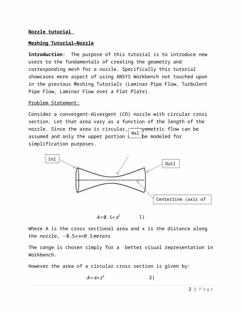
Consider a convergent-divergent (CD) nozzle with circular cross section. Let that area vary as a function of the length of the nozzle. Since the area is circular, axisymmetric flow can be assumed and only the upper portion will be modeled for simplification purposes.

A=0.1+x2 1)

Where A is the cross sectional area and x is the distance along the nozzle, −0.5<x<0.5meters

The range is chosen simply for a better visual representation in Workbench.

However the area of a circular cross section is given by:

A=π∗r2 2)

∴π∗r2=0.1+x2

Solving for the radius, a relationship can be obtained for the radius as a function of the distance along the nozzle:

r=√ 0.1+x2

π 3)

The equation is to be used later in Excel to obtain the data points necessary for the curved portion of the nozzle.

2 | P a g e

Outlet

Centerline (axis of symmetry)

Wall

Inlet

Nozzle—Geometry:

Open ANSYS Workbench, and by default a new project is started. Under Toolbox, drag the Mesh Component System onto the Project Schematic. Rename the system Nozzle.

o We are to model a 2d geometry therefore right click Geometry and select Properties.

o Under Advanced Geometry Options, next to Analysis Type, specify 2d.

Figure 1. N

Double click Geometry.

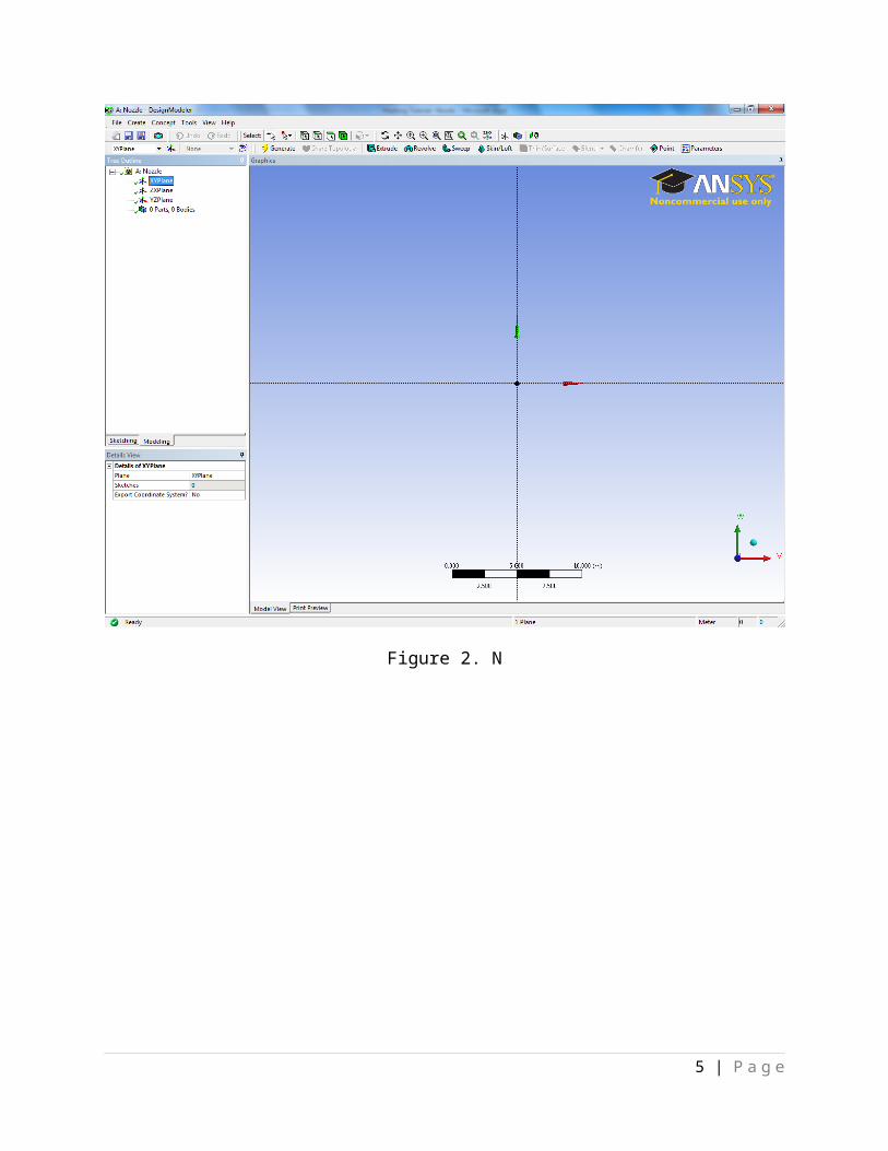
In the DesignModeler keep the default length units of meters. Manipulate the plane in order to obtain a 2d view in the graphics window—click on the

x-axis in the triad visible in the lower right hand portion of the graphics window.o If the triad is not visible, it can be accessed from Main Menu—View and then

select Triad. Under Tree Outline select the XYPlane.

3 | P a g e

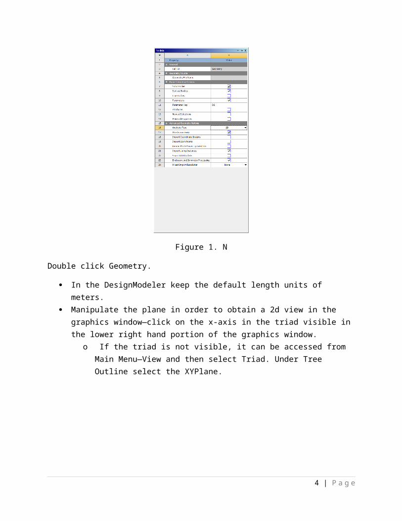
Figure 2. N

4 | P a g e

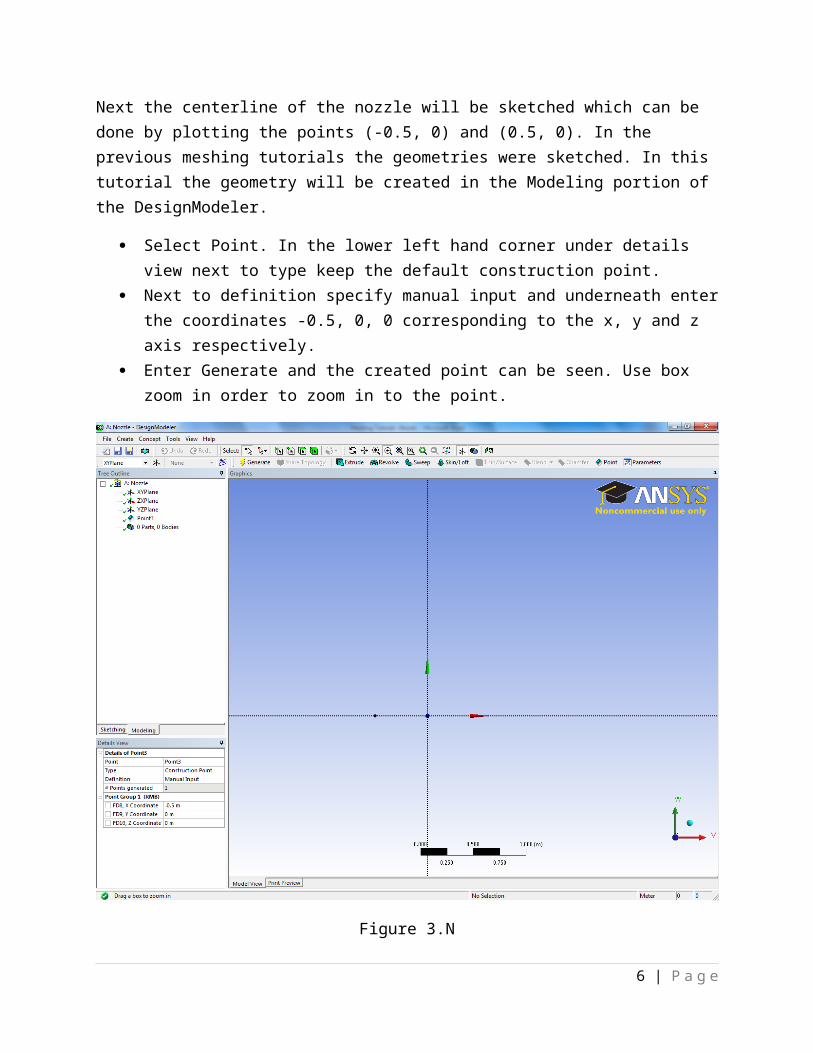
Next the centerline of the nozzle will be sketched which can be done by plotting the points (-0.5, 0) and (0.5, 0). In the previous meshing tutorials the geometries were sketched. In this tutorial the geometry will be created in the Modeling portion of the DesignModeler.

Select Point. In the lower left hand corner under details view next to type keep the default construction point.

Next to definition specify manual input and underneath enter the coordinates -0.5, 0, 0 corresponding to the x, y and z axis respectively.

Enter Generate and the created point can be seen. Use box zoom in order to zoom in to the point.

Figure 3.N

Repeat the same procedure however this time enter the 0.5, 0, 0 coordinates. Enter Generate.

5 | P a g e

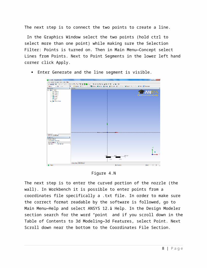
The next step is to connect the two points to create a line.

In the Graphics Window select the two points (hold ctrl to select more than one point) while making sure the Selection Filter: Points is turned on. Then in Main Menu—Concept select Lines from Points. Next to Point Segments in the lower left hand corner click Apply.

Enter Generate and the line segment is visible.

Figure 4.N

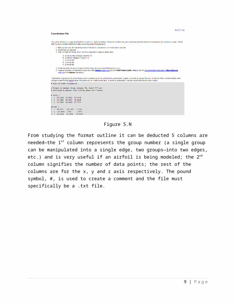
The next step is to enter the curved portion of the nozzle (the wall). In Workbench it is possible to enter points from a coordinates file specifically a .txt file. In order to make sure the correct format readable by the software is followed, go to Main Menu—Help and select ANSYS 12.1 Help. In the Design Modeler section search for the word “point” and if you scroll down in the Table of Contents to 3d Modeling—3d Features, select Point. Next Scroll down near the bottom to the Coordinates File Section.

6 | P a g e

Figure 5.N

From studying the format outline it can be deducted 5 columns are needed—the 1st column represents the group number (a single group can be manipulated into a single edge, two groups—into two edges, etc.) and is very useful if an airfoil is being modeled; the 2nd column signifies the number of data points; the rest of the columns are for the x, y and z axis respectively. The pound symbol, #, is used to create a comment and the file must specifically be a .txt file.

7 | P a g e

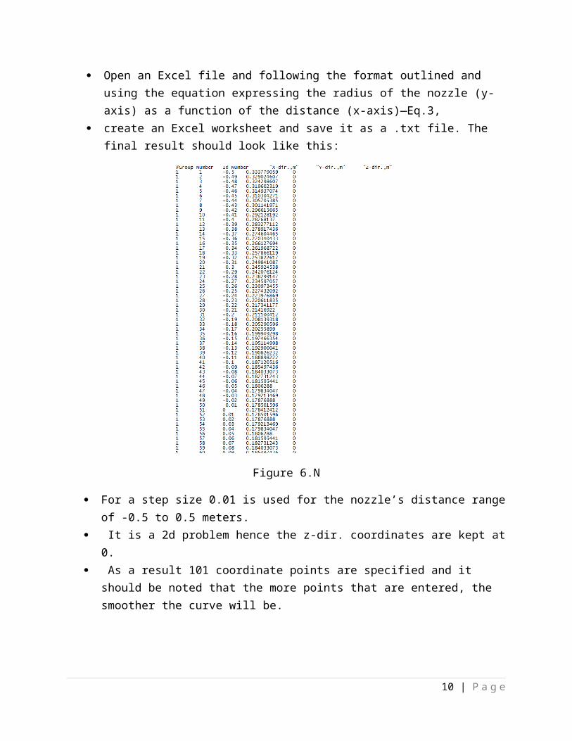
Open an Excel file and following the format outlined and using the equation expressing the radius of the nozzle (y-axis) as a function of the distance (x-axis)—Eq.3,

create an Excel worksheet and save it as a .txt file. The final result should look like this:

Figure 6.N

For a step size 0.01 is used for the nozzle’s distance range of -0.5 to 0.5 meters. It is a 2d problem hence the z-dir. coordinates are kept at 0. As a result 101 coordinate points are specified and it should be noted that the more

points that are entered, the smoother the curve will be.

8 | P a g e

This coordinates file can then be opened in Workbench and fitted to a curve.

In Main Menu—Concept select 3d Curve. In Details View next to Definition specify From Coordinates File. Underneath specify the location of the .txt coordinates file. Click Generate.

Figure 7.N

So far the wall and centerline surfaces have been created—we have 2 edges.

Next the inlet and outlet ones will be modeled.

9 | P a g e

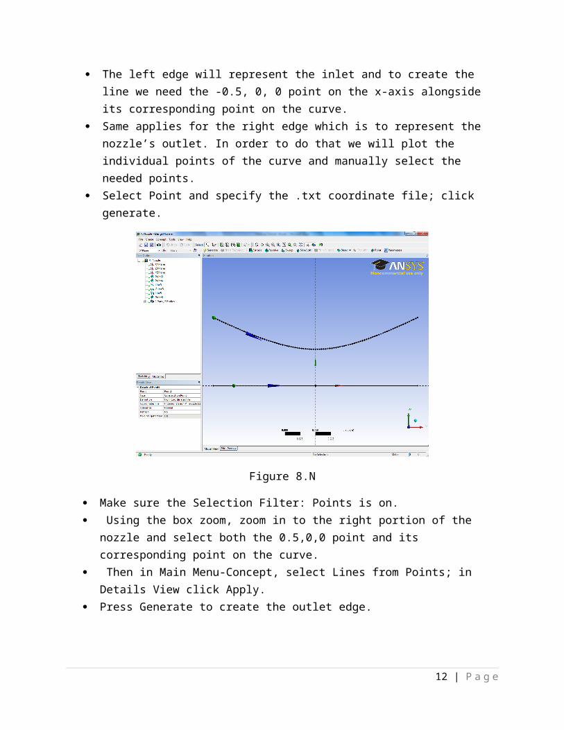
The left edge will represent the inlet and to create the line we need the -0.5, 0, 0 point on the x-axis alongside its corresponding point on the curve.

Same applies for the right edge which is to represent the nozzle’s outlet. In order to do that we will plot the individual points of the curve and manually select the needed points.

Select Point and specify the .txt coordinate file; click generate.

Figure 8.N

Make sure the Selection Filter: Points is on. Using the box zoom, zoom in to the right portion of the nozzle and select both the 0.5,0,0

point and its corresponding point on the curve. Then in Main Menu-Concept, select Lines from Points; in Details View click Apply. Press Generate to create the outlet edge.

10 | P a g e

Figure 9.N

Repeat the procedure for the left portion of the nozzle.

Figure 10.N

The final step before obtaining the geometry for the nozzle is to create the surface from the existing edge.

11 | P a g e

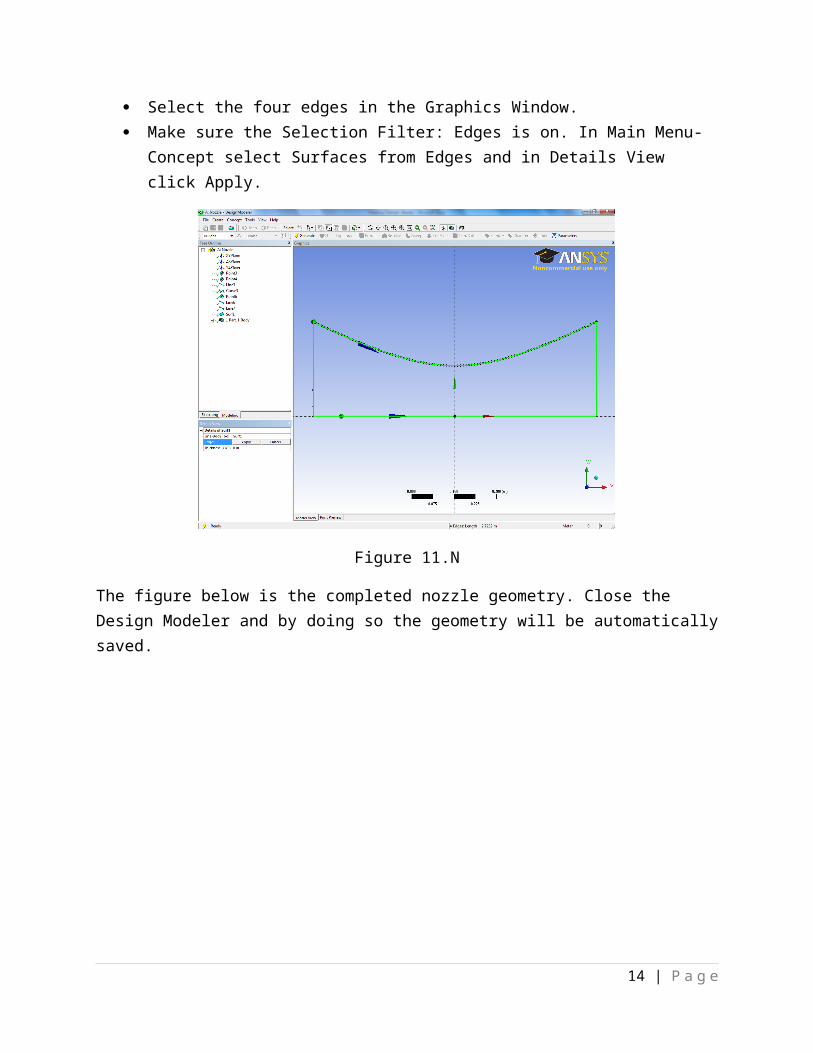
Select the four edges in the Graphics Window. Make sure the Selection Filter: Edges is on. In Main Menu-Concept select Surfaces from

Edges and in Details View click Apply.

Figure 11.N

The figure below is the completed nozzle geometry. Close the Design Modeler and by doing so the geometry will be automatically saved.

12 | P a g e

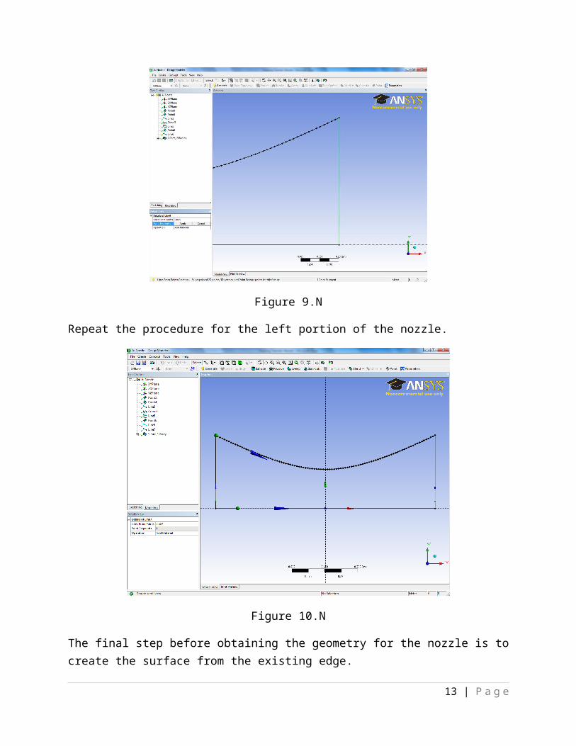
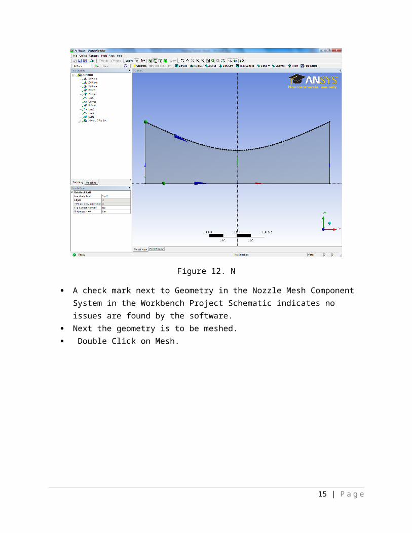
Figure 12. N

A check mark next to Geometry in the Nozzle Mesh Component System in the Workbench Project Schematic indicates no issues are found by the software.

Next the geometry is to be meshed. Double Click on Mesh.

13 | P a g e

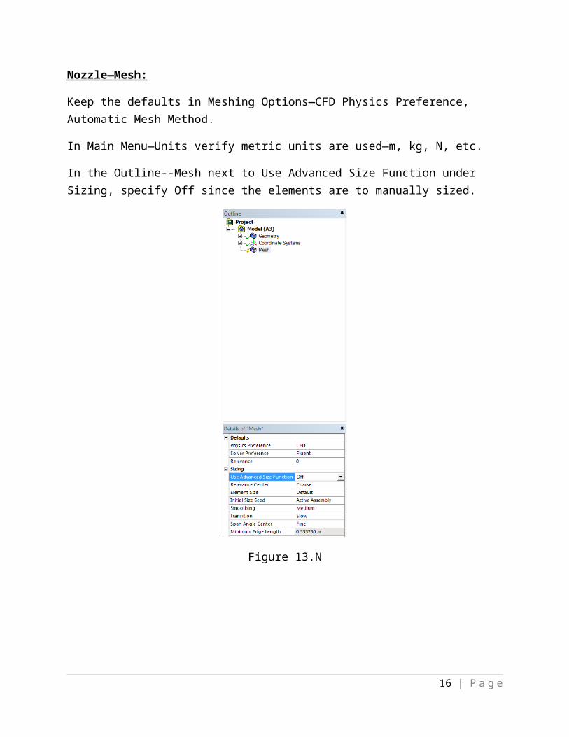
Nozzle—Mesh:

Keep the defaults in Meshing Options—CFD Physics Preference, Automatic Mesh Method.

In Main Menu—Units verify metric units are used—m, kg, N, etc.

In the Outline--Mesh next to Use Advanced Size Function under Sizing, specify Off since the elements are to manually sized.

Figure 13.N

14 | P a g e

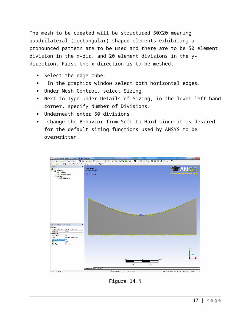
The mesh to be created will be structured 50X20 meaning quadrilateral (rectangular) shaped elements exhibiting a pronounced pattern are to be used and there are to be 50 element division in the x-dir. and 20 element divisions in the y-direction. First the x direction is to be meshed.

Select the edge cube. In the graphics window select both horizontal edges. Under Mesh Control, select Sizing. Next to Type under Details of Sizing, in the lower left hand corner, specify Number of

Divisions. Underneath enter 50 divisions. Change the Behavior from Soft to Hard since it is desired for the default sizing functions

used by ANSYS to be overwritten.

Figure 14.N

15 | P a g e

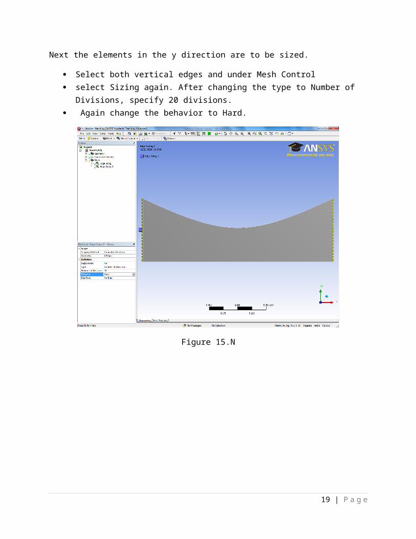
Next the elements in the y direction are to be sized.

Select both vertical edges and under Mesh Control select Sizing again. After changing the type to Number of Divisions, specify 20

divisions. Again change the behavior to Hard.

Figure 15.N

16 | P a g e

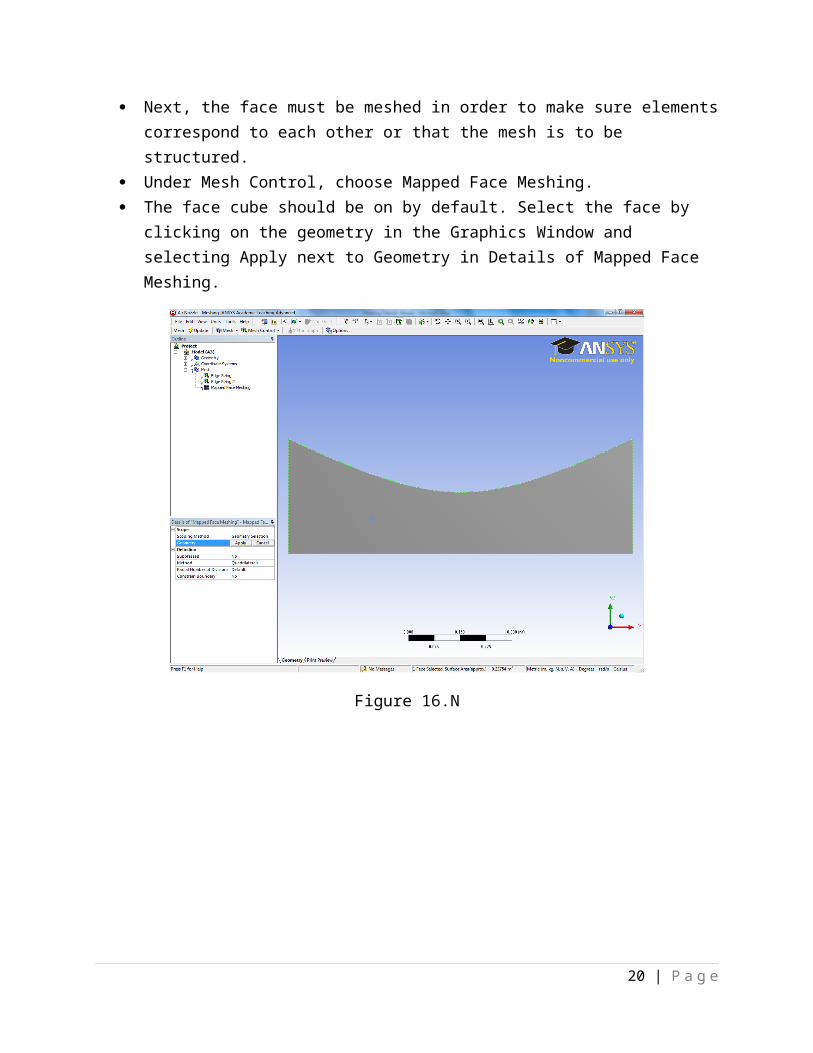
Next, the face must be meshed in order to make sure elements correspond to each other or that the mesh is to be structured.

Under Mesh Control, choose Mapped Face Meshing. The face cube should be on by default. Select the face by clicking on the geometry in the

Graphics Window and selecting Apply next to Geometry in Details of Mapped Face Meshing.

Figure 16.N

17 | P a g e

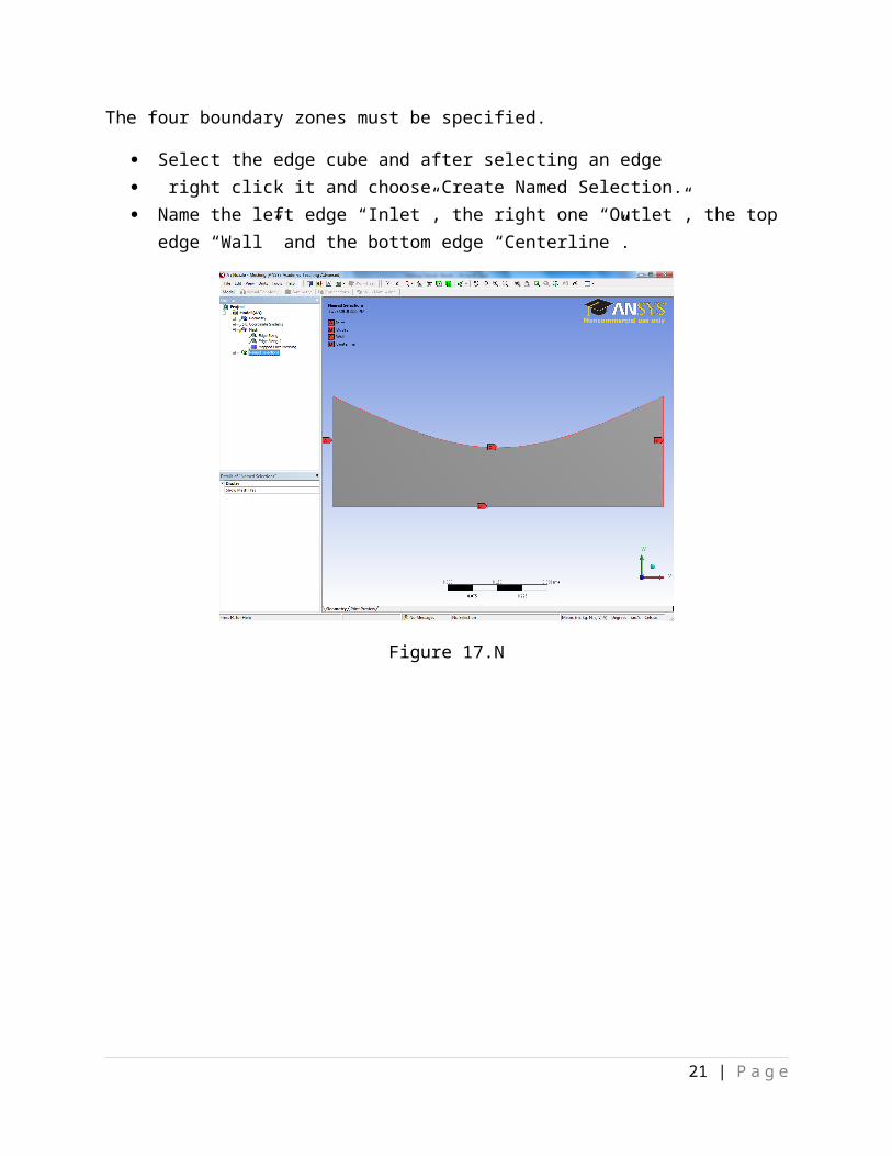
The four boundary zones must be specified.

Select the edge cube and after selecting an edge right click it and choose Create Named Selection. Name the left edge “Inlet”, the right one “Outlet”, the top edge “Wall” and the bottom

edge “Centerline”.

Figure 17.N

18 | P a g e

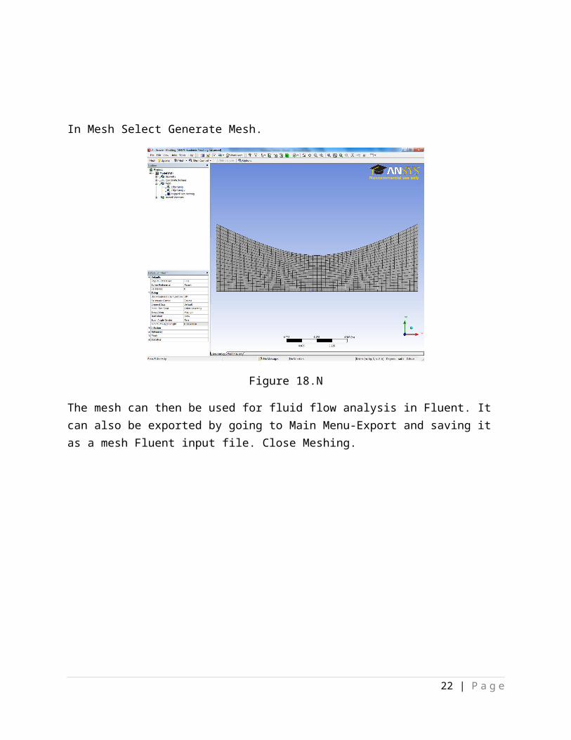
In Mesh Select Generate Mesh.

Figure 18.N

The mesh can then be used for fluid flow analysis in Fluent. It can also be exported by going to Main Menu-Export and saving it as a mesh Fluent input file. Close Meshing.

19 | P a g e

Abstract:

The flexibility of ANSYS Fluent will be demonstrated by analyzing compressible fluid flow past a nozzle by importing the corresponding mesh created in other software such as Gambit. Temperature and pressure effects as well as the Mach number variation will be analyzed and validated against quasi-1D nozzle flow results and particular attention will be paid to the shock developed in the diverging section of the nozzle.

Problem Statement:

Consider a Convergent-Divergent nozzle similar to the one modeled in the Meshing Tutorial—Nozzle:

In a converging-diverging nozzle the flow which enters the nozzle is subsonic (the Mach number, Ma, is less than one). The minimum area is called the throat and is the location when sonic speeds (the Mach number equaling one) are achieved. Referring to equation 1 it can be concluded that for a convergent-divergent nozzle a subsonic flow entering the duct, the flow’s velocity increases upon entering the convergent portion and sonic speed is achieved at the throat. On the other hand if the flow entering the nozzle is supersonic (Ma>1) the velocity decreases in the convergent portion and sonic speeds can be achieved at the throat. Those conditions hold true for steady isentropic flow meaning the properties (such as density, pressure, velocity, etc) are not changing with respect to time and that those properties are functions of the Mach number. Isentropic flow involves constant entropy is adiabatic (no heat transfer) and frictionless (reversible).

dVV

=

−dAA

∗1

(1−Ma2) (1)

The flow to be analyzed is compressible—the Reynolds number and the velocity are large. Since the purpose of a CD nozzle is to accelerate a subsonic velocity to supersonic speeds it makes sense we are dealing with compressible flow. Unlike incompressible flow, the density is not constant anymore. Quasi-one dimensional flow is assumed meaning the flow is restricted to

20 | P a g e

Outlet

Centerline (axis of symmetry)

Inlet

moving in only one coordinate in space (along the x-axis) and the cross-sectional area is allowed to vary in that coordinate. The approach assumes long and slender nozzle geometry and viscous effects are neglect. The last assumption is important since that must be specified in Fluent. The governing equations based on the assumed approach are equations 1 through 5. The flow is also isentropic and the fluid analyzed is assumed to obey the ideal gas law and is necessary in order for the specific heats to be constant.

Consider the following values for the specific flow problem:

Lnozzle=10.0m;Dexit=1.5m;

Lthroat=5.0m;Dthroat=1.0m

T inlet=293.0 K

V inlet=0.24 Ma

Aexit

A throat=1.5;

Ainlet

Athroat=2.5 ;

Poutlet

Pinlet=0.75

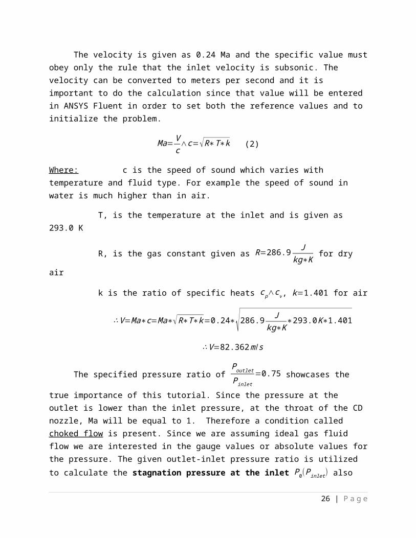
The velocity is given as 0.24 Ma and the specific value must obey only the rule that the inlet velocity is subsonic. The velocity can be converted to meters per second and it is important to do the calculation since that value will be entered in ANSYS Fluent in order to set both the reference values and to initialize the problem.

Ma=Vc∧c=√R∗T∗k (2)

Where: c is the speed of sound which varies with temperature and fluid type. For example the speed of sound in water is much higher than in air.

T, is the temperature at the inlet and is given as 293.0 K

R, is the gas constant given as R=286.9 Jkg∗K for dry air

k is the ratio of specific heats c p∧cv, k=1.401 for air

∴V=Ma∗c=Ma∗√R∗T∗k=0.24∗√286.9 Jkg∗K

∗293.0 K∗1.401

∴V=82.362m/ s

The specified pressure ratio of Poutlet

Pinlet=0.75 showcases the true importance of this tutorial.

Since the pressure at the outlet is lower than the inlet pressure, at the throat of the CD nozzle, Ma

21 | P a g e

will be equal to 1. Therefore a condition called choked flow is present. Since we are assuming ideal gas fluid flow we are interested in the gauge values or absolute values for the pressure. The given outlet-inlet pressure ratio is utilized to calculate the stagnation pressure at the inlet P0(Pinlet ) also referred as the supersonic or initial gauge pressure at the inlet . Equation 2 is used to compute the total gauge pressure at the inlet, P. The equation stems from the assumed Quasi 1D approach and it is important to calculate the pressure since they are to be entered in Fluent. The stagnation pressure is the pressure at a point of zero fluid velocity and kinetic energy has been converted to pressure energy.

PP0

=( 1

1+ k−12

∗Ma2 )k /( k−1 )

(2)

∴ PP0

=( 1

1+ 1.401−12

∗.24 )1.401/( 1.401−1 )

=1.041

However, the pressure of the outlet is 1 atm or 101,325 Pa since the operating pressure is

0 because only the gauge pressures are of interest--pgauge−poperating=0. Recall Poutlet

Pinlet=0.75.

∴P0=poutlet

0.75=101,325

0.75Pa=135,100 Pa

∴P=P0∗1.041=140,639 Pa

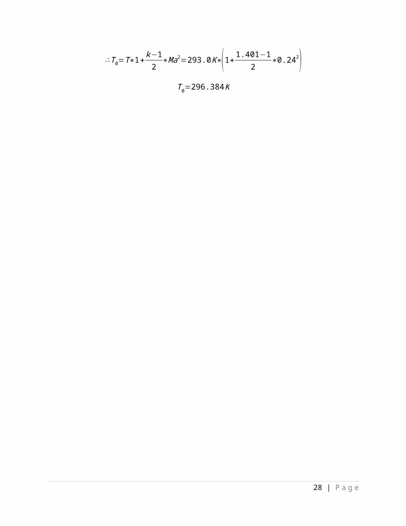
The stagnation temperature must be calculated as well as it will be entered in Fluent. Equation 3is to be used which stems from the assumed Quasi 1D approach. Note T is the inlet temperature and T 0 is the stagnation temperature which is the temperature at a point of zero fluid velocity.

TT0

= 1

1+ k−12

∗Ma2 (3)

∴T 0=T∗1+ k−12

∗Ma2=293.0K∗(1+ 1.401−12

∗0.242)T 0=296.384 K

22 | P a g e

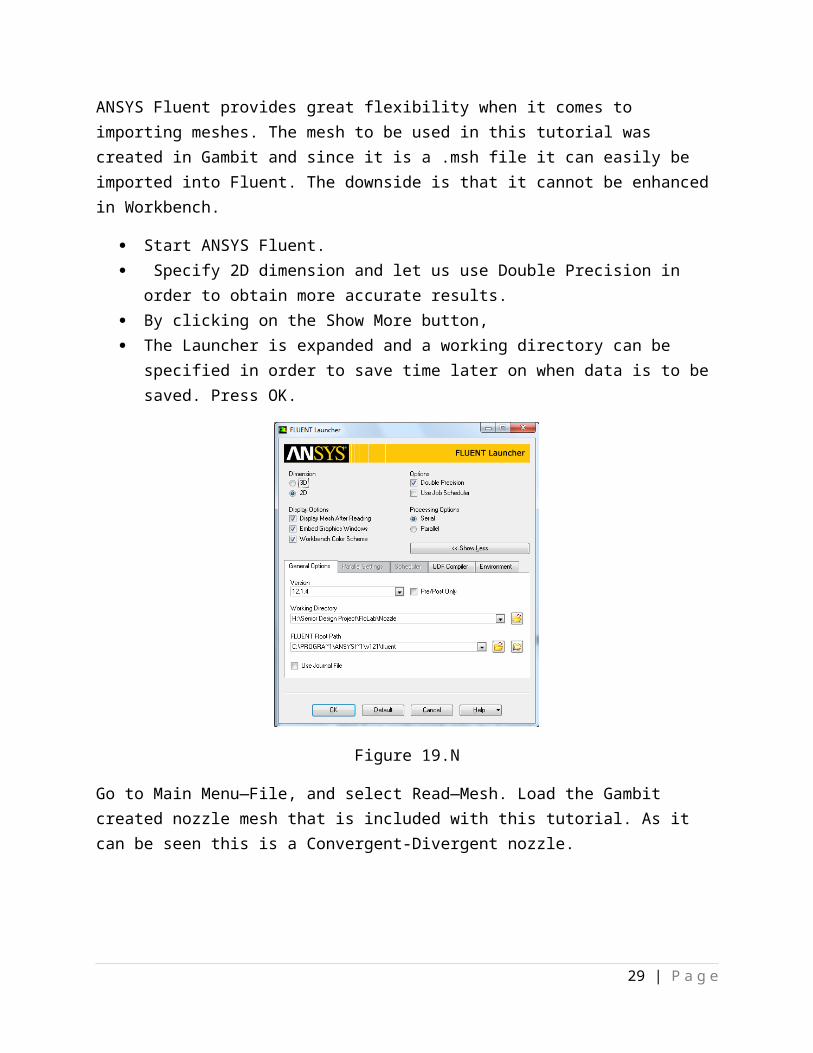
ANSYS Fluent provides great flexibility when it comes to importing meshes. The mesh to be used in this tutorial was created in Gambit and since it is a .msh file it can easily be imported into Fluent. The downside is that it cannot be enhanced in Workbench.

Start ANSYS Fluent. Specify 2D dimension and let us use Double Precision in order to obtain more accurate

results. By clicking on the Show More button, The Launcher is expanded and a working directory can be specified in order to save time

later on when data is to be saved. Press OK.

Figure 19.N

Go to Main Menu—File, and select Read—Mesh. Load the Gambit created nozzle mesh that is included with this tutorial. As it can be seen this is a Convergent-Divergent nozzle.

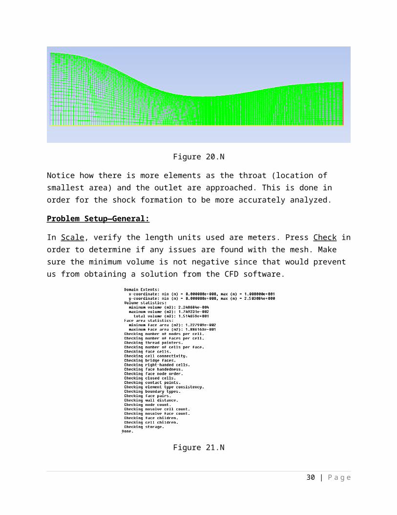
Figure 20.N

23 | P a g e

Notice how there is more elements as the throat (location of smallest area) and the outlet are approached. This is done in order for the shock formation to be more accurately analyzed.

Problem Setup—General:

In Scale, verify the length units used are meters. Press Check in order to determine if any issues are found with the mesh. Make sure the minimum volume is not negative since that would prevent us from obtaining a solution from the CFD software.

Figure 21.N

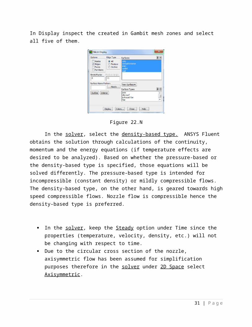
In Display inspect the created in Gambit mesh zones and select all five of them.

Figure 22.N

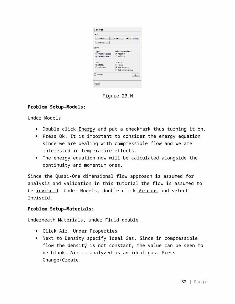
In the solver, select the density-based type. ANSYS Fluent obtains the solution through calculations of the continuity, momentum and the energy equations (if temperature effects are

24 | P a g e

desired to be analyzed). Based on whether the pressure-based or the density-based type is specified, those equations will be solved differently. The pressure-based type is intended for incompressible (constant density) or mildly compressible flows. The density-based type, on the other hand, is geared towards high speed compressible flows. Nozzle flow is compressible hence the density-based type is preferred.

In the solver, keep the Steady option under Time since the properties (temperature, velocity, density, etc.) will not be changing with respect to time.

Due to the circular cross section of the nozzle, axisymmetric flow has been assumed for simplification purposes therefore in the solver under 2D Space select Axisymmetric.

Figure 23.N

Problem Setup—Models:

Under Models

Double click Energy and put a checkmark thus turning it on. Press Ok. It is important to consider the energy equation since we are dealing with

compressible flow and we are interested in temperature effects. The energy equation now will be calculated alongside the continuity and momentum

ones.

Since the Quasi-One dimensional flow approach is assumed for analysis and validation in this tutorial the flow is assumed to be inviscid. Under Models, double click Viscous and select Inviscid.

Problem Setup—Materials:

Underneath Materials, under Fluid double

Click Air. Under Properties

25 | P a g e

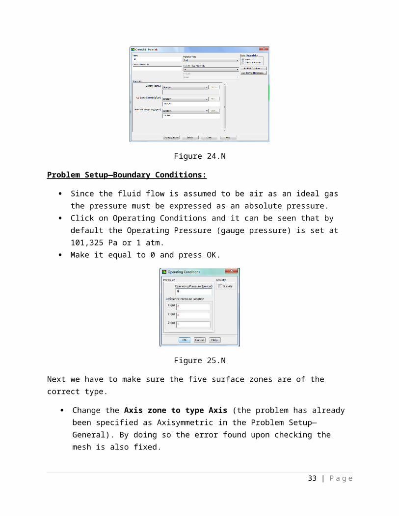
Next to Density specify Ideal Gas. Since in compressible flow the density is not constant, the value can be seen to be blank. Air is analyzed as an ideal gas. Press Change/Create.

Figure 24.N

Problem Setup—Boundary Conditions:

Since the fluid flow is assumed to be air as an ideal gas the pressure must be expressed as an absolute pressure.

Click on Operating Conditions and it can be seen that by default the Operating Pressure (gauge pressure) is set at 101,325 Pa or 1 atm.

Make it equal to 0 and press OK.

Figure 25.N

Next we have to make sure the five surface zones are of the correct type.

Change the Axis zone to type Axis (the problem has already been specified as Axisymmetric in the Problem Setup—General). By doing so the error found upon checking the mesh is also fixed.

Warning: It appears that symmetry zone 4 should actually be an axis

(it has faces with zero area projections).

26 | P a g e

Unless you change the zone type from symmetry to axis,

you may not be able to continue the solution without

encountering floating point errors.

Verify that the wall zone is of type wall, the inlet zone is of type pressure inlet, the outlet zone if of type pressure outlet and the interior zone is of type interior.

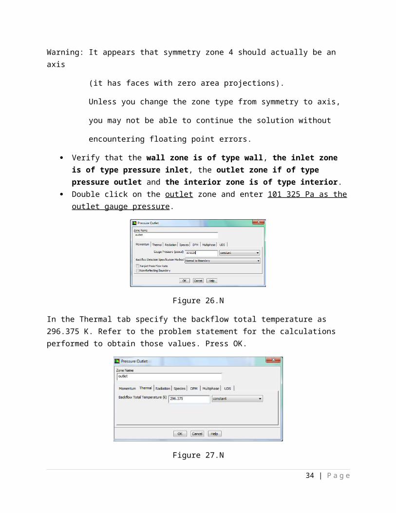
Double click on the outlet zone and enter 101 325 Pa as the outlet gauge pressure.

Figure 26.N

In the Thermal tab specify the backflow total temperature as 296.375 K. Refer to the problem statement for the calculations performed to obtain those values. Press OK.

Figure 27.N

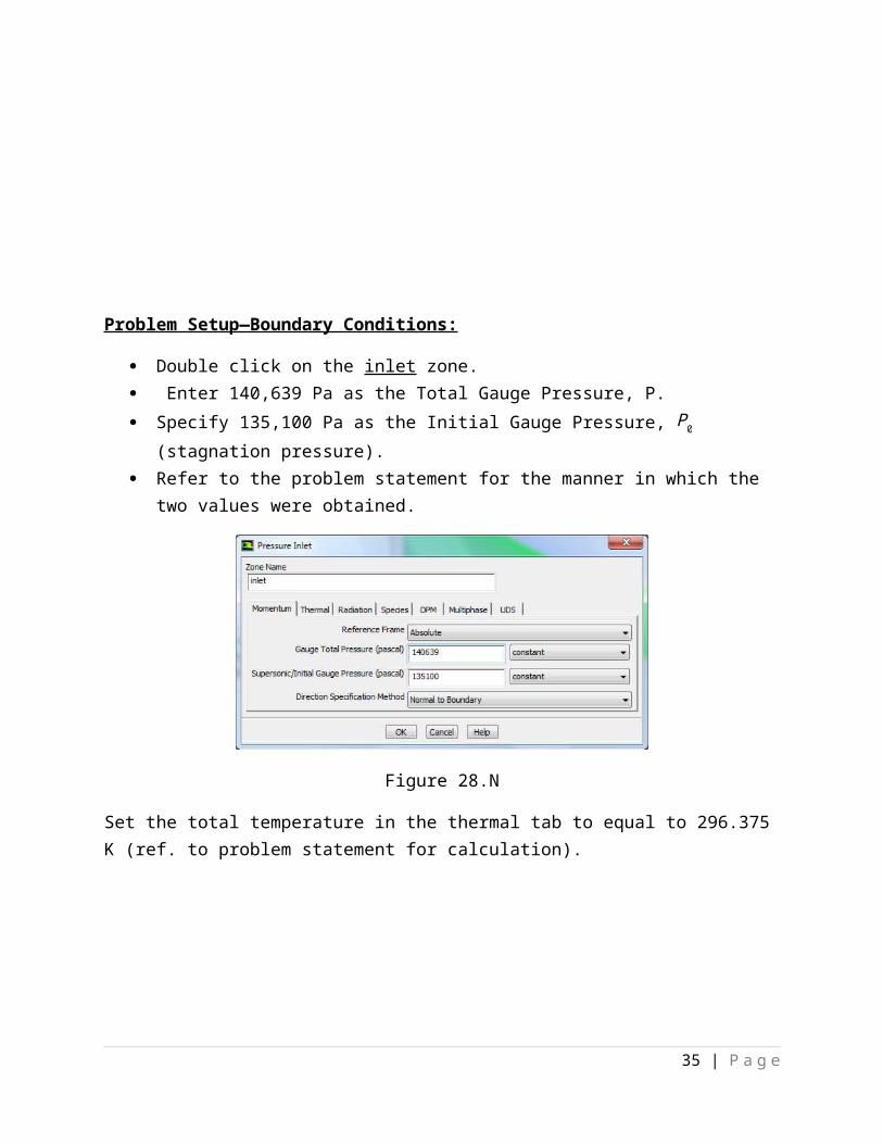
Problem Setup—Boundary Conditions:

27 | P a g e

Double click on the inlet zone. Enter 140,639 Pa as the Total Gauge Pressure, P. Specify 135,100 Pa as the Initial Gauge Pressure, P0 (stagnation pressure). Refer to the problem statement for the manner in which the two values were obtained.

Figure 28.N

Set the total temperature in the thermal tab to equal to 296.375 K (ref. to problem statement for calculation).

Figure 29.N

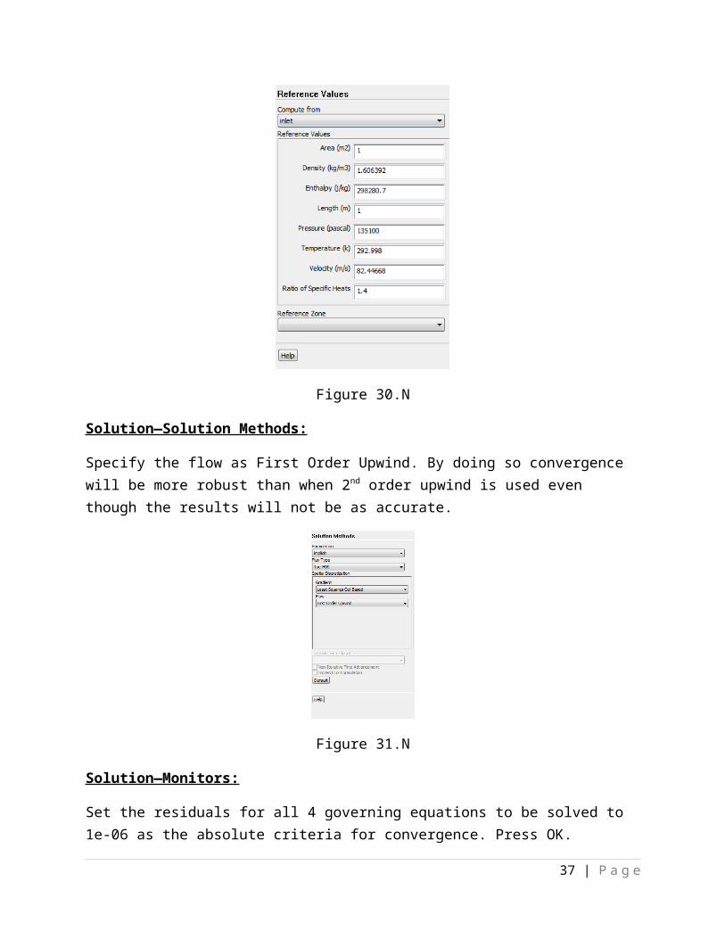
Problem Setup—Reference Values:

28 | P a g e

Set the reference values to be computed from the inlet. Verify the values for temperature and velocity among others make sense. It can be seen there are small variation for the temperature (it was chosen as 293K at the inlet) and the velocity (it was computed as 82.362m /s at the inlet, ref. to Problem Statement Section).

Figure 30.N

Solution—Solution Methods:

Specify the flow as First Order Upwind. By doing so convergence will be more robust than when 2nd order upwind is used even though the results will not be as accurate.

Figure 31.N

Solution—Monitors:

29 | P a g e

Set the residuals for all 4 governing equations to be solved to 1e-06 as the absolute criteria for convergence. Press OK.

Figure 32.N

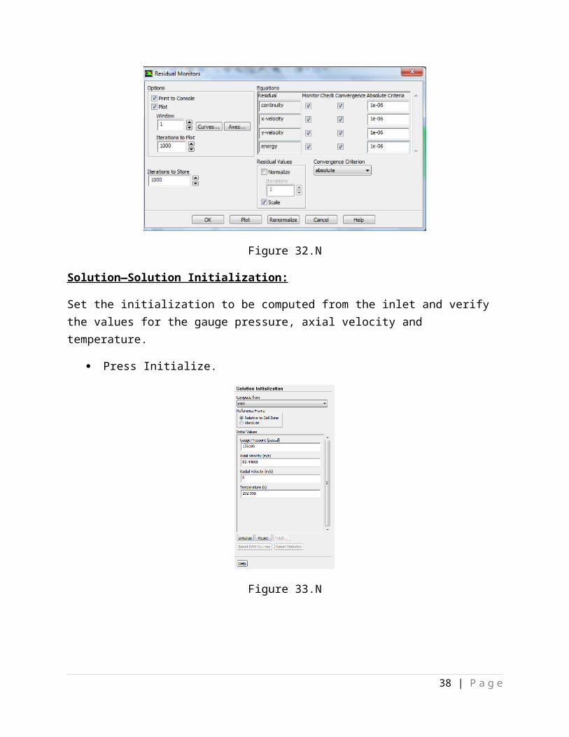
Solution—Solution Initialization:

Set the initialization to be computed from the inlet and verify the values for the gauge pressure, axial velocity and temperature.

Press Initialize.

Figure 33.N

30 | P a g e

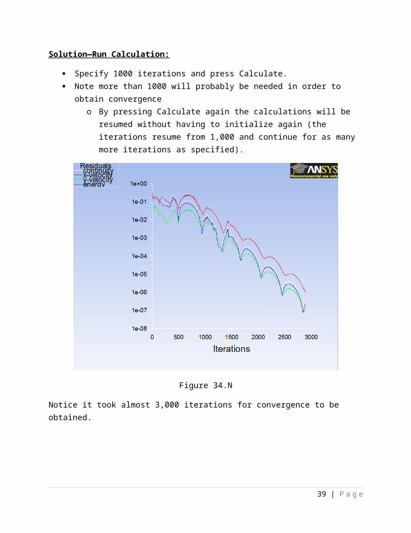
Solution—Run Calculation:

Specify 1000 iterations and press Calculate. Note more than 1000 will probably be needed in order to obtain convergence

o By pressing Calculate again the calculations will be resumed without having to initialize again (the iterations resume from 1,000 and continue for as many more iterations as specified).

Figure 34.N

Notice it took almost 3,000 iterations for convergence to be obtained.

31 | P a g e

Results—Plots:

The temperature, pressure and Mach number are to be plotted as a function of the axial distance both for the wall and axis surfaces.

Temperature XY Plot:

In Plots double click on XY Plot. In Axes, Y axis the type can be specified to float and the precision adjusted to improve

visual representation, remember to click apply (apply makes the requested change only for the specific axis selected).

In Solution XY Plot, make sure the position on x axis is chosen. Under Y axis function, select Temperature and specify Static Temperature. Select both the axis and wall surfaces and press Plot.

Figure 35.N

Figure 36.N

32 | P a g e

To save the XY Plot simply select Write to File under Options in Solution XY Plot and press Write…

The plot can be opened with Excel and further analysis can be performed.

Pressure XY Plot:

For the pressure the only difference is that under Y Axis Function, the Pressure must be chosen.

Save the plot.

Figure 37.N

Figure 38.N

Mach Number XY Plot:

33 | P a g e

The Mach number for the axis and wall surface is next plotted as a function of the axial distance of the nozzle. Under Y axis Function in Solution XY Plot select Velocity and specify Mach Number. Press Plot. Save the Plot.

Figure 39.N

Figure 40.N

34 | P a g e

Velocity Contours:

In Results, in Graphics and Animations,

Double click Contours. Make sure Filled is checked and specify Contours of Velocity, Velocity Magnitude.

Press Display. The significant digits of the colormap can be altered in Graphics and Animations—Colormap.

In Options the colormap can be moved to improved visual representation.

Figure 41.N

Figure 42.N

35 | P a g e

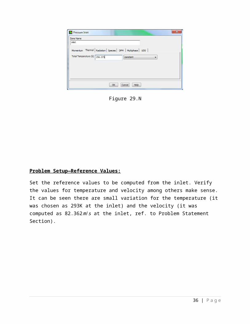
Figure 43.N

The shock inside the nozzle can be clearly seen (circled region). Vast velocity difference is exhibited on each end of the shock.

36 | P a g e

Validation:The Mach number and pressure experimental data along the length of the nozzle is validated against data provided by Prof. Barber. As it can be seen the results strongly agree with the provided data.

Figure 44.N

Figure 45.N

37 | P a g e

Inviscid Results Pe/Pi=0.75

X

0 2 4 6 8 10

Mac

h N

umbe

r

0.0

0.2

0.4

0.6

0.8

1.0

1.2

1.4

1.6

1.8

Maxis Mwall Maxis-visc

0 2 4 6 8 10 120

0.2

0.4

0.6

0.8

1

1.2P_e/P_o at Axis vs Wall

Pe/Po=.75 at AxisPe/Po=.75 at Wall

x, m

P_e/

P_o

Figure 46.N

Figure 47.N

38 | P a g e

Inviscid Pressure Ratio Distribution

X

0 2 4 6 8 10

Pe/P0

0.0

0.2

0.4

0.6

0.8

1.0

Pe/Pi=0.91 Pe/P0=0.75 Pe/P0=0.125

Summary:

After completing the learning module the user has obtained additional valuable knowledge in geometry creation in ANSYS Workbench, specifically importation of coordinates for the creation of curves. That knowledge will be particularly useful for the case discussed in Appendix H when the geometry of a periodic airfoil is considered. Additionally the user has gained further insight in the importance of having sound thermodynamics knowledge as that is necessary for the proper problem setup in FLUENT. Finally additional methods of validation have been provided to the user to ensure the obtained experimental data from FLUENT is reasonable, specifically the data has been validated against provided 1D Quasi Flow data.

39 | P a g e