Comments Welcome

Bank Regulation, Credit Ratings, and Systematic Risk

by

Giuliano Iannotta

Department of Economics and Business Administration Universitá Cattolica

Email: giuliano.iannotta@unicatt.it

and

George Pennacchi

Department of Finance University of Illinois

Email: gpennacc@illinois.edu

First Draft: August 2011 This Draft: November 2012

Abstract

This paper’s model shows that when regulatory capital and deposit insurance are based on credit ratings that reflect expected default losses, a bank’s shareholder value increases when it chooses similarly-rated loans and bonds with greater systematic risk. This moral hazard arises if loan and bond credit spreads incorporate systematic risk premia not accounted for by credit ratings. Consequently, credit rating-based regulations subsidize banks’ systematically risky investments, leading banks to herd into such assets. We confirm the model’s critical assumption by providing evidence that similarly-rated bonds have significantly higher credit spreads when their issuers have higher systematic risk as measured by “debt beta.” We also show that if a bank chooses the higher-yielding bonds within a given Basel Accord credit rating class, its systematic risk rises by an economically significant amount. Our theory explains why banks and capital-regulated insurance companies were motivated to take excessive systematic risks documented in prior research.

Valuable comments were provided by Tobias Berg, Christine Parlour, Andrea Resti, Francesco Saita, João Santos, Andrea Sironi, René Stulz, and participants of the 2011 International Risk Management Conference, the 2011 Bank of Finland Future of Risk Management Conference, the 2012 Financial Risks International Forum, the 2012 Red Rock Conference, the 2012 FDIC Bank Research Conference, the 2012 Banque centrale du Luxembourg Conference, and seminars at Copenhagen Business School, the Federal Reserve Banks of Cleveland and San Francisco, the Federal Reserve Board, HEC Paris, Indiana University, INSEAD, the Korea Deposit Insurance Corporation, Universitá Bocconi, Universitat Pompeu Fabra, and the University of Tennessee. We are very grateful to CAREFIN for providing financial assistance.

 

1. Introduction

Government regulation of banks is pervasive, and its rationale stems from two factors: the inherent fragility

of banks; and the negative externalities from bank failures. Banks provide liquidity by issuing demand

deposits and also act as delegated monitors when making loans to opaque borrowers. This combination of

loan-making and deposit-taking makes banks vulnerable to runs, as they finance relatively illiquid loans with

demandable deposits. Individual bank fragility can, in turn, trigger contagious runs, even on healthy banks,

culminating in system-wide failures with a consequent disruption of credit flows to the rest of the economy.

Government insurance of deposits reduces incentives for bank runs, thereby avoiding contagious bank

failures and their negative spillovers to the economy. However, deposit insurance and other government

assistance, such as central bank lending facilities, can create incentives for banks to take excessive risks. If

unchecked, this moral hazard may lead to large losses by governments when bailing out insolvent banks.

Bank regulation aims to mitigate moral hazard through the setting of capital standards and, in some cases,

deposit insurance premia. However, for regulation to be effective, it must be risk-based in a manner that

neutralizes moral hazard incentives.

The current regulatory framework of risk-based capital and deposit insurance might actually create a

particular form of moral hazard. Specifically, regulation that sets capital and/or insurance premia without

discriminating between systematic and idiosyncratic risks may encourage banks to take excessive systematic

risk; that is, banks will have an incentive to make loans and invest in bonds that are highly likely to suffer

losses simultaneous with an economic downturn. As shown by Kupiec (2004) and Pennacchi (2006), such

moral hazard occurs if regulators measure the risk of a bank’s assets based on their physical (actual)

expected default losses, rather than their risk-neutral expected default losses which reflect the assets’

systematic risks.

For example, under Basel II and III capital regulations, a bank’s required capital is set according to either

external or internal credit ratings. If credit ratings are based on physical – rather than risk-neutral – expected

default losses, credit rating-based regulation will subsidize the bank’s cost of funding investments with

relatively high systematic risk. Why? If, according to asset pricing theory, the credit spread of a loan or bond

contains a systematic risk premium in excess of its expected default losses, then by choosing systematically

1 

 

risky loans and bonds a bank earns high risk premia on its assets without paying the systematic risk cost on

its government-insured liabilities (deposits). The bank can exploit this subsidy, thereby increasing its

shareholders’ value, by simply selecting the highest yielding loans and bonds within each credit rating class.

Such regulation-induced moral hazard can be devastating to banking system stability because banks would

herd into the most systematically risky investments, making simultaneous bank failures particularly sensitive

to economic downturns. Moreover, if regulated intermediaries preferred to fund borrowers with high

systematic risk, the economy’s allocation of capital could be misdirected toward excessively procyclical

projects. Critical empirical questions regarding the validity of this theory are whether credit spreads truly

reflect systematic risk and, if so, whether credit ratings also account for systematic risk to the same degree. If

credit ratings do not incorporate systematic risk to the same extent as credit spreads, then the theory’s

underpinnings would be upheld. These issues are the focus of our paper.

A requirement for credit ratings to reflect systematic risk is that if two similar debt issues have the same

probability of default (PD) and loss given default (LGD), but one is more likely to experience default losses

during a macroeconomic downturn, then that one should receive a lower quality rating. Whether agencies

such as Moody’s and Standard & Poor’s design their credit ratings to discriminate between systematic and

idiosyncratic (nonsystematic) risk is not obvious. Their ratings are assigned “through-the-cycle,” meaning

that a rating neglects transitory components of default risk and, instead, emphasizes default risk during a

business cycle trough. This criterion makes ratings more stable compared to a “point-in-time” assessment of

default risk and could possibly encompass systematic risk since the focus is on default during recessions.

S&P, whose credit ratings are stated to reflect PDs, recently introduced a new stability criterion to its rating

methodology: a lower rating is assigned if “an issuer or security has a high likelihood of experiencing

unusually large adverse changes in credit quality under conditions of moderate stress (for example,

recessions of moderate severity, such as the U.S. recession of 1982 and the U.K. recession in the early 1990s

or appropriate sector-specific stress scenarios)” (Standard & Poor’s 2010). S&P’s revision appears to be the

first time that it explicitly penalizes issuers for systematic, relative to nonsystematic, risk. Moody’s, whose

ratings are viewed to reflect expected default losses (PD×LGD), has not announced a similar revision.

2 

 

Regarding the link between credit spreads and systematic risk, Elton, Gruber, Agrawal, and Mann (2001)

analyzed secondary market corporate bond spreads over the period 1987 to 1996. For bonds of a given credit

rating and maturity, they find that monthly changes in a bond’s credit spread are significantly related to

Fama and French (1993) risk factors. This is suggestive evidence that corporate bond credit spreads may

embed a systematic risk component, even after controlling for their credit rating.1 More recently, Hilscher

and Wilson (2010) find that S&P issuer ratings are related to some measures of systematic default risk and

show that systematic risk also is strongly related to credit spreads. However, they do not test whether spreads

reflect systematic risk beyond that implied by credit ratings.

Our paper begins by employing a standard structural credit risk model to show why banks have an incentive

to invest in highly systematically risky loans and bonds if regulatory capital standards and deposit insurance

premia are based on physical expected default losses, as might be the case when they are tied to credit

ratings. To assess the realism of this model’s assumptions, we carry out three empirical tests. First, we

examine whether credit spreads actually impound systematic risk (as measured by the issuer’s debt beta),

after controlling for credit ratings. Second, we investigate whether credit ratings reflect systematic risk,

either fully, partially, or not at all. Third, we analyze differences between Moody’s and S&P in their

assessment of systematic risk.

Our empirical tests are conducted on an international sample of 3,924 bonds issued during the period from

1999 to 2010. The data comprise credit spreads and issue credit ratings at the time that each bond is

underwritten, along with characteristics of each bond and its issuer. Three main results emerge. First, the

issuer’s debt beta positively affects its bond’s credit spread, even after controlling for the bond’s credit

rating. For example, among bonds of the same rating, those issued by firms with above median debt betas

have much higher spreads compared to those of firms with below-median debt betas. Similarly, if a bank

chooses bonds of a given Basel Accord credit rating class that have above median credit spreads, the

systematic risk of its investments rises by an economically significant amount. In contrast, we find that the

idiosyncratic risk of the issuer’s debt has no impact on credit spreads after accounting for credit ratings. As

                                                            1 They do not explicitly examine whether credit spreads are higher for more systematically risky bonds. While their tests attempt to control for default probabilities, it may be that changes in credit spreads reflect changes in expected default losses that are correlated with systematic risk factors. 

3 

 

such, ratings do not fully incorporate the issuer’s systematic risk, while they do capture idiosyncratic risk.

This result holds even when excluding bonds issued during the financially turbulent period of 2008 to 2010.

Second, for the sample as a whole, credit ratings fail to incorporate any systematic risk. This result, however,

is entirely driven by bonds issued during the financial crisis, when the average level of systematic risk for

debt was abnormally high and only top-rated issuers were able to access bond markets. During the crisis

bonds with high ratings are associated to extremely high systematic risk. When dropping bonds issued during

2008 to 2010, we find that ratings reflect some information about the issuer’s systematic risk. Nonetheless,

the fact that bond investors require a systematic risk premium, after controlling for credit ratings, suggests

that raters do not fully account for systematic risk (at least not as much as do investors). Third, while

Moody’s and S&P do not differ significantly in their assessments of systematic risk, the likelihood of a split

rating (disagreement between raters over the same issue) decreases with the issuer’s beta. This finding may

be explained by high-beta issuers’ default risks being strongly correlated with systematic factors, which

raters are more likely to agree upon compared to firm-specific factors.

By showing that credit spreads incorporate a systematic risk premium not accounted for by credit ratings, our

paper’s empirical work is a test of our model’s assumptions rather than a test of the model’s implications.

Ideally, one would like to analyze banks’ actual holdings of loans and bonds to see if they choose the most

systematically risky ones among a given rating class. Unfortunately, such detailed data on banks’ portfolio

holdings is not publicly available, making a direct test of the theory difficult. However, at the end of the

paper we discuss informal evidence that many banks were attracted to highly-rated but systematically-risky

investments. We also review empirical evidence on the portfolio choices of insurance companies which, like

banks, are subject to credit rating-based capital regulation.

The paper proceeds as follows. Section 2 presents the model and discusses why current bank regulation

creates incentives to take excessive systematic risk. Section 3 describes our data sources and presents

summary statistics. Section 4 addresses the question of whether credit spreads reflect an issuer’s systematic

risk. In Section 5 we look at the impact of the issuer’s systematic risk on its credit ratings, while in Section 6

we test for any difference between Moody’s and S&P’s assessment of systematic risk. Section 7 discusses

empirical evidence from other studies that relate to our model’s predictions, while Section 8 concludes.

4 

 

2. A model of a regulated bank

This section’s model predicts that the current structure of bank regulation creates incentives for banks to take

excessive systematic risk. Our subsequent empirical work tests the basic assumptions of the model and

thereby assesses the credibility of this implication. The model is similar to the binomial models in Kupiec

(2004) and Pennacchi (2006), but uses the continuous-time framework of Merton (1974, 1977) and Galai and

Masulis (1976) which is better suited to guide our empirical analysis.

2.1. Model assumptions

A bank issues government-insured deposits and is subject to risk-based capital standards. At the initial date

0, the bank has insured deposits of D0 upon which it pays the competitive, default-free interest rate of r. The

bank’s shareholders also contribute equity capital equal to K0. Therefore, the bank initially has D0 + K0

available to invest in a portfolio of default-risky bonds and loans whose date 0 value is denoted A0 = D0 + K0.

The bank’s portfolio is allocated to the debt of firms in m different industries, where each industry is exposed

to a different source of risk. All firms have a capital structure that satisfies the assumptions in Merton (1974).

Appendix A shows that if the portfolio’s proportions invested in the m different industries are kept constant

over time, then the rate of return on the bank’s portfolio can be written as

,1

mtA i ii

t

dA dt dzA

dt dz

μ σ

μ σ

== +

= +

∑ (1)

where σA,i is the volatility of returns from the bank’s loans and bonds of firms in industry i, dzi is the

Brownian motion process specific to firm asset returns in industry i, dzidzj = ρijdt, 2, ,1

m m

A j A i ijj iσ σ σ ρ

==∑ ∑ ,

and 1,1

m

A i iidz dzσ σ

=≡ ∑ . In addition, if the Capital Asset Pricing Model (CAPM) holds, Appendix A shows

that the expected rate of return on the bank’s asset portfolio satisfies the CAPM relationship

1

mM i ii

rμ ϕ ω=

= + β∑ (2)

5 

 

where ϕM is the excess expected return on the market portfolio of all assets, ωi is the bank’s proportion of

total assets held in bonds and loans of firms in industry i, and βi is the average debt beta of firms in industry

i. Appendix A details how debt betas are calculated based on Galai and Masulis (1976).

A government regulator sets a risk-based capital standard and a deposit insurance premium for the bank. The

bank’s insurance premium is determined at date 0 but payable at a future date T, which also is the time that

the bank is audited by the regulator. Let p be the (continuously-compounded) annual insurance premium rate

per deposit. The premium to be paid at date T equals DT(epT-1), so that the total amount of deposits plus

insurance premium payable at date T is DTepT = D0e(r+p)T .2 Similar to Merton (1977), if at the audit date AT <

D0e(r+p)T, the bank is declared to have failed and is closed or merged with another institution. The government

regulator/deposit insurer incurs any loss required to pay off insured deposits.

2.2. Fair capital standards and insurance premia

These assumptions imply that there are three claimants on the bank’s assets: depositors, bank shareholders,

and the government regulator/insurer. Because insured depositors obtain a default-free claim that pays the

competitive default-free rate r, the date 0 value of their claim on the bank’s assets is always worth D0.

Denote the date 0 values of claims on the bank’s assets by shareholders and by the government regulator as

E0 and G0, respectively. Then

0 0 0 0 0A D K D E G= + = + + 0

                                                           

(3)

or K0 = E0 + G0. When capital standards and/or deposit insurance premiums are set fairly, G0 = 0, so that E0 =

K0 =A0 – D0; that is, the value of the shareholders’ claim on the bank equals the funds that they contribute. If

G0 < 0, so that E0 > K0, then a government subsidy transfers value to the bank’s shareholders. In general, the

value of the regulator’s claim can be computed as

 2 This form makes the insurance premium analogous to a credit spread on deposits if deposits were uninsured. In the absence of deposit insurance and regulation, uninsured depositors would set the credit spread, p, to make the date 0 fair value of their default-risky deposits equal D0, the amount they contribute initially. 

6 

 

[ ] ( )( )( )

( ) ( )

0 0 0 0

0

E E max ,0

E min 1 ,

1 E max ,0

rT Q rT Q pTT T T T

rT Q pTT T T

pT rT Q pTT T

G A D E

e A D e A D e

e D e A D

D e e D e A

− −

−

−

= − −

⎡ ⎤= − − −⎣ ⎦⎡ ⎤= − −⎣ ⎦

⎡= − − −⎣⎤⎦ (4)

where EQ[·] denotes the “risk-neutral” or Q-measure expectations operator. It computes expectations based

on the risk-neutral asset return process

Qt

t

dA rdt dzA

σ= + (5)

Equation (4) shows that the claim of the government regulator/insurer equals the value of its premium

income, D0(epT – 1), minus the value of a put option written on the bank’s assets, e-rTEQ[max(DTepT-AT ,0)]. If

G0 = 0, so that there is no subsidy, equation (4) implies that the present value of the insurance premium

revenue must equal the value of losses from the bank’s failure:

( ) ( )( ) ( ) (

( )

0

0 2 0 0

0 0 0

1 E max , 0

, ,

pT rT Q pTT T

pT

pT

D e e D e A

D e N d K D N d

Put K D D e T

− ⎡ ⎤− = −⎣ ⎦= − − + −

≡ +

)1 (6)

where ( )( ) ( )21 0 0 0ln / /pTd K D D e Tσ σ⎡ T= + +⎣

⎤⎦ and 2 1d d Tσ= − . Equation (6) is a relationship

between the bank’s required capital, K0, and its deposit insurance rate, p, that leads to no government subsidy

to the bank. It equates the present value of premiums to the value of a put option written on assets currently

worth A0 = K0 + D0, having an exercise price with present value D0epT, and a time until maturity of T.

2.3. Insurance premia and capital standards in practice

Importantly, the current structures of deposit insurance and capital requirements differ from equation (6)

because they are based either purely on physical, rather than risk-neutral, expected default losses or on

external credit ratings or internal ratings that imperfectly reflect risk-neutral expected default losses. We now

7 

 

explain why this is so for FDIC insurance premia and capital requirements based on the Basel II and III

“Standardized Approach” and “Internal Ratings-Based Approach.”3

FDIC Insurance: The FDIC attempts to calibrate risk-based insurance premia to cover a bank’s expected loss

claims due to failure, where expected losses are calculated using physical probabilities, not risk-neutral

ones.4 There is no adjustment to consider a bank’s systematic, as opposed to idiosyncratic, risk of failure. As

discussed in Pennacchi (1999), the overall level of insurance premia typically are set to target a level of

FDIC Deposit Insurance Fund (DIF) reserves,5 and incorporating an appropriate systematic risk component

in insurance premia would lead to DIF reserves that, on average, exceed their target. Consequently, the

objective of targeting DIF reserves conflicts with the setting of fair deposit insurance premia.

Basel Standardized Approach: The clearest link between capital standards and credit ratings occurs under the

Standardized Approach. It sets credit risk weights, which determine capital requirements, as a function of

external bond and loan credit ratings. For corporate claims, credit risk weights are 20%, 50%, 100%, and

150% for bonds or loans rated AAA to AA-, A+ to A-, BBB+ to BB-, and below BB-, respectively. Thus, for

a given rating category, there is no scope for distinguishing between high and low systematic risk bonds and

loans. Equivalently, the capital charge for a given rating category reflects only a single level of systematic

risk. Indeed, Gordy (2003) derives capital standard risk weights based on a single risk factor model (global

CAPM) that assumes a fixed level of systematic risk for all claims of a given credit rating category.

Basel Internal Ratings Based Approach: Under Basel’s “Internal Ratings Based (IRB) Approach,” which is

followed by the largest globally-active banks, credit risk capital charges also are based on the single risk

                                                            3 While our discussion focuses on Basel capital requirements for “credit” risks, there is evidence that banks may rely on external credit ratings even when computing Basel capital requirements for “market” risks. In 2008 the Swiss Federal Banking Commission required that UBS report the key causes of its severe losses during the recent financial crisis. UBS’s report to shareholders (UBS, 2008) is uniquely insightful as to the risk management practices of large banks. It states that external credit ratings were used to determine “the relevant product-type time series to be used in calculating VaR” (p. 20). Moreover, an over-reliance on credit ratings, which appears to be common across the industry, was found to be a primary cause of UBS’s losses as “a comprehensive analysis of the portfolios may have indicated that the positions would necessarily perform consistent with their ratings” (p. 39). 4 For example, see Federal Register 76 (38) February 25, 2011 which details amendments to the Federal Deposit Insurance Act that were made to comply with the Dodd-Frank Act. An underlying principle for setting premiums (assessments) is stated on page 10700: “Under the FDI (Federal Deposit Insurance) Act, the FDIC’s Board of Directors must establish a risk-based assessment system so that a depository institution’s deposit insurance assessment is calculated based on the probability that the DIF (Deposit Insurance Fund) will incur a loss with respect to the institution.” The FDIC’s statistical failure probability models, on which its premium schedule is based, use physical, rather than risk-neutral, probabilities of bank failures. 5 The current DIF reserve target is between 1.35% and 1.50% of insured deposits. 

8 

 

factor portfolio model analyzed in Gordy (2003). Inputs into the capital charge formula are the bank’s own

estimates of its bonds’ and loans’ physical probabilities of default (PD) and losses given default (LGD).6 The

Basel formula then converts these physical inputs into their hypothetical risk-neutral counterparts using an

assumed beta or market correlation of each asset class.7 It is important to emphasize that this assumed beta

(correlation) is not chosen by the bank but is set by Basel IRB rules.8

Thus, under the Basel Standardized Approach, the implicit beta reflected in a capital charge for a given

external credit rating may differ from the true beta of a bank’s loan or bond of that same credit rating.

Likewise, under the Basel IRB Approach, the assigned beta for an asset class may differ from the true beta of

a bank’s loan or bond belonging to that asset class. Consequently under both approaches, while a bank’s true

expected rate of return on assets is given by 1

mM i ii

rμ ϕ ω=

= + β∑ as in equation (2), the Basel rules would

assign an implicit beta or systematic risk assessment implying1

mB M i

r i iBμ ϕ ω=

= + ∑ where Bi is the average

Basel estimated beta for loans or bonds of industry i based on their assigned asset classes. Thus, if the Basel

rules do not appropriately discriminate between loans’ and bonds’ systematic risks for a given asset class, it

may be that Bi ≠βi and μB ≠ μ.

Therefore, because actual deposit insurance premia and regulatory capital standards implicitly assume

uniform systematic risk across broad asset and credit rating classes, they may inaccurately reflect risk-neutral

expected losses. Taking account of the difference between true and estimated betas, the actual standard that

is the counterpart to the fair standard in equation (6) is:

                                                            6 Under the “Foundation” IRB approach, regulators fix LGD for corporate claims. For example, it is 45% for all senior, unsecured bonds and loans. Under the “Advanced” IRB approach, guidelines recommend that banks estimate a bond or loan’s “downturn” LGD, which reflects losses that are expected to occur if default happens during an economic downturn. Use of downturn LGDs may in principle differentiate between high and low systematic risk claims, but since PDs are not conditioned on a downturn, the VaR capital requirement is unlikely to fully incorporate systematic risk.  7 Since

,, /i Mi i A i Mρ σω β σ= , where ρi,M is the correlation between the market risk factor and the asset class i’s return, an

assumption regarding the correlation ρi,M essentially is an assumption regarding the asset class’s beta. 8 IRB rules require sufficient initial capital, K0, such that there is no more than a 0.1% physical probability of losses exceeding this initial capital over a one-year horizon. The VaR capital requirement formula assumes correlations with the market risk factor (betas) that differ across classes of credit risky claims. In principle, these correlations could distinguish between claims with high and low systematic risk claims. However, correlation values are the same for broad classes of bonds and loans. For corporate bonds and loans, the correlation value varies between 8% and 24%, but the variation is a function only of the borrowing firm’s annual sales (greater for firms with more than €50 million in sales) and the bank’s estimated physical PD, where correlation is higher for lower PDs. See BCBS (2005). Fitch Ratings (2008) finds no empirical support for the IRB rule’s inverse relationship between PDs and portfolio correlation (systematic risk). As will be reported in our empirical work, neither do we find an inverse relationship between a firm’s systematic risk (debt beta) and its probability of default (as reflected in its credit rating).  

9 

 

( ) ( ) ( ) ( ) ( )( ) ( )( )

0 0 2 0 0

0 0 0

1

, ,

B

B

TpT pT B B

T pT

D e D e N d K D e N d

Put K D e D e T

μ μ

μ μ

−

−

− = − − + −

= +

1 (7)

where ( ) ( )( ) ( )21 0 0 0ln / /B TB pTd K D e D e Tμ μ σ σ−⎡ T= + +⎣

⎤⎦ and 2 1

B Bd d Tσ= − . Note that in equation (7)

if μB = μ, then the relationship between insurance premia and required capital is exactly that of the fair case

in equation (6). However, when μB ≠ μ, the Basel rules incorrectly convert physical expected losses to risk-

neutral expected losses, and the fair insurance premia and capital requirement relationship reflects the

deviation, μ - μB. The actual premia and required capital relationship when this error occurs leads to the same

Black-Scholes put option pricing formula as (6) except that the underlying asset value ( )0 0K D+ is

everywhere replaced with the underlying asset value ( ) ( )0 0

B TK D e μ μ−+ . Because put options are decreasing

functions of the value of the assets on which they are written, when μ > μB the value of the put option in

equation (7) is less than that in equation (6):

( ) ( )( ) ( )0 0 0 0 0 0 if , , , , BB

T pT pTPut K D e D e T Put K D D e Tμ μ μ μ− >+ < + (8)

An implication of inequality (8) is that when a regulator uses equation (7) to set insurance rates, p, and

capital standards, K0, they are lower than what is required to satisfy the no-subsidy relationship in equation

(6). Consequently, from equation (4), G0 < 0. In turn, equation (3) implies E0 = K0 – G0 > K0, so that the

subsidy provided by the regulator accrues to the bank’s shareholders. Specifically, since shareholders’ equity

has a payoff analogous to a call option, its value is

( )( )( ) ( ) (

0 0

0 0 1 0 2

E max ,0

r p TrT QT

pT

E e A D e

K D N d D e N d

+−

)

⎡ ⎤= −⎣ ⎦= + −

(9)

and since and( ) ( )0 0 0 1/ 1E K K N d∂ − ∂ = − < 0 ( ) ( )0 0 0 2/ 0pTE K p pD e N d∂ − ∂ = − < , when capital

standards and/or insurance premia are lower than those satisfying the fair equation (6), a subsidy flows to

bank shareholders. The greater is (μ - μB), the greater is the difference between the put option in equation (6)

versus that in equation (7) and the greater is the government subsidy transferred to shareholders.

10 

 

Indeed, one now sees from equation (2) that a bank can increase the subsidy accruing to its shareholders by

raising the relative systematic risk of its bond and loan portfolio, (1

mB M i i ii )Bμ μ ϕ ω β

=− = −∑ . It can do so

by selecting greater portfolio weights, ωi, in industries where the average debt beta of firms is high relative to

the assumed Basel debt beta. Also, within an industry, the bank could select those bonds and loans of firms

with relatively high debt betas, thereby raising the average relative debt beta in that industry, (βi - Bi). Such

portfolio decisions need not change the overall volatility of the bank’s asset portfolio, σ, but even if they do,

the relative subsidy for any given level of portfolio volatility, σ, still increases.

Our model suggests that banks will intentionally take excessive systematic risk to increase the government

subsidy that accrues to their shareholders. But it is possible that more naïve banks will do so unintentionally.

Why? Note that controlling for physical expected default losses, bonds or loans with greater systematic risk

will have larger credit spreads or yields to maturity. This is because if the debt beta of the ith bond or loan is

βi, its expected rate of return is r + ϕMβi. All else equal (including expected default losses), higher systematic

risk in the form of a higher debt beta raises the expected rate of return of the bond or loan, which must lower

its price relative to its promised payment, thereby raising its yield and credit spread.

Thus, if a naïve bank subject to credit rating-based capital charges simply chooses bonds and loans that have

the highest credit spread or yield for a given credit rating, it will automatically pick relatively high beta

bonds and loans. By simply selecting top-yielding bonds and loans within a given rating class, the bank may

inadvertently be loading up on systematic risk and, in turn, receiving a greater government subsidy.

The model implies that banks will herd into systematically risky loans and investments, thereby creating a

systemically risky banking system. Other models predict that banks may choose common exposures, though

not necessarily by investing assets with relatively high systematic risk. Penati and Protopapadakis (1988)

develop a model where banks are bailed out by the government if a sufficiently high proportion of them

become insolvent at the same time. The bailout takes the form of de facto government insurance of the

insolvent banks’ uninsured liabilities. As a result, banks have an incentive to over-invest in similar loans.9

Acharya and Yorulmazer (2007) provide a rationale for why governments would grant such bailouts, even

                                                            9 They give as an example banks’ large amounts of lending to less developed countries (LDCs) during the late 1970s and early 1980s. In equilibrium, the incentive to herd in these LDC loans pushed interest rates below competitive levels.  

11 

 

though they are time-inconsistent policies: allowing many banks to simultaneously fail leads to insufficient

surviving banks that could efficiently deploy the failed banks’ assets. Many governments’ reactions to the

recent financial crisis appear to confirm these papers’ predictions. Several banks were bailed out by their

national governments through provisions that range from the guarantee of uninsured debt to equity capital

injections. Consistent with their models, one way that banks could achieve common exposures would be to

lend to borrowers with high systematic risk, since they tend to default together during economic downturns.

However, our argument is different from these papers’ “too many to fail” rationale for government bailouts

that create moral hazard by banks. We claim that capital charges or deposit insurance premia based on credit

ratings can lead an individual bank to take more systematic risk, even if other banks do not and even if the

bank is not bailed out but is allowed to fail.10 An individual bank chooses to do so because credit rating-

based regulation, which determines the bank’s cost of funding, fails to discriminate between defaults in good

versus bad times. However, credits spreads on loans and bonds, which determine the bank’s revenue, does

reflect the systematic risk of defaults.

The next sections consider whether the main assumptions of our model have empirical validity. We examine

the relationships between credit spreads, credit ratings, and systematic risk based on an international sample

of bonds which we now describe.

3. Data

We obtained data on new bond issues over the 1999 to 2010 period from DCM Analytics, which reports

information on each bond issuer (nationality, industry, etc.) and each bond issue’s characteristics (credit

spread, credit rating of the issue, years to maturity, face value, maturity date, currency, etc.). Our sample is

restricted to fixed-coupon bonds that are non-convertible, non-perpetual, and non-callable. The initial sample

consists of 9,691 bonds that have complete information about the issue. We focus on investment grade

issues, which reduce the sample to 7,413 bonds. Because this data contains issue ratings and new issue

spreads, it is ideal for testing whether or not credit ratings and spreads incorporate similar information. Since

agencies assign the issue rating at the time of issuance, this primary market data avoids problems of stale

                                                            10 Consequently, even if legislative reforms, such as the Dodd-Frank Act, prevented government bailouts, our theory predicts that banks would continue to herd into systematically risky investments. 

12 

 

ratings: issue ratings should impound all information available to the rating agency at the time of issuance,

the same time when the bond’s initial credit spread is set by investors.11

We then use Bloomberg to match each bond ISIN code with the issuer’s corresponding stock ISIN code. Our

final sample consists of 3,924 bonds issued by 620 listed firms, mostly from North America, Europe, and

Japan. For each bond, we collected from Bloomberg the issuer’s stock returns for the 52 weeks prior to the

bond’s issuance date along with the contemporaneous weekly returns of the MSCI World Index. As a

robustness check, we repeated our analysis by using the issuer’s domestic stock index rather than the MSCI

World, with no relevant change in our main findings. We employ a standard market model to estimate the

issuer’s stock (equity) beta. While the equity beta reflects shareholders’ exposure to systematic risk, the

theoretically appropriate measure of the systematic risk faced by the firm’s bondholders is the firm’s debt

beta. Moreover, bond credit spreads should reflect debt betas. As detailed in Appendix A, we follow Galai

and Masulis (1976) to derive the firm’s debt beta from its equity beta, assuming a debt maturity of 10 years.

As a robustness check, we also computed debt betas with maturities of 1 and 5 years, and the main results of

the paper are confirmed. We also compute the equity residual volatility as a measure of idiosyncratic risk.

From this variable we derived debt residual volatility. As discussed in Appendix A, our calculations of a

bond issuer’s debt beta and residual volatility do not use information on the new bond issue itself, but instead

rely on the issuer’s stock market and balance sheet information just prior to the bond issue.

Table 1 provides mean values of some relevant issue and issuer characteristics by rating class (Panel A) and

by year (Panel B). For summary statistics we use letter ratings (AAA/Aaa, AA/Aa, A/A, etc.) as opposed to

notch-level ratings (AAA/Aaa, AA+/Aa1, AA/Aa2, AA-/Aa3, etc.) to have a greater number of observations

per rating class. A bond’s credit spread is defined as the difference between the bond’s yield at issuance and

the yield on a Treasury security of the same maturity and currency of denomination. As expected, the

average credit spread at issuance increases monotonically as ratings worsen. There are only 132 issues with

top ratings of AAA/Aaa, with an average credit spread of about 80 basis points (bp). BBB/Bbb rated bonds,

the worst class among investment grade issues, have an average credit spread of almost twice as much at 149

bp. Top-rated bonds also have a much shorter maturity of 4.8 years compared to the 8.1 year maturity of all                                                             11 Other studies have sometime used issuer ratings and secondary market bond spreads. Relative to the information content of secondary market spreads, issuer ratings may become “stale” because they are adjusted only infrequently and may reflect new information only with a lag.

13 

 

other rating classes. Should ratings reflect systematic risk, one might expect worse-rated bonds to have a

higher beta. In fact, top rated bonds tend to have greater betas and residual volatility (both debt and equity)

compared to issuers of bonds with worse ratings. The reason that AAA/Aaa bonds have remarkably larger

betas is that the majority were issued by financial institutions during the years 2008 to 2009 (99 out of 132)

at the height of the financial crisis when systematic risk was abnormally high. Figures 1 and 2 plot the

average of issuers’ equity and debt betas for the entire 1999 to 2010 sample and also for the sample

excluding issues that took place during the financial crisis (year 2008 and beyond). Issuers of top-rated bonds

have much lower betas when dropping observations in 2008 and after. Moreover, taking the financial crisis

out of the picture, debt betas are clearly increasing as ratings worsen. Equity betas of the issuer have a less

clear pattern, as even excluding the financial crisis, they appear relatively stable across rating classes.

Turning to the time evolution of the main sample variables, Panel B of Table 1 shows that the mean credit

spread decreases from over 100 bp during the 1999 to 2001 period to a minimum of 46 bp by 2005; then it

keeps increasing until reaching its maximum of 215 bp during the financial crisis year of 2009. The mean

spread during the 1999 to 2005 period is 82.8 bp as opposed to 146.9 bp from 2006 to 2010. Interestingly,

the mean rating shows the opposite trend. The mean rating is 6.2 (about A/A2) during 1999 to 2005, while it

is about one notch better (A+/A1) from 2006 through 2010. This pattern presumably reflects a “flight to

quality” during the financial crisis when only high-quality issuers were able to tap debt markets. Figures 3

and 4 show the time series evolution of equity and debt betas of the issuing firms. Equity betas average 1.17

in year 1999 and tend to decrease to a minimum of 0.69 in 2006. Starting in 2007 it constantly increases to a

maximum of 1.13 in 2010. Average debt betas follow a similar pattern, although they are relatively more

variable. From a level of 0.15 in 1999, debt betas steadily drop to 0.01 in year 2005 and 2006. They then

increase dramatically to 0.22 in 2009. This substantial rise reflects, in part, that a firm’s debt beta increases

as the market value of the firm’s net worth declines.12

The next section examines whether credit ratings are a good proxy for the risk embedded in bond credit

spreads, or whether an issuer’s systematic risk is an additional determinant of spreads. We begin with some

informal evidence followed by more rigorous regression analysis.

                                                            12 See equation (A4) of Appendix A. As a firm’s asset value declines relative to its promised debt payments, its debt’s risk becomes closer to that of its assets since a default, after which debtholders own the assets, becomes more likely. 

14 

 

4. Do credit spreads reflect issuers’ systematic risk beyond that implied by credit ratings?

4.1. A preliminary look

A simple way to determine whether credit spreads embed systematic risk beyond any systematic risk

reflected in credit ratings is to compare the mean spreads of bonds with different systematic risk that have

the same rating. Let us first define bonds with high (low) systematic risk those having issuer betas higher

than (lower than or equal to) the sample median. We exclude bonds rated AAA/Aaa for which we have a

limited number of observations (132). Table 2 reports the mean spreads for bonds with high and low

systematic risk for the three different rating classes: AA, A, and BBB. We also control for whether the

bond’s maturity was 10 years or less versus greater than 10 years. A rationale for doing so might be that

issuers’ systematic risk influences their choice of bond maturity, and it may be maturity, rather than

systematic risk, that is reflected in spreads.

In Panel A of Table 2, bonds are classified according to their issuer’s equity beta. Within the same rating

class, bonds of issuers with high systematic risk pay a much larger spread. For example, the average AA

bond with maturity less than 10 years and low systematic risk pays about 67 bp. Equally-rated bonds with

high systematic risk pay an average of 107 bp. The 40 bp difference is statistically significant at the 1%

level. Similar significant differences emerge in the other rating classes, irrespective of maturity. The only

exception is the BBB class with maturities exceeding 10 years: however, there are only 107 bonds with such

features, of which 36 (71) have high (low) systematic risk. When excluding bonds issued in the years 2008

and beyond, we obtain similar results, although the magnitude of the systematic risk premium is smaller. The

spread difference between bonds with high versus low equity betas (across all rating classes) is about 36 bp

for the whole sample, while it drops 15.2 bp when excluding the financial crisis period.

Panel B of Table 2 sorts bonds of a given rating class by their issuers’ debt betas, which theory implies is the

appropriate measure of the bonds’ systematic risk (rather than the issuers’ equity betas). There we see that

the spread difference between high versus low systematic risk bonds appears even larger. The systematic risk

premium (across all rating classes) is about 56 bp. As before, the spread difference between bonds with high

and low debt betas drops when excluding bonds issued in the 2008 to 2010 period, from 56.5 bp to 19.6 bp.

15 

 

Table 3 is similar to Table 2 Panel B except that it separates bonds by currency denomination (rather than

maturity) and debt beta quartiles (rather than above and below the median). The first (fourth) quartile of a

given currency and rating class is the 25% of bonds of that currency and rating whose issuers had the lowest

(highest) debt betas. Table 3 also attempts to more finely control for differences in ratings at the notch level

within a class. It adjusts spreads for each reported quartile based on differences in the quartile’s average

rating at the notch level.13 The results in Table 3 are striking. For each major currency and rating class, there

is a general tendency for spreads to rise as the issuers’ debt betas (systematic risks) increase. In all 12 cases,

spreads for the issuers in the highest quartile of systematic risk are significantly larger than spreads for

issuers in the lowest quartile of systematic risk.

4.2. A bond picking exercise

Our model predicts that credit rating-based regulation allows banks to increase their shareholder value by

selecting bonds and loans with excessive systematic risks. They do so by selecting investments with the

highest credit spreads for a given credit rating, which raises systematic risk that is ignored by regulations.

Indeed, as discussed earlier, a particular bank may not intentionally choose to load on high systematic risk

investments, but it may do so unwittingly by investing in the top-yielding bonds and loans within a given

rating class that determines its required capital. Such a bank may naively believe that it is exploiting a market

inefficiency when picking the highest yielding bond or loan of a given credit rating.

To show how this mechanism can work, we categorize all bonds in our sample by year of issuance, maturity

(lower versus higher than 10 years), currency (Euro, US Dollar, and Yen), and credit rating. To be consistent

with the Standardized Approach of Basel II, we use ratings at the letter level (as opposed to the notch level)

and merge AAA-rated bonds with AA-rated bonds.14 For each category that has at least five issues, we rank

bonds based on their credit spreads and compute the average debt beta of bonds with credit spreads above the

median of the category (high-spread bonds). We then compare this value with the average debt beta of all the                                                             13 For each currency and rating class, we regress spreads on their notch-level ratings, obtaining a slope coefficient, say α, indicating the unconditional rise in spreads for a unit change in notch-level rating. To the raw average spread for each quartile we add ( class quartileR Rα × − ) , where classR is the average rating for the entire class and quartileR is the average rating for the particular quartile. In the absence of any systematic effects of debt beta, this adjustment would equalize spreads for differences in average ratings across quartiles. However, the results in Table 3 are little affected by this adjustment because differences in average rating across quartiles were small. 14 Recall that Basel II’s Standardized Approach assigns risk weights of 20%, 50%, 100%, and 150% to corporate claims rated AAA to AA-, A+ to A-, BBB+ to BB-, and below BB-, respectively. 

16 

 

bonds in the category. Table 4 reports the result of this exercise. Panels A and B show betas for bonds with

maturities of 10 years and less versus greater than 10 years, respectively. In most of the categories, the

average issuer beta of high-spread bonds is greater than the average beta of all of the bonds in the category.

For example, suppose that in the year 2003 a bank had to choose among Euro-denominated, A-rated bonds

with maturities of 10 years or less. Within this category, the average beta of bonds with credit spreads above

the median is 0.192 compared to an average beta of 0.133 for all bonds in this category. Similarly, for U.S.

dollar-denominated, BBB-rated bonds issued in 2009 with a maturity exceeding ten years, those bonds with

above median credit spreads had an average issuer debt beta of 0.329, while the average issuer debt beta for

all bonds in the category was 0.239.

To test whether these results are statistically significant, for each category in Table 4 we compute the ratio of

the average issuer beta of high-spread bonds to the average issuer beta of all the bonds in the category. If

choosing a high-spread bond had no relationship with the bond issuer’s debt beta, the natural log of this ratio

should have an unconditional value of zero. In Table 5 we report the results of a t-test, conducted for all the

categories across both calendar years and currency, as well as for categories with the same currency. We can

reject the hypothesis that mean log ratios are equal to zero both when looking at all currencies together and

for all but one category with the same currency.15 The results in Table 5 show that if a bank simply selected

bonds with credit spreads above the median for any given Basel II credit rating category, it would be

investing in bonds having debt betas (systematic risk) approximately 20% above average. This appears to be

an economically significant increase in systematic risk relative to random bond selection.

Of course, the above median selection criterion assumed in Tables 4 and 5 is arbitrary. Moral hazard could

be worse if banks selected bonds having spreads in the highest quartile or decile. For example, the debt betas

of issuers in the top spread quartile of US dollar-denominated A and BBB bonds and Euro-denominated A

and BBB bonds are above their respective rating class averages by 35%, 55%, 59%, and 70%, respectively.

For these four classes of bonds, suppose that Basel capital standards were calibrated using the average debt

betas of all bonds in each rating class, but banks selected bonds in the top quartile of spreads. Then

calculations using equations (6) and (7) with typical-bank parameter values would show that fair capital for

                                                            15 The only exception is Japanese yen-denominated bonds with maturities exceeding 10 years. While this category’s log ratio is positive, it may lack significance due to relatively few observations. 

17 

 

banks that held US-A, US-BBB, Euro-A, and Euro-BBB bonds would need to be 6.5%, 10.0%, 11.4%, and

16.5% greater than the total required capital set by the Basel standards.16

So far, the evidence suggests that bond investors require a credit spread premium for bonds with higher

systematic risk within the same rating class. In other words, credit ratings fail to capture all of the systematic

risk reflected in credit spreads. However, to control for other issue and issuer characteristics that might

influence credit spreads, we next move to more formal multivariate statistical tests. We start by investigating

whether credit spreads impound the issuers’ systematic risk when controlling for credit ratings as well as

other issue and issuer characteristics.

4.3. Regression analysis

To test whether bond investors price the systematic risk of an issuer’s debt, we run a regression of credit

spreads on the bond issuer’s debt beta, controlling for credit ratings and other issue and issuer characteristics.

Specifically, consider the following specification:

( )( ), ,, , ln ,i t i tSpread f Rating Debt Beta Debt Residual Volatility Controls ε= + (10)

where:

Spread The bond’s credit spread, equal to the difference between the bond’s yield at issuance

and that of a Treasury security of the same currency and maturity.

Rating A series of nine dummy variables indicating the issue rating at the notch level.

AAA/Aaa is the excluded rating variable.

Debt Beta The issuer’s debt beta estimated over the 52 weeks preceding the issue.

Debt Res. Vol. The issuer’s debt residual volatility estimated over the 52 weeks preceding the issue.

Controls Issue’s and issuer’s characteristics that might affect the credit spread, including the

issue face value, maturity, issuer’s country, year, and currency fixed effects. A detailed

                                                            16 These calculations assume σ = 4%, T = 1, and a fixed deposit insurance premium of p = 10 bp. Given these parameters, equation (6) implies fair capital equal to 6.23% of assets (K0 = 0.0623×A0). Assuming a market risk premium of ϕm = 8%, equation (7) is then used to calculate capital under the Basel standards where μ-μB = (β-B)ϕm, where β is the average debt beta for bonds in the rating class’ top quartile of spreads and B is the average debt beta for all bonds in the class. Because these calculations are based on the Black-Scholes model, which is well-known to understate the likelihood of extreme losses, they are meant only for illustrative purposes.

18 

 

description of control variables is reported in the Appendix B.

We estimate OLS regressions with robust standard errors clustered at both the year and the issuer level.

Table 6 reports results. In Column 1 we include only ratings and control variables. Rating dummies are all

strongly significant and increase monotonically as the bond’s rating worsens. Despite the recent criticism

about the accuracy and timeliness of rating agencies, our empirical evidence indicates that credit ratings are

an important determinant of bond yield spreads. For example, a AA+/Aa1 rated bond pays about 74 bp more

than AAA/Aaa bond (the excluded category), while the credit spread of a BBB-/Bbb3 rated bonds is about

211 bp larger than a top-rated bond. In Column 2 we include the debt beta, whose coefficient is positive and

strongly significant. Column 3 shows that debt beta continues to be strongly significant after the issuer’s debt

idiosyncratic volatility is added to the regression, whereas debt idiosyncratic volatility is insignificant.17 The

debt beta coefficient of 105.4 implies that a one standard deviation increase in an issuer’s debt beta of 0.136

raises the bond’s credit spread by 14.3 bp. Since the regression’s credit rating dummies imply that a

worsening of one notch raises the credit spread by 15.7 bp, on average, this one-standard deviation higher

debt beta impacts the spread only slightly less than would a notch downgrade.

Earlier we noted that bonds issued during the financial crisis have better issue ratings, notwithstanding a

remarkably higher systematic risk. The association between good ratings and high systematic risk observed

from 2008 to 2010 might bias our results, leading to an over-estimate the systematic risk premium required

by investors. We thus run regressions excluding bonds issued in the years 2008 and beyond. Results are

reported in Column 4 of Table 6. Two main findings emerge.

First, the premiums for lower quality ratings relative to a AAA/Aaa rating are much smaller for all rating

notch classes, reflecting the ease of tapping debt markets in the pre-crisis era. For example, while in the

whole sample the average BBB-/Bbb3 bond pays about 208 bp more than a AAA/Aaa rated bond, excluding

the financial crisis the figure drops to 76 bp, roughly the same as a AA+/Aa1 in the whole sample. In

addition, when excluding the financial crisis a AA+/Aa1 bond does not have a significantly higher credit

                                                            17 The idiosyncratic volatility of the issuer’s debt is insignificant presumably because it is fully captured by credit ratings. Indeed, in unreported results, we find that the coefficient of debt residual volatility becomes significant when rating dummies are excluded from the regression.

19 

 

spread than a top-rated bond. In particular, credit spreads for the whole AA/Aa rating class (including bonds

with ratings equal to AA+/Aa1, AA/Aa2, AA-/Aa3) are not statistically different from that of a AAA/Aaa

bond if we exclude 2008 to 2010. Therefore, it seems that in the pre-crisis era bond investors relied on credit

ratings mostly to discriminate between just the best and the worst of investment-grade bonds. This result is

particularly relevant in light of banks’ capital regulation. Under Basel II and III, claims rated from AAA to

AA- have the same risk weight (20% for claims on corporates). Based on our evidence, this approach proves

correct in “normal” times: in contrast, under stress conditions, investors clearly discriminate between a AAA

bond and each notch-level rating within the AA class.

Second, although strongly significant, the coefficient of the debt beta variable is smaller compared to the

whole sample regression (67.8 versus 108.8). It is therefore plausible that a structural increase in the

systematic risk premium required by investors occurred during the financial crisis. In Column 5 we test the

effect of the interaction between a dummy for the financial crisis years (2008-10) and the issuer’s debt beta.

As expected, the interaction term is positive and strongly significant, suggesting that investors required a

much higher systematic risk premium after 2008.18

For robustness, we estimated issuer debt betas and residual volatilities by assuming a maturity of 5 years

(instead of 10 years) and re-ran all the regressions. The main findings are all confirmed.

4.4. Controlling for liquidity

Spreads between corporate bonds and Treasuries may reflect not only credit risk but also illiquidity. In the

regressions reported in Table 6, we controlled for a number of issue characteristics, including the issue size,

which should proxy for a bond’s secondary market liquidity. However, suppose for some reason investors

were reluctant to trade bonds with high systematic risk, so that bonds of issuers with high debt betas were

viewed as less liquid. If so, such bonds should be priced less at issuance and have higher spreads. Thus,

because credit ratings do not account for bond liquidity, what our previous regression analysis of credit

spreads presumes to be a systematic risk premium might actually be a liquidity risk premium. To address this

concern, we conduct an additional test, controlling for a bond’s observed liquidity in the secondary market.

                                                            18 Berg (2010) analyzes the term structure of credit default swap (CDS) spreads and also finds a rise in the short-term systematic risk premium during the financial crisis. 

20 

 

A commonly used measure of liquidity is the relative bid-ask spread (Chordia et al. 2005; Goyenco and

Ukhov, 2009), which is computed as follows:

( )12

100Ask BidBid Ask SpreadAsk Bid

−− =

+× (11)

where Ask and Bid are the quoted ask and bid prices for a given day.

For each bond in our sample, we searched Bloomberg for its bid and ask quotes for each day over the first 60

trading days following its issuance. From these quotes we computed the average relative bid-ask spread,

deleting any daily observations with a spread equal to zero or negative. We were able to find and compute

the average relative bid-ask spread, Avg Bid-Ask Spread, for a subsample of 2,395 bonds (out of the total

sample of 3,924 bonds).

For this 2,395 bond subsample, regressions similar to those reported in Table 6 were run except that the

variable Avg Bid-Ask Spread was also included as a control. By using this control for expected illiquidity, we

implicitly assume that investors purchasing a bond on the primary market can foresee with reasonable

accuracy the spread between bid and ask quotes that will prevail on the secondary market. The results of

these regressions are reported in Table 7. As expected, larger secondary market bid-ask spreads are

associated with a higher bond “credit” spread in the primary market, consistent with a liquidity premium. But

most importantly, our previous main findings are all confirmed. Credit spreads still reflect debt systematic

risk after controlling for credit ratings, even a bit more strongly than before when the bid-ask spread was

excluded. For example, the debt beta coefficient of 139.5 in the full regression in Column 3 implies that a

one-standard deviation increase in debt beta raises the spread by 19.4 bp (=139.5×0.139). Since the

regression’s rating dummies imply that a one notch worse rating raises the spread by 13.7 bp, on average,

this one-standard deviation higher debt beta is equivalent to a worsening of 1.4 notches. Finally, Columns 4

and 5 show that debt beta continues to be significant even when separating out the financial crisis years.

To sum up, our results suggest that credit spreads required by bond investors incorporate systematic risk

beyond that reflected in credit ratings. In contrast, once one controls for credit ratings, credit spreads do not

appear to reflect the issuer’s idiosyncratic risk. Put another way, credit ratings seem to be based on physical

21 

 

expected default losses, while investors value bonds based on risk-neutral expected default losses. However,

we cannot reject the hypothesis that ratings at least partially impound information about the issuer’s

systematic risk. Indeed, it is possible that investors assign a different weight to systematic risk than raters do.

In the next section we check whether issue ratings reflect issuers’ systematic risk by running regressions of

ratings on the issuers’ debt betas, volatilities, and other issue and issuer controls.

5. Do credit ratings reflect issuers’ systematic risk?

From statements by credit rating agencies, issue ratings would seem to reflect a bond’s physical probability

of default, as would be the case if raters considered only the issuer’s total default risk and not whether

default tends to occur during economic expansions versus economic recessions. In contrast, if raters

differentiated between idiosyncratic and systematic default risk, then ratings might reflect risk-neutral

probabilities of default if defaults in bad economic times were weighted relatively greater.

Both Moody’s and S&P claim that normal fluctuations in economic activity and the consequent effects on

the credit quality of an issuer or issue are impounded into their credit ratings. In other words, ratings are

assigned “through the cycle.” Whether this approach includes an assessment of systematic risk is unclear. On

the one hand, an evaluation of the possible adverse consequences of an economic slowdown on a credit

rating would arguably imply an analysis of the bond’s systematic risk. On the other hand, if raters place

probabilities on the likely occurrence of different economic scenarios equal to their physical (actual), rather

than risk-neutral, probabilities, then their calculations of expected default or expected default losses will not

equal risk-neutral expected default or default losses. For example, an issuer with high systematic risk might

be considered extremely vulnerable to a recession, but if the probability of a recession is not weighted

greater than its physical probability, ratings will not reflect risk-neutral expected default losses.

Recently, S&P announced new ratings criteria (Standard & Poor’s, 2008, 2010) that suggests it may be

switching from using physical default probabilities to something akin to risk-neutral ones. The President of

S&P, Deven Sharma, summarized this change with the statement “Under S&P’s new criteria,…we may feel

that two securities have similar default risk, but if we believe one is more prone to a sharp downgrade in

periods of economic stress, it will be rated lower initially.” Such a rating methodology might have the

potential to place greater weight on default losses during an economic downturn.

22 

 

To investigate the information content of credit ratings, we first compute the average issue rating (Avg

Rating), equal to the average of Moody’s and S&P’s issue ratings converted into a numerical scale

(AAA/Aaa = 1, AA+/Aa1 = 2, …, BBB-/Bbb3 = 10). We then run the following OLS regression, with robust

standard errors clustered at both the year’s and the issuer’s level:

( )( ), , , ln ,i t i tRating f Debt Beta Debt Residual Volatility Controls ε= + (12)

Results are reported in Table 8. In Column 1 we exclude the residual volatility of the issuer’s debt and only

analyze the effect of systematic risk. The coefficient of the debt beta variable enters positive and significant.

Recall that a higher value of Rating indicates a worse issue rating. Notably, however, when including the

issuer’s idiosyncratic risk, the debt beta becomes insignificant (Column 2). Results are very similar when

replacing the idiosyncratic (residual) volatility of the issuer’s debt with the total volatility of the issuer’s debt

(Column 3).

As noted earlier, the financial crisis produced two relevant effects on the bond market, which are clearly

detectable in our sample: i) primarily issuers of good quality could access the market, thus resulting in better

average issue ratings; and ii) the average systematic risk of issuers increased dramatically. As a result, during

the crisis bonds with good ratings are associated with very high issue betas, therefore possibly biasing our

results towards the finding that ratings do not account for systematic risk. Indeed, by focusing on the sub-

sample of bonds issued before 2008, a different picture emerges. Ratings do reflect systematic risk (Column

4), even when controlling for the residual or total volatility of the issuer’s debt (Columns 5 and 6).19

However, the effect seems small. For example, based on the debt beta coefficient of 1.682 in Column 5, a

one standard deviation increase debt beta would worsen the rating by only 0.18 of a notch (=1.682×0.1079).

In contrast, from our results in the previous section a one-standard deviation increase in debt beta raised the

spread by an amount equivalent to about one full notch or more. The results imply that raters may partially

account for systematic risk, but not as much as bond investors.

                                                            19 Results (unreported) are unchanged when using debt and residual volatility estimated assuming a 5-year maturity (instead of 10 years).

23 

 

It is nonetheless possible that the granularity of the discrete rating scale does not accurately reflect a

continuous variable such as the systematic risk of the issuer’s debt. However, the same discrete rating scale

seems to properly capture the level of the debt’s idiosyncratic and total risk, which also are continuous.

Whether it is a matter of granularity of rating scales or rather an under-weight of systematic risk by raters is

not a pivotal question for our study. Indeed, in one case or the other, a capital regulation based on credit

ratings would generate an incentive for banks to take more systematic risk.

By using Avg_Rating as the dependent variable of an OLS regression we implicitly assume that ratings are

cardinal measures of risk; that is, the risk difference between rating classes is constant. While this

assumption may be implausible, it does not seem to drive our results. Indeed, we re-run regressions using an

ordered probit model. To limit the number of cases in the dependent variable, we rounded the Avg_Rating

variable to the closest integer. Results, reported in Columns 7 and 8 of Table 8, confirm our main findings.

Excluding bonds issued during the financial crisis, issue ratings reflect both systematic and either

idiosyncratic or total risk.

6. Do raters differ in assessing systematic risk?

As mentioned earlier, during the recent financial crisis, S&P announced a relevant change in its rating

methodology, introducing a criterion based on stability (Standard & Poor’s, 2008, 2010). According to the

new criterion, ratings (both issuer and issue) are assigned not only based on the current credit quality, but

also depending on its expected stability in a stress scenario. In particular, a worse rating is assigned if there is

a “high likelihood ... of unusually large adverse changes in credit quality under conditions of moderate

stress” (Standard & Poor’s 2010). For each rating class, S&P defines a maximum expected deterioration (i.e.,

a maximum down-grade) under conditions of moderate stress. If the issuer or issue is believed to fall below

that maximum, then a worse rating is assigned.

According to this newly adopted criterion, S&P’s ratings should reflect the tendency of a firm’s (or

security’s) credit quality to deteriorate in bad times, regardless of the expectations about the economy. One

could argue that before this change, S&P did not assess systematic risk at all. Moody’s did not react to the

S&P’s announcement with an analogous change in its rating criteria. This might introduce a wedge between

the two agencies over ratings assigned from 2008 on. Alternatively, it is possible that Moody’s already

24 

 

assessed systematic risk, at least to a given extent. To check whether raters differ in their assessment of

systematic risk, we run regressions of ratings on debt beta by using Moody’s and S&P’s ratings separately.

Results, reported in Columns 1-8 of Table 9, are similar to those obtained in the previous section. When

dropping bonds issued during the financial crisis, both Moody’s and S&P reflect issuers’ systematic risk.

An alternative way to test for any difference between the two raters related to systematic risk is to analyze

the likelihood of a split rating and the issuer’s beta. Split ratings occur when raters assign different ratings to

the same bond issue. If one rater does assess systematic risk while the other does not, the frequency of split

ratings should increase with the issuer’s systematic risk. We therefore run a probit regression to test whether

the likelihood of a split rating depends on the issuer’s systematic risk. The dependent variable takes the value

of 1 if Moody’s and S&P’s ratings differ, zero otherwise. Explanatory variables are those used in equation

(10). We include rating dummy variables as previous studies find that split ratings tend to increase as rating

worsens (Morgan, 2002; Iannotta, 2006).

Columns 9-10 of Table 9 report results obtained with the whole sub-sample of double-rated bonds (those for

which it is possible to observe split ratings). Surprisingly, the issuer’s debt beta enters negatively and it is

strongly significant. When dropping observations from the financial crisis (Columns 11-12), the result is

qualitatively similar. The negative sign of the debt beta coefficient might be explained by the fact the firms

with higher systematic risk are more exposed to the same fundamental factors on which raters are more

likely to agree. The probability of default of an issuer with high systematic risk tends to be more related to

economy-wide variables. In contrast, it is plausible that the probability of default of issuers with low

systematic risk is more related to firm-specific factors. Under the assumption that raters disagree more on

firm-specific (as opposed to economy-wide) factors, higher systematic risk should result in a lower

frequency of split ratings, as we observe. More importantly, these results do not support the hypothesis that

Moody’s and S&P differ in their assessment of issuers’ systematic risk.

7. Direct empirical evidence on moral hazard

This paper’s empirical work tests and confirms a critical assumption of its model, namely, that credit spreads

incorporate a systematic risk premium not accounted for by credit ratings. In contrast, a test of the model’s

implications would analyze whether individual banks actually choose loans and bonds that have above

25 

 

average spreads and systematic risk compared to all loans and bonds in a given regulatory rating class.

Unfortunately, detailed data on individual banks’ portfolio holdings is not publicly available. However,

many of the new investments and activities that banks developed prior to the crisis were ones characterized

by extreme systematic risk but low capital requirements, where the low capital requirements may have been

justified by infrequent (physical) defaults based on historical data.

One such example is banks’ investments in highly-rated tranches of “structured” financial securitizations,

including mortgage- and asset-backed securities, as well as collateralized debt obligations (CDOs). Our

model can explain why some banks were active securitizers of loans yet retained the highly-rated, but

systematically risky, tranches of these securitizations on their balance sheet (Erel, Nadauld, and Stulz

(2011)).20 Coval, Jurek, and Stafford (2009) show that these securitizations pooled loans and bonds so that

idiosyncratic risks were diversified away, exposing the senior tranches to only systematic default risk.21

They also argue, however, that these highly-rated tranches were over-priced because investors focused on

securities’ high ratings that reflected low physical expected default losses. Their empirical evidence suggests

that the credit spreads for these highly-rated tranches failed to compensate investors for their systematic risk.

But using a different calibration methodology, Collin-Dufresne, Goldstein, and Yang (2012) present opposite

evidence that the credit spreads of these highly-rated structured securities did fully incorporate systematic

risk. If so, the demand by banks for these high credit spread securities, that also had high ratings and low

capital requirements, might explain much of the enormous growth in structured finance prior to the crisis.

the

                                                           

Acharya, Schnabl, and Suarez (2012) document another banking innovation that was systematically risky but

had a low regulatory capital requirement. Asset-backed commercial paper conduits were off-balance sheet

vehicles that invested in long-maturity, highly-rated structured securities and were funded by short-maturity

commercial paper. Importantly, a conduit was supported by a sponsoring bank’s line of credit, such that if

investors did not roll-over their commercial paper, the bank would lend to fund the conduit. As discussed in

Pennacchi (2006), lines of credit such as these are inherently systematically risky: while the physical

 20 That banks often retained the more senior tranches seemed to be a puzzle because in the absence of credit-rating based capital standards models of optimal securitization contracts, such as Pennacchi (1988), would have predicted that banks would retain the most junior tranches (equity) of the securitizations to give them more incentive to efficiently screen the credit and monitor the loans in the securitization pool. 21 Using a different model, Wojtowicz (2011) arrives at a similar result for collateralized bond obligations. 

26 

 

probability that a line of credit is drawn may be low, a drawdown would occur when the value of the

conduit’s highly-rated structured securities declined, leading to a “run” by commercial paper investors.

Acharya, Schnabl, and Suarez (2012) provide a variety of evidence that banks intentionally designed these

conduits to earn a systematic risk premium while being charged low regulatory capital on their credit lines.

While detailed data on banks’ portfolio holdings are not publicly available, such data is for other financial

institutions. In particular, insurance companies, mutual funds, and pension funds regularly report their

individual bond holdings. Moreover, insurance companies, like banks, are subject to credit rating-based

capital regulation while mutual funds and pension funds are not.22 Becker and Ivashina (2012) compare the

bond holdings of insurance companies relative to those of mutual funds and pension and find that, for a given

regulatory rating class, insurance companies own a higher proportion of those bonds that have above average

credit spreads.23 Moreover, the tendency for selecting bonds with the highest spreads in a given rating class

is greater for insurance companies with more binding regulatory capital constraints.

8. Conclusions

Our model predicts that if credit spreads reflect the systematic risk of a borrower’s debt but the debt’s credit

rating does not, then credit rating-based capital requirements and deposit insurance create incentives for

banks to take excessive systematic risk. What regulatory reforms might address this moral hazard? One

reform advocated by some academics and regulatory economists is to reduce the distortions of directly

regulating banks by placing greater reliance on market discipline.24 If a bank or bank holding company

subsidiary is required to obtain funding from investors who are not de jure or de facto insured by the

government, credit spreads on such uninsured debt should account for the systematic risk of the bank’s

investments.25 Credit spreads on uninsured debt would then, at least partially, penalize a bank that took

                                                            22 The National Association of Insurance Commissioners (NAIC) sets capital requirements of 0.30%, 0.96%, 3.39%, 7.38%, 16.96%, and 19.50% for bonds rated AAA to A, BBB, BB, B, CCC, and CC and below, respectively. See Table 2 in Becker and Ivashina (2012). 23 As an example, they report that among newly issued bonds in the AAA to A regulatory rating class, insurance companies purchase 75% of bonds in the lowest spread quartile and 82% of bonds in the highest spread quartile, and this difference is statistically significant. 24 See Flannery (1998) for a review. 25 In our model, if the bank’s debt were uninsured and fairly priced, the debt’s fair credit spread, p, would satisfy equation (6). One approach to implement greater market discipline would be to narrow the scope of bank activities that could be funded by insured deposits. Non-qualifying activities would need to be funded with uninsured funds in separate subsidiaries or separate firms. Examples of this approach are the 2010 Dodd-Frank Act’s “Volker Rule” that bars proprietary trading by banks, the 2011 U.K. Independent Commission on Banking’s (Vickers) proposal to restrict

27 

 

excessive systematic risk. In addition, regulatory capital requirements and supervisory actions might better

respond to systematic risk if they were made dependent on the credit spreads or credit default swap spreads

of this uninsured bank debt, as Hart and Zingales (2010) advocate.

A reform based on market discipline may be limited to the largest banks that have access to uninsured

sources of funding. Moreover, the abolition of a government’s de facto bailout policy may not be credible for

the largest of banks. Many ex ante political statements have been violated by ex post government

interventions, as the experience of the recent financial crisis appears to confirm. Furthermore, if the

likelihood of a public-sector bailout is greater when shocks affecting banks are systematic ones, credit

spreads on bank debt may fail to reflect systematic risks, thereby undermining market discipline.

Thus, additional reforms that directly change the setting of risk-based capital and deposit insurance would be

desirable. Indeed, the Basel Committee on Banking Supervision (2009) already has recognized that risk-

weights for securitized and “resecuritized” (i.e., CDO) tranches need to be raised to reflect their greater

risk.26 In the United States, the Dodd-Frank Wall Street Reform and Consumer Protection Act of 2010 has

mandated that “Federal regulatory agencies must remove references to, or requirements to rely on, credit

ratings from all regulations, and substitute alternative standards of credit-worthiness.” Decreasing the

reliance on credit ratings may be beneficial if an improved risk measure can be substituted. Indeed, as our

analysis suggests, greater use of credit spreads on loans and securities for setting capital requirements and

deposit insurance premiums represents a likely improvement.27

                                                                                                                                                                                                     deposit-insured banks to “ring-fenced” retail and payments-related activities, and the 2012 European Commission High-Level Expert Group (Liikanen) Report’s proposal to require propriety trading and other risky activities be restricted to non-banking, uninsured subsidiaries. 26 These changes affect risk-weights for securitizations and resecuritizations under both the “Standardized Approach” based on external credit ratings and for the IRB Approach. Thus far, no major changes were recommended for risk-weights on corporate claims. 27 Credit spreads may be refined to adjust for possible liquidity and tax effects. Empirical evidence by Morgan and Ashcraft (2003) finds that credit spreads on a bank’s loans are a superior predictor of future bank distress. 

28 

 

References

Acharya, V., Schnabl, P., and Suarez, G., 2012. Securitization without risk transfer. Journal of Finance

(forthcoming).

Acharya, V., and Yorulmazer, T., 2007. Too many to fail – An analysis of time-inconsistency in bank

closure policies. Journal of Financial Intermediation 16, 1-31.

Basel Committee on Banking Supervision, 2005. An Explanatory Note on the Basel II IRB Risk Weight

Functions. Bank for International Settlements.

_________________, 2009. Enhancements to the Basel II framework. Bank for International Settlements.

Becker, B., and Ivashina, V., 2012. Reaching for yield in the bond market. Harvard Business School

Working Paper 12-103.

Berg, T., 2010. The term structure of risk premia during the financial crisis: Evidence from a calibration

approach based on CDS spreads. Humboldt University working paper.

Chordia, T., Sarkar, A., and Subrahmanyam, A., 2005. An empirical analysis of stock and bond market

liquidity. Review of Financial Studies 18, 85-129

Collin-Dufresne, P., Goldstein, R., and Yang, F., 2012. On the relative pricing of long maturity S&P500

index options and CDX tranches. Journal of Finance (forthcoming).

Coval, J., Jurek, J., and Stafford, E., 2009. Economic catastrophe bonds. American Economic Review 99,

628-666.

Elton, E., Gruber, M., Agrawal, D., and Mann, C., 2001. Explaining the rate spread on corporate bonds.

Journal of Finance 56, 247-277.

Erel, I., Nadauld, T., and Stulz, R., 2011. Why did U.S. banks invest in highly-rated securitization tranches?

Ohio State University working paper.

Fama, E., and French, K., 1993. Common risk factors in the returns on stocks and bonds. Journal of

Financial Economics 33, 3-57.

Fitch Ratings, 2008. Basel II Correlations Values. Credit Market Research Financial Institutions Special

Report.

Flannery, M., 1998. Using market information in prudential bank supervision: A review of the U.S. empirical

evidence. Journal of Money, Credit and Banking 30, 273-305.

29 

 

Fons, J., 2002. Understanding Moody’s corporate bond ratings and rating process. Moody’s Investors

Service Special Comment. Available via the Internet.

Galai, D., and Masulis, R., 1976. The option pricing model and the risk factor of stock. Journal of Financial

Economics 3, 53-81.

Gordy, M., 2003. A risk-factor model foundation for ratings-based bank capital rules. Journal of Financial

Intermediation 12, 199-232.

Goyenco, A.D., and Ukhov, R.Y., 2009. Stock and bond market liquidity: A long-run empirical analysis.

Journal of Financial and Quantitative Analysis 44, 189-212.

Hart, O., and Zingales, L., 2009. A new capital regulation for large financial institutions. Harvard University

and University of Chicago working paper.

Hilscher J., and Wilson, M., 2010. Credit ratings and credit risk. Brandeis University working paper.

Iannotta G., 2006. Testing for opaqueness in the European banking industry: Evidence from bond credit

ratings. Journal of Financial Services Research 30, 287-309.

Kupiec, P., 2004. Is the new Basel Accord incentive compatible? In: Gup, B. (Ed.), The New Basel Capital

Accord. Thompson South-Western Publishers.

Marcus, A., and Shaked, I., 1984. The valuation of FDIC deposit insurance using option-pricing estimates.

Journal of Money, Credit and Banking 16, 446-460.

Merton, R., 1974. On the pricing of corporate debt: The risk structure of interest rates. Journal of Finance

29, 449-470.

Merton, R., 1977. An analytic derivation of the cost of deposit insurance and loan guarantees: An application

of modern option pricing theory. Journal of Banking and Finance 1, 3-11.

Morgan, D., 2002. Rating banks: Risk and uncertainty in an opaque industry. American Economic Review

92, 874-888.

Morgan, D., and Ashcraft, A., 2003. Using loan rates to measure and regulate bank risk: Findings and an

immodest proposal. Journal of Financial Services Research 24, 181-200.

Penati, A., and Protopapadakis, A., 1988. The effect of implicit deposit insurance on banks’ portfolio choices

with an application to international overexposure. Journal of Monetary Economics 21, 107–126.

Pennacchi, G., 1988. Loan sales and the cost of bank capital. Journal of Finance 43, 375-96.

Pennacchi, G., 1999. The effects of setting deposit insurance premia to target insurance fund reserves.

Journal of Financial Services Research 16, 63-90.

30 

 

Pennacchi, G., 2006. Deposit insurance, bank regulation, and financial system risk. Journal of Monetary

Economics 53, 1–30.

Standard & Poor’s, 2008. General criteria: Standard & Poor’s to explicitly recognize credit stability as an

important rating factor. (October 15) Available at www.standardandpoors.com.

Standard & Poor’s, 2010. General criteria: Methodology: Credit stability criteria. Available at

www.standardandpoors.com.

UBS, 2008. Shareholder report on UBS’s write-downs. Available at www. ubs.com.

Wojtowicz, M., 2011. CDOs and the financial crisis: Credit ratings and fair premia. VU University

Amsterdam working paper.

31 

 

APPENDIX A – Model Details

The model in Section 2 considers a bank whose assets are a fixed-income portfolio composed of corporate

debt issued by a large number of different firms. Each firm’s capital structure satisfies the assumptions of the

corporate debt model of Merton (1974). Specifically, if firm i has date t assets worth Ai,t and has issued of a

single zero-coupon bond or loan that promises to pay Bi in τi periods, then the date t value of firm i’s debt,

Di,t , equals

( ) ( ), , 1, 2,ir

i t i t i i iD A N d B e N dτ−= − + (A1)

where ( ) ( ) ( )211, , 2ln / /i i t i i i i id A B r σ τ σ τ⎡ ⎤= + +⎣ ⎦ , 2, 1,i i id d iσ τ= − , and σi is the volatility of the

return on firm i’s assets. The standard deviation of the return on this default risky debt, σ d,i(τi), equals

( ) ( ) ,, 1,

,

i td i i i i

i t

AN d

Dσ τ = − σ (A2)

Equation (A2) shows that the volatility of firm i’s default-risky debt changes over time. However, suppose

that the bank holds the risky debt of many similar firms in firm i’s industry, where a firm in firm i’s industry

is assumed to have assets driven by the same Brownian motion as that of firm i, say dzi. The bank is assumed

to purchase and sell bonds of firms in industry i and/or make new loans and not renew maturing loans to

firms in the industry so that it keeps the relative exposure of its total assets to this industry constant, equal to

σA,i. For example, if the average volatility of the loans and bonds of industry i held by the bank equals iσ and

the bank’s total asset portfolio weight to debt in industry i is ωi, then ,A i i iσ ωσ= . Thus, the bank can adjust

either ωi and/or iσ to keep σA,i constant. If it holds bonds and loans of firms in m different industries, this re-

balancing behavior implies that the bank’s total assets satisfy the process given in equation (1) of the text.

32 

 

Let us maintain the Merton (1974) assumptions and also assume there is a single priced risk factor

determining assets’ expected rates of return, consistent with the Capital Asset Pricing Model (CAPM).28

Specifically, let the economy’s stochastic discount factor be of the form dMt/Mt = -rdt - θdzM. Then

, ,1

mA i i Mi

rμ θ σ ρ=

= + ∑ (A3)

where dzidzM = ρi,Mdt. In the context of the CAPM, θ = ϕM/σM is the Sharpe ratio of the market portfolio,

equal to the expected excess return on the market portfolio, ϕM, divided by the market portfolio’s standard

deviation of return, σM. Thus, from equation (A3), the bank portfolio’s expected rate of return can be

rewritten as equation (2) in the text where βi = 2, /i M i M Mσ σ ρ σ is the beta of the average loan or bond from

industry i that is held by the bank.

Next we outline how debt betas can be calculated for an individual firm. Let βA,i = 2, /M i M Miσ ρ σσ be the asset

beta of firm i. Galai and Masulis (1976) show that the firm’s equity beta (βE,i) and debt beta (βi) satisfy:

( )

( )

, , ,, , 1,

, , ,

, , ,, 1,

, , ,

i t i t i tE i A i i A i

i t i t i t

i t i t i ti A i i

i t i t i t

E A AN d

A E ED A A

N dA D D

,

,A i

β β β

β β β

∂= =∂

∂= = −∂

(A4)

where Ei,t = Ai,t –Di,t is the market value of the firm’s shareholders equity. The above implies

( )( ) ( )

1,, ,, ,

, , ,1, 1,

1 1ii t i ti E i E i

i t i t i ti i

N dE ED A EN d N d

β β β⎡ ⎤−

= = −⎢ ⎥− ⎢ ⎥⎣ ⎦

(A5)

Based on equation (A5), a firm’s debt beta could be computed from its equity (stock) beta and the market

value of the firm’s equity, Ei,t, if we also know the market value of the firm’s assets, Ai,t, and the volatility of

the firm’s assets, σi. Similar to Marcus and Shaked (1984), we solve for Ai,t and σi by using information on

the market value of the firm’s total equity, Ei,t, as well as an estimate of the equity’s total volatility, call it

σE,i:

                                                            28 It would be straightforward to extend the model to an economy with multiple risk factors. 

33 

 

( ) ( )

( ), , 1, 2,

,, 1,

,

iri t i t i i i

i tE i i i

i t

E A N d B e N d

AN d

E

τ

σ σ

−= −

= (A6)

The two equations in (A6) are two non-linear equations in the two unknowns, Ai,t and σi. We take τi = 10

years and Bi equal to the book value of the firm’s debt. For robustness, we also estimate firms’ debt betas

assuming τi = 5 years.

The firm’s debt beta is the measure of the bond’s systematic risk premium that theory predicts should be

incorporated in the bond’s credit spread. The bond’s credit spread should approximately equal expected

default losses plus the bond’s beta times the expected excess return on the market. Assuming the expected

excess return on the market is constant, then the beta of the bond is the appropriate measure to include in a

spread regression.

34 

 

APPENDIX B – Variable Description

Spread The bond’s credit spread, equal to the bond’s yield at issuance minus the

contemporaneous yield on a Treasury security of the same maturity and currency.

Rating Indicator variables for issue ratings (at the notch level).

Avg_Rating The average of Moody’s and S&P’s rating (at the notch level) converted into a

numerical scale (AAA/Aaa = 1, AA+/Aa1 = 2, …, BBB-/Bbb3 = 10).

Split An indicator variable that takes value 1 if Moody’s and S&P’s ratings are different,

zero otherwise.

Debt Beta The issuer’s debt beta, derived from the issuer’s Equity Beta as detailed in Appendix A.

Equity Beta is computed from weekly returns of the issuer’s stock and the MSCI World

Index using a standard market model estimated during the 52 weeks preceding each

issue. From this model we also get the Equity Residual Volatility.

Debt Res. Vol. The issuer’s debt residual volatility, estimated from the Equity Residual Volatility as

detailed in Appendix A.

Debt Tot. Vol. The issuer’s debt total volatility, estimated from the Equity Total Volatility as detailed

in Appendix A.

Controls include issue’s and issuer’s characteristics

Issue’s characteristics

Face Value The natural log of the USD equivalent face value of issue.

Maturity The natural log of the years to maturity of the issue.

Seniority A dummy variable equal to 1 if the issue is subordinated and zero otherwise.

International Mkt A dummy variable equal to 1 if the issue is a eurobond and zero otherwise.

Negative Pledge A dummy variable that equals 1 if the bond issue has a negative pledge clause and

zero otherwise. The negative pledge clause restricts the issuer from using its assets

as collateral for future debt obligations.

35 

 

Reg D A dummy variable equal to 1 if the issue is Regulation D and zero otherwise.

Reg S A dummy variable equal to 1 if the issue is Regulation S and zero otherwise.

Rule 144a A dummy variable equal to 1 if the issue is Rule 144a and zero otherwise.

Fungible A dummy variable equal to 1 if the issue is fungible and zero otherwise.

Force majeure A dummy variable equal to 1 if the issue has a force majeure clause and zero

otherwise.

Shelf registration A dummy variable equal to 1 if the issue is shelf-registered and zero otherwise.

Cross-default A dummy variable that equals 1 if the bond issue has a cross-default clause and zero

otherwise. The cross-default clause avoids the possibility of selective default on the

part of the issuer. If the issuer is insolvent on one loan or bond issue, it is

automatically considered as insolvent on all other loans and obligations.

Year Year fixed effects.

Currency Currency fixed effects.

Avg Bid-Ask Spread The average bid-ask spread over the 60 trading days following the issuance of each

bond. This variable is available for 2,395 bonds (out of the entire sample of 3,924

bonds).

Issuer’s characteristics

Size The natural log of the USD equivalent issuer’s market capitalization.

Country Country fixed effects.

36 

 

Figure 1 – Equity Beta by Credit Rating

Figure 2 – Debt Beta by Credit Rating

37 

 

Figure 3 – Equity Beta by Year

Figure 4 – Debt Beta by Year

38 

 

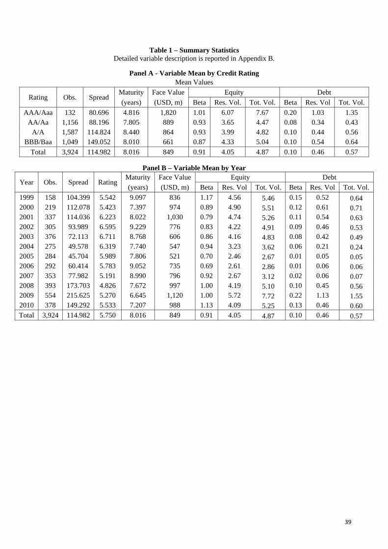
Table 1 – Summary Statistics Detailed variable description is reported in Appendix B.

Panel A - Variable Mean by Credit Rating Mean Values

Rating Obs. Spread Maturity Face Value Equity Debt (years) (USD, m) Beta Res. Vol. Tot. Vol. Beta Res. Vol Tot. Vol.

AAA/Aaa 132 80.696 4.816 1,820 1.01 6.07 7.67 0.20 1.03 1.35 AA/Aa 1,156 88.196 7.805 889 0.93 3.65 4.47 0.08 0.34 0.43

A/A 1,587 114.824 8.440 864 0.93 3.99 4.82 0.10 0.44 0.56 BBB/Baa 1,049 149.052 8.010 661 0.87 4.33 5.04 0.10 0.54 0.64

Total 3,924 114.982 8.016 849 0.91 4.05 4.87 0.10 0.46 0.57

Panel B – Variable Mean by Year

Year Obs. Spread Rating Maturity Face Value Equity Debt (years) (USD, m) Beta Res. Vol Tot. Vol. Beta Res. Vol Tot. Vol.

1999 158 104.399 5.542 9.097 836 1.17 4.56 5.46 0.15 0.52 0.64 2000 219 112.078 5.423 7.397 974 0.89 4.90 5.51 0.12 0.61 0.71 2001 337 114.036 6.223 8.022 1,030 0.79 4.74 5.26 0.11 0.54 0.63 2002 305 93.989 6.595 9.229 776 0.83 4.22 4.91 0.09 0.46 0.53 2003 376 72.113 6.711 8.768 606 0.86 4.16 4.83 0.08 0.42 0.49 2004 275 49.578 6.319 7.740 547 0.94 3.23 3.62 0.06 0.21 0.24 2005 284 45.704 5.989 7.806 521 0.70 2.46 2.67 0.01 0.05 0.05 2006 292 60.414 5.783 9.052 735 0.69 2.61 2.86 0.01 0.06 0.06 2007 353 77.982 5.191 8.990 796 0.92 2.67 3.12 0.02 0.06 0.07 2008 393 173.703 4.826 7.672 997 1.00 4.19 5.10 0.10 0.45 0.56 2009 554 215.625 5.270 6.645 1,120 1.00 5.72 7.72 0.22 1.13 1.55 2010 378 149.292 5.533 7.207 988 1.13 4.09 5.25 0.13 0.46 0.60 Total 3,924 114.982 5.750 8.016 849 0.91 4.05 4.87 0.10 0.46 0.57

39 

 

Table 2 – Mean Credit Spreads by Credit Ratings – High vs. Low Systematic Risk This table reports the mean Spread for bonds with different ratings and maturity. Bonds are split according to their Equity Beta (Panel A) and Debt Beta (Panel B). Detailed variable description is reported in Appendix B. ***, **, * indicate statistical significance (1%, 5%, 10%, respectively) of the t-test for the equality of the mean Spread for bonds with beta below and above the median.

Panel A – Equity Beta All Issues (3,924 Bonds)

Maturity Equity Beta below median (0.867) Equity Beta above median (0.867) AA A BBB Total AA A BBB Total

≤ 10 years 66.78 93.25 125.28 95.06 106.52*** 130.14*** 166.88*** 132.55*** > 10 years 71.16 115.44 175.29 116.36 124.23*** 148.69*** 191.19 149.92***

Total 67.48 96.86 131.67 98.28 108.14*** 131.97*** 168.66*** 134.11*** Excluding 2008-10 (2,599 Bonds)

Maturity Equity Beta below median (0.799) Equity Beta above median (0.799)

AA A BBB Total AA A BBB Total ≤ 10 years 47.00 69.88 83.19 68.09 67.62*** 85.65*** 91.258* 82.36*** > 10 years 70.78 107.37 108.62 96.40 101.98*** 113.08 184.20*** 127.72***

Total 51.05 76.10 85.99 72.34 72.07*** 88.84*** 100.50*** 87.58***

Panel B – Debt Beta All Issues (3,924 Bonds)

Maturity Debt Beta below median (0.038) Debt Beta above median (0.038)

AA A BBB Total AA A BBB Total ≤ 10 years 65.68 77.47 119.45 84.19 114.11*** 144.87*** 165.86*** 143.04*** > 10 years 73.55 108.80 167.84 110.49 128.36*** 162.52*** 202.070* 162.59***

Total 66.87 82.68 126.19 88.25 115.40*** 146.53*** 168.41*** 144.72*** Excluding 2008-10 (2,599 Bonds)

Maturity Debt Beta below median (0.020) Debt Beta above median (0.020) AA A BBB Total AA A BBB Total

≤ 10 years 51.22 64.86 85.06 64.98 67.84*** 90.48*** 88.44 85.05*** > 10 years 74.18 100.17 131.21 96.94 106.71*** 124.740** 156.027* 129.90***

Total 55.01 70.91 91.24 70.11 72.68*** 94.26*** 94.34 89.75***

40 

 

41 

Table 3 - Bond Spreads by Currency Denomination and Debt Beta Quartile

This table reports spreads for bonds of different currency denominations and different rating classes, sorted by quartiles of the issuer’s debt beta. Quartile 1 contains the 25% of bonds of the given rating class whose issuers have the lowest debt beta (systematic risk) while quartile 4 is the 25% of bonds whose issuers have the highest debt beta. Because each rating class contains three notches (+, flat, -), the reported average Spread in a given quartile is adjusted to represent the mean notch rating for the class. Details of this regression-based adjustment are given in the text. ***, **, * indicate statistical significance (1%, 5%, 10%, respectively) of the t-test for the equality of the adjusted spreads of bonds in the first and fourth debt beta quartiles.

Average Euro Denominated Bond Spreads

(in basis points)

Debt Beta Quartile Rating AA A BBB

1 52.22 83.20 123.73 2 89.48 107.40 146.93 3 121.66 170.89 214.59 4 145.03*** 210.22*** 320.15***

Total Observations 304 492 346 Average US Dollar Denominated Bond Spreads

(in basis points)

Debt Beta Quartile Rating AA A BBB

1 79.98 114.93 262.75 2 105.54 147.98 252.79 3 126.84 191.29 200.43 4 141.93*** 197.83*** 336.89**

Total Observations 349 432 164 Average Japanese Yen Denominated Bond Spreads

(in basis points)

Debt Beta Quartile Rating AA A BBB

1 18.87 22.79 34.77 2 18.96 23.61 38.15 3 23.61 29.20 39.05 4 35.94*** 37.80*** 44.73***

Total Observations 246 434 403 Average British Pound Denominated Bond Spreads

(in basis points)

Debt Beta Quartile Rating AA A BBB

1 60.00 101.75 157.06 2 68.19 105.73 159.29 3 109.98 168.01 202.06 4 138.19*** 172.66*** 311.75***

Total Observations 152 164 115

 

42 

Table 4 – Debt Beta of Bonds with High Spreads Sample bonds are categorized by year of issuance, currency (Euro, US Dollar, and Yen), and credit rating. For each category with at least five issues, bonds are ranked based on their credit spreads and the average debt beta is computed for All of the bonds in the category versus only those bonds with Spreads Above the Median. (high-spread bonds). This table reports the mean Debt Beta. Panel A reports debt beta values for bonds with maturities of 10 years and less while Panel B reports debt beta values for bonds with maturities greater than 10 years. Values in bold indicate that the mean debt beta for high-spread bonds is greater than mean debt beta for all bonds in the category.

Panel A –Years to Maturity ≤ 10 years Year Sub-sample EUR USD JPY

AAA-AA A BBB AAA-AA A BBB AAA-AA A BBB 1999 Spread above Median 0.224 0.158 0.158 0.228 0.189 0.232 0.123 0.060

All 0.219 0.142 0.145 0.142 0.161 0.150 0.064 0.060 2000 Spread above Median 0.057 0.110 0.046 0.192 0.247 0.180 0.268 0.110

All 0.062 0.099 0.063 0.144 0.177 0.187 0.203 0.105 2001 Spread above Median 0.099 0.151 0.187 0.166 0.202 0.196 0.208 0.112 0.099

All 0.070 0.114 0.127 0.100 0.155 0.150 0.130 0.070 0.104 2002 Spread above Median 0.190 0.126 0.254 0.064 0.087 0.055 0.033 0.033 0.144

All 0.098 0.138 0.185 0.047 0.061 0.102 0.020 0.053 0.109 2003 Spread above Median 0.092 0.192 0.233 0.042 0.102 0.230 0.034 0.061 0.078

All 0.077 0.133 0.157 0.039 0.093 0.130 0.034 0.070 0.072 2004 Spread above Median 0.025 0.018 0.067 0.006 0.031 0.019 0.044 0.134

All 0.014 0.033 0.039 0.004 0.021 0.014 0.101 0.121 2005 Spread above Median 0.002 0.014 0.010 0.002 0.011 0.003 0.005 0.010 0.048

All 0.002 0.008 0.008 0.001 0.006 0.008 0.004 0.012 0.033 2006 Spread above Median 0.006 0.005 0.009 0.002 0.005 0.091 0.017 0.038 0.032

All 0.003 0.004 0.007 0.001 0.003 0.065 0.012 0.034 0.024 2007 Spread above Median 0.021 0.013 0.006 0.019 0.022 0.062 0.045 0.054 0.073

All 0.014 0.012 0.007 0.012 0.015 0.040 0.030 0.042 0.047 2008 Spread above Median 0.099 0.106 0.069 0.090 0.093 0.015 0.097 0.140 0.336

All 0.120 0.078 0.042 0.181 0.061 0.039 0.073 0.152 0.260 2009 Spread above Median 0.242 0.254 0.295 0.221 0.413 0.218 0.138 0.241 0.371

All 0.237 0.231 0.265 0.244 0.361 0.135 0.138 0.233 0.370 2010 Spread above Median 0.189 0.119 0.137 0.180 0.178 0.255 0.073 0.073 0.117

All 0.152 0.121 0.112 0.133 0.169 0.172 0.059 0.083 0.117

 

43 

Panel B - Maturity > 10 years Year Sub-sample EUR USD JPY

AAA-AA A BBB AAA-AA A BBB AAA-AA A BBB 1999 Spread above Median 0.195

All 0.124 2000 Spread above Median 0.216

All 0.147 2001 Spread above Median 0.124

All 0.156 2002 Spread above Median 0.147 0.010 0.034

All 0.117 0.032 0.026 2003 Spread above Median 0.175 0.101 0.102 0.034

All 0.139 0.072 0.087 0.037 2004 Spread above Median 0.012 0.041

All 0.016 0.026 2005 Spread above Median 0.000 0.002 0.082

All 0.000 0.002 0.091 2006 Spread above Median 0.009 0.003 0.015 0.043

All 0.007 0.002 0.016 0.040 2007 Spread above Median 0.010 0.017 0.007 0.030 0.072

All 0.006 0.011 0.014 0.020 0.061 2008 Spread above Median 0.094 0.110 0.057 0.038 0.167

All 0.071 0.060 0.035 0.026 0.114 2009 Spread above Median 0.099 0.082 0.309 0.204 0.329 0.154

All 0.084 0.054 0.192 0.201 0.239 0.100 2010 Spread above Median 0.173 0.091 0.115 0.006

All 0.092 0.045 0.082 0.010

 

Table 5 – Average Beta of Bonds with High Spreads – t-test For each category reported in Table 4 we compute the ratio of the average beta of high-spread bonds to the average beta of all the bonds within the same category. This table reports the mean log ratios. ***, **, * indicate statistical significance (1%, 5%, 10%, respectively) of the t-test for the equality of the mean log ratios to zero.

Maturity EUR USD JPY Total ≤ 10 years 0.190*** 0.183*** 0.129*** 0.169*** > 10 years 0.341*** 0.219*** 0.108 0.201***

Total 0.212*** 0.196*** 0.123*** 0.178***

44 

 

Table 6 – Regression of Credit Spread on Ratings and Debt Systematic Risk Reported are coefficients of OLS regressions with robust standard errors clustered both at the year and issuer level. The dependent variable is Spread, i.e. the difference between the bond yield at issuance and that of a Treasury security with same maturity and currency. Detailed variable description is reported in Appendix B. Coefficient for control variables are not reported for ease of exposition. ***, **, * indicate significance at 1%, 5%, 10% level, respectively.

(1) (2) (3) (4) (5)

Whole Sample Excluding 08-10 Whole

AA+/Aa1 73.641*** 82.059*** 82.158*** 3.797 75.990***

(0.000) (0.000) (0.000) (0.826) (0.001)

AA/Aa2 83.889*** 92.379*** 92.150*** 5.477 81.549***

(0.000) (0.000) (0.000) (0.648) (0.001)

AA-/Aa3 109.311*** 111.737*** 111.650*** 17.742* 98.391***

(0.000) (0.000) (0.000) (0.057) (0.000)

A+/A1 117.662*** 119.570*** 119.276*** 21.217** 107.155***

(0.000) (0.000) (0.000) (0.015) (0.000)

A/A2 133.765*** 134.584*** 134.284*** 31.379*** 121.631***

(0.000) (0.000) (0.000) (0.000) (0.000)

A-/A3 152.259*** 154.257*** 153.903*** 42.027*** 139.632***

(0.000) (0.000) (0.000) (0.000) (0.000)

BBB+/Baa1 182.061*** 182.894*** 182.433*** 57.829*** 166.114***

(0.000) (0.000) (0.000) (0.000) (0.000)

BBB/Baa2 199.850*** 196.790*** 196.316*** 62.452*** 178.798***

(0.000) (0.000) (0.000) (0.000) (0.000)

BBB-/Baa3 211.318*** 208.639*** 208.109*** 76.344*** 188.046***

(0.000) (0.000) (0.000) (0.000) (0.000)

Debt Beta 108.781*** 105.424*** 67.799*** 41.618** (0.000) (0.001) (0.000) (0.045)

ln (Debt Residual Volatility) 0.432 0.803 2.555 (0.831) (0.419) (0.103)

Crisis (2008-10) 93.842*** (0.000)

Debt Beta × Crisis 228.267*** (0.002)

Obs. 3,924 3,924 3,924 2,599 3,924 Adj. R2 0.610 0.623 0.623 0.642 0.601

45 

 

Table 7 – Regression of Credit Spread on Ratings and Debt Systematic Risk (Bid-Ask Spread)

Reported are coefficients of OLS regressions with robust standard errors clustered both at the year and issuer level. The dependent variable is Spread, i.e. the difference between the bond yield at issuance and that of a Treasury security with same maturity and currency. Detailed variable description is reported in Appendix B. Coefficient for control variables are not reported for ease of exposition. ***, **, * indicate significance at 1%, 5%, 10% level, respectively.

(1) (2) (3) (4) (5)

Whole Sample Excluding 08-10 Whole

AA+/Aa1 87.790** 100.594** 100.418** -4.890 92.318** (0.016) (0.011) (0.011) (0.726) (0.020)

AA/Aa2 99.555*** 113.670*** 114.855*** 3.097 104.580***

(0.006) (0.003) (0.004) (0.731) (0.008)

AA-/Aa3 119.208*** 129.359*** 130.239*** 13.445* 117.376***

(0.003) (0.002) (0.002) (0.063) (0.008)

A+/A1 119.658*** 128.089*** 129.438*** 16.726** 119.009***

(0.002) (0.002) (0.002) (0.018) (0.006)

A/A2 137.262*** 143.876*** 145.402*** 24.437*** 135.210***

(0.001) (0.001) (0.001) (0.000) (0.003)

A-/A3 146.725*** 153.758*** 155.407*** 37.334*** 142.834***

(0.000) (0.000) (0.000) (0.000) (0.000)

BBB+/Baa1 169.333*** 174.518*** 176.557*** 55.574*** 162.262***

(0.000) (0.000) (0.000) (0.000) (0.000)

BBB/Baa2 190.508*** 191.277*** 193.208*** 57.731*** 179.135***

(0.000) (0.000) (0.000) (0.000) (0.000)

BBB-/Baa3 206.119*** 207.675*** 209.928*** 88.358*** 192.440***

(0.000) (0.000) (0.000) (0.000) (0.000)

Debt Beta 131.123*** 139.492*** 75.937*** 65.137*** (0.000) (0.000) (0.000) (0.001)

ln (Debt Residual Volatility) -1.185 -0.063 0.819 (0.513) (0.939) (0.578)

Crisis (2008-10) 106.996*** (0.000)

Debt Beta × Crisis 299.626*** (0.000)

Avg Bid-Ask Spread

103.655*** 89.896*** 90.439*** 61.144*** 112.314***(0.000) (0.000) (0.000) (0.000) (0.000)

Obs. 2,395 2,395 2,395 1,732 2,395 Adj. R2 0.641 0.659 0.659 0.662 0.637

46 

 

47 

Table 8 – Regression of Average Rating on Debt Systematic Risk

Reported are coefficients of OLS regressions (Columns 1-6) and ordered probit (Columns 7-8) with robust standard errors clustered both at the year and issuer level. The dependent variable is Avg_Rating, i.e. the average of Moody’s and S&P’s issue ratings, converted into numerical scale (AAA/Aaa = 1, AA-/Aa1 = 2, …, BBB-/Bbb3 = 10). Detailed variable description is reported in Appendix B. Coefficient for control variables are not reported for ease of exposition. ***, **, * indicate significance at 1%, 5%, 10% level, respectively.

(1) (2) (3) (4) (5) (6) (7) (8)

OLS Ordered Probit Whole Sample Excluding 2008-10

Debt Beta 1.875*** 0.917 0.883 2.947*** 1.682*** 1.627*** 1.259*** 1.219***(0.006) (0.202) (0.218) (0.000) (0.002) (0.003) (0.000) (0.000)

ln (Debt Residual Volatility) 0.123*** 0.155*** 0.109*** (0.000) (0.000) (0.000)

ln (Debt Total Volatility) 0.121*** 0.153*** 0.108*** (0.000) (0.000) (0.000)

Obs. 3,924 3,924 3,924 2,599 2,599 2,599 2,599 2,599 Adj. R2 0.474 0.482 0.481 0.523 0.537 0.537 0.186 0.186

 

Table 9 – Moody’s vs. S&P’s ratings Reported are coefficients of OLS regressions (Columns 1-8) and probit regressions (Column 9-12) with robust standard errors clustered both at the year and issuer level. In Columns 1-4 the dependent variable is the rating of Moody’s (Columns 1-2 and 5-6) or S&P’s (Columns 3-4 and 7-8) converted into a numerical scale (AAA/Aaa = 1, AA+/Aa1 = 2, …, BBB-/Bbb3 = 10). In Columns 9-12 the dependent variable is Split, that is equal to 1 if Moody’s and S&P’s ratings for the same issue are different, zero otherwise. Detailed variable description is reported in Appendix B. Coefficient for control variables are not reported for ease of exposition. ***, **, * indicate significance at 1%, 5%, 10% level, respectively.

(1) (2) (3) (4) (5) (6) (7) (8) (9) (10) (11) (12)

Whole Sample Excluding 2008-10 Whole Sample Excluding 2008-10 Moody's S&P's Moody's S&P's Split

Debt Beta 0.664 0.631 0.553 0.527 1.527*** 1.451*** 1.441*** 1.391** -1.033*** -1.004*** -1.554** -1.531*

(0.494) (0.516) (0.472) (0.493) (0.002) (0.005) (0.008) (0.012) (0.003) (0.004) (0.048) (0.053) ln (Debt Residual

Volatility) 0.136*** 0.128*** 0.190*** 0.160*** -0.015 -0.013 (0.002) (0.000) (0.000) (0.000) (0.426) (0.666)

ln (Debt Total Volatility)

0.134*** 0.126*** 0.188*** 0.158*** -0.019 -0.015 (0.002) (0.000) (0.000) (0.000) (0.304) (0.606)

Obs. 2,658 2,658 3,715 3,715 1,472 1,472 2,489 2,489 2,439 2,439 1,336 1,336 Adj. R2 0.523 0.523 0.475 0.475 0.564 0.564 0.538 0.538 0.230 0.231 0.234 0.234

 

48