Banking, Liquidity E¤ects, and Monetary Policy

Te-Tsun ChangNational Chi-Nan University

Yiting Li�

National Taiwan University

January 2016

Abstract

We study liquidity e¤ects and monetary policy in a model with fully �exible prices and ex-plicit roles for money and �nancial intermediation. Banks hold some fractions of deposits andmoney injections as liquidity bu¤ers. The higher the fraction kept as reserves, the less liquidmoney is. Unexpected money injections raise output and lower nominal interest rates i¤ thenewly injected money is more liquid than the initial money stocks. If banks hold no liquiditybu¤ers, liquidity e¤ects are eliminated. In an extended model with temporary shocks, we showthat, contrary to Berentsen and Waller (2011), failure to withdraw state-contingent money injec-tions does not make the stabilization policy neutral, though the economy may undergo highershort-run �uctuations than otherwise. Under this circumstance, the success of stabilizationpolicy relies on unexpected money injections being more liquid than the initial money stock.

JEL Classi�cation: E41; E50Keywords: Liquidity e¤ects; Money; Banking; Credit; Interest rates; Monetary policy

�Corresponding author. Yiting Li, Department of Economics, National Taiwan University, No. 1, Sec. 4, RooseveltRoad, 10617 Taipei, Taiwan. E-mail: yitingli@ntu.edu.tw. Te-Tsun Chang: ttchang@ncnu.edu.tw. We thank twoanonymous referees for comments and suggestions that substantially improved the paper. We also thank JonathanChiu, Kevin X.D. Huang, Young Sik Kim and Shouyong Shi for helpful comments on the earlier draft of the paper,and participants in the 2014 Econometric Society Asian Meetings in Taipei for helpful comments and conversations.

1 Introduction

In a world where people are subject to trading shocks, banks can play an e¢ ciency role by channeling

funds from people with idle money to those who are cash constrained. This role, however, is

limited by banks�holding reserves, due to regulations and liquidity management considerations.1

For instance, the recent Basel III proposal requires that banks hold liquidity bu¤ers sizeable enough

to enable them to withstand a severe short-term shock.2 Banks� liquidity bu¤ers may a¤ect the

monetary transmission mechanism and the conduct and e¤ectiveness of monetary policy. To explore

the potential e¤ects, we use a general equilibrium framework with frictions, which give rise to the

roles of money and �nancial intermediation (see, e.g., Lagos and Wright 2005, and Berentsen,

Camera, and Waller 2007).

In this economy, banks take deposits from people with idle cash and lend to those who need

liquidity to �nance unanticipated consumption. The central bank injects money through �nancial

intermediaries. Agents make decisions about money holdings before they learn the shocks of pref-

erences and money injections. The preference shock determines whether an agent is a seller or a

buyer. Sellers deposit idle cash whereas buyers can borrow money from banks. Fiat money is used

as the medium of exchange, due to limitations on record keeping, enforcement, and commitment.

Agents, however, are not subject to the standard cash-in-advance constraint because, before trad-

ing, they can borrow cash from banks to replenish their money holdings. The amount that agents

can borrow is a¤ected by banks�holdings of liquidity bu¤ers. Banks hold (di¤erent) fractions of

deposits and newly injected money as reserves. Money kept as bank reserves does not provide

liquidity to lubricate economic activity, and the higher the fraction kept as reserves, the less liquid

money is.

An unexpected money injection results in two e¤ects in the economy: it increases the nominal

amount of loans (loanable funds e¤ect), and it also raises in�ation expectations (Fisher e¤ect). We1Requiring that banks hold su¢ ciently high liquid assets is a cost on �nancial intermediation. However, As

Freedman and Click (2006) and Ratnovski (2009) have argued, developing countries have to rely on the quantitativeliquidity regulation because of less available information on banks�net worth.

2The short-term liquidity bu¤er (mostly comprising cash, central bank reserves, and domestic sovereign bonds),known as the liquidity coverage ratio, will require a bank to have enough highly liquid assets on the balance sheetto cover its net cash out�ows over a 30-day period following a shock, such as a three-notch downgrade to its publiccredit rating. This requirement will come into e¤ect in 2015. See Basel III: International framework for liquidity riskmeasurement, standards and monitoring, December 2010.

1

�nd that unexpected money injections raise output and reduce nominal interest rates if and only

if the fraction of money injections used to �nance spending is larger than the fraction of the initial

money stock used to �nance spending; i.e., when the injected money is more liquid than the initial

money stock. This condition implies that the loanable funds e¤ect outweighs the Fisher e¤ect,

increasing buyers�real balances. The lower nominal interest rates also stimulate borrowing, leaving

higher total liquidity to support economic activity. Note that if the money injection is anticipated,

it always raises nominal interest rates and generates no liquidity e¤ect.

If the newly injected cash is as liquid as the initial money stock (e.g., banks hold no liquidity

bu¤ers), the liquidity e¤ect is eliminated. This is so because agents�decisions on money holdings

are in line with any money growth rate. Consequently, unexpected money injections do not dis-

tort anything, and agents make portfolio decisions as if they knew the amount of future money

injections. Thus, in contrast to the previous literature, though agents make portfolio choices before

the realization of monetary shocks, the informational friction in our model does not necessarily

generate a liquidity e¤ect.3

After establishing the monetary transmission mechanism in the basic model, we �rst extend

it by incorporating temporary demand shocks to study optimal monetary policy. In the second

extension we motivate banks�holding reserves by resorting to the need for liquidity management

due to random deposit withdrawals. Our analysis shows that in conducting stabilization policy, the

central bank needs to weigh the payo¤ to managing in�ation expectations against the e¤ectiveness

of implementing policy, measured by the magnitude of a liquidity e¤ect. In an economy with high

level of economic activity, it does little good to raise money injections (and therefore, in�ation

expectations) to increase consumption, whereas its small liquidity e¤ect requires higher money

injections to achieve the goal. When aggregate demand is high, the central bank weighs less on the

risk of raising in�ation expectations, and thus, it injects more money in an economy with higher

economic activity than otherwise; the opposite occurs when aggregate demand is low. It is thus

observed that the central bank reacts to shocks more aggressively in an economy with a relatively

high level of economic activity.

3For instance, Lucas (1990), Christiano (1991) and Fuerst (1992) attribute the source of the liquidity e¤ect toa type of information friction that arises because agents are not able to adjust their portfolios at the time moneyinjections take place.

2

Our extended model is similar to Berentsen and Waller (2011); however, in their model lenders

do not hold liquidity bu¤ers. In Berentsen and Waller (2011), the critical element for e¤ective

stabilization policy is the central bank�s price-level targeting policy, which will undo the current

money injections at a future date. In the current paper failure to withdraw money injections does

not make the stabilization policy neutral, though the economy undergoes higher �uctuations than

otherwise. The management of in�ation expectations is di¤erent under the two policy regimes.

Under the price-level targeting policy studied by Berentsen and Waller (2011), the central bank

controls long-run in�ation expectations; in our model where the central bank lacks the ability

to withdraw the state-contingent money injections at a speci�ed future date, it must at least

commit itself to a short-run expected in�ation to implement the stabilization policy. Under this

circumstance, the existence of a liquidity e¤ect and the success of stabilization policy rely on

unexpected money injections being more liquid than the initial money stock.

The rest of the paper is organized as follows. Section 2 describes the basic model. Section

3 derives equilibrium conditions. In section 4 we study the liquidity e¤ect and discuss further

what distinguishes our paper from the literature. Section 5 illustrates some extensions of the basic

model. We conclude in section 6. All proofs and omitted derivations of equations are contained in

the Appendix.

2 The basic model

The environment is based on Lagos and Wright (2005) and Berentsen, Camera, and Waller (2007).

There is a [0; 1] continuum of in�nitely lived agents. Time is discrete and continues forever. Each

period is divided into two subperiods, and in each subperiod trades occur in competitive markets.

There are perishable and perfectly divisible goods, one produced in the �rst subperiod, and the

other (called the general good) in the second subperiod. The discount factor across periods is

� = 11+� 2 (0; 1); where � is the rate of time preference.

In the beginning of the �rst subperiod, an agent receives a preference shock that determines

whether he consumes or produces. With probability � an agent can consume but cannot produce;

with probability 1�� the agent can produce but cannot consume. We refer to consumers as buyers

and producers as sellers. This is a simple way to capture the uncertainty of the opportunity to

3

trade. Consumers get utility u(q) from q consumption, where u0(q) > 0, u00(q) < 0, u0(0) = 1

and u0(1) = 0. Producers incur disutility c(q) from producing q units of output, where c0(q) > 0,

c00(q) � 0. To motivate a role for �at money, we assume that all goods trades are anonymous, and

there is no public record of individuals�trading histories.

In the second subperiod, all agents can produce and consume the general good, getting utility

U(x) from x consumption, where U 0(x) > 0, U 00(x) � 0, U 0(0) = 1; and U 0(1) = 0. Agents can

produce one unit of the general good with one unit of labor, which generates one unit of disutility.

This setup allows us to introduce an idiosyncratic preference shock while keeping the distribution

of money holdings analytically tractable.

A government is the sole issuer of �at money. The evolution of the money stock is Mt = (1 +

zt)Mt�1, whereMt denotes the per capita currency stock, and zt is the money growth rate, in period

t: Assume zt = �+ "t, where � is the long-run money growth rate, and "t is a serially uncorrelated

random variable with the density function f on ["; "]: The random variable, "t; generates a monetary

shock, which becomes known at the beginning of period t: In the �rst subperiod, the central bank

injects money, � t = ztMt�1; or it can levy nominal taxes from banks�reserves to extract cash from

the economy, which implies � t < 0 and zt < 0.

Competitive banks accept nominal deposits and make nominal loans. Sellers in the �rst sub-

period can deposit their money holdings in banks at the nominal interest rate, id, and are entitled

to withdraw funds in the second subperiod. Buyers can borrow money from banks at the nominal

loan rate, i; and repay their loans in the second subperiod. We assume that loans and deposits are

not rolled over, and so all �nancial contracts are one-period contracts.4 Moreover, banks have zero

net worth, and there are no operating costs.

Banks keep records on �nancial histories but not on trading histories in the goods market.

The record-keeping technology is not available to individuals, so credit between private agents is

not feasible. We assume full enforcement of debt repayment, and so default is not possible.5 In

equilibrium, the loan rate i clears the loan market. Assume that banks are owned by private agents.

4With the assumption on the linear utility costs of production in the second subperiod, agents do not gain byspreading the repayment of loans or redemption of deposits across periods.

5But see, e.g., Berentsen, Camera, and Waller (2007) and Li and Li (2013), for considering the possibility ofdefault to study the e¤ects of in�ation on credit arrangements, output, and asset prices.

4

The central bank injects money through �nancial intermediaries, which extend funds to borrowers.

This transfer scheme is merely an analytical device to mimic open-market operations. Because

banks lend out money injected by the central bank, it is possible for competitive banks to obtain

positive pro�ts. A bank�s pro�ts are distributed to private agents as dividends, or are withdrawn

from agents�bank accounts in the case of zt < 0.

We consider an economy in which banks keep a bu¤er stock of reserves, due to liquidity risk

management considerations and regulations (see Section 4.2 for a more detailed discussion).6 Specif-

ically, we assume that banks lend out a constant fraction, � 2 (0; 1]; of deposits, and a fraction,

�m 2 (0; 1]; of money that the central bank injects into banks. In the basic model we treat �

and �m as parameters, and in Section 5 we consider random deposit withdrawals, in the spirit of

Diamond and Dybvig (1983), to justify banks�holding reserves.

The timing of events is summarized as follows. At the beginning of the �rst subperiod of period

t, each agent receives a preference shock, and money injections take place so that zt is known to

the public. Then sellers make deposits, buyers take loans, and they trade in the goods market.

In the second subperiod, agents settle �nancial claims, receive dividends from banks, and adjust

money holdings. In Section 5 we extend the basic model to incorporate demand shocks to discuss

stabilization policy, and introduce liquidity shocks to motivate banks�holding reserves, where we

will describe the time sequence in more details.

3 Equilibrium

Let �t denote the value of money in terms of the good produced in the second subperiod. We study

symmetric stationary equilibria in which end-of-period real balances are time-invariant; i.e., �tMt =

�t�1Mt�1: Thus,�t�1�t

= MtMt�1

= 1 + zt: As such, the money growth rate, zt; also represents the

in�ation rate in the second subperiod of period t: In the following discussions, to simplify notations

we let variables corresponding to the next period be indexed by +1; and variables corresponding

to the previous period be indexed by �1:

6A rationale for liquidity risk management is proposed by, for instance, Kashyap, Rajan, and Stein (2002): Banksprovide customers with liquidity on demand to satisfy their unexpected needs. Liquidity is provided by o¤eringdemand deposits and loan commitments, which give a borrower the option to take the loans on demand over a certainspeci�ed period of time. Both of these products require explicit liquidity risk management.

5

Let V (m) denote the expected value of entering the �rst subperiod with m units of money.

Let W (m; b; d) denote the expected value of entering the second subperiod with m units of money,

b debt, and d deposits, where loans and deposits are in the units of �at money. We study a

representative period t and work backwards from the second to the �rst subperiod, using a similar

approach as in Berentsen, Camera, and Waller (2007), to characterize equilibria.

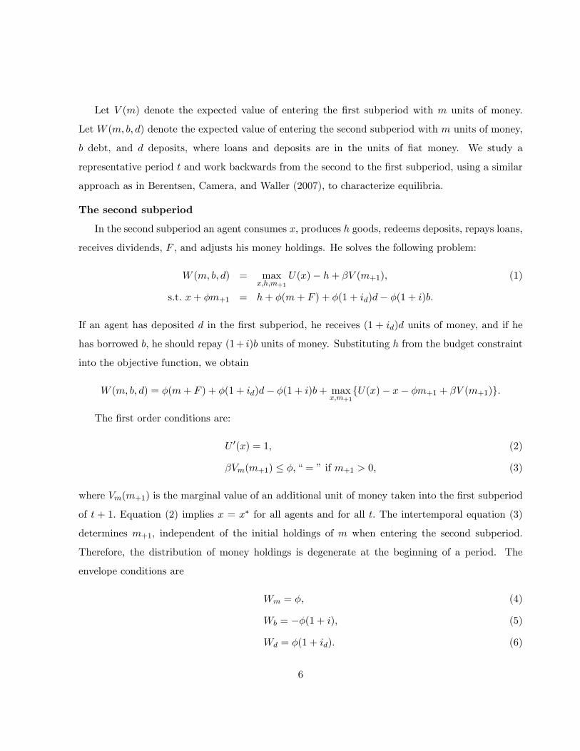
The second subperiod

In the second subperiod an agent consumes x; produces h goods, redeems deposits, repays loans,

receives dividends, F , and adjusts his money holdings. He solves the following problem:

W (m; b; d) = maxx;h;m+1

U(x)� h+ �V (m+1); (1)

s.t. x+ �m+1 = h+ �(m+ F ) + �(1 + id)d� �(1 + i)b:

If an agent has deposited d in the �rst subperiod, he receives (1 + id)d units of money, and if he

has borrowed b; he should repay (1+ i)b units of money. Substituting h from the budget constraint

into the objective function, we obtain

W (m; b; d) = �(m+ F ) + �(1 + id)d� �(1 + i)b+ maxx;m+1

fU(x)� x� �m+1 + �V (m+1)g:

The �rst order conditions are:

U 0(x) = 1; (2)

�Vm(m+1) � �;�= �if m+1 > 0; (3)

where Vm(m+1) is the marginal value of an additional unit of money taken into the �rst subperiod

of t + 1: Equation (2) implies x = x� for all agents and for all t: The intertemporal equation (3)

determines m+1; independent of the initial holdings of m when entering the second subperiod.

Therefore, the distribution of money holdings is degenerate at the beginning of a period. The

envelope conditions are

Wm = �; (4)

Wb = ��(1 + i); (5)

Wd = �(1 + id): (6)

6

The �rst subperiod

Let qb and qs denote the quantities consumed by a buyer and produced by a seller, respectively,

and p denote the nominal price of the good, in period t: Because agents trade in the goods market

after the monetary shock is realized, the price and quantities consumed and produced should depend

on the money injection; e.g., p(z) denotes the price when the money injection is z. For notational

simplicity we suppress the dependence of p on z: As well, we suppress the dependence of z for other

variables such as interest rates and quantity consumed and produced.

An agent may be a buyer with probability �; spending pqb units of money to get qb consumption,

or he may be a seller with probability 1��; receiving pqs units of money from qs production. Because

buyers do not make deposits and sellers do not take out loans, in what follows we let b denote loans

taken out by buyers and d denote deposits by sellers, and drop these arguments inW (m; b; d) where

relevant for notational simplicity. The expected utility of an agent from entering the �rst subperiod

of period t with money holdings m is

V (m) =

Zf�[u(qb) +W (m+ b� pqb; b)] + (1� �)[�c(qs) +W (m� d+ pqs; d)]g f(z)dz: (7)

Agents trade in a centralized market, so they take the price p as given. A seller solves

maxqs;d

�c(qs) +W (m� d+ pqs; d)

s.t. d � m:

Let �d denote the multiplier on the deposit constraint. The �rst order conditions are

�c0(qs) + pWm = 0;

�Wm +Wd � �d = 0:

Using (4) and (6) the �rst order conditions become

p =c0(qs)

�; (8)

�d = �id:

Equation (8) implies that a seller�s production is such that the marginal cost of production, c0(qs)� ,

equals the marginal revenue, p: For id > 0, the deposit constraint binds, and sellers deposit all

7

money balances; i.e., d = M�1: Moreover, the production qs is independent of the seller�s initial

portfolio brought to the �rst subperiod.

A buyer�s problem is

maxqb;b

u(qb) +W (m+ b� pqb; b)

s.t. pqb � m+ b:

The buyer faces the cash constraint that his spending cannot exceed his money holdings, m; plus

borrowing, b: He should have faced a constraint stating that his borrowing cannot exceed a certain

credit limit. However, because banks can force borrowers to repay loans at no cost, the borrowing

constraint does not bind; i.e., b � 1; and hence, we ignore this constraint. Let � be the multiplier

on the buyer�s cash constraint. Using (4), (5), and (8), the �rst order conditions are

u0(qb) = c0(qs)(1 +

�

�) (9)

�i = �: (10)

If � = 0, (9) reduces to u0(qb) = c0(qs); implying i = 0: If � > 0, the cash constraint binds, and the

buyer spends all of his money; i.e.,

qb =m+ b

p: (11)

Combining (9) and (10), we obtainu0(qb)

c0(qs)= 1 + i; (12)

which implies that buyers borrow up to the point at which the marginal bene�t of an additional

unit of borrowed money, u0(qb)c0(qs)

, equals the marginal cost, 1 + i:

To �nd an agent�s optimal money holdings, we take the derivative of value function in (7) with

respect to m; and use (4) and (6) to get the marginal value of money:

Vm(m) =

Z[�u0(qb)

p+ (1� �)�(1 + id)]f(z)dz: (13)

An agent receives u0(qb)p from spending the marginal unit of money as a buyer, and if he is a seller,

he deposits the idle cash in banks, which is valued �(1 + id) in the second subperiod. Using (3)

8

lagged one period to eliminate Vm(m) from (13), an agent�s optimal money holdings at period t�1

satisfy

�

Z[�u0(qb)

p+ (1� �)�(1 + id)]f(z)dz � ��1;�= �if m > 0: (14)

Condition (14) states that the cost of acquiring an additional unit of money must be greater than

the expected discounted bene�t, with the equality holding if agents choose to hold money.

In a symmetric equilibrium, the market clearing conditions for goods, money, and loan markets

are

(1� �)qs = �qb; (15)

m =M�1; (16)

�b = �(1� �)d+ �m� ; (17)

respectively. In the loan market clearing condition, (17), the loanable funds per capita include �

fraction of deposits, (1� �)d; and �m fraction of money injection, �m� t, while the loan demand is

�b:

Competitive banks accept nominal deposits and make nominal loans, and they take as given the

loan rate and the deposit rate. In this model, banks are also the channel through which the central

bank injects money into the economy. To ensure that a bank cannot become in�nitely pro�table

by attracting in�nitely large amount of funds, we have the following zero marginal pro�t condition:

�i = id; (18)

which is a result of the competition between numerous banks. (See Appendix A for the details on

deriving solutions to the bank�s problem.) Banks receive money injections, � , a fraction �m of which

is lent to buyers at the nominal loan rate i: In the second subperiod, banks receive repayments,

(1 + i)�m� ; which, together with the unloaned money injections, (1 � �m)� ; are distributed as

dividends, F; to agents who own the bank.7 That is, the bank dividend payments are

F = (1 + i�m)� :

7We follow Fuerst�s (1994) setup in which the monetary authority injects money as a �helicopter drop�onto allbanks, and therefore, in equilibrium banks may have positive pro�ts (see also, Christiano 1991). As argued by Fuerst(1994), if open-market operations were modeled, the gains of the loanable reserves would be exactly o¤set by the lossof the interest-bearing securities.

9

De�nition 1 A monetary equilibrium with credit is (p; �; i; qb); satisfying (8), (12), (14), and

� =�qbc

0( �1�� qb)

[�+(1��)�+�mz]M�1:8

3.1 The �rst-best allocation

In a stationary equilibrium, the expected life-time utility of the representative agent at the beginning

of period t is

(1� �)Ws = �u(qb)� (1� �)c(�

1� � qb) + U(x)� x:

Imagine that the social planner is destined to maximize the representative agent�s expected utility.

The �rst-best allocation, (x�; q�b ; q�s); thus satis�es

U 0(x�) = 1;

u0(q�b ) = c0(

�

1� � q�b ):

These are the quantities chosen by a social planner who could force agents to produce and consume.

4 The Liquidity E¤ect

In this section we derive conditions for the existence of a liquidity e¤ect� unexpected money in-

jections raise output and lower nominal interest rates� and then discuss di¤erences between the

current model and the literature.

4.1 Existence of a liquidity e¤ect

We �rst derive the total funds available per buyer to �nance consumption in the �rst subperiod.

The total funds include an agent�s money holdings, m; and the money borrowed from a bank, b:

From the loan market clearing condition, (17),

b =�(1� �)d+ �m�

�: (19)

8From (8), (11), and (17), pqb = m+b = m+�(1��)d+�m�

�= �m+�(1��)d+�m�

�: Substituting (8), d = m, � = zM�1,

and m =M�1 into the above expression, we obtain � =�qbc

0( �1�� qb)

[�+(1��)�+�mz]M�1:

10

Substituting d = m; � = zM�1; and the market-clearing condition for money, m =M�1; into (19),

we obtain the total funds available per buyer as

m+ b =(�+ �mz)

�M�1; (20)

where

� = � + (1� �)�:

Note that � and �m are the fractions of the initial money stock, M�1; and the newly injected

money, zM�1; respectively, that can be used to �nance spending in the �rst subperiod.

In the equilibrium where the cash constraint binds, qb = m+bp ; from which we derive the rela-

tionship between qb and the money injection, z :

qbc0(�qb1� � ) =

(�+ �mz)��1M�1�(1 + z)

; (21)

by using (8), (20), and 1 + z =��1� : Taking the derivative of (21) with respect to z; we obtain

@qb@z

=��1M�1(�m � �)

�(1 + z)2[c0( �qb1�� ) +�qb1�� c

00( �qb1�� )]

8<:> >= 0 i¤ �m � � = 0:< <

(22)

Observe from (22) that the existence of a liquidity e¤ect (@qb@z > 0) depends on the relative

magnitudes of �m and �: The intuitive reason is as follows. Money kept as banks�reserves does

not provide liquidity to lubricate economic activity. For instance, when less of the bank�s deposits

are lent out, � is smaller, which implies that the fraction of the initial money stock used to �nance

spending is lower. One can interpret � and �m as the liquidity parameters for the initial money

stock and newly injected money, respectively. Intuitively, (22) says if the central bank injects

money which is more liquid than the initial money stock (�m > �); total liquidity rises to support

economic activity, and therefore, output rises.

The necessary condition for �m > � is that the fraction of deposits banks lend out, �; is less than

�m: Central banks usually impose reserve requirements against speci�ed deposit liabilities, and so

� < 1; while no such requirements on reserves that banks acquire from open market operations.9

9The Fed imposes reserve requirements against speci�ed deposit liabilities. For instance, net transac-tion accounts in excess of the low-reserve tranche are currently reservable at 10 percent. For details, seehttp://www.federalreserve.gov/monetarypolicy/reservereq.htm.

11

In our model, the injection of money is as a �helicopter drop� onto all banks, which is a simple

way to mimic open market operations. The interests lost from selling interest-bearing securities

to the central bank must be o¤set by the interests earned from lending out reserves. Therefore, a

bank may well lend out money injected, and �m = 1. In sum, banks do not lend out all deposits

due to liquidity risk management and regulations, whereas often no such considerations for money

injected by the central bank, which implies �m > �:10

To see more clearly the mechanism underlying the existence of a liquidity e¤ect, note that an

unexpected money injection results in two opposite e¤ects: it increases the nominal amount of

loans (loanable funds e¤ect), and it also raises in�ation expectations and lowers the future value

of money (Fisher e¤ect). A liquidity e¤ect exists if the loanable funds e¤ect outweighs the Fisher

e¤ect, and thus, leads to higher real balances to �nance spending. To illustrate this point, consider

a case with a linear cost function, c0(qs) = 1: This implies p = 1� from (8), and thus, the in�ation

rate in the �rst subperiod, pp�1; rises one-for-one with the in�ation rate in the second subperiod,

��1� : We rewrite (21) as

�qb =�(1 + �m

� z)��1M�1

1 + z: (23)

The right side of (23) is a buyer�s real balances, adjusted by the second subperiod�s in�ation rate,

1+z: From (23), if �m > �, an increase in z causes a stronger loanable funds e¤ect, which dominates

the Fisher e¤ect, raising a buyer�s real balances to support higher consumption.11

When output rises in response to unexpected money injections, interest rates fall. From (12)

and (15), u0(qb) = c0( �qb1�� )(1 + i): Thus, given u00 < 0 and c00 � 0; i falls as qb rises. Note that �

and �m a¤ect not only the existence but also the magnitude of the liquidity e¤ect. Equation (22)

shows that the magnitude of the liquidity e¤ect, measured by @qb@z ; increases in �m and decreases

10Though we can infer that in usual time �m > �; it is not easy, if not impossible, to �nd the magnitudes of �(and therefore, �) and �m from data. The recent �nancial crisis, however, may present a case in which �m < �:E¤ective October 1, 2008, the Federal Reserve Banks pay interest on required reserve balances and on excess reservebalances. This would increase banks�incentives to hold reserves, and reduce �m (in this model, however, the centralbank does not pay interest on banks�reserves). As mentioned by Cochrance (2014), during the last few years theFed has bought about $3trillion of assets, and created about $3 trillion of bank reserves, in which required reservesare only about $80 billion. Banks only held about $50 billion of reserves before the crisis. Thus, he concluded thatalmost all of the $3 trillion were excess reserves, held voluntarily by banks. One can interpret this case as �m beingextremely small, and we may well have �m < �:

11This is so even if the �rst subperiod�s in�ation rises more than the second subperiod�s in�ation, as in the casewith convex cost functions. The increase in the price, p; is in line with the seller�s incentive to produce more.

12

in �: The larger the di¤erence between �m and �; the stronger the liquidity e¤ect.12

From (22), when � = �m; the liquidity e¤ect is eliminated. That is, an increase in the money

growth rate does not a¤ect output and interest rates, a prediction which is di¤erent from the

previous literature with trade frictions. Though agents make portfolio choices before the realization

of money injections, their decisions on money holdings are in line with any z; as long as they can

borrow, and newly injected cash is as liquid as the initial money stock. In this case, unexpected

money injections do not distort anything. That is, agents make portfolio decisions as if they knew

the amount of future money injections. Thus, in contrast to the previous literature, the information

friction in our model does not necessarily generate a liquidity e¤ect.

We emphasize that money injections must be unanticipated to generate the liquidity e¤ect. By

contrast, if the money growth rate is known when agents choose money holdings, an increase in

the money growth rate reduces output. To see this, let denote the money growth rate in period

t; which is known when agents choose money holdings in t� 1: Removing the expectation operator

from (14) and using the stationary condition,��1� = 1 + ; we obtain the condition on optimal

money holdings in t� 1 as

1 +

�= �

u0(qb)

c0( �qb1�� )+ (1� �)[( u

0(qb)

c0( �qb1�� )� 1)� + 1]; (24)

From (24), the period-t output, qb; is pinned down by the anticipated money growth rate, ; and

an increase in reduces output, as is predicted in previous studies that also assume uncertainty

in trading opportunities (e.g., Lagos and Wright 2005).13 On the contrary, the decision on money

holdings described by (14) in period t�1 implies that, given the distribution of z; an agent chooses

12From (23) we derive a version of the equation of exchange by using ��1M�1 = �M :

p�qb =�(1 + �m

�z)

(1 + z)M:

The left side of the above equation is the aggregate demand for goods, and in the right side,�(1+

�m�z)

(1+z)is the velocity

of money. If �m > �; a money injection raises the velocity, leading to higher output and prices.13Using (12) we rewrite (24) as

1 +

�= 1 + �i;

which is the Fisher equation, but in our model, the nominal interest rate is also in�uenced by the liquidity parameter,�: An increase in increase the nominal interest rate, which is the in�ation expectation e¤ect as predicted by theFisher question, and there is no liquidity e¤ect.

13

his money holdings to the point where the expected discounted bene�t of holding an additional

unit of money must equal its cost. Once there is an unanticipated increase in money injections in

period t; the buyer�s real balances increase if �m > �; and consequently, output rises and nominal

interest rates fall.

We summarize our main results as follows.

Proposition 1 If banks hold liquidity bu¤ers, unexpected money injections raise output and lower

nominal interest rates if and only if the fraction of injected money used to �nance spending is larger

than the fraction of the initial money stock used to �nance spending (�m > �). If banks hold no

liquidity bu¤ers (� = �m = 1), the liquidity e¤ect is eliminated.

4.2 Discussion

We discuss distinctions between the current paper and the literature. The mechanism underlying

the liquidity e¤ect in our paper is similar to that in Williamson�s (2004) model with segmented

markets. Unanticipated money injections in Williamson�s model cause a redistribution of wealth

between shoppers in the cash-goods market and the credit-goods market, because households cannot

reallocate the newly issued �at money between the two markets. If the issuance of private money is

permitted, then after they learn the shock of money injections, households can issue private money

and reallocate it to cash shoppers, which eliminates the liquidity e¤ect. In our model, banks�

lending of injected cash is similar to the private money issuance in Williamson�s model, which

e¤ectively removes the cash-in-advance constraint. While Williamson (2004) assumes �at money

and privately issued money are perfect substitutes, which is similar to the case with � = �m in our

model, we go a step further to identify how di¤erent liquidity properties between the newly issued

money and the initial money stock a¤ect the existence and magnitude of the liquidity e¤ect.14

In Berentsen and Waller (2011) stabilization policy works through a liquidity e¤ect. In their

model, lenders do not hold liquidity bu¤ers, and the central bank injects money in response to

temporary aggregate shocks. We use a two-subperiod setup to illustrate the mechanism of their

14Previous literature using limited participation models to study liquidity e¤ects includes, for example, Grossmanand Weiss (1983), Rotemberg (1984), and Williamson (2006). They identify the distributional e¤ect of moneyinjections as the underlying mechanism, but often the models are not analytically tractable, except Williamson(2006).

14

model. Consider the example with a linear cost function, c0(qs) = 1; and so p = 1� : Recall that

z = �+", where � is the long-run money growth rate, and " is the state-contingent money injection

in period t: The price-level targeting policy implies that the central bank injects zM�1 in the �rst

subperiod, while withdraws "M�1 in the second subperiod so that MM�1

=��1� = 1 + �: Thus,

p = 1+���1

= (1 + �)p�1; i.e., the current price depends on the long-run money growth rate and last

period�s price. Using p = 1+���1

; we express the buyer�s binding budget constraint, pqb = m+ zM�1;

as

qb =1 + �+ "

1 + ���1M�1: (25)

The right side of (25) is the buyer�s real balances in the �rst subperiod, which is raised by the state-

contingent money injection, ": The price-level targeting policy implies that state-contingent money

injections do not cause in�ation in the second subperiod when sellers will spend. Consequently,

sellers are willing to produce more, while buyers�real balances increase to support higher consump-

tion. It is observed from (25) that, the promise of the central bank to undo state-contingent money

injection is key to the existence of a liquidity e¤ect and the e¤ectiveness of stabilization policy, for

otherwise, qb = ��1M�1.

A liquidity e¤ect exists in our model as long as �m > �; and failure to withdraw money injections

does not eliminate the liquidity e¤ect. The price-level targeting policy, however, would enlarge the

liquidity e¤ect than otherwise. To see this, using MM�1

=��1� = 1 + � to rewrite (23), we obtain

�qb =�(1 + �m

� z)

1 + ���1M�1:

The second subperiod�s in�ation under the price-level targeting policy, 1+�; is lower than 1+ z in

(23), and thus, the buyer�s real balances are raised more to support higher qb.15

Though the current paper highlights the bank lending channel by assuming money is injected

through the banking system, the main results may still hold in an economy without banks. To

15 In our model, the central bank�s promise to undo money injections implies that the value of money in the nextsecond subperiod, �t; is known to the public when they choose money holdings in period t � 1; though they do notknow the money injection, zt. The optimal condition of holding money (14) thus becomes

�

Z[�u0(qb)

p+ (1� �)(1 + id)]f(z)dz = 1 + �:

15

see this, consider a version of our model without banks, where money injections take the form

of lump-sum transfers. Assume there are exogenous restrictions on the use of cash: a buyer is

allowed to spend a fraction � of his initial money holdings, and a fraction �m of the injected cash.

Obviously the injected money is more liquid than the initial money stock if �m > �: The buyer�s

budget constraint satis�es

pqb = �m+ �mzM�1; (26)

where the right side of (26) is the total funds available to the buyer in the �rst subperiod. Thus, one

can use the same approach as in Section 4.1 to derive the condition for the existence of a liquidity

e¤ect. In an environment without banks, however, there are no explicit nominal interest rates.

The merit of considering the bank lending channel in the current paper is that we do not need to

impose restrictions on the use of cash, but rather, we allow it to be determined by regulations, or

banks�liquidity management facing random deposit withdrawals (see Section 5.2). One can also

use our framework to study how regulations and monetary policy a¤ect banks�operations, and the

macroeconomic consequences of these e¤ects.

Finally, compared to Berentsen, Camera, and Waller (2007), one new feature of our model is

that banks lend out a constant fraction, �; of deposits, and a fraction, �m; of injected money. So

far we have treated � and �m as parameters, and justi�ed banks� holding reserves by liquidity

management considerations and regulations. We now give a more explicit interpretation of � and

�m by considering banks�optimal response to regulatory constraints. Suppose for now � is solely

determined by minimum reserve requirements; i.e., (1 � �) is the required reserve ratio. Thus,

required reserves per capita are Rr = (1� �)(1� �)d: After the central banks injects � ; the bank�s

total reserves before lending are (1� �)d+ � : Let L denote the loanable funds per capita:

L = �(1� �)d+ �m� : (27)

Subtracting loanable funds, (27), from the bank�s total reserves, (1� �)d+ � , and using d = m =

M�1; � = zM�1; and (1� �)(1� �) = 1� �; we obtain the bank�s reserve after lending as

R1 = [(1� �) + (1� �m)z]M�1:

16

The excess reserves held by the bank are ER = R1 �Rr; and

ER = (1� �m)zM�1:

Consider �rst the case where the central bank injects money, z > 0: Obviously, the optimal response

for the bank is setting �m = 1; because for otherwise, ER > 0; and it could have earned more

pro�ts by lending out excess reserves. When the central bank withdraws money, z < 0; the bank

cannot meet the reserve requirements unless it sets �m = 1.16 To make our model more �exible,

we do not interpret � as solely determined by regulations; rather, banks�holding reserves is also

a¤ected by liquidity management considerations.

5 Extensions

We have established the transmission mechanism of money injections whereby banks hold exoge-

nously imposed liquidity bu¤ers. Unexpected money injections can raise output under certain

conditions, but this scenario is not optimal. Indeed, the Friedman rule achieves the �rst-best allo-

cation (see Appendix B). In a stochastic environment, what is the optimal monetary policy if the

central bank is prohibited from implementing the Friedman rule due to, e.g., limited enforcement?

We answer this question in the �rst extension by incorporating aggregate demand shocks into the

basic model. In the second extension, we motivate banks�holding liquidity bu¤ers by resorting to

the need for liquidity management due to random deposit withdrawals. In so doing, we introduce

shocks to the liquidity needs of depositors, in the spirit of Diamond and Dybvig (1983).17

5.1 Aggregate demand shocks and stabilization policy

We study how stabilization policy works in a stochastic environment where banks hold liquidity

bu¤ers. For the purpose of illustration, in this subsection we assume c(q) = q and u(q) = e�(1�e�q),

where � is a random variable with a probability density function g(�) and support [�; �]. One can

think of shocks to � as aggregate demand shocks. We consider the case �m = 1 > �:16 In the case of z < 0; the central bank levies nominal taxes from banks�reserves to extract money. Banks reduce

loans by �m fraction of withdrawn money, while lending � fraction of deposits.17See Bencivenga and Camera (2011) for another setup in which banks hold liquidity bu¤ers. Unlike the current

model where banks make loans, their paper assumes that banks invest in capital formation, and depositors make het-erogeneous withdrawals. Banks, therefore, always hold some positive amount of reserves to satisfy the heterogeneousliquidity needs of buyers.

17

The central bank�s objective is to maximize the expected utility of a representative agent. In

so doing, it chooses the quantities consumed and produced, and the associated contingent money

injection, z(�); in each state such that the chosen quantities satisfy the compatibility constraints

that agents hold money optimally, (14), and the buyer�s cash constraint, qb(�) =[�+z(�)]��1M�1

�[1+z(�)] . We

call it the state-contingent stabilization policy.18 The buyer�s binding cash constraint implies

z(�) =�qb(�)� ���1M�1��1M�1 � �qb(�)

: (28)

Substituting z(�) from (28) into agents�optimality condition of holding money, �R ��1+�i(�)1+z(�) g(�)d� =

1, we obtain the central bank�s problem:

maxx;qb

W = U(x)� x+Z �

�[�u(qb)� (1� �)c(

�

1� � qb)]g(�)d�; (29)

s.t. �Z �

�

(1 + �i)(��1M�1 � �qb)��1M�1(1� �)

g(�)d� = 1: (30)

Because 1 + i = u0(qb)c0(qs)

= e��qb , we use the approximation, log(1 + y) ' y; to get i(�) ' � � qb(�).

Let �A be the multiplier of the constraint (30). The �rst order condition is U 0(x) = 1, and

i(�) =��A[�(1� ��) + ���1M�1]

�[(1� �)��1M�1 � 2��A�]; (31)

(see Appendix C for the derivation).

Table 1 reports the numerical results, from which we have the following observations.19 First,

in response to higher aggregate demand, the central bank chooses higher money injections to

increase consumption.20 Second, the economy in scheme 1 features a larger �; which results in a

lower optimal money injection, z(�L); and higher z(�H), than in scheme 2. That is, the central

18We do not consider that the central bank uses reserve requirements as a tool in response to shocks, but rather,we take reserve requirements as given and focus on the optimal money injection.

19 In Appendix C and numerical examples, we assume that � follows a Bernoulli distribution such that � takes avalue from the set, f�L; ��; �Hg; with an equal probability, 13 ; where �� = (�H + �L)=2. Because �A is a complicatedfunction of parameters, it�s not feasible to show analytically how �A is a¤ected by some parameters. From numericalexamples we �nd that, given other parameters, �A increases if � is lower, or �� is higher.The parameter values in Table 1 areM�1 = 100, � = :96; and � = :5: Suppose that in period t�1; � = (�H+�L)=2;

and the central bank chooses the long-run money growth rate, � = :02: In Scheme 1, we set � = :9 (so � = :95) andthus, �A = :0014: In Scheme 2, we set � = :8 (so � = :9); and thus, �A = :0031:

20 In Appendix C we prove that if � is smaller than a threshold (� < 1��), the central bank chooses a higher money

injection in response to higher aggregate demand. If � is larger than the threshold, the condition on whether the

18

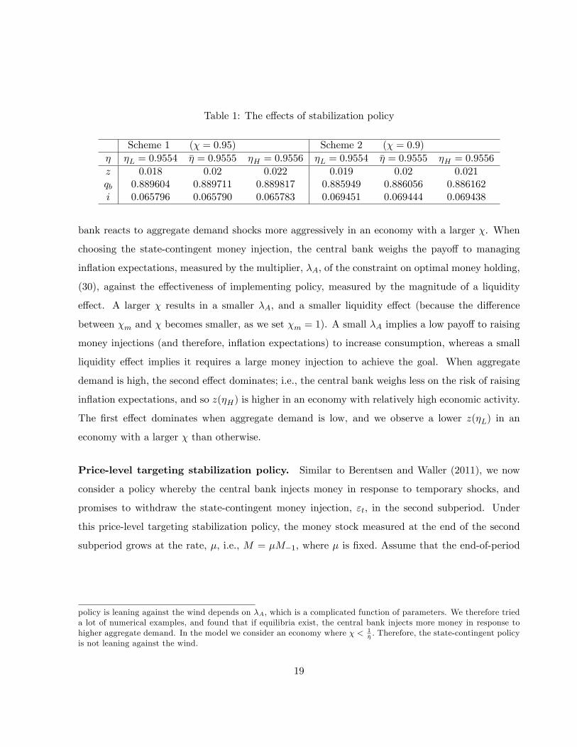
Table 1: The e¤ects of stabilization policy

Scheme 1 (� = 0:95) Scheme 2 (� = 0:9)

� �L = 0:9554 �� = 0:9555 �H = 0:9556 �L = 0:9554 �� = 0:9555 �H = 0:9556

z 0:018 0:02 0:022 0:019 0:02 0:021qb 0:889604 0:889711 0:889817 0:885949 0:886056 0:886162i 0:065796 0:065790 0:065783 0:069451 0:069444 0:069438

bank reacts to aggregate demand shocks more aggressively in an economy with a larger �. When

choosing the state-contingent money injection, the central bank weighs the payo¤ to managing

in�ation expectations, measured by the multiplier, �A; of the constraint on optimal money holding,

(30), against the e¤ectiveness of implementing policy, measured by the magnitude of a liquidity

e¤ect. A larger � results in a smaller �A; and a smaller liquidity e¤ect (because the di¤erence

between �m and � becomes smaller, as we set �m = 1). A small �A implies a low payo¤ to raising

money injections (and therefore, in�ation expectations) to increase consumption, whereas a small

liquidity e¤ect implies it requires a large money injection to achieve the goal. When aggregate

demand is high, the second e¤ect dominates; i.e., the central bank weighs less on the risk of raising

in�ation expectations, and so z(�H) is higher in an economy with relatively high economic activity.

The �rst e¤ect dominates when aggregate demand is low, and we observe a lower z(�L) in an

economy with a larger � than otherwise.

Price-level targeting stabilization policy. Similar to Berentsen and Waller (2011), we now

consider a policy whereby the central bank injects money in response to temporary shocks, and

promises to withdraw the state-contingent money injection, "t; in the second subperiod. Under

this price-level targeting stabilization policy, the money stock measured at the end of the second

subperiod grows at the rate, �; i.e., M = �M�1; where � is �xed. Assume that the end-of-period

policy is leaning against the wind depends on �A; which is a complicated function of parameters. We therefore trieda lot of numerical examples, and found that if equilibria exist, the central bank injects more money in response tohigher aggregate demand. In the model we consider an economy where � < 1

��: Therefore, the state-contingent policy

is not leaning against the wind.

19

real balances are state-independent, ��1M�1 = �M = &: The central bank�s problem becomes

maxx;qb

W = U(x)� x+Z �

�[�u(qb)� (1� �)c(

�

1� � qb)]g(�)d�;

s.t. �Z �

�

1 + �i

1 + �g(�)d� = 1: (32)

We consider the same example where c(q) = q and u(q) = e�(1� e�q): Thus, one can solve for

i =1 + �� ���

: (33)

Compared with the state-dependent interest rate shown in (31), (33) shows perfect smoothing of

interest rates. The perfect interest rate smoothing is due to the functional forms considered in this

example. From the binding budget constraint, (21), we solve for

z(�) =�qb(�)(1 + �)� ���1M�1

��1M�1(34)

Using i = � � qb(�) and the fact the interest rates are state-independent, qb is higher when the

economy is hit by a larger �: A higher qb is supported by a higher money injection z(�); as can

be seen from (34). Under the price-targeting stabilization policy, the central bank always increases

the state-contingent money injection in response to higher aggregate demand.

The price-level targeting policy results in smaller �uctuations in consumption than the state-

contingent policy (see Appendix C). Moreover, the two policy regimes feature di¤erent management

of expectations, which is re�ected in the di¤erence between the constraints in the planner�s prob-

lems, (30) and (32). The central bank controls long-run in�ation expectations via the price-level

targeting policy, whereas when it lacks the ability to withdraw the state-contingent money injec-

tions, it must at least commit itself to a short-run expected in�ation, as shown in the constraint,

(30).

If the central bank cannot promise to withdraw state-contingent money injections, the liquidity

e¤ect does not exist when � = �m = 1: Notice that if � = �m = 1; the binding cash constraint

becomes qb =��1M�1

� ; and consumption is independent of state-contingent money injections. To

summarize, when banks hold liquidity bu¤ers and the central bank cannot commit itself to unrav-

eling state-contingent money injections, the existence of a liquidity e¤ect, and thus the success of

20

stabilization policy, rely on unexpected money injections being more liquid than the initial money

stock.

5.2 Random deposit withdrawals

So far we have assumed that banks hold 1�� fraction of deposits as reserves, where � is an exogenous

parameter. In this subsection we consider random deposit withdrawals to motivate banks�holding

reserves. The environment is the same as in the basic model except that some depositors face a

liquidity shock and withdraw deposits to �nance consumption. Banks thus need to hold reserves

to meet unanticipated withdrawals.

Liquidity shocks and deposit withdrawals. In the beginning of the �rst subperiod, an agent

receives a preference shock. With probability �c an agent can consume but cannot produce (called

the buyer); with probability �p the agent can produce but cannot consume (called the seller); with

probability �n he can neither consume nor produce (called the non-trader), where �c+ �p+ �n = 1.

We consider the following timing sequence. Money injections take place after the realization of

preference shocks. Then sellers and non-traders make deposits, banks make the decision of holding

reserves and extending loans. Banks close after taking deposits and making loans. After banks close,

non-traders receive a liquidity shock: with probability �nc a non-trader wants to consume (called

the late consumer), and with probability 1 � �nc he does not want to consume. Late consumers

can withdraw deposits from automatic teller machines to �nance consumption.

The probability, �nc; is a random variable. For the purpose of illustration, we assume that

�nc follows a discrete uniform distribution. In particular, �nc takes the value from the set, Snc =

f�1nc; �2nc; :::; �kncg; where 0 � �inc < �jnc � 1 if i < j; with an equal probability; that is, Pr(�nc =

�inc) =1k ; i = 1; 2; : : : ; k; where k � 2: We call shocks to �nc the liquidity shock, which arrives

in the following way. The Nature draws from the set, Snc; to determine the realized value of �nc;

denoted as �jnc: Then, a non-trader receives the liquidity shock that he wishes to consume with

probability �jnc; or does not wish to consume with probability 1 � �jnc: The liquidity shock is an

aggregate shock, since it implies that, by the law of large number, there is a proportion, �jnc; of

non-traders become late consumers. Given that the Nature has drawn �jnc; whether a non-trader

21

wishes to consumer is an idiosyncratic shock.

Because banks make the decision to hold reserves before the realization of liquidity shocks, and

there are no alternatives to obtain reserves in the interim period, they will hold reserves to meet

the demand for the largest amount of withdrawals from late consumers; i.e., banks hold �n�knc (per

capita) fraction of deposits as reserves.21 Banks do not pay interest on deposits withdrawn by late

consumers, because deposits and withdrawals are made within the same subperiod. It is clear now

why non-traders would make deposits: they can withdraw money if they wish to consume, and can

earn interest payments otherwise.

To focus our attention on motivating banks�holding reserves by random withdrawals, in the

current model we do not consider the case where non-traders make deposits as well as borrow

from banks, due to, e.g., spatial frictions.22 Moreover, we assume that banks do not take deposits

after make loans. Therefore, it is not possible that non-traders borrow without making deposits,

and deposit all money after they learn that they do not want to consume. Notice that restricting

the opportunity for non-traders to borrow can distort allocations. In Appendix D we relax these

restrictions and derive the condition for non-traders to take loans.

Trade and bank operations in the �rst subperiod. The liquidity shock results in aggregate

uncertainty, so we denote variables that depend on the state �jnc with a superscript j; where j =

1; 2; : : : ; k: For examples, pj denotes the price in the �rst subperiod, and qjl the consumption by a

late consumer. Let dn denote a non-trader�s deposits.23

In the goods market a seller�s problem and a buyer�s problem are similar to those in Section

4. A non-trader maximizes his expected utility by choosing the deposits, dn; and the quantity

consumed if he becomes a late consumer, qjl :

21 In reality banks facing unexpected deposit withdrawals can resort to the interbank loan market, the centralbank�s discount window, or calling back loans. We do not consider those possibilities in this paper, and so banks needto meet the unexpected withdrawals with their own reserves. Even given those possible ways of obtaining reserves,weighing the cost of the alternative resorts against that of holding reserves, banks may still keep some excess reserves.

22One type of such spacial frictions can work as follows. Suppose there is a location shock which is perfectlycorrelated to the preference shock. The shock locates sellers and non-traders to banks�deposits service units, whilelocate buyers in units of lending money. Banks�deposits and lending service units are spacially separated, and agentsare time constrained to visit more than one service unit.

23As in the basic model, the price and quantities consumed and produced should also depend on the moneyinjection, z; but we suppress the dependence of those variables on z: Because deposits and loans are made before theliquidity shock is realized, dn and b do not depend on the state, �jnc, neither do interest rates.

22

maxqjl ;dn�0

1

k

kXj=1

�jnc[u(qjl ) +W (m� p

jqjl ; 0)] + (1� �jnc)W (m� dn; dn)

s.t. pjqjl � m;

dn � m:

With probability �jnc a non-trader becomes a late consumer and uses money holdings left after

deposits, m�dn; plus deposits withdrawn, dn; to �nance consumption, pjqjl , while with probability

1� �jnc a non-trader does not want to consume, and he enters the second subperiod holding m�dnunits of money and dn deposits. The �rst order condition implies that non-traders deposit all

money holdings, and dn = m: Moreover, u0(qjl ) = c0(qjs) when the cash constraint does not bind;

otherwise, the late consumer spends all his money and

qjl =m

pj: (35)

The expected utility of an agent entering the �rst subperiod of period t with money holdings,

m; is

V (m) =1

k

kXj=1

Z�c[u(q

jb) +W (m+ b� p

jqjb ; b)] + �n

��jnc[u(q

jl ) +W (m� pjq

jl ; 0)]

+(1� �jnc)W (m� dn; dn)

�+ �p[�c(qjs) +W (m� d+ pjqjs; d)]f(z)dz

The marginal value of money is

Vm(m) =1

k

kXj=1

Z (�cu0(qjb)

pj+ �n[�

jnc

u0(qjl )

pj+ (1� �jnc)�(1 + id)] + �p�(1 + id)

)f(z)dz: (36)

The bene�ts of holding an additional unit of money to the �rst subperiod include expected gains

from spending the money on goods as a buyer or as a late consumer, and the deposits interest as a

seller or as a non-trader who does not want to consume.24 Using (3) lagged one period to eliminate

Vm(m) from (36), an agent�s optimal money holdings satisfy

�1

k

kXj=1

Z (�cu0(qjb)pj

+ �n[�jncu0(qjl )pj

+ (1� �jnc)�(1 + id)]+�p�(1 + id)

)f(z)dz � ��1;�= �if m > 0: (37)

24Because of the stationary condition, �t�1Mt�1 = �tMt; the value of money in the second subperiod of t; �t; isindependent of �jnc:

23

Sellers, buyers, and late consumers trade in the goods market in the �rst subperiod. In a

symmetric equilibrium, the market-clearing conditions in state j for goods, loans, and money are

�pqjs = �cq

jb + �n�

jncq

jl ; for all j; (38)

�cb = [�p + �n(1� �knc)]d+ �m� ; (39)

and m = M�1; respectively. In the loan market clearing condition, (39), given that banks hold

�n�knc fraction of deposits as reserves, the per capita funds available for banks to lend out include

�p + �n(1 � �knc) fraction of deposits, and �m fraction of injected money, while per capita loans

demanded is �cb: Though we still let �m be a parameter, note that in this economy banks may well

use up all injected money to extend loans.

The zero marginal pro�t condition, which ensures that a bank cannot become in�nitely prof-

itable by attracting in�nitely large amount of funds is

�p + �n(1� �knc)�p + �n(1� �nc)

i = id;

where �nc = 1k

Pkj=1 �

jnc: In the basic model the zero marginal pro�t condition is �i = id; where

� is a parameter. Here we have derived the fraction of deposits that banks lend out when facing

random deposit withdrawals.

The liquidity e¤ect under random deposit withdrawals. We use a similar approach as in

Section 4 to derive conditions for the existence of a liquidity e¤ect (see Appendix D for derivation).

We consider equilibria where the cash constraint binds for buyers and late consumers in all states.

Let qjA denote the aggregate demand in state j: Then

qjA = �cqjb + �n�

jncq

jl =

(�l + �mz + �n�jnc)��1M�1

c0(qjs)(1 + z); (40)

where

�l = �c + �p + �n(1� �knc) = 1� �n�knc:

Note that �l is the fraction of the initial money stock, M�1; that can be used to �nance spending.

(We drop the superscript j below where there is no confusion.) Taking the derivative of qA with

24

respect to z we obtain

@qA@z

=��1M�1(�m � �l � �n�nc)(1 + z)2[c0( qA�p ) +

qA�pc00( qA�p )]

8<:> >= 0 i¤ �m = �l + �n�nc:< <

(41)

The existence of a liquidity e¤ect (@qA@z > 0) depends on �m > �l + �n�nc: If �nc = �knc, we have

�l + �n�knc = 1; and even when banks lend out all money injected (�m = 1); there is no liquidity

e¤ect. Because �nc = �knc occurs with probability1k , a liquidity e¤ect is more likely to exist when

k is larger.

When a liquidity e¤ect exists, monetary policy has an (interim) redistribution e¤ect between

buyers and late consumers. Note that qb is increased by z if �m > �l; that is, unanticipated

money injections bene�t buyers if the loanable funds e¤ect dominates the Fisher e¤ect. However,

ql is decreased by z because the loanable funds e¤ect is absent for late consumers and only the

Fisher e¤ect applies. Consequently, money injections hurt late consumers. When a liquidity e¤ect

exists, therefore, unanticipated money injections redistribute consumption from late consumers to

buyers. Moreover, for aggregate demand to increase by money injections, the increase in the buyer�s

consumption must outweigh the decrease in the late consumer�s consumption.

Using the stationary condition, ��1M�1 = �M; and the total funds available per buyer to

�nance consumption in the �rst subperiod, m+ b = (�l+�mz)�c

M�1; we have the following version of

the equation of exchange:

pqA =(�l + �mz + �n�nc)

(1 + z)M; (42)

where the left of (42) is the aggregate demand for goods, and in the right, (�l+�mz+�n�nc)(1+z) is the

velocity of money. Compared to the velocity in the basic model, �+�mz(1+z) ; in this environment the

velocity is volatile due to the uncertainty from the consumption of late consumers. The larger

the probability of being a late consumer, the higher the velocity. If there exists a liquidity e¤ect

(�m > �l + �n�nc), an unexpected money injection raises velocity and total liquidity, which leads

to higher output and prices.

25

6 Conclusion

The current paper features �exible prices and frictions, which give rise to the roles of money and

�nancial intermediation. A liquidity e¤ect exists if and only if the fraction of money injections used

to �nance spending is larger than that of the initial money stock. If banks hold no liquidity bu¤ers,

the liquidity e¤ect is eliminated. We extend the model by incorporating aggregate demand shocks

to study optimal stabilization policy, and the need for liquidity management due to random deposit

withdrawals to motivate banks�holding reserves. In contrast to Berentsen and Waller (2011), failure

to unravel state-contingent money injections in our model does not make the stabilization policy

neutral. The price-level targeting policy, however, results in smaller �uctuations in consumption

than the state-contingent policy. Finally, in an economy where banks hold liquidity bu¤ers, when

the central bank cannot commit itself to a price-level path, the existence of a liquidity e¤ect and

the success of stabilization policy rely on unexpected money injections being more liquid than the

initial money stock.

26

References

Basel Committee on Banking Supervision (2000). �Basel III: International framework for liq-

uidity risk measurement, standards and monitoring.�Available at http://www.bis.org/publ/

bcbs188.pdf.

Bencivenga, V.R. and G. Camera (2011). �Banking in a Matching Model of Money and Capital,�

Journal of Money, Credit and Banking 43, 449-476.

Berentsen, A., G. Camera and C. Waller (2007). �Money, Credit and Banking,� Journal of

Economic Theory 135, 171-195.

Berentsen, A. and C. Waller (2011). �Price Level Targeting and Stabilization Policy,�Journal of

Money, Credit and Banking 43, 559-580.

Christiano, L. (1991). �Modelling the Liquidity E¤ect of a Monetary Shock,� Federal Reserve

Bank of Minneapolis Quarterly Review, 3-34.

Cochrane, J.H. (2014).�Monetary policy with Interest on Reserves,�Journal of Economic Dynam-

ics & Control 49, 74-108.

Diamond, D. and P. Dybvig (1983). �Bank Runs, Deposit Insurance and Liquidity,� Journal of

Political Economy 91, 401-19.

Freedman, P. and R. Click (2006). �Banks that don�t lend? Unlocking credit to spur growth in

developing countries,�Development Policy Review 24, 279-302.

Fuerst, T. (1992). �Liquidity, Loanable funds and Real activity,�Journal of Monetary Economics

29, 3-24.

Fuerst, T. (1994). �Monetary Policy and Financial Intermediation,� Journal of Money, Credit

and Banking 26, 362-376.

Grossman S. and L. Weiss (1983). �A Transactions-Based Model of the Monetary Transmission

Mechanism,�American Economic Review 73, 871-80.

27

Kashyap, A., R. Rajan and J. Stein (2002). �Banks as Liquidity Providers: An Explanation for

the Coexistence of Lending and Deposit-Taking,�Journal of Finance LVII, 33-73.

Lagos, R. and R. Wright (2005). �A Uni�ed Framework for Monetary Theory and Policy Analysis,�

Journal of Political Economy 113, 463-84.

Li, Y., and Y. Li (2013). �Liquidity and asset prices: A new monetarist approach,�Journal of

Monetary Economics 60, 426-438.

Lucas, R. (1990). �Liquidity and the Interest Rates,�Journal of Economic Theory 50, 237-264.

Ratnovski, L. (2009). �Bank liquidity regulation and the lender of last resort,�Journal of Financial

Intermediation 18, 541-558.

Rotemberg, J. (1984). �A Monetary Equilibrium Model with Transactions Costs,� Journal of

Political Economy 92, 40-58.

Williamson, S. (2004).�Limited Participation, Private Money, and Credit in a Spatial Model of

Money,�Economic Theory 24, 857-876.

Williamson, S. (2006). �Search, Limited Participation, and Monetary Policy,�International Eco-

nomic Review 47, 107-128.

28

A Solving the bank�s problem

Banks are perfectly competitive with free entry, they take as given the loan rate and the deposit rate.

There is no strategic interaction among banks or between banks and agents, and no bargaining over

the terms of the loan contract. A pro�t maximizing bank turns out to solve the following problem

per borrower:

maxb(i� id

�)b

s.t. u(qb) +W (m; b; d) � �;

where � is the reservation value of the borrower, which is the surplus from obtaining loans at

another bank. The �rst order condition to the bank�s problem is

i� id�+ ��[u

0(qb)dqbdb+Wb] = 0; (43)

where �� is the Lagrangian multiplier on the borrower�s participation constraint. For i � id� > 0,

the bank would like to make the largest loan possible to borrowers. Therefore, this implies a zero

marginal pro�t condition,

�i = id:

and the bank would choose a loan amount such that �� > 0.

From (8) and the buyer�s budget constraint, dqbdb =�

c0(qs): Using Wb = ��(1 + i); from (43) we

haveu0(qb)

c0(qs)= 1 + i:

29

B Financial intermediation and the Friedman rule

We now show that the Friedman rule achieves the �rst-best allocation in our model. Our discussion

on the Friedman rule is similar to that in Berentsen, Camera, and Waller (2005), who consider the

real e¤ect of monetary injections without the banking system. Consider �rst the benchmark case

where banks lend out all deposits and money injections, and so the loan rate equals the deposit

rate. In a monetary economy, from (8) and (12), (14) becomes

�E�1[�(1 + id)] = ��1 (44)

We de�ne the expected real return on money as 11+ ̂ ; i.e., E�1

���1

� 11+ ̂ . To implement the

Friedman rule in this economy, the central bank must set the expected return on money equal to

the real interest rate; i.e., 11+ ̂ =

1� ; which implies id = 0 by (44). Hence, u

0(qb) = c0(qs) by (12),

and Friedman rule achieves the �rst-best allocation. The Friedman rule ensures that agents can

perfectly insure themselves against monetary shocks because holding currency has zero costs.

The Friedman rule, however, may require a positive money growth rate in the environment with

unexpected money injections. Consider an example in which the money growth rate, z; is a random

variable such that

z =

�zh = �(1 + �) with probability 1

2 ;z` = �(1� �) with probability 1

2 ;

where �; � > 0: The stationary condition implies that 1 + zh =��1�h

and 1 + z` =��1�`. The average

in�ation is � = Ez> 0; and the average return on money is

1

1 + ̂� E�1

�

��1=

1

(1 + �)(1� �2) :

One can see that � > ̂ and if � >p1� �, the money growth rate in Friedman rule is positive.

In a monetary economy where banks hold liquidity bu¤ers the Friedman rule also achieves the

e¢ cient allocation. From (8) and �i = id; equation (14) becomes

�E�1�[�(1 + i) + (1� �)(1 + id)] = ��1: (45)

From (45) we see that, under the policy that sets 1+ ̂ = �; u0(qb) = c0(qs) as id and i approach to

0. The Friedman rule achieves the e¢ cient allocation.

30

Reference

Berentsen A., G. Camera, and C. Waller (2005). �The Distribution of Money Balances and the

Non-neutrality of Money,�International Economic Review 46, 465-480.

31

C Deriving optimal money injections under demand shocks

The central bank�s problem is:

maxx;qb

W = U(x)� x+Z �

�[�u(qb)� (1� �)c(

�

1� � qb)]g(�)d�;

s.t. �Z �

�

(1 + �i)(��1M�1 � �qb)��1M�1(1� �)

g(�)d� = 1:

Because 1 + i = u0(qb)c0(qs)

= e��qb , we use the approximation, log(1 + y) ' y; to get i(�) ' � � qb(�).

Let �A be the multiplier of the constraint (30). The �rst order conditions are U 0(x) = 1, andZ �

�[�e��qb � �]g(�)d� � ��A

��1M�1(1� �)

Z �

�f�(��1M�1 � �qb) + [1 + �(� � qb)�gg(�)d� = 0;

where �A is the multiplier of the constraint, (30). Simplifying the above equation and use the

approximation i � � � qb, we obtain i(�) de�ned in (31). Assuming a particular distribution of

�; and substituting i(�) from (31) into the constraint (30), one could obtain �A as a function of

parameters such as �, �, �, ��1M�1 and �.

Assume that � follows a Bernoulli distribution such that � takes a value from the set f�L; ��; �Hg

with an equal probability, 13 ; where �� = (�H + �L)=2. This implies that i = iH = i(�H) with

probability 13 , i = i�� = i(��) with probability

13 ; and i = iL = i(�L) with probability

13 . Rewrite i(�)

as:

i(�) =1 + �(

��1M�1� � �)

(1��)��1M�1��A

� 2�: (46)

We can solve for the real balance, ��1M�1; from the long-run equilibrium, in which � = �� and

z = �: Therefore, in the long-run equilibrium, 1 + �i�� =(1+�)� , qb =

��1M�1(�+�)�(1+�) ; and i�� = �� � qb:

We obtain

��1M�1 =�(1 + �)

�+ �(�� � 1 + �� �

��); (47)

i�� =1 + �� ���

: (48)

Note that i�� � 0 if and only if � � �� 1: Denote �0 = �� 1: Let n and d denote the numerator

32

and denominator, respectively, of i(��) in (46); that is,

n = 1 + �(��1M�1

�� ��)

d =(1� �)��1M�1

��A� 2�

Using (47) we obtain

n =�(1� �)�+ �

�� + 1� � 1 + ��+ �

1 + �� ���

:

The numerator of i(��); n > 0; if and only if �1 < � < �2; where �1 = �1+��p� [� � (1� �)(1� ���)]

and �2 = �1 + � +p� [� � (1� �)(1� ���)]: The real balance, ��1M�1; shown in (47), is strictly

positive i¤ � < �3; where �3 = �1+�+����: Note that �1 < �0; and �3 < �2 i¤ � < 1�� : Therefore,

when � < 1�� ; the condition, � 2 [�0; �3]; implies that n > 0; and that to get i(��) � 0 we need the

denominator of i(��) from (46) to be positive.

We now show that under certain condition, the central bank would not choose a policy that

is leaning against the wind (i.e., a policy that leads to z(�H) < z(�L); and so iH > iL): Di¤eren-

tiating i(�) from (46) with respect to �; one obtain @i@� =

�1[(1��)��1M�1=��A�2�] : Then,

@i@� > 0 i¤

(1��)��1M�1��A

� 2� < 0; i.e., the denominator of i(��); d < 0: In order for i(��) � 0; we need n � 0;

which implies that either � � �1 or � � �2: Because �1 < �0; we thus need � � �2 to get n � 0:

But if � < 1�� ; under the condition � � �2; the real balance is negative, and the equilibrium does

not exist. Therefore, if � < 1�� ; the central bank injects more money in response to higher aggregate

demand. In the model we consider an economy where � < 1�� :25

Comparing �uctuations of consumption under the state-contingent stabilization policy

and the price-level targeting stabilization policy. Here we use the variance of consumption

to measure �uctuations. Let qjwb and qjob (i

jw and i

jo) denote the buyer�s consumption (interest rates)

under the policy with and without withdrawal of the state-contingent money injection, respectively,

25 If � > 1��; then �2 < �3; it�s possible to �nd a � 2 (�2; �3) under which n < 0: If in this case we can �nd

d < 0; and so the interest rate and real balance are positive, we cannot preclude the possibility that the centralbanks chooses a policy that is leaning against the wind. Since d depends on �A; which is a complicated functionof parameters, we cannot obtain explicit conditions for d > 0: From a lot of numerical examples we found thatif � > 1

��and � 2 (�2; �3); equilibria do not exist, but when � < �2; the central bank injects more money in response

to higher aggregate demand.

33

where j = H;L represents that the state is � = �H or � = �L. Let �qwb and �qob (�2w and �

2o) denote

the average (variance) of consumption under policy with and without withdrawal of the state-

contingent money injection, respectively, when � = �� = �H+�L2 :

Under the price-level targeting stabilization policy, from (33), iw =1+����� . Then, �qwb = ��� iw:

Under the state-contingent stabilization policy whereby the central bank does not withdraw the

state-contingent money injection, �qob = �� � iHo +iLo

2 : Let ! = iHo �iLo2 : Then,

�2o � �2w = [(qHob � �qob)2 + (qLob � �qob)2]� [(qHwb � �qwb)2 + (qLwb � �qwb)2]

= [(�H � �� � !)2 + (�L � �� + !)2]� [(�H � ��)2 + (�L � ��)2]

= 2!(! � �H + �L):

Under the state-contingent policy, iH < iL: Therefore, ! < 0; and �2o > �2w; the price-level targeting

policy results in smaller �uctuations than the state-contingent policy.

34

D Random deposit withdrawals

Solving the bank�s problem. The representative bank�s expected pro�t is

�cib�1

k

kXj=1

��p + �n(1� �jnc)

�did;

where b and d satisfy the market-clearing condition for loans, (39). Substituting d from (39) into

the bank�s expected pro�t, we obtain that a bank solves the following problem per borrower:

maxb(i� id

~�)b

s.t.1

k

kXj=1

hu(qjb) +W (m; b; d)

i� �c;

where �c is the reservation value of the borrower, which is the surplus from obtaining loans at

another bank, and ~� = �p+�n(1��knc)1k

Pkj=1[�p+�n(1��

jnc)]. The �rst order condition to the bank�s problem is

i� id~�+ ��c

1

k

kXj=1

[u0(qjb)dqjbdb

+Wb] = 0; (49)

where ��c is the Lagrangian multiplier on the borrower�s participation constraint. For i� id~� > 0,

the bank would like to make the largest loan possible to borrowers. Therefore, this implies a zero

marginal pro�t condition,

~�i = id:

and the bank would choose a loan amount such that ��c > 0.

From (8) and the buyer�s budget constraint, dqjbdb =

�

c0(qjs): Using Wb = ��(1 + i); from (49) we

have1

k

kXj=1

u0(qjb)

c0(qjs)= 1 + i:

We now consider the buyer�s problem.

maxqjb ;b�0

1

k

kXj=1

[u(qjb) +W (m+ b� pjqjb ; b)]

s.t. pjqjb � m+ b;

The �rst order condition with respect to b is 1k

kPj=1

u0(qjb)

c0(qjs)= 1 + i: A buyer borrows to the point at

which the expected bene�t of �nancing consumption equals the borrowing cost.

35

Deriving the condition for a liquidity e¤ect. We use a similar approach as in Section 4 to

derive conditions for the existence of a liquidity e¤ect. From the loan-market-clearing condition,

(39), we have

b =[�p + �n(1� �knc)]d+ �m�

�c: (50)

Substituting d = m; � = zM�1; and m = M�1 into (50), we obtain the total funds available per

buyer to �nance consumption in the �rst subperiod:

m+ b =(�l + �mz)

�cM�1; (51)

where

�l = �c + �p + �n(1� �knc) = 1� �n�knc:

We consider an equilibrium where the cash constraint binds in all states, qjb =m+bpj, from which we

derive

qjbc0(qjs) =

(�l + �mz)��1M�1�c(1 + z)

; (52)

by using (8), (51), and 1 + z =��1� : A similar condition for the late consumer is

qjl c0(qjs) =

��1M�1(1 + z)

: (53)

The aggregate demand, qjA; is thus

qjA = �cqjb + �n�

jncq

jl =

(�l + �mz + �n�jnc)��1M�1

c0(qjs)(1 + z):

From (53), qjl is decreased by the money injection, z; whereas from (52), qjb is increased by z if

�m > �l: Taking the derivative of qjA with respect to z; we obtain condition (41).

Relaxing the restrictions so that non-traders may borrow. We �rst consider an environ-

ment with no spatial frictions, where non-traders can make deposits and take loans. Let bn and dn

denote the loan amount and deposits made by a non-trader, respectively, before the liquidity shock

36

is realized. A non-trader�s problem is

maxqjl ;bn;dn�0

1

k

kXj=1

�jnc[u(qjl ) +W (m+ bn � p

jqjl ; bn; 0)] + (1� �jnc)W (m+ bn � dn; bn; dn) (54)

s.t. pjqjl � dn + bn;

dn � m:

The �rst term in (54) shows that with probability �jnc a non-trader becomes a late consumer and

uses money holdings left after deposits, m�dn; plus deposits withdrawn, dn; and loan, bn; to �nance

consumption, pjqjl . The second term in (54) implies that with probability 1��jnc a non-trader does

not want to consume, and he enters the second subperiod holding m� dn + bn units of money, bndebt, and dn deposits. The �rst order condition with respect to bn is

1

k

kXj=1

�jncu0(qjl )

c0(qjs)� 1 + i; �= �if bn > 0: (55)

Condition (55) implies that when the expected net bene�t of borrowing to �nancing consumption

o¤sets the loan interests, a non-trader has incentives borrow. Given the loan rate, (55) is less likely

to hold at equality if �jnc is smaller. That is, when the future opportunity for consumption is slim

non-traders are less likely to incur the borrowing cost to take out loans.

Next, consider an environment where banks take deposits after the liquidity shock is realized.

Suppose a non-trader borrow bn before the liquidity shock is realized. We consider the situation

where once a non-trader learns that he does not want to consume, he deposits the money initially

held and the borrowed money (this is innocuous because, if we assume there is a cost of withdrawing

deposits, � > 0; non-traders would not make deposits before the liquidity shock is realized.) Let djn

denote deposits made by a non-trader after the liquidity shock is realized, when the state is �jnc. A

non-trader solves the following problem

maxqjn;bn;d

jn�0

1

k

kXj=1

�jnc[u(qjl ) +W (m+ bn � p

jqjl ; bn; 0)] + (1� �jnc)W (m+ bn � dn; bn; djn)

s.t. pjqjl � m+ bn;

djn � m+ bn:

37

With probability �jnc a non-trader is a late consumer, and he spends his money holding and

borrowed money, m+ bn; to �nance consumption, and with probability 1��jnc; he does not want to

consume, and deposits djn in the bank. Note that djn = m+ bn; for all j; because making deposits

would earn interests. The �rst order condition is

1

k

kXj=1

"�jncu0(qjl )

c0(qjs)+ (1� �jnc)(1 + id)

#� (1 + i); �= �if bn > 0: (56)

When (56) holds with equality, a non-trader borrows to the point at which the borrowing cost equals

the expected bene�t of �nancing consumption plus the expected bene�t of depositing money if he

does not want to consume. Because here banks are ready to accept deposits after the liquidity shock

is realized, non-traders do not need to make deposits before the realization of liquidity shocks, and

so there is no withdrawal uncertainty facing banks. This is di¤erent from our motivation to justify

banks�holding reserves to insure against random deposit withdrawals.

38