Code of Practice

CODE OF PRACTICE 2007 CODE OF PRACTICE 2007 CODE OF PRACTICE 2007 CODE OF PRACTICE 2007 CODE OF PRACTICE 2007 CODE OF PRACTICE 2007 CODE OF PRACTICE 2007 CODE OF PRACTICE 2007 CODE OF PRACTICE 2007 CODE OF PRACTICE 2007 CODE OF PRACTICE 2007 CODE OF PRACTICE 2007 CODE OF PRACTICE 2007 CODE OF PRACTICE 2007 CODE OF PRACTICE 2007 CODE OF PRACTICE 2007 CODE OF PRACTICE 2007 CODE OF PRACTICE 2007 CODE OF PRACTICE 2007 CODE OF PRACTICE 2007 CODE OF PRACTICE 2007 CODE OF PRACTICE 2007 CODE OF PRACTICE 2007 CODE OF PRACTICE 2007 CODE OF PRACTICE 2007 CODE OF PRACTICE 2007 CODE OF PRACTICE 2007 CODE OF PRACTICE 2007 CODE OF PRACTICE 2007 CODE OF PRACTICE 2007 CODE OF PRACTICE 2007 CODE OF PRACTICE 2007 CODE OF PRACTICE 2007 CODE OF PRACTICE 2007 CODE OF PRACTICE 2007 CODE OF PRACTICE 2007 CODE OF PRACTICE 2007 CODE OF PRACTICE 2007 CODE OF PRACTICE 2007 CODE OF PRACTICE 2007 CODE OF PRACTICE 2007 CODE OF PRACTICE 2007 CODE OF PRACTICE 2007 CODE OF PRACTICE 2007 CODE OF PRACTICE 2007 CODE OF PRACTICE 2007 CODE OF PRACTICE 2007 CODE OF PRACTICE 2007 CODE OF PRACTICE 2007 CODE OF PRACTICE 2007 CODE OF PRACTICE 2007 CODE OF PRACTICE 2007 CODE OF PRACTICE 2007 CODE OF PRACTICE 2007 CODE OF PRACTICE 2007 CODE OF PRACTICE 2007 CODE OF PRACTICE 2007 CODE OF PRACTICE 2007 CODE OF PRACTICE 2007 CODE OF PRACTICE 2007 CODE OF PRACTICE 2007 CODE OF PRACTICE 2007 CODE OF PRACTICE 2007 CODE OF PRACTICE 2007 CODE OF PRACTICE 2007 CODE OF PRACTICE 2007 CODE OF PRACTICE 2007 CODE OF PRACTICE 2007 CODE OF PRACTICE 2007 CODE OF PRACTICE 2007 CODE OF PRACTICE 2007 CODE OF PRACTICE 2007 CODE OF PRACTICE 2007 CODE OF PRACTICE 2007 CODE OF PRACTICE 2007 CODE OF PRACTICE 2007 CODE OF PRACTICE 2007 CODE OF PRACTICE 2007 CODE OF PRACTICE 2007 CODE OF PRACTICE 2007 CODE OF PRACTICE 2007 CODE OF PRACTICE 2007 CODE OF PRACTICE 2007 CODE OF PRACTICE 2007 CODE OF PRACTICE 2007 CODE OF PRACTICE 2007 CODE OF PRACTICE 2007 CODE OF PRACTICE 2007 CODE OF PRACTICE 2007 CODE OF PRACTICE 2007 CODE OF PRACTICE 2007 CODE OF PRACTICE 2007 CODE OF PRACTICE 2007 CODE OF PRACTICE 2007 CODE OF PRACTICE 2007 CODE OF PRACTICE 2007 CODE OF PRACTICE 2007 CODE OF PRACTICE 2007 CODE OF PRACTICE 2007 CODE OF PRACTICE 2007 CODE OF PRACTICE 2007 CODE OF PRACTICE 2007 CODE OF PRACTICE 2007 CODE OF PRACTICE 2007 CODE OF PRACTICE 2007 CODE OF PRACTICE 2007 CODE OF PRACTICE 2007 CODE OF PRACTICE 2007 CODE OF PRACTICE 2007 CODE OF PRACTICE 2007 CODE OF PRACTICE 2007 CODE OF PRACTICE 2007 CODE OF PRACTICE 2007 CODE OF PRACTICE 2007 CODE OF PRACTICE 2007 CODE OF PRACTICE 2007 CODE OF PRACTICE 2007 CODE OF PRACTICE 2007 CODE OF PRACTICE 2007 CODE OF PRACTICE 2007 CODE OF PRACTICE 2007 CODE OF PRACTICE 2007 CODE OF PRACTICE 2007 CODE OF PRACTICE 2007 CODE OF PRACTICE 2007 CODE OF PRACTICE 2007 CODE OF PRACTICE 2007 CODE OF PRACTICE 2007 CODE OF PRACTICE 2007 CODE OF PRACTICE 2007 CODE OF PRACTICE 2007 CODE OF PRACTICE 2007 CODE OF PRACTICE 2007 CODE OF PRACTICE 2007 CODE OF PRACTICE 2007 CODE OF PRACTICE 2007 CODE OF PRACTICE 2007 CODE OF PRACTICE 2007 CODE OF PRACTICE 2007 CODE OF PRACTICE 2007 CODE OF PRACTICE 2007 CODE OF PRACTICE 2007 CODE OF PRACTICE 2007 CODE OF PRACTICE 2007 CODE OF PRACTICE 2007 CODE OF PRACTICE 2007 CODE OF PRACTICE 2007 CODE OF PRACTICE 2007 CODE OF PRACTICE 2007 CODE OF PRACTICE 2007 CODE OF PRACTICE 2007 CODE OF PRACTICE 2007 CODE OF PRACTICE 2007 CODE OF PRACTICE 2007 CODE OF PRACTICE 2007 CODE OF PRACTICE 2007 CODE OF PRACTICE 2007 CODE OF PRACTICE 2007 CODE OF PRACTICE 2007 CODE OF PRACTICE 2007 CODE OF PRACTICE 2007 CODE OF PRACTICE 2007 CODE OF PRACTICE 2007 CODE OF PRACTICE 2007 CODE OF PRACTICE 2007 CODE OF PRACTICE 2007 CODE OF PRACTICE 2007 CODE OF PRACTICE 2007 CODE OF PRACTICE 2007 CODE OF PRACTICE 2007 CODE OF PRACTICE 2007 CODE OF PRACTICE 2007 CODE OF PRACTICE 2007 CODE OF PRACTICE 2007 CODE OF PRACTICE 2007 CODE OF PRACTICE 2007 CODE OF PRACTICE 2007 CODE OF PRACTICE 2007 CODE OF PRACTICE 2007 CODE OF PRACTICE 2007 CODE OF PRACTICE 2007 CODE OF PRACTICE 2007 CODE OF PRACTICE 2007 CODE OF PRACTICE 2007 CODE OF PRACTICE 2007 CODE OF PRACTICE 2007 CODE OF PRACTICE 2007 CODE OF PRACTICE 2007 CODE OF PRACTICE 2007 CODE OF PRACTICE 2007 CODE OF PRACTICE 2007 CODE OF PRACTICE 2007 CODE OF PRACTICE 2007 CODE OF PRACTICE 2007 CODE OF PRACTICE 2007 CODE OF PRACTICE 2007 CODE OF PRACTICE 2007 CODE OF PRACTICE 2007 CODE OF PRACTICE 2007 CODE OF PRACTICE 2007 CODE OF PRACTICE 2007 CODE OF PRACTICE 2007 CODE OF PRACTICE 2007 CODE OF PRACTICE 2007 CODE OF PRACTICE 2007 CODE OF PRACTICE 2007 CODE OF PRACTICE 2007 CODE OF PRACTICE 2007 CODE OF PRACTICE 2007 CODE OF PRACTICE 2007 CODE OF PRACTICE 2007 CODE OF PRACTICE 2007 CODE OF PRACTICE 2007 CODE OF PRACTICE 2007 CODE OF PRACTICE 2007 CODE OF PRACTICE 2007 CODE OF PRACTICE 2007 CODE OF PRACTICE 2007 CODE OF PRACTICE 2007 CODE OF PRACTICE 2007 CODE OF PRACTICE 2007 CODE OF PRACTICE 2007 CODE OF PRACTICE 2007 CODE OF PRACTICE 2007 CODE OF PRACTICE 2007 CODE OF PRACTICE 2007 CODE OF PRACTICE 2007 CODE OF PRACTICE 2007 CODE OF PRACTICE 2007 CODE OF PRACTICE 2007 CODE OF PRACTICE 2007 CODE OF PRACTICE 2007 CODE OF PRACTICE 2007 CODE OF PRACTICE 2007 CODE OF PRACTICE 2007 CODE OF PRACTICE 2007 CODE OF PRACTICE 2007 CODE OF PRACTICE 2007 CODE OF PRACTICE 2007 CODE OF PRACTICE 2007 CODE OF PRACTICE 2007 CODE OF PRACTICE 2007 CODE OF PRACTICE 2007 CODE OF PRACTICE 2007 CODE OF PRACTICE 2007 CODE OF PRACTICE 2007 CODE OF PRACTICE 2007 CODE OF PRACTICE 2007 CODE OF PRACTICE 2007 CODE OF PRACTICE 2007 CODE OF PRACTICE 2007 CODE OF PRACTICE 2007 CODE OF PRACTICE 2007 CODE OF PRACTICE 2007 CODE OF PRACTICE 2007 CODE OF PRACTICE 2007 CODE OF PRACTICE 2007 CODE OF PRACTICE 2007 CODE OF PRACTICE 2007 CODE OF PRACTICE 2007 CODE OF PRACTICE 2007 CODE OF PRACTICE 2007 CODE OF PRACTICE 2007 CODE OF PRACTICE 2007 CODE OF PRACTICE 2007 CODE OF PRACTICE 2007 CODE OF PRACTICE 2007 CODE OF PRACTICE 2007 CODE OF PRACTICE 2007 CODE OF PRACTICE 2007

Staff Working Paper No. 782The impact of corporate QE on liquidity: evidence from the UKLena Boneva, David Elliott, Iryna Kaminska, Oliver Linton, Nick McLaren and Ben Morley

July 2020This is an updated version of the Staff Working Paper originally published on 1 March 2019

Staff Working Papers describe research in progress by the author(s) and are published to elicit comments and to further debate. Any views expressed are solely those of the author(s) and so cannot be taken to represent those of the Bank of England or to state Bank of England policy. This paper should therefore not be reported as representing the views of the Bank of England or members of the Monetary Policy Committee, Financial Policy Committee or Prudential Regulation Committee.

Staff Working Paper No. 782The impact of corporate QE on liquidity: evidence from the UKLena Boneva,(1) David Elliott,(2) Iryna Kaminska,(3) Oliver Linton,(4) Nick McLaren(5) and Ben Morley(6)

Abstract

Quantitative easing (QE) has become a key component of the monetary policy toolkit since the global financial crisis. However substantial uncertainty remains about the impact of QE on market liquidity. Identifying the impact is particularly challenging due to the potential for reverse causality, because liquidity considerations might affect purchases. To address this challenge, we study the Bank of England’s Corporate Bond Purchase Scheme (CBPS), in which the Bank of England purchased £10 billion of sterling corporate bonds via a series of auctions over 2016 and 2017. In particular, we use granular offer-level data from the CBPS auctions to construct proxy measures for the Bank of England’s demand for bonds and auction participants’ supply of bonds, allowing us to control for any reverse causality from liquidity to purchases. Across a wide range of transaction-based liquidity measures, we find that CBPS purchases improved the liquidity of purchased bonds.

Key words: Quantitative easing, market liquidity, market-making, corporate bonds.

JEL classification: G12, G24, E52, E58.

(1) Bank of England and CEPR. Email: lena.boneva@bankofengland.co.uk (2) Bank of England and Imperial College London. Email: david.elliott@bankofengland.co.uk (3) Bank of England. Email: iryna.kaminska@bankofengland.co.uk(4) University of Cambridge. Email: obl20@cam.ac.uk (5) Bank of England. Email: nick.mclaren@bankofengland.co.uk (6) Ben Morley worked on this paper while at the Bank of England. Email: benmorley1@outlook.com

The views expressed in this paper are those of the authors, and not necessarily those of the Bank of England or its committees. For useful comments and discussions, the authors would like to thank Franklin Allen, Saleem Bahaj, Stefania D’Amico, Nick Govier, Yalin Gündüz (discussant), Mike Joyce, Rebecca Maher, David Miles, Emiliano Pagnotta, Richard Payne (discussant), Gabor Pinter, Angelo Ranaldo, Alexander Rodnyansky, Larissa Schäfer (discussant), Tim Taylor, Filip Zikes (discussant), and seminar participants at the Bank of England, Imperial College London, the European Central Bank, CPB Netherlands, the Cambridge-INET workshop on market liquidity and microstructure invariance, the SAFE annual conference 2018, the AEA annual meeting 2019, the International Conference on Sovereign Bond Markets 2019, and the IAAE annual conference 2019. This paper was previously circulated under the title, ‘The impact of QE on liquidity: evidence from the UK Corporate Bond Purchase Scheme’.

The Bank’s working paper series can be found at www.bankofengland.co.uk/working-paper/staff-working-papers

Bank of England, Threadneedle Street, London, EC2R 8AH Email enquiries@bankofengland.co.uk

© Bank of England 2020 ISSN 1749-9135 (on-line)

1 Introduction

Quantitative easing (QE) has become a key component of the monetary policy toolkit

since the global financial crisis. The aim of QE is typically to stimulate nominal spending

and therefore increase inflation (Joyce et al., 2011b). But the introduction of a large,

relatively price-insensitive buyer has the potential to significantly impact market func-

tioning. Indeed, both policymakers and market participants have raised concerns that

central bank asset purchases could lead to a deterioration in market liquidity. For exam-

ple, in his 2012 Jackson Hole speech, Federal Reserve Chairman Bernanke argued that

the Federal Reserve’s large-scale asset purchases “could impair the functioning of secu-

rities markets” (Bernanke, 2012). Similarly, fund manager PIMCO reported that “the

Street’s capacity or willingness to provide liquidity has declined” after the ECB began

its covered bond purchase programme in 2014 (Financial Times, 2015). Poor liquidity

can increase financial stability risks, impede price discovery, and lead to misallocation of

resources. Understanding the impact of QE on liquidity is therefore of clear importance

to the design of future policy interventions.

However, two factors make it difficult to provide a clear answer to this question. First,

the direction of the impact of central bank asset purchases on liquidity is theoretically

ambiguous. On the one hand, asset purchases are likely to stimulate trading by inducing

portfolio rebalancing. In addition, market participants have argued that the presence of a

‘back-stop buyer’ makes dealers more willing to hold larger bond inventories, and therefore

facilitates market-making. On the other hand, asset purchases lead to a reduction in the

quantity of bonds held by private investors, which could damage liquidity by increasing

search frictions. Moreover, asset purchases by a relatively price-insensitive central bank

might distort price signals, reducing the willingness of market participants to trade. In

theory, the net effect of these channels could be positive or negative (Ferdinandusse et al.,

2017).

Second, empirical identification of the impact is subject to significant challenges, par-

ticularly the possibility of reverse causality. Central bank asset purchases are not ran-

domly assigned across securities, but are instead determined by the central bank’s will-

ingness to buy particular assets and market participants’ willingness to sell those assets.

But both of these might be affected by liquidity considerations, notably expectations for

future liquidity. For example, market participants might be more willing to sell bonds

1

that they expect to become less liquid; or the central bank might avoid purchasing bonds

that it expects to become less liquid in order to reduce the risk on its own balance sheet.

In either case, there would be a problem of reverse causality, with liquidity impacting

purchases rather than purchases impacting liquidity. Importantly, this effect could go in

either direction, and is likely to affect existing estimates of the impact of QE on liquidity

in the literature.

We address these identification challenges by studying a setting — the Bank of Eng-

land’s Corporate Bond Purchase Scheme (CBPS) — where we can estimate the impact

of purchases on liquidity while controlling for all potential channels of reverse causality.

Across a range of liquidity measures and identification strategies, we find robust evidence

that the CBPS purchases improved the liquidity of purchased bonds.

The BoE announced the CBPS in August 2016, as part of a package of monetary stim-

ulus measures following the UK’s vote to leave the European Union. The CBPS purchased

£10bn of sterling-denominated corporate bonds between September 2016 and April 2017

via a series of auctions. The objective of the purchases was to impart monetary stimulus

by lowering corporate bond yields, triggering portfolio rebalancing, and stimulating cor-

porate bond issuance (Bank of England, 2016). But a potential unintended consequence

was a reduction in market liquidity. This paper focuses on the impact of the CBPS on

liquidity, rather than the overall macroeconomic impact.

Our analysis of the CBPS is based on a novel combination of two granular, propri-

etary datasets: transaction-level data on the corporate bond market, and offer-level data

from the CBPS auctions. We use the transaction-level data to compute a wide range of

measures of market liquidity at the level of individual bonds, including simple measures of

trading activity such as total weekly trading volume, measures of transaction costs such

as the effective spread, and measures of price impact such as the Amihud measure. We

then use the auction data to estimate the impact of CBPS purchases on these liquidity

measures.

The design of the CBPS and the granularity of the auction data offer novel ways to

address the identification challenge described above. In comparison to bilateral purchases

(whereby the central bank purchases bonds directly from market participants in the sec-

ondary market), the auction design of the CBPS greatly reduces the discretionary nature

2

of purchases.1 Moreover, the auction dataset provides us with the complete set of infor-

mation determining purchases. This allows us to construct variables to isolate the impact

of liquidity on purchases.

We take two main approaches to identifying the impact of CBPS purchases on liquidity.

Under the first approach, we use the auction data to construct proxy variables to directly

control for the potential channels of reverse causality from liquidity to purchases. During

the auctions, the auction participants submitted offers specifying the bonds that they

were willing to sell to the BoE and the spreads (prices) at which they were willing to

sell them. These offers can be viewed as expressions of the auction participants’ supply

of bonds. And ahead of each auction, the BoE set a reserve spread for each bond, i.e.

a spread below which any offers would be rejected.2 The reserve spreads can be viewed

as expressions of the BoE’s demand for each bond. The CBPS purchases were then

determined by the intersection of the BoE’s demand and the auction participants’ supply.

If liquidity impacted CBPS purchases, then this impact must have come via auction

participants’ supply (as expressed by their offers) or the BoE’s demand (as expressed by

its reserve spreads). But the granularity of our offer-level dataset allows us to control

for both of these, by constructing proxy variables for both the BoE’s demand (using the

reserve spreads) and auction participants’ supply (based on their offers). These demand

and supply proxies control for the potential impact of liquidity on purchases, and therefore

reduce the magnitude of any reverse causality.

We implement this strategy in an augmented difference-in-differences specification. For

each bond and each auction, we estimate several measures of secondary market liquidity

for the bond in the week following the auction. We regress these liquidity measures on

total CBPS purchases of the bond in the auction, controlling for the BoE’s demand and

auction participants’ supply of the bond, as well as bond and auction fixed effects. In our

baseline regressions, the treatment group is bonds that were purchased, and the control

group is bonds that received offers in the auction but were not purchased (either because

the offer spreads were below the BoE’s reserve spreads or because binding purchase limits

were hit).

We find that the CBPS purchases significantly improved the liquidity of purchased

1The Eurosystem central banks, for example, have generally used bilateral purchases in their assetpurchase programmes.

2The reserve spreads were based on risk management considerations and the BoE’s various purchasetargets and limits.

3

bonds relative to the control group, across a range of liquidity measures. For example,

over the week following an auction, a typical purchase size of £5mn was associated with

an increase in average trade size of around £0.57mn (compared to an average level of

£0.81mn over the sample period), a reduction in the effective bid-ask spread of around 4.3

basis points (compared to an average of 26 basis points), and a reduction in the volatility

associated with a £1mn trade of around 3.4 basis points (compared to an average of 26

basis points). These results are consistent with reports from participants in the sterling

corporate bond market during the CBPS (Belsham et al., 2017; Financial News, 2017).

It is plausible that the impact on liquidity of the treated bonds spilled over to the

control bonds due to investor portfolio rebalancing. In that case, the estimates above

would be underestimates of the true effect. In order to obtain estimates that are less likely

to be impacted by spillover effects, we repeat the analysis using two additional control

groups that are less similar to the treatment group: sterling-denominated investment

grade corporate bonds that were not eligible for the CBPS, and euro-denominated bonds

issued by issuers who also issued eligible bonds. Using these additional control groups has

the advantage that the results are less likely to be impacted by spillover effects; but the

disadvantage that we are unable to control for demand and supply (because the bonds in

these control groups were not eligible in the auctions). The results using these additional

control groups are similar to the results using the benchmark control group.

The results are robust to a number of alternative specifications, including controlling

for lagged liquidity using the system GMM estimator of Blundell and Bond (1998), and

controlling for unobserved common shocks to purchases and liquidity using the CCE

estimator of Pesaran (2006).

Under our second main approach to identification, we run instrumental variables re-

gressions using data on the BoE’s purchase limits and historical purchases. Specifically,

we instrument current purchases using the proportion of the bond-level purchase limit

still available for purchase. This instrument should be relevant because it affected the

probability that the bond would be purchased in an auction, by acting as a constraint on

purchases. And it should be exogenous, because it was determined mechanically based on

amounts outstanding and past purchases, and was not affected by other risk management

or liquidity considerations. The IV results are similar to our results using demand and

supply proxies: for most liquidity measures, we find that purchases significantly improved

4

liquidity.

Our results suggest that, in this case, the potential negative impact of QE on liquidity

did not dominate. On the contrary, CBPS purchases had a significant positive impact

on the liquidity of purchased bonds. At the margin, these results should make central

banks more willing to implement QE in the future. We do not find any evidence that the

liquidity impacts persisted beyond the end of the scheme. Specifically, when we compare

the overall change in liquidity of bonds between the start and end of the scheme, we

find no evidence that the liquidity of purchased bonds changed systematically relative to

sterling bonds that were not purchased.

Related literature

There is a growing literature that assesses the impact of central bank asset purchases on

secondary market liquidity. The existing literature focuses primarily on government bond

purchases. The direction of the estimated effect varies across studies. Investigating asset

purchase programmes in the euro area and UK, Eser and Schwaab (2016), De Pooter

et al. (2018) and Steeley (2015) find evidence that government bond purchases improved

liquidity. On the other hand, Han and Seneviratne (2018) and Kurosaki et al. (2015)

find that sovereign bond purchases in Japan damaged liquidity. Some papers find mixed

evidence within a single purchase programme. Christensen and Gillan (2017), Schlepper

et al. (2020), Pelizzon et al. (2018) and Iwatsubo and Taishi (2018) find that the direction

of the effect varies over time or across liquidity measures.

In comparison, much less is known about how central bank purchases of non-government

securities affect market liquidity. Exceptions include Kandrac (2013, 2018), who finds that

Federal Reserve purchases of mortgage-backed securities damaged liquidity, and Todorov

(2020), who provides evidence that ECB purchases of corporate bonds improved liquidity.

The first main contribution of our paper is to fill this gap by assessing the impact of asset

purchases on corporate bond liquidity. This has important policy implications, as central

banks have increasingly expanded asset purchase programmes to include corporate debt.

For example (and in addition to the BoE’s CBPS), the ECB introduced its Corporate

Sector Purchase Progamme (CSPP) in March 2016, and the Federal Reserve introduced

the Primary Market and Secondary Market Corporate Credit Facilities in March 2020 in

response to Covid-19. Corporate bonds are typically substantially less liquid than govern-

5

ment bonds, making it particularly important to understand the impact of central bank

purchases on the liquidity of this asset class.

Our second main contribution is to address an important reverse causality challenge

faced by existing papers on this topic. As described above, if the distribution of asset

purchases is impacted by liquidity considerations, then existing estimates of the impact

of QE on liquidity are likely to be biased. Indeed, Song and Zhu (2014) and Schlepper

et al. (2020) both find evidence that central bank purchase decisions are impacted by

liquidity. We use granular offer-level data to control for the demand and supply factors

that determine the purchases. This should reduce the magnitude of any reverse causal-

ity and therefore better identify the causal impact of the purchases on liquidity. To our

knowledge, the only existing paper to use offer-level data to estimate the impact of QE

auctions is Song and Zhu (2014), which studies the Federal Reserve’s purchases of Trea-

sury bonds. However, due to data constraints, that study only uses data on accepted

offers. In contrast, we use data on all offers by CBPS auction participants (both rejected

and accepted). This allows us to control for dealers’ supply using information from the

complete supply curve.

The remainder of the paper is structured as follows. Section 2 describes how the CBPS

was implemented and discusses the channels through which it might have impacted liquid-

ity. Section 3 describes the auction data and the data on secondary market transactions

in the corporate bond market, and explains how we measure liquidity in that market.

Section 4 investigates whether the initial announcement of the CBPS had an immedi-

ate impact on liquidity. Section 5 describes our two approaches to addressing reverse

causality and reports our results regarding the effects of CBPS purchases on liquidity.

Section 6 considers whether the CBPS had longer-term impacts on liquidity, and Section

7 concludes.

2 The Corporate Bond Purchase Scheme

2.1 Background to the CBPS

On 4 August 2016, following the UK’s vote to leave the European Union, the Bank of

England (BoE) announced a package of monetary stimulus measures. This included a

reduction in Bank Rate, a new Term Funding Scheme, and an expansion of the BoE’s

6

programme of quantitative easing. The expansion of QE included both an increase in

government bond purchases and a new Corporate Bond Purchase Scheme (CBPS).

The CBPS was authorised to purchase up to £10 billion of sterling-denominated in-

vestment grade corporate bonds over a period of 18 months. The purpose of the CBPS

was “to impart monetary stimulus by lowering the yields on corporate bonds, thereby

reducing the cost of borrowing for companies directly; by triggering portfolio rebalanc-

ing; and by stimulating new issuance of corporate bonds” (Bank of England, 2016, page

vii). Liquidity in the corporate bond market was not substantially impaired prior to

the purchases, and impacting secondary market liquidity was not an explicit aim of the

scheme.3

In order to be eligible for purchase, bonds had to be denominated in sterling, rated

investment grade, and issued by firms that made “a material contribution to economic

activity in the UK” (Bank of England, 2017a). Bonds issued by banks, building societies,

insurance companies and other financial sector entities regulated by the BoE or the UK

Financial Conduct Authority were ineligible. More detailed eligibility criteria are provided

in Bank of England (2017a). A list of eligible bonds was first published on 12 September

2016, and this was updated regularly while purchases were ongoing.

Purchases began on 27 September 2016 and were conducted via auctions (discussed

further below). The BoE announced that it had reached the £10bn target on 27 April

2017, at which point purchases ceased. During this seven-month period, the BoE pur-

chased bonds at an average pace of £357mn per week. At the end of the purchase period,

the BoE’s holdings amounted to around 6% of eligible bonds, by market value.

Since the completion of purchases, the BoE has continued to hold the stock of bonds.

In August 2017, the BoE’s Monetary Policy Committee (MPC) agreed that the BoE

would reinvest cash flows from maturing bonds held under the CBPS back into eligible

corporate bonds. The first reinvestment operations took place in September 2019. In

March 2020, the BoE announced that it would resume purchases of corporate bonds as

part of its response to Covid-19. Further description of the CBPS and the composition

of purchases is provided in Belsham et al. (2017).

3The BoE also purchased sterling corporate bonds in 2009, with the aim of improving market func-tioning during the intense financial market stress at the time (Fisher, 2010). The 2009 purchases were ofa much smaller scale, with peak holdings of less than £2bn.

7

2.2 The CBPS auction mechanism

Purchases of corporate bonds were implemented via a series of multi-good reverse auctions.

Each eligible bond was assigned to one of nine sectors based on the industrial sector of its

issuer. There were three auctions per week, with each auction on a different day. Different

sectors were included in different auctions so that each eligible bond was auctioned once

per week.

The auction participants were fourteen of the major dealers (market-makers) in the

sterling corporate bond market. Dealers submitted offers to sell bonds to the BoE, and

were able to submit multiple offers per bond. An offer consisted of a quantity and a price

(expressed as a yield spread to the benchmark gilt for that bond), implying that the dealer

was willing to sell the offer quantity at a spread less than or equal to the offer spread.

Before each auction, the BoE set a minimum spread (maximum price) for each bond,

i.e. a reserve spread. Any offers below the reserve spread would be rejected. The reserve

spread was unobserved by auction participants and reflected several factors. First, the

BoE sought to purchase a portfolio of bonds that matched the proportion of total out-

standing eligible bonds accounted for by different sectors (the ‘sector key’). So if a sector

was over-represented in the CBPS portfolio relative to the amount in issue, the reserve

spreads for bonds in that sector would be increased in order to make offers against bonds

in that sector relatively less attractive, and therefore slow down purchases. Similarly,

if a sector was under-represented relative to the sector key, the BoE would reduce the

reserve spreads for that sector to increase purchases. Second, the reserve spread reflected

bond-level, issuer-level and sector-level purchase limits: if the BoE was close to reaching

the purchase limits for a bond, it would increase the reserve spread for that bond to re-

duce the pace of future purchases. Third, the reserve spread reflected market-based and

model-based indicators of the risk characteristics of the bond. The BoE reserved the right

to adjust the reserve spread on the basis of any other information.

In addition to the sector targets and overall purchase limits, there were also purchase

limits within an auction. The BoE would not purchase more than £10mn of a single bond

in a single auction. And the total amount that the BoE would purchase in a given auction

was determined on the basis of the quantity and quality of offers received.

The purchases were then determined according to the interaction of the offers, reserve

spreads, and purchase limits. Offers were ranked in order of attractiveness, taking into

8

account the difference between the offer spread and the reserve spread. Offers would

then be accepted in order of attractiveness until the auction purchase target was reached.

Offers were allocated on a uniform spread basis, meaning that all successful offers for a

bond were allocated at the same spread, with offers at the clearing spread pro-rated if

necessary. Further detail on the auction process is available in Bank of England (2017a).

While the main features of the auction process were published, auction participants

were able to observe only limited information about the auction outcomes (beyond the

outcomes of their own offers). The BoE published weekly data on total corporate bond

holdings, with a one-week lag, and a monthly update of sector allocations relative to the

sector key. But auction participants were unable to observe reserve spreads, holdings of

individual bonds, or purchase limits. Therefore, from the perspective of participants, there

was significant uncertainty regarding which of their offers would be accepted and rejected.

A participant might submit offers for two different bonds that, from the perspective of

the participant, are equally aggressive; but discover that one is accepted and the other is

rejected on the basis of unobserved reserve spreads or purchase limits.

The auction mechanism used for the CBPS is in contrast to the manner in which

many other central bank asset purchase programmes have been carried out.4 For ex-

ample, very few of the asset purchases by the Eurosystem have been implemented via

auction. Instead, these programmes have typically been implemented via bilateral pur-

chases in the primary and/or secondary markets. As explained in Section 5, the auction

setting provides important advantages for identifying the causal impact of the CBPS on

liquidity. This is because it enables us to observe (and therefore control for) the determi-

nants of purchases with much greater granularity, thereby reducing concerns around the

endogeneity of purchases.

2.3 The impact of the CBPS on yields, issuance and trading

The spreads of sterling-denominated investment grade corporate bonds fell sharply when

the CBPS was announced (Figure 1), indicating that the policy came as a surprise to

market participants. By comparing the spreads of eligible sterling bonds to the spreads of

dollar and euro bonds issued by the same set of firms, Boneva et al. (2018) estimate that

the announcement of the CBPS caused a reduction in eligible bond spreads of at least

4The BoE also uses auctions for its government bond QE purchases.

9

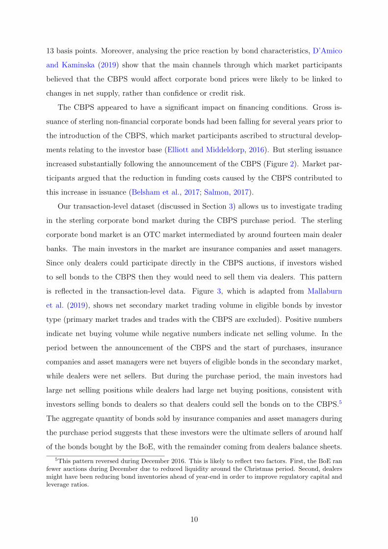
13 basis points. Moreover, analysing the price reaction by bond characteristics, D’Amico

and Kaminska (2019) show that the main channels through which market participants

believed that the CBPS would affect corporate bond prices were likely to be linked to

changes in net supply, rather than confidence or credit risk.

The CBPS appeared to have a significant impact on financing conditions. Gross is-

suance of sterling non-financial corporate bonds had been falling for several years prior to

the introduction of the CBPS, which market participants ascribed to structural develop-

ments relating to the investor base (Elliott and Middeldorp, 2016). But sterling issuance

increased substantially following the announcement of the CBPS (Figure 2). Market par-

ticipants argued that the reduction in funding costs caused by the CBPS contributed to

this increase in issuance (Belsham et al., 2017; Salmon, 2017).

Our transaction-level dataset (discussed in Section 3) allows us to investigate trading

in the sterling corporate bond market during the CBPS purchase period. The sterling

corporate bond market is an OTC market intermediated by around fourteen main dealer

banks. The main investors in the market are insurance companies and asset managers.

Since only dealers could participate directly in the CBPS auctions, if investors wished

to sell bonds to the CBPS then they would need to sell them via dealers. This pattern

is reflected in the transaction-level data. Figure 3, which is adapted from Mallaburn

et al. (2019), shows net secondary market trading volume in eligible bonds by investor

type (primary market trades and trades with the CBPS are excluded). Positive numbers

indicate net buying volume while negative numbers indicate net selling volume. In the

period between the announcement of the CBPS and the start of purchases, insurance

companies and asset managers were net buyers of eligible bonds in the secondary market,

while dealers were net sellers. But during the purchase period, the main investors had

large net selling positions while dealers had large net buying positions, consistent with

investors selling bonds to dealers so that dealers could sell the bonds on to the CBPS.5

The aggregate quantity of bonds sold by insurance companies and asset managers during

the purchase period suggests that these investors were the ultimate sellers of around half

of the bonds bought by the BoE, with the remainder coming from dealers balance sheets.

5This pattern reversed during December 2016. This is likely to reflect two factors. First, the BoE ranfewer auctions during December due to reduced liquidity around the Christmas period. Second, dealersmight have been reducing bond inventories ahead of year-end in order to improve regulatory capital andleverage ratios.

10

2.4 How might the CBPS have impacted liquidity?

Market participants and academics have proposed several mechanisms by which central

bank asset purchases could impact liquidity. In theory, the impact on liquidity could be

positive or negative.

Stimulating trading: Central bank asset purchases involve market participants selling

bonds in exchange for cash. But cash and bonds are imperfect substitutes, so the initial

purchases are likely to stimulate further portfolio rebalancing (Joyce et al., 2011a). By

stimulating trading, this portfolio rebalancing could also improve liquidity.

Reducing inventory risk: Dealers take risk by holding bonds on their balance sheets

as market-making inventory (Stoll, 1978). By providing a predictable source of demand

for bonds, asset purchases can reduce the inventory risk faced by dealers. This might

make them willing to hold larger inventories and could therefore facilitate market-making

(Kandrac, 2018).

Search frictions: Absent new issuance, asset purchases lead to a reduction in the

quantity of bonds held by private investors. If there are search frictions, then this could

reduce trading by making it more difficult for investors to be matched (Ferdinandusse

et al., 2017). And if it becomes more difficult for dealers to source specific bonds in the

secondary market, then the costs and risks of market-making could increase, reducing

dealers’ willingness to intermediate trades (Kandrac, 2018). Moreover, a reduction in

the quantity of a bond available for trading by private investors might deter market

participation, leading to a thinner market and lower liquidity (Bolton and von Thadden,

1998).

Distorted price signals: Central bank asset purchases typically involve quantity tar-

gets, making the central bank relatively price-insensitive in its purchase decisions. Market

participants have argued that this can distort price signals and therefore reduce the will-

ingness of investors to trade (Financial Times, 2015).

Market participants in the sterling corporate bond market generally argued that the

CBPS improved secondary market liquidity. The key channel that they emphasised was

11

a reduction in inventory risk: investors argued that predictable demand from the CBPS

made dealers more willing to hold market-making inventory (Belsham et al., 2017; Finan-

cial News, 2017). Over the rest of this paper, we aim to estimate the impact of the CBPS

on liquidity more formally.

3 Data

3.1 CBPS auction data

Our auction dataset includes the complete set of information determining CBPS pur-

chases. We observe granular information on each individual offer submitted, including:

the identity of the dealer, the ISIN (International Securities Identification Number) of the

bond, the offer quantity, the offer spread, the quantity of the offer that was accepted, and

the reason the offer was rejected (where applicable). We also observe the BoE’s reserve

spreads and purchase limits for each bond and each auction.

The dataset covers 82 auctions taking place over the lifetime of the scheme, from 27

September 2016 to 27 April 2017. Over that period, 364 bonds were eligible at some point

(issued by 144 issuers), 306 of which were purchased at least once.

Table 1 reports summary statistics for the auction data. For bonds that received at

least one offer in a given auction, the average sum of offer quantities was £9.2mn. For

bonds that were purchased in a given auction, the average total purchase size was around

£5mn. The maximum purchase amount of a single bond in a single auction was £10mn,

equal to the purchase limit.

As discussed in Section 2.2, the auction allocations were influenced by reserve spreads

set by the BoE. The distribution of reserve spreads is shown in Figure 4 (the chart pools

across bonds and auctions). The majority of reserve spreads were below the average

market mid spread. However, in some cases the reserve spreads were set substantially

higher than quoted market spreads in order to reduce the pace of purchases of particular

bonds.

12

3.2 Liquidity measures

Corporate bond transaction data

To estimate liquidity measures for the corporate bond market, we use the transaction-level

‘Zen’ dataset maintained by the UK Financial Conduct Authority (FCA). This dataset

includes transaction reports for all secondary-market trades by EEA-regulated firms in

corporate bonds that are issued by UK firms, and all secondary-market trades by UK-

regulated firms in any corporate bond. Since the large majority of the main dealers in

the sterling corporate bond market are UK-regulated firms, the dataset should cover the

majority of trading in sterling-denominated corporate bonds. And under the assumption

that most trading in euro-denominated bonds involves EEA-regulated dealers or investors,

the dataset should cover the majority of trading in euro-denominated bonds issued by UK

firms.

Each transaction report includes the date, time, ISIN, quantity, price, the identity of

the reporting firm, and (in most cases) the identity of their counterparty. The counter-

party information allows us to match reports in cases where both counterparties report

the trade. We drop trades that are implausibly large or small, or that have implausible

reported prices. We also drop trades that occur within one week of the bond’s announce-

ment date (trading volumes are much higher in the week after a bond is announced,

making this period unrepresentative of normal trading conditions in the bond).6

Corporate bond liquidity measures

We estimate market liquidity at the bond level. There is no single accepted liquid-

ity measure for bonds (Schestag et al., 2016). We therefore estimate a wide range of

transaction-based liquidity measures drawn from the academic literature. The measures

are summarised below and defined in Appendix A. We split the measures into three

groups: measures of trading activity, measures of transaction costs, and measures of price

impact.

Sterling and euro corporate bonds trade relatively infrequently, with around one trade

per day on average in the Zen dataset, so we compute all liquidity measures at weekly

6As discussed in Section 2.3, there was an increase in sterling corporate bond issuance after the CBPSwas announced. Given that bonds trade most frequently shortly after they are issued, the increase inissuance is likely to have caused an increase in average trading volumes. Since we drop trades around theissuance date, this effect should not affect our analysis.

13

frequency. We also winsorise several liquidity measures at 2.5% and 97.5% to reduce the

impact of outliers.7 Summary statistics for all the liquidity measures are provided in

Table 2 for the sample period January 2016 to December 2017.

Measures of trading activity. We compute four simple measures of trading activity:

weekly number of trades (COUNT), weekly sterling trading volume (VOLUME), average

trade size (SIZE), and weekly number of ‘large’ trades (LARGE).8 For these measures,

higher numbers are likely to indicate better liquidity. As reported in Table 2, the average

trade size for CBPS-eligible bonds is around £0.81mn, and eligible bonds trade on average

around 4.4 times per week. As shown in Figure 5, the measures of trading activity exhibit

substantial volatility but no clear trend over the sample period. The measures of trading

activity are cruder than the measures of transaction costs and price impact. But their

simplicity means that they can be estimated more reliably than the other measures, with

fewer missing observations.

Measures of transaction costs. We compute two measures of transaction costs: the

effective spread (SPREAD), and the Roll (1984) measure. These can be interpreted as

transaction-based estimates of the bid-ask spread. For these measures, higher numbers

indicate worse liquidity. These measures suggest that the average transaction-based bid-

ask spread of eligible bonds is between 25 and 40 basis points (Table 2). As shown in

Figure 6, both of these measures indicate that the liquidity of eligible bonds and ineligible

sterling investment grade bonds improved during the period in which CBPS purchases

occurred.

Measures of price impact. Finally we compute two measures of price impact: the

Amihud (2002) measure, and a simple implementation of the volatility-over-volume (VOV)

measure of Fong et al. (2017). For these measures, higher numbers indicate worse liquidity.

The Amihud measure indicates that, on average, a £1mn trade moves the price of eligible

bonds by around 83 basis points. Meanwhile, volatility-over-volume suggests that an

increase in trading volume of £1mn increases price volatility by around 26 basis points

(Table 2). As for the measures of transaction costs, both measures of price impact suggest

7We winsorise SPREAD, ROLL, AMIHUD and VOV.8We define a large trade to be one that is greater than £2mn, which is approximately the 90th

percentile of the trade size distribution.

14

that the liquidity of eligible bonds and ineligible sterling bonds improved substantially

over the CBPS purchase period (Figure 6).

While many of these measures indicate that liquidity in the sterling corporate bond

market improved as CBPS purchases took place, we cannot conclude that this improve-

ment was driven by the CBPS, because multiple other factors are likely to have also

impacted corporate bond liquidity during this period. For example, broader financial

market sentiment during this period was boosted by an improving outlook for global

economic growth, as well as accommodative monetary policy from both the European

Central Bank and the Bank of England (Bank of England, 2017c). In addition, the

improvement in liquidity might have been part of a longer-run trend of adjustment to

regulation. The introduction of post-crisis regulation such as the leverage ratio is likely

to have contributed to reductions in fixed income liquidity in the years before the launch

of the CBPS (Bicu-Lieb et al., 2020). However, over 2017, dealers were reported to have

improved their balance sheet optimization in response to these regulations, resulting in

improvements in the liquidity of fixed income markets, including corporate bonds (Bank

of England, 2017b).

These factors imply that we cannot simply interpret time series trends in corporate

bond liquidity as being caused by the CBPS. We therefore exploit weekly cross-sectional

variation across bonds to identify the impact of the CBPS purchases, as explained in

Section 5.

4 Announcement effects

Before estimating the impact of the purchases on liquidity, we investigate whether the an-

nouncement of the CBPS itself had a direct impact on liquidity. Specifically, we estimate

the following cross-sectional regression:

∆Liquidityb = µ+ βEligibleb + φ′Controlsb + εb, (1)

where ∆Liquidityb is the liquidity of bond b in the calendar week after the announcement

(8 – 12 August) minus liquidity in the calendar week before the announcement (25 – 29

July); and Controlsb is a set of bond-level variables measured prior to the announcement:

15

amount outstanding, credit rating, residual maturity, residual maturity squared, industry

fixed effects, yield spread to the reference government bond, and amount outstanding of

gilts with a similar residual maturity (within two years).

The variable of interest is Eligibleb, which is an indicator variable equal to one for

bonds that were eligible for purchase by the CBPS and zero otherwise.9 We consider

two control groups: sterling-denominated investment grade bonds that were never eligible

(bonds issued by banks and insurance companies are excluded), and euro-denominated

bonds issued by firms who had also issued eligible bonds.

The results are summarised in Table 3. There is evidence of significantly increased

trading activity in eligible bonds relative to euro-denominated bonds. This might have

reflected investor positioning ahead of the purchase period, as illustrated in Figure 3.

However the estimated coefficients on the transaction cost and price impact measures are

statistically insignificant in most cases, suggesting that the initial announcement did not

cause an immediate change in the costs of trading.

5 Impact of CBPS purchases on liquidity

5.1 Identification

We now estimate the impact of the CBPS purchases on liquidity. In doing so, we address

a general identification challenge faced by any study of the impact of central bank asset

purchases on liquidity, deriving from the fact that asset purchases are not randomly

assigned across bonds. Suppose that liquidity is determined by the following equation:

Lbt = αb + µt + βPbt + δᵀZbt + ebt, (2)

where Lbt denotes the liquidity of bond b in period t, Pbt denotes asset purchases, and Zbt is

a vector of other variables that impact liquidity. Importantly, Zbt could include variables

that are observed by market participants but not by the econometrician, notably market

participants’ expectations for liquidity. The identification challenge arises if purchases are

also affected by these variables: for example, market participants might be more willing to

9Although the list of eligible bonds was not published at the time of the announcement, the maineligibility criteria were published, and Boneva et al. (2018) show that the spreads of eligible bonds fellsignificantly more than the spreads of ineligible sterling bonds after the announcement, indicating thatinvestors were to a large extent able to predict which bonds would be eligible.

16

sell bonds that they expect to become less liquid; the central bank might avoid purchasing

bonds that it expects to become less liquid in order to protect its own balance sheet; or

the central bank might focus puchases on less liquid bonds in an attempt to improve the

liquidity of those bonds. Indeed, Song and Zhu (2014) and Schlepper et al. (2020) both

find evidence that central bank asset purchase decisions are impacted by liquidity. In any

of these cases, there would be a problem of reverse causality, with liquidity impacting

purchases rather than purchases impacting liquidity, and so simply regressing liquidity

Lbt on purchases Pbt would result in a biased estimate of β. Importantly, this effect could

go in either direction.

The design of the CBPS and the granularity of our dataset offer novel ways to address

this challenge. In comparison to bilateral purchases, the auction design of the CBPS

greatly reduces the discretionary nature of purchases. Moreover, the auction dataset

provides us with the complete set of information determining purchases — including

auction participants’ offers and the BoE’s reserve spreads and purchase limits. This

allows us to construct variables to isolate the impact of liquidity on purchases.

We take two main approaches, described in detail below. First, we use data on auc-

tion offers and reserve spreads to construct variables to directly control for the potential

channels of reverse causality from liquidity to purchases (Section 5.2). Second, we use

data on purchase limits and historical purchases to construct an instrument for current

purchases (Section 5.3).

5.2 Controlling for supply and demand factors

Specification

As explained above, CBPS purchases were not randomly assigned across bonds, but were

instead determined by the intersection of auction participants’ supply and the BoE’s

demand. Both of these might have been impacted by liquidity considerations, raising the

possiblity of reverse causality. However, given that purchases were made via auctions,

we are able to observe and therefore control for granular measures of both the supply

and demand factors determining purchases. We observe all of the individual offers by

market participants to sell bonds to the BoE, and can therefore use this information

to construct bond-level proxies for the strength of auction participants’ supply in each

auction. We construct two such proxies: one based on quantity (the total quantity of

17

the bond offered in the auction) and one based on price (the average spread between the

offer yields in the auction and the offer yield quoted in the market). Similarly, we use the

BoE’s bond-level reserve spread as a proxy to control for the strength of its demand for

the bond. By including these demand and supply proxies in our regressions, we are able

to directly control for the two potential channels of reverse causality. This argument is

set out formally in Appendix B.

Specifically, we run staggered difference-in-differences regressions at the bond-auction

level. Each regression uses data for bonds in a treatment group and bonds in a control

group, and takes the following form:

Liquiditybt = αb + µt + βPurchasedAmountbt + κXDemandbt + δ′XSupply

bt + εbt, (3)

where:

• Liquiditybt is a measure of secondary market liquidity for bond b in the week starting

immediately after auction t.

• αb and µt are bond and auction fixed effects.

• PurchasedAmountbt is the total nominal quantity of bond b purchased in auction t,

denominated in sterling millions.

• XDemandbt is the BoE’s reserve spread for bond b in auction t, which we use as a proxy

variable for the BoE’s demand for the bond.

• XSupplybt is a vector of two variables summarising the supply by auction participants

of bond b in auction t: the total nominal quantity offered in the auction (summed

across all auction participants); and the volume-weighted average spread between

auction participants’ offer yields and the average offer yield quoted in the secondary

market.

The coefficient of interest is β. This provides an estimate of the impact of CBPS

purchases on the liquidity of purchased bonds in the week following the auction.

We run separate regressions for different liquidity measures and different control

groups (discussed below). In each case, the treatment group consists of bonds for which

PurchasedAmountbt is greater than zero, i.e. bonds that were purchased in auction t.

18

Note that bonds can be treated multiple times because they can be purchased in multiple

auctions. Standard errors are double-clustered at the bond and auction levels.

Control groups

For robustness, we consider four different control groups. Our benchmark control group

(Offer) consists of bonds that were eligible in auction t and received offers, but were

not purchased (either because the offer spreads were below the reserve spread or because

purchase limits were reached). Note that bonds frequently move between the treatment

group and this control group depending on whether they have offers accepted. That is,

treatment status is determined within each auction, and bonds in the treatment group on

one date are likely to be in the control group on other dates. The identifying assumption

is that — in the absence of purchases, and conditional on demand and supply — the

liquidity of purchased bonds would have moved in line with the liquidity of this control

group: the ‘parallel trends’ assumption. This is very plausible, given that the BoE’s

eligibility criteria ensured that the bonds in the treatment and control groups had similar

characteristics in terms of credit rating, sector, and geographical focus.10

Our second control group (Limit) is a subset of the first. It consists of bonds that

were eligible in auction t and received offers in which the offer spread was greater than the

reserve spread (that is, attractive to the BoE), but were not purchased because auction

or issuer purchase limits were reached within the auction. Given that these offers were

at attractive prices, it would have been particularly difficult for auction participants to

predict that they would be rejected. Including this control group acts as a robustness

test against the possibility that auction participants were using sophisticated bidding

strategies that are not well approximated by our two proxy variables for supply.

The bonds in the Offer and Limit control groups are likely to be close substitutes

to the bonds in the treatment group. This has the advantage that the parallel trends

assumption is likely to hold. However, it also raises the possibility that the impact of

purchases on the treatment group ‘spills over’ to the control group: investors who have

sold bonds to the CBPS might rebalance their portfolios into bonds in the control group,

and this might mean that the CBPS purchases also indirectly impact the liquidity of

10The parallel trends assumption cannot easily be visually inspected for this control group, given thatbonds frequently move between the treatment and control groups.

19

control bonds.11 In order to obtain estimates that are less likely to be impacted by these

spillover effects, we repeat the analysis using two control groups that are less similar to

the treatment group: sterling-denominated investment grade corporate bonds that were

never eligible for the CBPS (Sterling),12 and euro-denominated bonds issued by issuers

who had also issued eligible bonds (Euro).

We can use Figures 5 and 6 to assess how well the parallel trends assumption holds

for these two additional control groups by observing trends in the liquidity measures

prior to the start of CBPS purchases. Over the pre-CBPS period, most of the liquidity

measures for eligible bonds and ineligible sterling bonds move relatively closely together,

providing support for the parallel trends assumption. The figures provide less support for

the parallel trends assumption in the case of the euro control group, which might reflect

differences in the investor base.

Sample construction

Eligible bonds were auctioned once per week, but different bonds were auctioned on

different weekdays depending on the sector of the issuer. So for eligible bonds (i.e. the

treatment group and the first two control groups), the regressions only use data from

auctions in which the bond was eligible. And we estimate the liquidity measures using

trades in the week starting on the day that the bond was auctioned, excluding the period

on the auction day before the close of the auction.

The Sterling and Euro control groups consist of ineligible bonds. We match each of

these bonds to auctions based on the sector of the issuer. We then estimate the liquidity

measures for these bonds in the same way as for eligible bonds, i.e. using trades in the

week starting on the day of the auction to which the bond was matched, excluding trades

before the close of the auction. Since these bonds are ineligible, purchased amount is

always equal to zero, and the demand and supply proxies are unobserved and therefore

excluded from the regressions.

11Note that spillover effects on control bonds might be expected to be in the same direction as thedirect effect on treated bonds, meaning that our difference-in-differences estimates might be expected tobe underestimates of the true effect.

12Bonds issued by banks and insurance companies are excluded.

20

Results

Our baseline results are summarised in Table 4. We run regressions for eight liquidity

measures and four control groups, resulting in a total of 32 regressions.

The results for the Offer control group are shown in Panel A. We find that trading

activity increased after CBPS purchases. Specifically, in response to a typical purchase of

£5mn, the number of weekly trades (COUNT) increases by around 1.4 (compared to an

average of 4.4 for eligible bonds over the sample period), weekly trading volume increases

by around £3.7mn (compared to an average of £3.5mn), the average trade size increases

by around £0.57mn (compared to an average of £0.81mn), and the number of large trades

(trades larger than £2mn) increases by around 0.46 (compared to an average of 0.45).

The measures of transaction costs also suggest that CBPS purchases improved liquid-

ity. A typical purchase of £5mn is associated with a reduction in the effective spread of

around 4.3 basis points (compared to an average of 26 basis points), and a reduction in

the Roll measure of the bid-ask spread of 1.8 basis points (compared to an average of 41

basis points). We also find that the CBPS reduced the price impact of trades. Following

a £5mn purchase, the Amihud measure falls by 4.1 basis points (compared to an average

of 83 basis points), and the volatility-over-volume measure falls by around 3.4 basis points

(compared to an average of 26 basis points).

The results using the other three control groups (Panels B, C and D) are very similar.

Overall these results provide robust evidence that the CBPS purchases improved the

liquidity of purchased bonds. This is consistent with reports from market participants

in the sterling corporate bond market. The key channel that they emphasised was a

reduction in inventory risk: predictable demand from the CBPS made dealers more willing

to hold market-making inventory and intermediate trades (Belsham et al., 2017; Financial

News, 2017).

Robustness tests

In Table 5, we include the lagged dependent variable (i.e. lagged liquidity) as an addi-

tional control variable, using the system GMM estimator of Blundell and Bond (1998).

The results are similar to our baseline results. Statistical significance is reduced in a

small number of regressions, which could reflect a reduction in efficiency arising from the

instrumental variables approach. The coefficient on lagged liquidity is generally relatively

21

small.

We perform three further robustness tests. First, we re-estimate the baseline regres-

sions for the Offer and Limit control groups, but exclude the proxy variables for demand

and supply. Second, we scale the treatment variable (purchased amount) by amount out-

standing, to allow for the possibility that the effect of purchases depends on the quantity

of the bond in issue. Third, we repeat the analysis using the common correlated effects

(CCE) estimator of Pesaran (2006), which controls for unobserved common shocks to

both purchases and liquidity. The results from all of these robustness tests (available in

Appendix C) are similar to our baseline results.

5.3 Instrumental variables approach

Our second identification strategy follows an instrumental variables approach. We drop

the supply and demand proxies to give the following equation of interest:

Liquiditybt = αb + µt + βPurchasedAmountbt + εbt. (4)

We then instrument PurchasedAmountbt using the proportion of the bond-level purchase

limit still available for purchase; that is:

PurchaseLimitbt − CurrentHoldingbt

PurchaseLimitbt

This instrument should be relevant because it affected the probability that bond b would

be purchased in auction t, by acting as a constraint on purchases. And it should be

exogenous, because it was determined mechanically based on amounts outstanding and

past purchases, and was not affected by other risk management or liquidity considerations.

We consider three control groups: bonds that were eligible in auction t but were not

purchased (either because they received no offers or because the offers were not accepted),

plus the Offer and Limit control groups described in Section 5.2.

The IV results are summarised in Table 6. The instrument is strong, with a first-stage

F -statistic above 60 in all regressions. The second-stage results are similar to the results

using the supply and demand proxies. For most liquidity measures, we find that purchases

improved liquidity, although for some liquidity measures there is a reduction in statistical

significance.

22

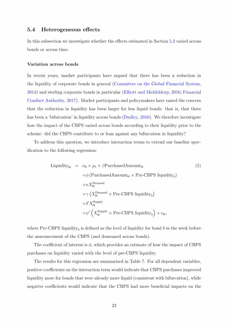
5.4 Heterogeneous effects

In this subsection we investigate whether the effects estimated in Section 5.2 varied across

bonds or across time.

Variation across bonds

In recent years, market participants have argued that there has been a reduction in

the liquidity of corporate bonds in general (Committee on the Global Financial System,

2014) and sterling corporate bonds in particular (Elliott and Middeldorp, 2016; Financial

Conduct Authority, 2017). Market participants and policymakers have raised the concern

that the reduction in liquidity has been larger for less liquid bonds: that is, that there

has been a ‘bifurcation’ in liquidity across bonds (Dudley, 2016). We therefore investigate

how the impact of the CBPS varied across bonds according to their liquidity prior to the

scheme: did the CBPS contribute to or lean against any bifurcation in liquidity?

To address this question, we introduce interaction terms to extend our baseline spec-

ification to the following regression:

Liquiditybt = αb + µt + βPurchasedAmountbt (5)

+φ (PurchasedAmountbt × Pre-CBPS liquidityb)

+κXDemandbt

+γ(XDemand

bt × Pre-CBPS liquidityb

)+δ′XSupply

bt

+ψ′(XSupply

bt × Pre-CBPS liquidityb

)+ εbt,

where Pre-CBPS liquidityb is defined as the level of liquidity for bond b in the week before

the announcement of the CBPS (and demeaned across bonds).

The coefficient of interest is φ, which provides an estimate of how the impact of CBPS

purchases on liquidity varied with the level of pre-CBPS liquidity.

The results for this regression are summarised in Table 7. For all dependent variables,

positive coefficients on the interaction term would indicate that CBPS purchases improved

liquidity more for bonds that were already more liquid (consistent with bifurcation), while

negative coefficients would indicate that the CBPS had more beneficial impacts on the

23

liquidity of less liquid bonds. We find that almost all estimated coefficients on the inter-

action between purchases and pre-CBPS liquidity are small and statistically insignificant.

Overall, these results do not indicate that the impact of the CBPS differed systematically

across purchased bonds.

Variation across time

The strength of the channels from asset purchases to liquidity discussed in Section 2.4 is

likely to depend on time-varying factors such as the expected time until completion of the

scheme. We therefore estimate whether the size of the impact of purchases on liquidity

established in Section 5.2 varied over the lifetime of the scheme. To that end, we estimate

the following regression:

Liquiditybt = αb + µt + βPurchasedAmountbt (6)

+φ (PurchasedAmountbt × Trendt)

+κXDemandbt

+γ(XDemand

bt × Trendt

)+δ′XSupply

bt

+ψ′(XSupply

bt × Trendt

)+ εbt,

where Trendt is a linear time trend variable at weekly frequency (defined to be zero at

the midpoint of the purchase period).

The results are summarised in Table 8. For the measures of trading activity (COUNT,

VOLUME, SIZE, LARGE), the estimated coefficient on the interaction between purchased

amount and the time trend is generally negative and significant. This indicates that

the positive impact of CBPS purchases on trading activity decreased over the purchase

period. For the other liquidity measures, the estimated coefficient on the interaction term

is statistically insignificant for most control groups.

The reduced impact on trading activity might have reflected a weakening in the in-

ventory risk channel over the course of the scheme. As the CBPS approached its £10bn

purchase target, the future time period over which dealers would be able to sell excess

inventory to the CBPS reduced. Therefore the reduction in inventory risk associated with

the CBPS might have dissipated, potentially reducing the positive impact of the CBPS

24

on dealers’ willingness to intermediate trades.

6 Stock effects of CBPS on liquidity

The results in Section 5 indicate that CBPS purchases improved the liquidity of bonds

in the week following the purchase. In other words — and following the terminology of

D’Amico and King (2013) — we find that the CBPS had ‘flow effects’ on bond liquidity.

We now turn to the question of whether the purchases also had longer-lasting ‘stock

effects’ on liquidity by comparing how the liquidity of bonds changed between the start

and end of purchases.

Specifically, we run cross-sectional regressions of the form:

∆Liquidityb = µ+ βTotalPuchasedAmountb + φ′Controlsb + εb, (7)

where ∆Liquidityb is the liquidity of bond b in the week after purchases were completed

minus liquidity in the week before the CBPS was announced. The variable of interest

is TotalPurchasedAmountb, which is defined as the total quantity of bond b purchased

by the CBPS over the entire purchase period. We include several bond-specific control

variables measured just before the announcement of the CBPS: amount outstanding,

credit rating, residual maturity, residual maturity squared, industry fixed effects, yield

spread to reference gilt, and amount outstanding of gilts with a similar residual maturity.13

We also include bond-level control variables computed over the duration of the scheme:

change in credit rating, change in amount outstanding of gilts with a similar residual

maturity, and BoE QE purchases of gilts with a similar maturity.

The treatment group is bonds that were purchased during the CBPS period. We

consider two control groups: bonds that were eligible but never purchased, and ineli-

gible sterling investment grade corporate bonds (bonds issued by banks and insurance

companies are excluded).

The results are shown in Table 9. In almost all cases, the estimated impact of total

purchases on liquidity is statistically insignificant. This suggests that the liquidity effects

of the CBPS did not extend beyond the active phase of purchases. That is, although

the CBPS had beneficial ‘flow effects’ on bond liquidity, there were no ‘stock effects’

13Specifically, gilts with a residual maturity within two years of the residual maturity of bond b.

25

arising from the BoE’s total holdings of corporate bonds. This is consistent with the

inventory risk channel discussed in Section 2.4: the CBPS might have supported liquidity

by providing a committed buyer to the market, but this impact did not persist once CBPS

purchases were completed.

In this respect, our findings are in line with Christensen and Gillan (2017), who study

the impact of the Federal Reserve’s purchases of TIPS on liquidity premia during QE2.

They find that TIPS liquidity premia fell during the program, but that the effects dissi-

pated towards the end of the purchases. They conclude that, although QE can improve

financial market functioning through a liquidity channel, the liquidity effects are only

sustained as long as purchases are ongoing and expected to continue.

7 Discussion and conclusions

Identifying the impact of central bank asset purchases on liquidity is plagued with en-

dogeneity concerns, particularly the possibility of reverse causality. For example, if the

central bank aims to purchase more or less liquid bonds, then liquidity will be impacting

purchases as well as purchases impacting liquidity. In order to address this identification

challenge, we study the Bank of England’s Corporate Bond Purchase Scheme (CBPS),

in which the BoE purchased £10bn of sterling corporate bonds via a series of auctions

over 2016 and 2017. To estimate the impact of the purchases on liquidity, we create a

novel dataset by combining transaction-level data from the corporate bond market with

proprietary offer-level data from the CBPS auctions.

The auction design of the CBPS and the granularity of our auction dataset offer novel

ways to alleviate the reverse causality problem. In particular, we are able to control for the

impact of liquidity on purchases by constructing proxy variables for auction participants’

supply of bonds (based on their offers in the auctions) and the BoE’s demand for bonds

(based on the reserve prices that it set ahead of the auctions).

We find that CBPS purchases improved the liquidity of purchased bonds in the week

following the purchase. This result is robust across a range of transaction-based liquidity

measures, control groups, and identification strategies. However, when we compare the

overall change in liquidity between the start and end of the scheme, we find no evidence

that the liquidity of purchased bonds changed systematically compared to sterling bonds

26

that were not purchased.

The fact that we observe positive short-run effects on liquidity, but do not observe sig-

nificant long-run effects, could reflect the relatively small size of the scheme. Theoretically,

the positive channels through which QE might impact liquidity — namely by stimulating

trading and reducing inventory risk — could operate even for small purchases. Meanwhile,

the potential negative channels — increased search frictions and distorted price signals

— are more likely to become important when the stock of purchases is relatively large.

This possibility would reconcile our results with those of Kandrac (2018), who finds that

the Federal Reserve’s (much larger) purchases of mortgage-backed securities had negative

impacts on liquidity.

Our results have important policy implications. Policymakers and market participants

have repeatedly raised concerns that asset purchases could have the unintended conse-

quence of causing a deterioration in liquidity. Our results provide evidence that, in the

case of the CBPS, the purchases caused an improvement, rather than a deterioration, in

liquidity. At the margin, this should make central banks more willing to implement QE in

the future. While our empirical tests are not designed to sharply differentiate between the

different channels through which asset purchases can impact liquidity, the results appear

consistent with a scenario in which the purchases provided dealers with confidence that

they could sell bonds to the BoE if needed, and thereby increased dealers’ willingness to

hold inventory and intermediate trades. This channel might have been strengthened by

the fact that the purchases were implemented via auction, which increased transparency

and gave dealers more influence over which bonds would be bought, compared to an

operational design in which the central bank purchases bonds bilaterally.

The CBPS is a monetary policy tool, and did not have an explicit objective of im-

proving market liquidity. However, since the financial crisis, policymakers and academics

have paid increased attention to the question of whether, and under what conditions, the

central bank should act as ‘market-maker of last resort’ (MMLR) in markets suffering a

reduction in liquidity (BIS, 2014). The results in this paper indicate that asset purchases

conducted via auction can improve the liquidity of corporate bond markets and therefore

have implications for the design of any future MMLR operations.

27

References

Aigner, D. J., C. Hsiao, A. Kapteyn, and T. Wansbeek (1984): “Latent variable

models in econometrics,” in Handbook of Econometrics, ed. by Z. Griliches and M. D.

Intriligator, Elsevier, vol. 2, chap. 23, 1321–1393, 1 ed.

Amihud, Y. (2002): “Illiquidity and stock returns: cross-section and time-series effects,”

Journal of Financial Markets, 5, 31–56.

Bank of England (2016): “Inflation Report,” August.

——— (2017a): “Asset Purchase Facility: Corporate Bond Purchase Scheme - Consoli-

dated Market Notice,” Market Notice.

——— (2017b): “Financial Stability Report,” November.

——— (2017c): “Markets and operations - 2017 Q1,” Bank of England Quarterly Bulletin,

57, 50–58.

Belsham, T., A. Rattan, and R. Maher (2017): “Corporate Bond Purchase Scheme:

design, operation and impact,” Bank of England Quarterly Bulletin, 57, 170–181.

Bernanke, B. (2012): “Monetary Policy since the Onset of the Crisis,” Remarks at the

Federal Reserve Bank of Kansas City Economic Symposium at Jackson Hole, Wyoming.

Bicu-Lieb, A., L. Chen, and D. Elliott (2020): “The leverage ratio and liquidity

in the gilt and gilt repo markets,” Journal of Financial Markets, 48, 1–29.

BIS (2014): “Re-thinking the lender of last resort,” BIS Papers 79, Bank for International

Settlements.

Blundell, R. and S. Bond (1998): “Initial conditions and moment restrictions in

dynamic panel data models,” Journal of Econometrics, 87, 115–143.

Bolton, P. and E.-L. von Thadden (1998): “Blocks, Liquidity, and Corporate Con-

trol,” Journal of Finance, 53, 1–25.

Boneva, L., C. de Roure, and B. Morley (2018): “The impact of the Bank of Eng-

land’s Corporate Bond Purchase Scheme on yield spreads,” Bank of England working

papers 719, Bank of England.

28

Christensen, J. and J. Gillan (2017): “Does Quantitative Easing Affect Market

Liquidity?” Working Paper Series 2013-26, Federal Reserve Bank of San Francisco.

Committee on the Global Financial System (2014): “Market-making and pro-

prietary trading: industry trends, drivers and policy implications,” CGFS Papers 52,

Bank for International Settlements.

D’Amico, S. and I. Kaminska (2019): “Credit easing versus quantitative easing: ev-

idence from corporate and government bond purchase programs,” Bank of England

working papers 825, Bank of England.

D’Amico, S. and T. King (2013): “Flow and stock effects of large-scale treasury

purchases: evidence on the importance of local supply,” Journal of Financial Economics,

108, 425–448.

De Pooter, M., R. F. Martin, and S. Pruitt (2018): “The Liquidity Effects of

Official Bond Market Intervention,” Journal of Financial and Quantitative Analysis,

53, 243–268.

Dick-Nielsen, J., P. Feldhutter, and D. Lando (2012): “Corporate bond liquidity

before and after the onset of the subprime crisis,” Journal of Financial Economics, 103,

471–492.

Dudley, W. C. (2016): “Market and funding liquidity - an overview,” Speech.

Elliott, D. and M. Middeldorp (2016): “What explains the fall in sterling corporate

bond issuance?” Bank Underground, blog post.

Eser, F. and B. Schwaab (2016): “Evaluating the impact of unconventional monetary

policy measures: Empirical evidence from the ECB’s Securities Markets Programme,”

Journal of Financial Economics, 119, 147–167.

Ferdinandusse, M., M. Freier, and A. Ristiniemi (2017): “Quantitative easing

and the price-liquidity trade-off,” Working Paper Series 335, Sveriges Riksbank.

Financial Conduct Authority (2017): “New evidence on liquidity in UK corporate

bond markets,” February.

29

Financial News (2017): “Credit managers warn on liquidity as BoE buying nears its

end,” News article.

Financial Times (2015): “ECB’s buying challenges covered bonds,” News article.

Fisher, P. (2010): “The corporate sector and the Bank of England’s asset purchases,”

Speech.

Fong, K. Y. L., C. W. Holden, and O. Tobek (2017): “Are volatility over volume

liquidity proxies useful for global or US research?” Working Paper.

Han, F. and D. Seneviratne (2018): “Scarcity Effects of Quantitative Easing on Mar-

ket Liquidity: Evidence from the Japanese Government Bond Market,” IMF Working

Papers 18/96, International Monetary Fund.

Hong, G. and A. Warga (2000): “An empirical study of bond market transactions,”

Financial Analysts Journal, 56, 32–46.

Iwatsubo, K. and T. Taishi (2018): “Quantitative Easing and Liquidity in the

Japanese Government Bond Market,” International Review of Finance, 18, 463–475.

Joyce, M., A. Lasaosa, I. Stevens, and M. Tong (2011a): “The financial market

impact of quantitative easing in the United Kingdom,” International Journal of Central

Banking, 7, 113–161.

Joyce, M., M. Tong, and R. Woods (2011b): “The United Kingdom’s quantitative

easing policy: design, operation and impact,” Bank of England Quarterly Bulletin, 51,

200–212.

Kandrac, J. (2013): “Have Federal Reserve MBS purchases affected market function-

ing?” Economics Letters, 121, 188–191.

——— (2018): “The Cost of Quantitative Easing: Liquidity and Market Functioning

Effects of Federal Reserve MBS Purchases,” International Journal of Central Banking,

14, 259–304.

Kurosaki, T., Y. Kumano, K. Okabe, and T. Nagano (2015): “Liquidity in JGB

Markets: An Evaluation from Transaction Data,” Bank of Japan Working Paper Series

15-E-2, Bank of Japan.

30

Mallaburn, D., M. Roberts-Sklar, and L. Silvestri (2019): “Trading activity

during the Corporate Bond Purchase Scheme,” Bank Underground, blog post.

Pelizzon, L., M. G. Subrahmanyam, R. Tobe, and J. Uno (2018): “Scarcity

and Spotlight Effects on Liquidity and Yield: Quantitative Easing in Japan,” IMES

Discussion Paper Series 18-E-14, Institute for Monetary and Economic Studies, Bank

of Japan.

Pesaran, M. (2006): “Estimation and Inference in Large Heterogeneous Panels with a

Multifactor Error Structure,” Econometrica, 74, 967–1012.

Roll, R. (1984): “A Simple Implicit Measure of the Effective Bid-Ask Spread in an

Efficient Market,” Journal of Finance, 39, 1127–39.

Salmon, C. (2017): “Market Functioning,” Speech.

Schestag, R., P. Schuster, and M. Uhrig-Homburg (2016): “Measuring Liquidity

in Bond Markets,” Review of Financial Studies, 29, 1170–1219.

Schlepper, K., H. Hofer, R. Riordan, and A. Schrimpf (2020): “The Market Mi-

crostructure of Central Bank Bond Purchases,” Journal of Financial and Quantitative

Analysis, 55, 193–221.

Song, Z. and H. Zhu (2014): “QE Auctions of Treasury Bonds,” Finance and Eco-

nomics Discussion Series 2014-48, Board of Governors of the Federal Reserve System.

Steeley, J. (2015): “The side effects of quantitative easing: Evidence from the UK

bond market,” Journal of International Money and Finance, 51, 303–336.

Stoll, H. (1978): “The Supply of Dealer Services in Securities Markets,” Journal of

Finance, 33, 1133–51.

Todorov, K. (2020): “Quantify the Quantitative Easing: Impact on Bonds and Corpo-

rate Debt Issuance,” Journal of Financial Economics, 135, 340–358.

31

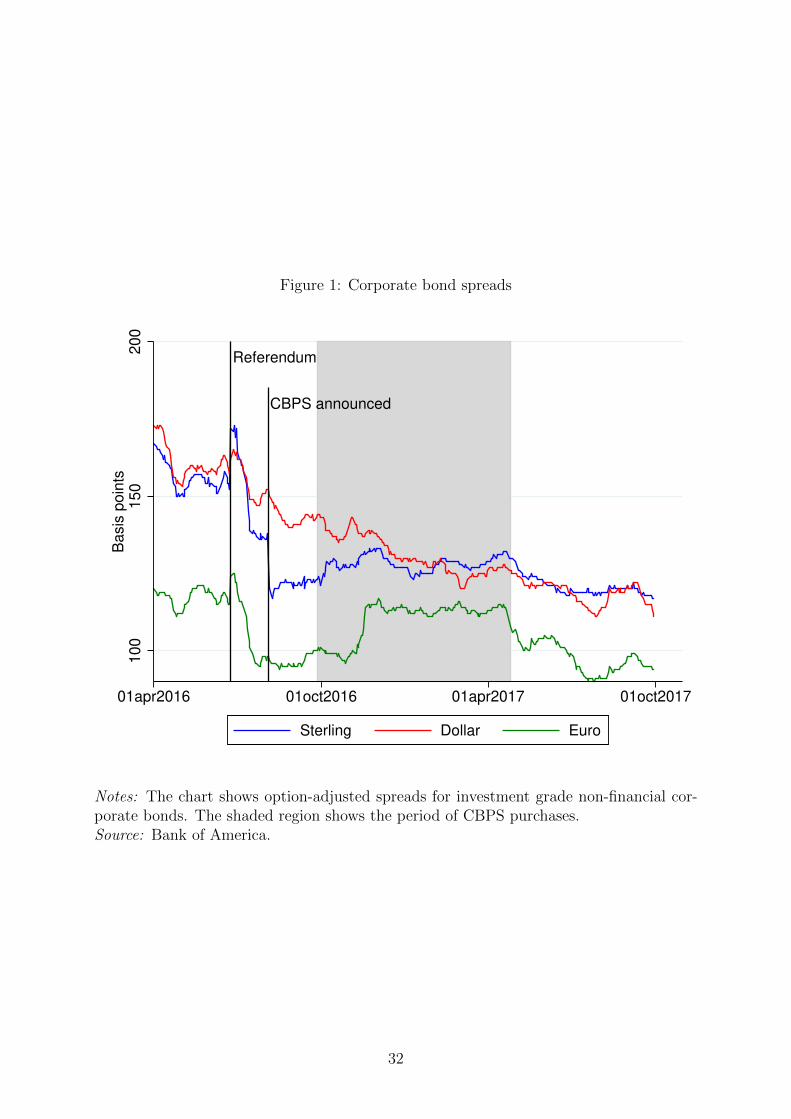
Figure 1: Corporate bond spreads

Referendum

CBPS announced

100

150

200

Basis

poin

ts

01apr2016 01oct2016 01apr2017 01oct2017

Sterling Dollar Euro

Notes: The chart shows option-adjusted spreads for investment grade non-financial cor-porate bonds. The shaded region shows the period of CBPS purchases.Source: Bank of America.

32

Figure 2: Sterling corporate bond issuance

CBPS announced

02

46

8

£ b

illions

2012m1 2014m1 2016m1 2018m1

Notes: The chart shows monthly gross issuance of sterling-denominated investment gradenon-financial corporate bonds.Source: Thomson Reuters.

33

Figure 3: Net trading in eligible corporate bonds

CBPS announced

−1

01

£ b

illio

ns

2016m1 2016m7 2017m1 2017m7 2018m1

Dealers

Asset managers and insurance companies

Others

Notes: The chart shows monthly net secondary market trading volumes in bonds thatwere eligible for the CBPS, estimated using the transaction-level Zen dataset. Primarymarket trades and trades with the CBPS itself are excluded. Positive numbers indicatenet buying volume while negative numbers indicate net selling volume. The shaded regionshows the period of CBPS purchases.

34

Figure 4: Distribution of reserve spreads

0200

400

600

800

Fre

quency

<−25 −20 −15 −10 −5 0 5 10 15 20 >25Reserve spread minus market mid (basis points)

Notes: The chart shows a histogram of the reserve spreads set by the Bank of Englandahead of CBPS auctions. Quoted market mid spreads have been subtracted from thereserve spreads. Spreads greater than 25 basis points are allocated to the highest bin, andspreads less than -25 basis points are allocated to the lowest bin.

35

Figure 5: Measures of trading activity

(a) Number of trades per week

Referendum

CBPS announced

05

10

15

2016m1 2016m7 2017m1 2017m7 2018m1

Eligible Ineligible sterling Euro

(b) Weekly trading volume (£mn)

Referendum

CBPS announced

24

68

10

2016m1 2016m7 2017m1 2017m7 2018m1

Eligible Ineligible sterling Euro

(c) Average trade size (£mn)

Referendum

CBPS announced

.4.6

.81

1.2

2016m1 2016m7 2017m1 2017m7 2018m1

Eligible Ineligible sterling Euro

(d) Number of large trades per week

Referendum

CBPS announced

.2.4

.6.8

1

2016m1 2016m7 2017m1 2017m7 2018m1

Eligible Ineligible sterling Euro

Notes: The charts show liquidity measures for the corporate bond market estimated usingthe transaction-level Zen dataset. The measures are computed for individual bonds atweekly frequency, then averaged across bonds within a group. The charts show monthlyaverages. ‘Eligible’ refers to bonds that were at some point eligible for the CBPS. ‘In-eligible sterling’ refers to sterling-denominated investment grade corporate bonds thatwere never eligible for the CBPS (bonds issued by banks and insurance companies areexcluded). ‘Euro’ refers to euro-denominated bonds issued by issuers who had also issuedeligible bonds. The shaded region shows the period of CBPS purchases. Higher numbersindicate better liquidity. Definitions of the measures are provided in Appendix A.

36

Figure 6: Measures of transaction costs and price impact

(a) Effective spread (bps)

Referendum

CBPS announced

10

20

30

40

2016m1 2016m7 2017m1 2017m7 2018m1

Eligible Ineligible sterling Euro

(b) Roll (bps)

Referendum

CBPS announced

20

30

40

50

60

2016m1 2016m7 2017m1 2017m7 2018m1

Eligible Ineligible sterling Euro

(c) Amihud (bps)

Referendum

CBPS announced

40

60

80

10

01

20

2016m1 2016m7 2017m1 2017m7 2018m1

Eligible Ineligible sterling Euro

(d) Volatility-over-volume (bps)

Referendum

CBPS announced

10

20

30

40

2016m1 2016m7 2017m1 2017m7 2018m1

Eligible Ineligible sterling Euro

Notes: The charts show liquidity measures for the corporate bond market estimated usingthe transaction-level Zen dataset. The measures are computed for individual bonds atweekly frequency, then averaged across bonds within a group. The charts show monthlyaverages. ‘Eligible’ refers to bonds that were at some point eligible for the CBPS. ‘In-eligible sterling’ refers to sterling-denominated investment grade corporate bonds thatwere never eligible for the CBPS (bonds issued by banks and insurance companies areexcluded). ‘Euro’ refers to euro-denominated bonds issued by issuers who had also issuedeligible bonds. The shaded region shows the period of CBPS purchases. Higher numbersindicate worse liquidity. Definitions of the measures are provided in Appendix A.

37

Table 1: Summary statistics: Auction variables

Statistic: N Mean Std dev Min Median Max

Total amount offered (GBP mn) 4,275 9.16 9.03 1.0 6.3 78.6

Average offer spread (bps) 4,275 1.25 4.63 -62.0 1.6 25.0

Total amount purchased (GBP mn) 1,622 4.83 3.29 0.1 4.0 10.0

Notes: The table shows summary statistics from the offer-level CBPS auction dataset.One observation refers to a bond-auction pair. ‘Total amount offered’ is the total quantityof a single bond offered by auction participants in a single auction, in nominal terms.‘Average offer spread’ is the volume-weighted average spread between auction participants’offer yields and the average offer yield quoted in the secondary market. ‘Total amountpurchased’ is the total quantity of a single bond purchased in a single auction, in nominalterms. The summary statistics for total amount offered and average offer spread arecomputed using observations where there was at least one offer for the bond in the auction.The summary statistics for total amount purchased are computed using observationswhere the bond was purchased in the auction.

38

Table 2: Summary statistics: Liquidity measures

Statistic: N Mean Std dev Min Median Max

Eligible bonds

COUNT 36,042 4.42 6.12 0.00 3.00 196.00

VOLUME (GBP mn) 36,042 3.53 7.19 0.00 0.94 274.40

SIZE (GBP mn) 27,383 0.81 1.11 0.00 0.48 27.64

LARGE 36,042 0.45 1.11 0.00 0.00 24.00

SPREAD (bps) 14,724 25.83 42.77 -61.82 18.13 140.53

ROLL (bps) 14,781 40.90 47.26 0.00 25.15 186.73

AMIHUD (bps) 20,063 83.29 103.90 0.00 44.08 442.22

VOV (bps) 14,781 25.95 30.05 0.94 15.04 132.73

Ineligible sterling investment grade bonds

COUNT 52,166 2.81 6.88 0.00 0.00 156.00

VOLUME (GBP mn) 52,166 2.16 6.35 0.00 0.00 158.30

SIZE (GBP mn) 20,161 0.86 1.36 0.00 0.50 29.97

LARGE 52,166 0.27 0.94 0.00 0.00 27.00

SPREAD (bps) 11,437 25.82 41.11 -61.82 18.48 140.53

ROLL (bps) 11,614 37.45 42.49 0.00 24.14 186.73

AMIHUD (bps) 15,459 81.76 101.04 0.00 44.26 442.22

VOV (bps) 11,614 21.19 25.90 0.94 12.18 132.73

Euro-denominated bonds issued by eligible issuers

COUNT 56,659 8.15 14.42 0.00 4.00 610.00

VOLUME (GBP mn) 56,659 5.23 11.14 0.00 1.31 322.89

SIZE (GBP mn) 39,896 0.66 0.89 0.00 0.44 27.04

LARGE 56,659 0.59 1.54 0.00 0.00 53.00

SPREAD (bps) 25,432 14.32 29.15 -61.82 9.98 140.53

ROLL (bps) 29,930 23.70 28.69 0.00 14.90 186.73

AMIHUD (bps) 32,176 46.32 61.80 0.00 26.64 442.22

VOV (bps) 29,930 12.15 17.33 0.94 6.96 132.73

Notes: The table shows summary statistics for corporate bond liquidity measures esti-mated using the transaction-level Zen dataset. The measures are computed at the bondlevel and at weekly frequency. The sample period is January 2016 to December 2017.Definitions of the measures are provided in Appendix A. SPREAD, ROLL, AMIHUDand VOV are winsorised at 2.5% and 97.5%.

39

Table 3: Announcement effects

(1) (2) (3) (4) (5) (6) (7) (8)

Liquidity measure: COUNT VOLUME SIZE LARGE SPREAD ROLL AMIHUD VOV

Panel A: Sterling control group

Eligible 0.185 0.711 -0.064 0.095 5.106 2.618 -16.562 -2.657

(0.831) (0.932) (0.170) (0.142) (10.069) (9.619) (21.919) (5.701)

Observations 545 545 316 545 136 154 226 154

R2 0.085 0.107 0.028 0.084 0.079 0.114 0.058 0.093

Panel B: Euro control group

Eligible 3.026∗ 4.530∗∗∗ 0.240∗ 0.451∗∗ 22.446∗∗∗ -7.351 -14.164 -6.172∗

(1.547) (1.568) (0.128) (0.217) (7.277) (6.528) (13.290) (3.343)

Observations 690 690 505 690 213 287 355 287

R2 0.153 0.098 0.016 0.092 0.099 0.039 0.081 0.056

Notes: The table shows regression results for equation (1). The regressions are estimatedat the bond level. The dependent variable is the change in liquidity from the weekbefore the CBPS was announced (25 – 29 July 2016) to the week after the CBPS wasannounced (8 – 12 August 2016). Different columns correspond to different liquiditymeasures. ‘Eligible’ is an indicator variable equal to one for bonds that were eligiblefor purchase by the CBPS, and zero otherwise. All regressions include the followingbond-level controls (measured before the announcement): amount outstanding, creditrating, residual maturity, residual maturity squared, industry fixed effects, yield spreadto the reference government bond, and amount outstanding of gilts with a similar residualmaturity (within two years). Control groups are defined in Section 4. Standard errors arerobust to heteroskedasticity and reported in parentheses. ∗∗∗, ∗∗, and ∗ indicate significanceat 1%, 5%, and 10%, respectively.

40

Table 4: Impact of CBPS purchases on liquidity

(1) (2) (3) (4) (5) (6) (7) (8)

Liquidity measure: COUNT VOLUME SIZE LARGE SPREAD ROLL AMIHUD VOV

Panel A: Offer control group

Amount purchased 0.289∗∗∗ 0.739∗∗∗ 0.114∗∗∗ 0.091∗∗∗ -0.854∗∗ -0.357∗ -0.828∗ -0.684∗∗∗

(0.045) (0.057) (0.013) (0.009) (0.347) (0.180) (0.462) (0.114)

Observations 4266 4266 3915 4266 2539 2620 3320 2620

R2 0.431 0.309 0.280 0.237 0.206 0.323 0.280 0.490

Panel B: Limit control group

Amount purchased 0.246∗∗∗ 0.776∗∗∗ 0.142∗∗∗ 0.090∗∗∗ -0.850∗ -0.693∗∗ -2.080∗∗∗ -0.877∗∗∗

(0.059) (0.068) (0.017) (0.010) (0.428) (0.306) (0.566) (0.135)

Observations 2579 2579 2399 2579 1575 1611 2052 1611

R2 0.441 0.368 0.366 0.286 0.258 0.342 0.321 0.543

Panel C: Sterling control group

Amount purchased 0.385∗∗∗ 0.978∗∗∗ 0.145∗∗∗ 0.108∗∗∗ -0.950∗ -0.537 -2.742∗∗∗ -0.941∗∗∗

(0.064) (0.066) (0.020) (0.009) (0.512) (0.368) (0.704) (0.128)

Observations 14594 14594 6546 14594 3880 3932 5221 3932

R2 0.623 0.394 0.325 0.319 0.224 0.291 0.280 0.560

Panel D: Euro control group

Amount purchased 0.389∗∗∗ 0.978∗∗∗ 0.144∗∗∗ 0.110∗∗∗ -0.887∗ -0.407 -2.301∗∗∗ -0.847∗∗∗

(0.062) (0.065) (0.020) (0.009) (0.491) (0.371) (0.692) (0.150)

Observations 16540 16540 12240 16540 7824 9190 10096 9190

R2 0.604 0.468 0.291 0.397 0.203 0.275 0.293 0.506

Notes: The table shows regression results for equation (3). The regressions are estimatedat the bond-auction level. The dependent variable is liquidity in the week starting onthe day of the auction. Different columns correspond to different liquidity measures.‘Amount purchased’ is the total nominal quantity of the bond purchased in the auction,denominated in sterling millions. All regressions include bond and auction fixed effects.Control groups are defined in Section 5.2. The regressions using the Offer and Limitcontrol groups include proxy variables for the BoE’s demand and auction participants’supply (defined in Section 5.2). The sample period is September 2016 to April 2017.Standard errors are double-clustered at the bond and auction levels, and reported inparentheses. ∗∗∗, ∗∗, and ∗ indicate significance at 1%, 5%, and 10%, respectively.

41

Table 5: Impact of CBPS purchases on liquidity – controlling for lagged liquidity

(1) (2) (3) (4) (5) (6) (7) (8)

Liquidity measure: COUNT VOLUME SIZE LARGE SPREAD ROLL AMIHUD VOV

Panel A: Offer control group

Amount purchased 0.257∗∗∗ 0.716∗∗∗ 0.085∗∗∗ 0.084∗∗∗ -0.882 -0.503 -1.158 -0.617∗∗∗

(0.050) (0.071) (0.013) (0.011) (0.595) (0.428) (0.801) (0.219)

Lagged liquidity 0.004 0.117∗∗∗ 0.006 0.084∗∗∗ 0.052 0.027 -0.047 0.062

(0.063) (0.033) (0.038) (0.028) (0.058) (0.047) (0.035) (0.064)

Observations 3933 3933 3364 3933 1605 1808 2554 1808

Panel B: Limit control group

Amount purchased 0.215∗∗∗ 0.697∗∗∗ 0.094∗∗∗ 0.086∗∗∗ -1.422∗ -0.330 -1.857∗∗ -0.764∗∗∗

(0.060) (0.082) (0.015) (0.013) (0.739) (0.549) (0.937) (0.278)

Lagged liquidity -0.022 0.130∗∗∗ -0.035 0.083∗∗ -0.024 -0.021 -0.084∗∗ 0.009

(0.083) (0.046) (0.046) (0.034) (0.077) (0.064) (0.043) (0.067)

Observations 2395 2395 2073 2395 1011 1131 1587 1131

Panel C: Sterling control group

Amount purchased 0.264∗∗∗ 0.600∗∗∗ 0.067∗∗∗ 0.073∗∗∗ -1.135∗∗ -0.923∗ -2.515∗∗∗ -0.969∗∗∗

(0.058) (0.074) (0.013) (0.012) (0.567) (0.496) (0.934) (0.252)

Lagged liquidity 0.113∗∗∗ 0.102∗∗∗ 0.007 0.062∗∗∗ -0.026 0.079∗ 0.020 0.076∗∗

(0.028) (0.023) (0.034) (0.021) (0.056) (0.041) (0.033) (0.038)

Observations 13559 13559 5324 13559 2347 2641 3787 2641

Panel D: Euro control group

Amount purchased 0.274∗∗∗ 0.614∗∗∗ 0.069∗∗∗ 0.074∗∗∗ -1.162∗∗ -0.778∗ -2.177∗∗ -0.774∗∗∗

(0.060) (0.074) (0.013) (0.012) (0.542) (0.445) (0.853) (0.243)

Lagged liquidity 0.126∗∗∗ 0.122∗∗∗ -0.000 0.067∗∗∗ -0.022 -0.003 -0.009 0.069∗

(0.034) (0.024) (0.024) (0.020) (0.031) (0.035) (0.026) (0.040)

Observations 15327 15327 10734 15327 5247 7019 7982 7019

Notes: The table shows regression results for equation (3). The regressions are estimatedat the bond-auction level using the system GMM estimator of Blundell and Bond (1998).The dependent variable is liquidity in the week starting on the day of the auction. Differ-ent columns correspond to different liquidity measures. ‘Amount purchased’ is the totalnominal quantity of the bond purchased in the auction, denominated in sterling millions.All regressions include bond and auction fixed effects. Control groups are defined in Sec-tion 5.2. The regressions using the Offer and Limit control groups include proxy variablesfor the BoE’s demand and auction participants’ supply (defined in Section 5.2). The sam-ple period is September 2016 to April 2017. Standard errors are double-clustered at thebond and auction levels, and reported in parentheses. ∗∗∗, ∗∗, and ∗ indicate significanceat 1%, 5%, and 10%, respectively.

42

Table 6: Impact of CBPS purchases on liquidity – instrumental variables

(1) (2) (3) (4) (5) (6) (7) (8)

Liquidity measure: COUNT VOLUME SIZE LARGE SPREAD ROLL AMIHUD VOV

Panel A: Eligible control group

Amount purchased 0.616∗∗∗ 1.461∗∗∗ 0.257∗∗∗ 0.200∗∗∗ 0.494 -1.592 -4.163∗∗ -2.292∗∗∗

(0.140) (0.168) (0.035) (0.028) (0.911) (0.968) (1.816) (0.480)

Observations 8381 8381 6627 8381 3746 3731 5088 3731

First-stage F -statistic 135.986 135.986 148.161 135.986 134.887 106.506 114.844 106.506

Panel B: Offer control group

Amount purchased 0.436∗∗ 1.224∗∗∗ 0.212∗∗∗ 0.156∗∗∗ -0.967 -2.048∗∗ -5.369∗∗ -1.640∗∗∗

(0.171) (0.189) (0.036) (0.032) (1.011) (0.900) (2.108) (0.442)

Observations 3927 3927 3621 3927 2358 2433 3082 2433

First-stage F -statistic 110.245 110.245 106.572 110.245 75.430 86.800 80.827 86.800

Panel C: Limit control group

Amount purchased 0.378∗∗ 1.083∗∗∗ 0.178∗∗∗ 0.126∗∗∗ -1.773 -1.344 -5.245∗∗ -0.909∗

(0.163) (0.215) (0.041) (0.036) (1.241) (0.992) (2.527) (0.466)

Observations 2322 2322 2169 2322 1427 1453 1862 1453

First-stage F -statistic 97.214 97.214 94.797 97.214 64.031 75.709 71.937 75.709

Notes: The table shows regression results for equation (4). The regressions are estimatedat the bond-auction level. The dependent variable is liquidity in the week starting onthe day of the auction. Different columns correspond to different liquidity measures.‘Amount purchased’ is the total nominal quantity of the bond purchased in the auction,denominated in sterling millions. This variable is instrumented using the proportion ofthe bond-level purchase limit still available for purchase. All regressions include bondand auction fixed effects. Control groups are defined in Section 5.3. The sample periodis September 2016 to April 2017. Standard errors are double-clustered at the bond andauction levels, and reported in parentheses. ∗∗∗, ∗∗, and ∗ indicate significance at 1%, 5%,and 10%, respectively.

43

Table 7: Impact of CBPS purchases on liquidity – heterogeneity by pre-CBPS liquidity

(1) (2) (3) (4) (5) (6) (7) (8)

Liquidity measure: COUNT VOLUME SIZE LARGE SPREAD ROLL AMIHUD VOV

Panel A: Offer control group

Amount purchased 0.299∗∗∗ 0.772∗∗∗ 0.120∗∗∗ 0.094∗∗∗ -1.274∗∗∗ -0.515∗ -0.376 -0.796∗∗∗

(0.042) (0.059) (0.015) (0.009) (0.464) (0.275) (0.486) (0.150)

Amount purchased -0.004 0.000 0.012 -0.001 -0.019∗ 0.004 -0.004 -0.004

× Pre-CBPS liquidity (0.005) (0.008) (0.013) (0.010) (0.010) (0.009) (0.006) (0.006)

Observations 3939 3939 3148 3939 1337 1523 2279 1523

R2 0.368 0.298 0.271 0.230 0.216 0.354 0.292 0.510

Panel B: Limit control group

Amount purchased 0.257∗∗∗ 0.797∗∗∗ 0.137∗∗∗ 0.091∗∗∗ -0.796 -0.900∗∗ -2.062∗∗∗ -1.038∗∗∗

(0.056) (0.072) (0.018) (0.011) (0.547) (0.430) (0.714) (0.200)

Amount purchased -0.005 -0.001 0.016 -0.003 -0.009 0.008 -0.002 -0.005

× Pre-CBPS liquidity (0.007) (0.007) (0.014) (0.009) (0.010) (0.011) (0.009) (0.007)

Observations 2406 2406 1939 2406 834 932 1404 932

R2 0.384 0.355 0.363 0.271 0.304 0.367 0.345 0.580

Panel C: Sterling control group

Amount purchased 0.335∗∗∗ 0.965∗∗∗ 0.144∗∗∗ 0.104∗∗∗ -1.532∗∗∗ -0.510 -3.143∗∗∗ -0.780∗∗∗

(0.068) (0.078) (0.021) (0.010) (0.575) (0.470) (0.842) (0.149)

Amount purchased 0.006 0.002 -0.004 0.004 -0.016 -0.001 -0.014 -0.009

× Pre-CBPS liquidity (0.008) (0.005) (0.014) (0.005) (0.012) (0.012) (0.011) (0.009)

Observations 13929 13929 5004 13929 2153 2369 3520 2369

R2 0.618 0.384 0.329 0.312 0.207 0.308 0.275 0.602

Panel D: Euro control group

Amount purchased 0.384∗∗∗ 0.980∗∗∗ 0.145∗∗∗ 0.108∗∗∗ -1.102∗ -0.423 -1.930∗∗ -0.529∗∗∗

(0.076) (0.066) (0.021) (0.009) (0.574) (0.517) (0.755) (0.120)

Amount purchased 0.005 0.001 -0.006 0.003 -0.017 0.002 -0.017 -0.012

× Pre-CBPS liquidity (0.008) (0.005) (0.014) (0.005) (0.012) (0.012) (0.012) (0.010)

Observations 15310 15310 10771 15310 5112 6950 7861 6950

R2 0.606 0.417 0.277 0.322 0.210 0.280 0.292 0.519

Notes: The table shows regression results for equation (5). The regressions are estimatedat the bond-auction level. The dependent variable is liquidity in the week starting onthe day of the auction. Different columns correspond to different liquidity measures.‘Amount purchased’ is the total nominal quantity of the bond purchased in the auction,denominated in sterling millions. ‘Pre-CBPS liquidity’ is the level of liquidity for thebond in the week before the announcement of the CBPS (demeaned across bonds). Allregressions include bond and auction fixed effects. Control groups are defined in Section5.2. The regressions using the Offer and Limit control groups include proxy variables forthe BoE’s demand and auction participants’ supply (defined in Section 5.2), both in levelsand interacted with ‘Pre-CBPS liquidity.’ The sample period is September 2016 to April2017. Standard errors are double-clustered at the bond and auction levels, and reportedin parentheses. ∗∗∗, ∗∗, and ∗ indicate significance at 1%, 5%, and 10%, respectively.

44

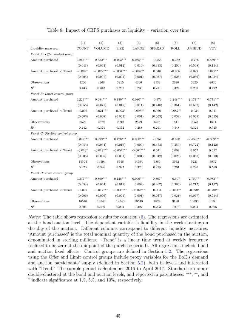
Table 8: Impact of CBPS purchases on liquidity – variation over time

(1) (2) (3) (4) (5) (6) (7) (8)

Liquidity measure: COUNT VOLUME SIZE LARGE SPREAD ROLL AMIHUD VOV

Panel A: Offer control group

Amount purchased 0.266∗∗∗ 0.682∗∗∗ 0.103∗∗∗ 0.085∗∗∗ -0.556 -0.332 -0.776 -0.569∗∗∗

(0.043) (0.063) (0.012) (0.010) (0.335) (0.200) (0.508) (0.114)

Amount purchased × Trend -0.009∗ -0.022∗∗∗ -0.004∗∗∗ -0.002∗∗ 0.048 -0.005 0.029 0.029∗∗

(0.005) (0.007) (0.001) (0.001) (0.037) (0.023) (0.059) (0.014)

Observations 4266 4266 3915 4266 2539 2620 3320 2620

R2 0.433 0.313 0.287 0.239 0.211 0.324 0.280 0.492

Panel B: Limit control group

Amount purchased 0.229∗∗∗ 0.694∗∗∗ 0.130∗∗∗ 0.080∗∗∗ -0.573 -1.248∗∗∗ -2.171∗∗∗ -0.771∗∗∗

(0.055) (0.071) (0.016) (0.011) (0.448) (0.351) (0.567) (0.142)

Amount purchased × Trend -0.006 -0.021∗∗∗ -0.003∗ -0.003∗∗ 0.056 -0.082∗∗ -0.034 0.011

(0.006) (0.008) (0.002) (0.001) (0.053) (0.039) (0.069) (0.015)

Observations 2579 2579 2399 2579 1575 1611 2052 1611

R2 0.442 0.371 0.372 0.288 0.261 0.348 0.321 0.545

Panel C: Sterling control group

Amount purchased 0.342∗∗∗ 0.899∗∗∗ 0.128∗∗∗ 0.098∗∗∗ -0.757 -0.528 -2.488∗∗∗ -0.889∗∗∗

(0.053) (0.064) (0.019) (0.009) (0.473) (0.359) (0.722) (0.122)

Amount purchased × Trend -0.010∗ -0.018∗∗∗ -0.004∗∗∗ -0.002∗∗∗ 0.041 0.002 0.057 0.012

(0.005) (0.005) (0.001) (0.001) (0.042) (0.025) (0.058) (0.010)

Observations 14594 14594 6546 14594 3880 3932 5221 3932

R2 0.623 0.396 0.327 0.320 0.225 0.291 0.280 0.560

Panel D: Euro control group

Amount purchased 0.347∗∗∗ 0.899∗∗∗ 0.128∗∗∗ 0.099∗∗∗ -0.867∗ -0.607 -2.760∗∗∗ -0.983∗∗∗

(0.054) (0.064) (0.019) (0.009) (0.467) (0.366) (0.717) (0.157)

Amount purchased × Trend -0.009 -0.017∗∗∗ -0.003∗∗∗ -0.002∗∗∗ 0.004 -0.044∗∗ -0.099∗ -0.030∗∗

(0.006) (0.006) (0.001) (0.001) (0.037) (0.021) (0.057) (0.014)

Observations 16540 16540 12240 16540 7824 9190 10096 9190

R2 0.604 0.469 0.294 0.397 0.203 0.275 0.294 0.506

Notes: The table shows regression results for equation (6). The regressions are estimatedat the bond-auction level. The dependent variable is liquidity in the week starting onthe day of the auction. Different columns correspond to different liquidity measures.‘Amount purchased’ is the total nominal quantity of the bond purchased in the auction,denominated in sterling millions. ‘Trend’ is a linear time trend at weekly frequency(defined to be zero at the midpoint of the purchase period). All regressions include bondand auction fixed effects. Control groups are defined in Section 5.2. The regressionsusing the Offer and Limit control groups include proxy variables for the BoE’s demandand auction participants’ supply (defined in Section 5.2), both in levels and interactedwith ‘Trend.’ The sample period is September 2016 to April 2017. Standard errors aredouble-clustered at the bond and auction levels, and reported in parentheses. ∗∗∗, ∗∗, and∗ indicate significance at 1%, 5%, and 10%, respectively.

45

Table 9: Stock effects of CBPS on liquidity

(1) (2) (3) (4) (5) (6) (7) (8)

Liquidity measure: COUNT VOLUME SIZE LARGE SPREAD ROLL AMIHUD VOV

Panel A: Eligible control group

Amount purchased 0.006 -0.038 0.001 -0.005 0.228 0.119 -0.572 -0.042

(0.035) (0.034) (0.011) (0.005) (0.474) (0.495) (0.632) (0.256)

Observations 311 311 183 311 41 56 94 56

R2 0.091 0.063 0.122 0.078 0.537 0.311 0.254 0.195

Panel B: Sterling control group

Amount purchased -0.005 -0.067∗∗ -0.002 -0.009∗∗ 0.369 0.092 -0.873∗ 0.035

(0.022) (0.026) (0.007) (0.004) (0.325) (0.257) (0.477) (0.157)

Observations 493 493 279 493 83 88 158 88

R2 0.092 0.074 0.095 0.082 0.239 0.214 0.136 0.144

Notes: The table shows regression results for equation (7). The regressions are estimatedat the bond level. The dependent variable is the change in liquidity from the week be-fore the CBPS was announced (25 – 29 July 2016) to the week after purchases werecompleted (1 – 5 May 2017). Different columns correspond to different liquidity mea-sures. ‘Amount purchased’ is the total quantity of the bond purchased by the CBPS overthe entire purchase period, denominated in sterling millions. All regressions include thefollowing bond-level controls measured before the announcement: amount outstanding,credit rating, residual maturity, residual maturity squared, industry fixed effects, yieldspread to the reference gilt, and amount outstanding of gilts with a similar residual ma-turity (within two years). The regressions also include the following bond-level controlscomputed over the duration of the scheme: change in credit rating, change in amountoutstanding of gilts with a similar residual maturity, and BoE QE purchases of gilts witha similar maturity. Control groups are defined in Section 6. Standard errors are robustto heteroskedasticity and reported in parentheses. ∗∗∗, ∗∗, and ∗ indicate significance at1%, 5%, and 10%, respectively.

46

A Definitions of liquidity measures

We compute eight liquidity measures using the transaction-level Zen dataset. All measures

are computed at the level of individual bonds, and at weekly frequency.

COUNT Number of trades within the week.

VOLUME Total trading volume within the week, denominated in £mn.

SIZE Average trade size, denominated in £mn.

LARGE Number of trades with a market value greater than or equal to £2mn, which

is approximately the 90th percentile of the trade size distribution.

SPREAD The effective spread is used by Hong and Warga (2000), among others, as an

estimate of the average bid-ask spread. We compute this measure as the volume-weighted

average price in trades where a dealer is selling to a non-dealer, minus the volume-weighted

average price in trades where a dealer is buying from a non-dealer, divided by the volume-

weighted average price across all trades. The units are basis points. To compute this

measure, we require there to be at least one sell trade and one buy trade within the week.

ROLL Roll (1984) shows that under certain assumptions, the effective bid-ask spread

is equal to two times the square root of the negative of the first-order serial covariance of

returns. For a given bond and a given week, define ri to be the return on the ith trade.

We then compute the Roll measure as

ROLL = 2√

max {0,−cov (ri, ri−1)}.

The units are basis points. We only compute this measure for weeks with at least four

trades.

AMIHUD Amihud (2002) measures liquidity as the ratio of absolute return to trading

volume. This measure is intended to capture the price impact of trading. Following

Dick-Nielsen et al. (2012), we compute the Amihud measure at the level of individual

trades, then average over the trade-level values each week to obtain a measure at weekly

47

frequency. More precisely, for a given bond and a given week, define ri to be the return

and Qi to be the trade size (in £mn) of the ith trade, and define N to be the number of

trades. We then compute the Amihud measure as

AMIHUD =1

N − 1

N∑i=2

|ri|Qi

.

The units are basis points. We require at least two trades within the week to compute

this measure. We exclude trades smaller than £100k since these can introduce significant

noise.

VOV As an additional measure of price impact, we use the volatility-over-volume mea-

sure of Fong et al. (2017). For a given bond and a given week, let σ2 be the variance

of traded prices and let V be the total trading volume (in £mn). We then compute

volatility-over-volume as

V OV =

√σ2

V.

The units are basis points, and we only compute this measure for weeks with at least four

trades.

48

B Econometric model

We provide an econometric justification for the model in Section 5.2. We suppose that

liquidity is determined by the following equation:

Lbt = αb + µt + βPbt + δᵀZbt + ebt, (8)

where Lbt denotes the liquidity of bond b in period t, Pbt denotes auction purchases, and

Zbt ∈ Rkz is a vector of latent signals about liquidity observed by market participants but

not by the econometrician. We suppose that purchases are determined by demand and

supply factors, so that

Pbt = ab + ct + θᵀXbt + ubt, (9)

where Xbt = (Dᵀbt, S

ᵀbt)

ᵀ ∈ Rkx . The demand and supply factors are themselves driven by

the latent liquidity factor, i.e.,

Xbt = ωb + φt +BZbt + vbt. (10)

Here, αb, µt, ab, ct, ωb, and φt are unobserved bond-specific and time-specific fixed effects

whose relations with other variables are not restricted in any way. Because Zbt is not

observed, the usual difference-in-differences estimator of liquidity Lbt on purchases Pbt

would be inconsistent. The model shares some similarities with Pesaran (2006), except

that the latent factors in our case vary over both bonds and time in an unspecified way.

Suppose that kx = kz = k and that B is of full rank.14 In this case, we may write

Zbt = B−1 (Xbt − vbt − ωb − φt) ,

and hence substituting into (8) we obtain

Lbt = α∗b + γ∗t + βPbt + dᵀXbt + e∗bt, (11)

where e∗bt = ebt−δᵀB−1vbt is a linear combination of ebt and vbt, while α∗b and γ∗t are linear

combinations of the fixed effects from the liquidity equation, the demand equation, and

14This is only for exposition; the argument also works provided rank(B) ≥ kz, i.e., more X than Z.

49

the supply equation. Taking double differences (across b and t), we obtain

Lbt = βPbt + dᵀXbt + e∗bt (12)

Pbt = θᵀXbt + ubt

Xbt = BZbt + vbt,

where Lbt = ∆∆Lbt, Pbt = ∆∆Pbt, etc. Note that e∗bt contains vbt, which is correlated

with Xbt and Pbt, the included variables in (12), the equation of interest. This is like the

classical measurement error problem: since X is an imperfect measure of Z, it usually

leads to biased OLS coefficients (Aigner et al., 1984). However, because P is only driven

by L through Z, this effect can be eliminated, at least as far as the main effect of interest,

using the partitioned regression formula. Let EL(Y |X) denote the best linear predictor

of a random variable Y by a random variable X. We have

EL(Lbt|Xbt) = βEL(Pbt|Xbt) + dᵀXbt + EL(e∗bt|Xbt),

using the linearity of the operator EL(·|·). Subtracting from (12) we obtain

Lbt − EL(Lbt|Xbt) = β(Pbt − EL(Pbt|Xbt)

)+(e∗bt − EL(e∗bt|Xbt)

).

Now, since Pbt−EL(Pbt|Xbt) = ubt, provided EL(ebt, vbt, Xbt|ubt) = 0, the slope of the best

linear predictor of Lbt−EL(Lbt|Xbt) by (Pbt−EL(Pbt|Xbt)) is β. Therefore, for identification

of β it suffices that the following unconditional moment conditions are satisfied:

E (ebt × ubt) = 0 (13)

E (vbt × ubt) = 0 (14)

E (Zbt × ubt) = 0. (15)

In practice, we construct the OLS estimator of β from (12) by the partitioned regression

formula

β = (PᵀMxP)−1PᵀMxL = β + (PᵀMxP)−1PᵀMxE∗,

where P is the nT × 1 vector containing the observations Pbt, L is the nT × 1 vector

50

containing the observations Lbt, while

Mx = InT −X (X ᵀX )−1X ᵀ,

where X is the nT × k matrix containing the observations Xbt. Here, E∗ is the nT × 1

vector containing the observations e∗bt. The partialling out by Mx removes the source of

correlation between the error term in (12) and the included variables.

The moment conditions (13) - (15), along with technical conditions (that are standard

in the difference-in-differences literature) to ensure laws of large numbers and central limit

theorems, guarantee the large sample approximations we use in the paper. The estimates

of d are not particularly meaningful as they involve a number of underlying parameters

(these estimates will be affected by the measurement error bias anyway).

51

C Robustness tests

Table 10: Impact of CBPS purchases on liquidity – without supply and demand controls

(1) (2) (3) (4) (5) (6) (7) (8)

Liquidity measure: COUNT VOLUME SIZE LARGE SPREAD ROLL AMIHUD VOV

Panel A: Offer control group

Amount purchased 0.313∗∗∗ 0.758∗∗∗ 0.118∗∗∗ 0.096∗∗∗ -0.743∗∗ -0.358∗∗ -0.980∗∗∗ -0.679∗∗∗

(0.044) (0.052) (0.013) (0.007) (0.316) (0.165) (0.371) (0.091)

Observations 4266 4266 3915 4266 2539 2620 3320 2620

R2 0.430 0.306 0.278 0.235 0.206 0.322 0.279 0.490

Panel B: Limit control group

Amount purchased 0.345∗∗∗ 0.829∗∗∗ 0.130∗∗∗ 0.102∗∗∗ -0.916∗∗ -0.349 -1.785∗∗∗ -0.693∗∗∗

(0.052) (0.055) (0.016) (0.008) (0.373) (0.242) (0.526) (0.105)

Observations 2579 2579 2399 2579 1575 1611 2052 1611

R2 0.438 0.364 0.363 0.283 0.256 0.341 0.320 0.540

Notes: The table shows regression results for equation (3), excluding the proxy variablesfor supply and demand. The regressions are estimated at the bond-auction level. Thedependent variable is liquidity in the week starting on the day of the auction. Differ-ent columns correspond to different liquidity measures. ‘Amount purchased’ is the totalnominal quantity of the bond purchased in the auction, denominated in sterling millions.All regressions include bond and auction fixed effects. Control groups are defined inSection 5.2. The sample period is September 2016 to April 2017. Standard errors aredouble-clustered at the bond and auction levels, and reported in parentheses. ∗∗∗, ∗∗, and∗ indicate significance at 1%, 5%, and 10%, respectively.

52

Table 11: Impact of CBPS purchases on liquidity – scaled purchases

(1) (2) (3) (4) (5) (6) (7) (8)

Liquidity measure: COUNT VOLUME SIZE LARGE SPREAD ROLL AMIHUD VOV

Panel A: Offer control group

Amount purchased 92.3∗∗∗ 250.3∗∗∗ 49.4∗∗∗ 30.1∗∗∗ -369.9∗∗∗ -178.2∗ -358.1∗∗ -317.1∗∗∗

(17.0) (22.8) (6.1) (3.3) (134.2) (97.6) (166.1) (45.9)

Observations 4266 4266 3915 4266 2539 2620 3320 2620

R2 0.429 0.300 0.293 0.230 0.206 0.323 0.280 0.491

Panel B: Limit control group

Amount purchased 66.3∗∗∗ 235.5∗∗∗ 57.5∗∗∗ 26.3∗∗∗ -272.5 -263.7∗ -776.6∗∗∗ -342.3∗∗∗

(21.2) (25.3) (7.4) (3.5) (179.3) (138.3) (223.7) (56.2)

Observations 2579 2579 2399 2579 1575 1611 2052 1611

R2 0.438 0.355 0.376 0.278 0.257 0.342 0.321 0.542

Panel C: Sterling control group

Amount purchased 119.3∗∗∗ 334.4∗∗∗ 59.6∗∗∗ 36.7∗∗∗ -358.3 -307.4∗ -1232.1∗∗∗ -446.8∗∗∗

(20.0) (27.4) (8.8) (3.5) (217.7) (169.7) (288.1) (72.2)

Observations 14594 14594 6546 14594 3880 3932 5221 3932

R2 0.622 0.391 0.327 0.317 0.224 0.291 0.281 0.560

Panel D: Euro control group

Amount purchased 120.2∗∗∗ 334.1∗∗∗ 58.9∗∗∗ 37.1∗∗∗ -320.8 -244.1 -1088.8∗∗∗ -396.4∗∗∗

(19.8) (27.0) (8.8) (3.5) (209.7) (176.1) (284.3) (79.5)

Observations 16540 16540 12240 16540 7824 9190 10096 9190

R2 0.604 0.467 0.293 0.396 0.203 0.275 0.294 0.506

Notes: The table shows regression results for equation (3). The regressions are estimatedat the bond-auction level. The dependent variable is liquidity in the week starting onthe day of the auction. Different columns correspond to different liquidity measures.‘Amount purchased’ is the total nominal quantity of the bond purchased in the auction,divided by the nominal amount of the bond outstanding. All regressions include bondand auction fixed effects. Control groups are defined in Section 5.2. The regressions usingthe Offer and Limit control groups include proxy variables for the BoE’s demand andauction participants’ supply (defined in Section 5.2). The sample period is September2016 to April 2017. Standard errors are double-clustered at the bond and auction levels,and reported in parentheses. ∗∗∗, ∗∗, and ∗ indicate significance at 1%, 5%, and 10%,respectively.

53

Table 12: Impact of CBPS purchases on liquidity – common correlated effects

(1) (2) (3) (4) (5) (6) (7) (8)

Liquidity measure: COUNT VOLUME SIZE LARGE SPREAD ROLL AMIHUD VOV

Panel A: Offer control group

Amount purchased 0.291∗∗∗ 0.724∗∗∗ 0.094∗∗∗ 0.083∗∗∗ -0.924∗∗ -0.518 -1.009 -0.576∗∗∗

(0.044) (0.061) (0.009) (0.010) (0.410) (0.358) (0.684) (0.163)

Observations 4275 4275 3929 4275 2533 2584 3333 2584

Panel B: Limit control group

Amount purchased 0.310∗∗∗ 0.880∗∗∗ 0.102∗∗∗ 0.101∗∗∗ -0.537 -1.124∗ -2.672∗∗ -0.672∗∗∗

(0.080) (0.104) (0.016) (0.017) (0.724) (0.618) (1.181) (0.258)

Observations 2601 2601 2425 2601 1588 1611 2076 1611

Panel C: Sterling control group

Amount purchased 0.455∗∗∗ 0.964∗∗∗ 0.140∗∗∗ 0.097∗∗∗ -0.495 -0.268 -2.141∗∗ -0.559∗∗

(0.042) (0.057) (0.013) (0.009) (0.520) (0.504) (1.018) (0.228)

Observations 14596 14596 6526 14596 3742 3836 5140 3836

Panel D: Euro control group

Amount purchased 0.387∗∗∗ 0.934∗∗∗ 0.134∗∗∗ 0.097∗∗∗ -0.962∗∗ -0.569 -2.238∗∗∗ -0.598∗∗∗

(0.085) (0.085) (0.009) (0.012) (0.398) (0.360) (0.654) (0.167)

Observations 16534 16534 12229 16534 7765 9137 10052 9137

Notes: The table shows regression results for equation (3). The regressions are estimatedat the bond-auction level using the pooled common correlated effects (CCE) estimator ofPesaran (2006). The dependent variable is liquidity in the week starting on the day ofthe auction. Different columns correspond to different liquidity measures. ‘Amount pur-chased’ is the total nominal quantity of the bond purchased in the auction, denominatedin sterling millions. All regressions include bond and auction fixed effects. Control groupsare defined in Section 5.2. The regressions using the Offer and Limit control groups in-clude proxy variables for the BoE’s demand and auction participants’ supply (defined inSection 5.2). The sample period is September 2016 to April 2017. Standard errors aredouble-clustered at the bond and auction levels, and reported in parentheses. ∗∗∗, ∗∗, and∗ indicate significance at 1%, 5%, and 10%, respectively.

54