Bank of EnglandCentre for Central Banking Studies

CEMLA 2013

Value at Risk.David G. Barr∗

November 21, 2013

∗Any views expressed are those of the author and not necessarily those of the Bank of England.

1

Contents

1 Risk and volatility. 31.1 Illustrating a problem with volatility. . . . . . . . . . . . . . . . . . . . . . . . . . . . . . . . . . . . . . 3

2 Value at risk: Introduction. 72.1 VaR for a simple discrete distribution. . . . . . . . . . . . . . . . . . . . . . . . . . . . . . . . . . . . . 72.2 VaR and the Normal distribution. . . . . . . . . . . . . . . . . . . . . . . . . . . . . . . . . . . . . . . 8

2.2.1 Revision of hypothesis tests. . . . . . . . . . . . . . . . . . . . . . . . . . . . . . . . . . . . . . . 82.2.2 From hypothesis tests to VaR. . . . . . . . . . . . . . . . . . . . . . . . . . . . . . . . . . . . . 102.2.3 A general formula for Normally distributed returns. . . . . . . . . . . . . . . . . . . . . . . . . 11

2.3 VaR again, in words this time. . . . . . . . . . . . . . . . . . . . . . . . . . . . . . . . . . . . . . . . . 13

3 Value at Risk: An example. 143.1 SP500: Daily returns. . . . . . . . . . . . . . . . . . . . . . . . . . . . . . . . . . . . . . . . . . . . . . 143.2 Longer time periods. . . . . . . . . . . . . . . . . . . . . . . . . . . . . . . . . . . . . . . . . . . . . . . 15

4 Don’t forget.... 16

5 Problems with VaR. 175.1 When the VaR represents a profit rather than a loss. . . . . . . . . . . . . . . . . . . . . . . . . . . . . 175.2 VaR is ‘optimistic’. . . . . . . . . . . . . . . . . . . . . . . . . . . . . . . . . . . . . . . . . . . . . . . . 175.3 VaR may violate the basic rule of diversification. . . . . . . . . . . . . . . . . . . . . . . . . . . . . . . 18

6 An alternative to VaR: Expected shortfall (ES). 206.1 Definition of expected shortfall. . . . . . . . . . . . . . . . . . . . . . . . . . . . . . . . . . . . . . . . . 20

6.1.1 ES for a Normal distribution. . . . . . . . . . . . . . . . . . . . . . . . . . . . . . . . . . . . . . 216.2 The SP500 example again. . . . . . . . . . . . . . . . . . . . . . . . . . . . . . . . . . . . . . . . . . . . 23

A Volatility over several periods. 24

2

1. Risk and volatility.

• Can we sum up the riskiness of an asset, or portfolio, in a single-valued

measure?

– Obtaining a single-value measure is important if we want to rank

assets by risk.

• Traditionally this was achieved using volatility i.e. standard deviation.

• While volatility is still used, as a single summary measure of risk it

has some deficiencies:

– It’s symmetric i.e. upside and downside risks are measured in the

same way.

– It does not deal well with heavy-tailed distributions.

∗ ‘Heavy’ being defined in relation to the Normal distribution.

1.1. Illustrating a problem with volatility.

• The following time series of asset returns all have mean zero, and

volatility 1.

• But they come from three different distributions: N(0,1), t(3) and a

‘jump distribution’.

– The variance of a t(n) is n/(n − 2), so we divide the t(3) data by√3.

3

Figure 1: N(0,1) and t(3)/√

3 variables.

4

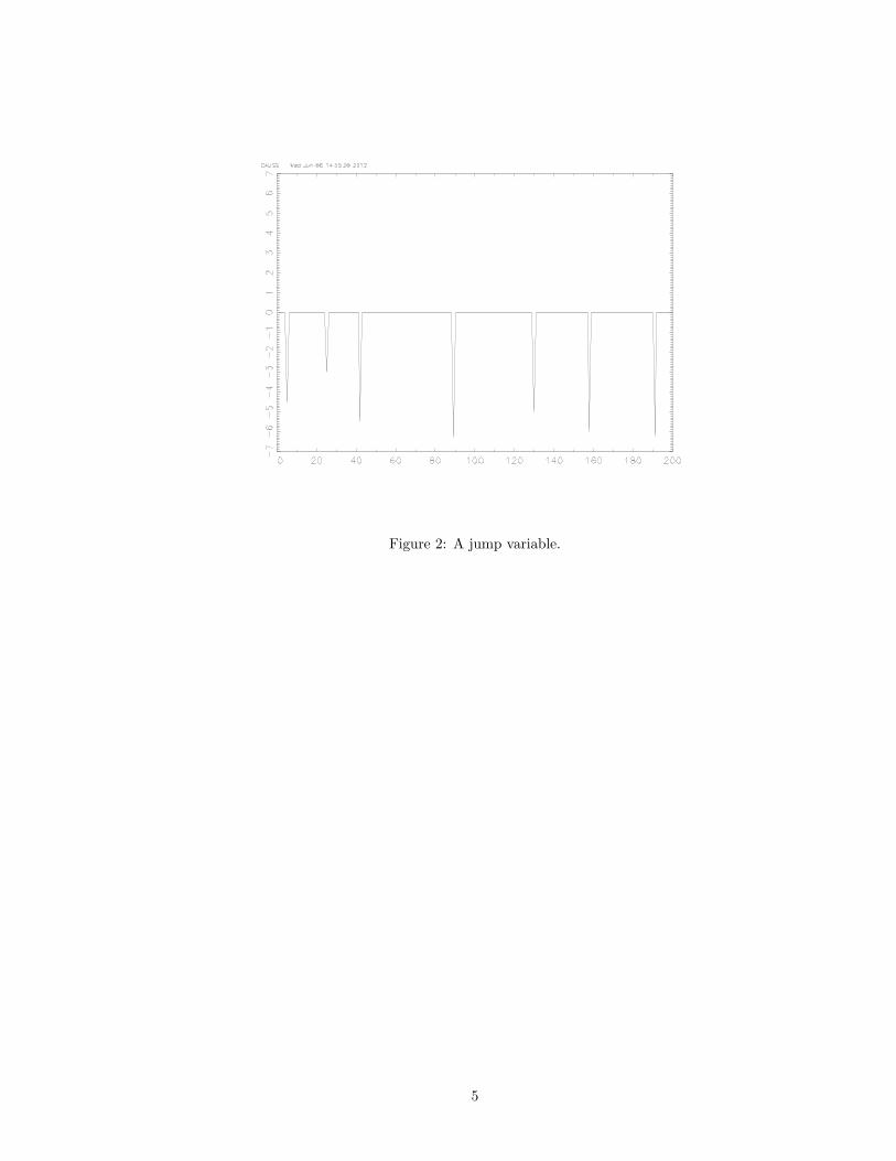
Figure 2: A jump variable.

5

• Which is the most risky for a bank that will go bankrupt if the loss

hits -4%?

• Value at Risk (VaR) offers an alternative, also single-value, measure

of risk.

6

2. Value at risk: Introduction.

• A popular, but imperfect, alternative to volatility.

• Invented by JPMorgan and propagated in ‘RiskMetrics’,

– VaR is not symmetric (it looks only at losses).

– It treats heavy tails sensibly, up to a point.

• VaR analysis provides values for x and k in the following statement:

“We can be x% confident that we will not lose more than

$k.”

• But, before we can make use of the VaR measure we need to decide

on:

1. The length of the time period over which the risk is of concern.

2. The probability distribution of the risky variable (asset price etc).

– N.B. The VaR approach does not require Normality.

– We will see later that we don’t need the whole of the distribution.

3. A ‘confidence level’ i.e. x in the above statement.

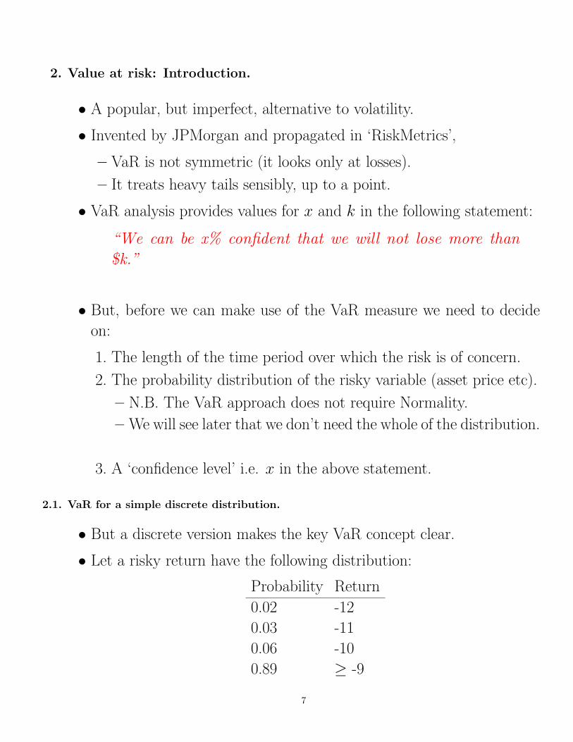
2.1. VaR for a simple discrete distribution.

• But a discrete version makes the key VaR concept clear.

• Let a risky return have the following distribution:

Probability Return

0.02 -12

0.03 -11

0.06 -10

0.89 ≥ -9

7

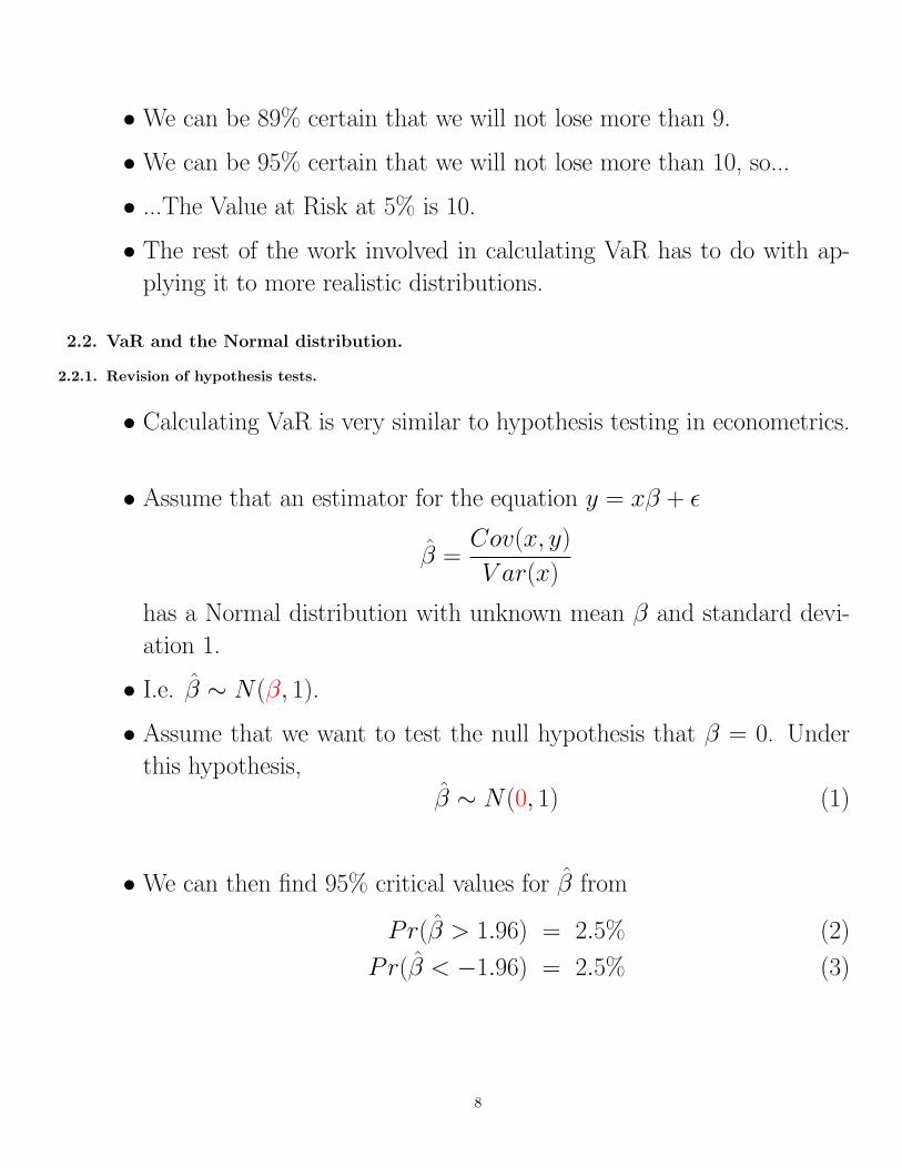
• We can be 89% certain that we will not lose more than 9.

• We can be 95% certain that we will not lose more than 10, so...

• ...The Value at Risk at 5% is 10.

• The rest of the work involved in calculating VaR has to do with ap-

plying it to more realistic distributions.

2.2. VaR and the Normal distribution.

2.2.1. Revision of hypothesis tests.

• Calculating VaR is very similar to hypothesis testing in econometrics.

• Assume that an estimator for the equation y = xβ + ε

β̂ =Cov(x, y)

V ar(x)

has a Normal distribution with unknown mean β and standard devi-

ation 1.

• I.e. β̂ ∼ N(β, 1).

• Assume that we want to test the null hypothesis that β = 0. Under

this hypothesis,

β̂ ∼ N(0, 1) (1)

• We can then find 95% critical values for β̂ from

Pr(β̂ > 1.96) = 2.5% (2)

Pr(β̂ < −1.96) = 2.5% (3)

8

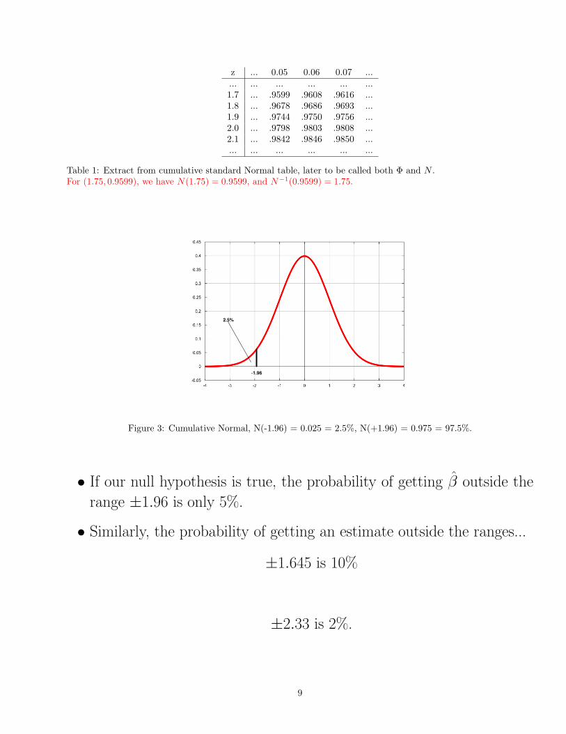
z ... 0.05 0.06 0.07 ...... ... ... ... ... ...1.7 ... .9599 .9608 .9616 ...1.8 ... .9678 .9686 .9693 ...1.9 ... .9744 .9750 .9756 ...2.0 ... .9798 .9803 .9808 ...2.1 ... .9842 .9846 .9850 ...... ... ... ... ... ...

Table 1: Extract from cumulative standard Normal table, later to be called both Φ and N .For (1.75, 0.9599), we have N(1.75) = 0.9599, and N−1(0.9599) = 1.75.

2.5%

-1.96

Figure 3: Cumulative Normal, N(-1.96) = 0.025 = 2.5%, N(+1.96) = 0.975 = 97.5%.

• If our null hypothesis is true, the probability of getting β̂ outside the

range ±1.96 is only 5%.

• Similarly, the probability of getting an estimate outside the ranges...

±1.645 is 10%

±2.33 is 2%.

9

±2.57 is 1%.

• So if we get β̂ = 2.00:

– we can be 95% confident that the null hypothesis is wrong but...

– ...we cannot be 99% confident that it is wrong.

2.2.2. From hypothesis tests to VaR.

• We now move to considering financial risks instead of econometric

estimates.

• We start by looking at the risk of a financial asset.

• We continue to use the Normal distribution but:

– The Normal distribution extend to minus infinity.

– Very few assets have returns that can get this bad (a short call

option being an exception).

– E.g. an equity’s percentage return will lie in the range -100% to

+∞.

• From the examples we know that the probability of getting β̂ lower

than −1.645 is 5%.

• Now let β be the (unknown) future dollar return on an asset, let it

have distribution β ∼ N(0, 1), and let β̂ be the realisation of that

change.

• We get the probability that the asset price will fall by 1.645 or more

as 5%.

• This is the value at risk at 5% i.e.

VaR(5%) = 1.645.

10

and, similarly,

VaR(1%) = 2.33.

• Note that for these examples:

– We have assumed σ = 1.

– These numerical VaR results are for a N(0,1) distributed asset re-

turn, and not for any other distribution.

2.2.3. A general formula for Normally distributed returns.

• For the more general distribution r ∼ N(µ, σ), we transform r into

the standard normal variate z where

z =r − µ

σ∼ N(0, 1) (4)

so that we can continue to use the above N(0, 1) table.

• For the lhs of the distribution r ∼ N(µ, σ) we have,

Pr

(r − µ

σ< −1.645

)= 0.05 (5)

• We find the critical value r5% as

r5% − µ

σ= −1.645 (6)

⇒ r5% = µ− 1.645σ (7)

11

5%

-1.645

z = (r - mu)/sigma

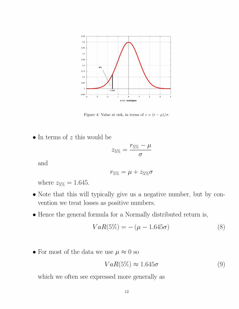
Figure 4: Value at risk, in terms of z = (r − µ)/σ.

• In terms of z this would be

z5% =r5% − µ

σ

and

r5% = µ + z5%σ

where z5% = 1.645.

• Note that this will typically give us a negative number, but by con-

vention we treat losses as positive numbers.

• Hence the general formula for a Normally distributed return is,

V aR(5%) = − (µ− 1.645σ) (8)

• For most of the data we use µ ≈ 0 so

V aR(5%) ≈ 1.645σ (9)

which we often see expressed more generally as

12

V aR(S%) ≈ N−1(S%)σ (10)

where N−1(S%) can be read off the standard Normal tables.

2.3. VaR again, in words this time.

• Given a distribution we can we find numbers such that we can state

that:

– ‘We can be x% confident that we will not lose more than $k.’

– Or, ‘The probability that we will not lose more than $k is x%.’

• VaR allows us to rewrite this as:

– ‘We can be 95% certain that we will not lose more than $VaR(5%).’

where VaR(5%) is a number to be calculated using the chosen distri-

bution.

• Or, ‘We can be 99% certain that we will not lose more than $VaR(1%).’

• And, more generally,

– ‘We can be p% certain that we will not lose more than $VaR(100-

p)%).’

13

3. Value at Risk: An example.

3.1. SP500: Daily returns.

• The estimated logNormal distribution for SP500 daily returns is

N(0.0295%, 0.1399%).

• I.e.

ln(1 + r) ∼ N(0.000295, 0.001399)

• Find the 5% VaR for a $1m investment in the index.

• The 5% ‘critical value’ for ln(1 + r), is found from:

ln(1 + r)5% = − (µ− 1.645σ) (11)

= − (0.000295− 1.645× 0.001399) (12)

= 0.002006 (13)

• The equivalent return in natural units is found as:

1 + r5% = eln(1+r)5% (14)

r5% = eln(1+r)5% − 1 (15)

= e0.002006 − 1 (16)

= 1.002008− 1 (17)

= 0.002008 (18)

= 0.2008% (19)

• So we can be 95% certain that we will not lose more than $2008 in any

one day.

• The 5% VaR here is referred to in some texts as its complement i.e.

as a 95% VaR.

• The time period is important. Here the data are for daily returns, and

are used to construct daily moments for the probability distribution.

14

• As a result, we get only a 1-day VaR.

3.2. Longer time periods.

• We may have data only for daily returns.

• If we want to calculate a 5-day VaR we need the moments for 5-day

returns.

• If the daily dollar returns are Normally distributed (µ, σ) and the

realisations are independent of each other we can scale the daily

mean and standard deviation up to 5 days as:

µ5 = 5× µ1 (20)

σ5 =√

5× σ1 (21)

• We often approximate the mean by zero, in which case we get,

V aR(n days) ≈√

n× V aR(1 day) (22)

• So for the approximate value at risk over 30 days we get

V aR30(5%) ≈√

30× V aR1(5%) = 5.48× $2008 = $11004 (23)

• Adjusting the VaR for other distributions is more complicated than

this.

• Note that we have assumed the returns and in dollar terms here. If

we have proportionate returns, and these are logNormally distributed,

the equivalent scaling factor is e√

30 instead of√

30.

15

4. Don’t forget....

For Normally distributed returns, VaR(1%) is the return that is 2.33

standard deviations below the mean, multiplied by minus one.

and, more generally,

V aR(S%) = −σΦ(S%) for µ = 0 (24)

where Φ(S%) is the inverse Normal distribution function (the one in the

tables at the back of most statistics textbooks) and S% is typically 1% or

5% (as opposed to 99% or 95% as in Hull’s Risk Management text.)

16

5. Problems with VaR.

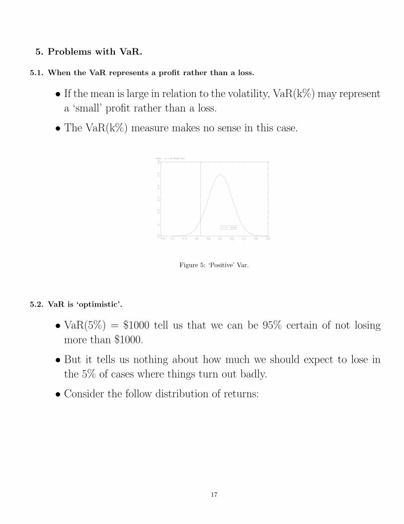
5.1. When the VaR represents a profit rather than a loss.

• If the mean is large in relation to the volatility, VaR(k%) may represent

a ‘small’ profit rather than a loss.

• The VaR(k%) measure makes no sense in this case.

Figure 5: ‘Positive’ Var.

5.2. VaR is ‘optimistic’.

• VaR(5%) = $1000 tell us that we can be 95% certain of not losing

more than $1000.

• But it tells us nothing about how much we should expect to lose in

the 5% of cases where things turn out badly.

• Consider the follow distribution of returns:

17

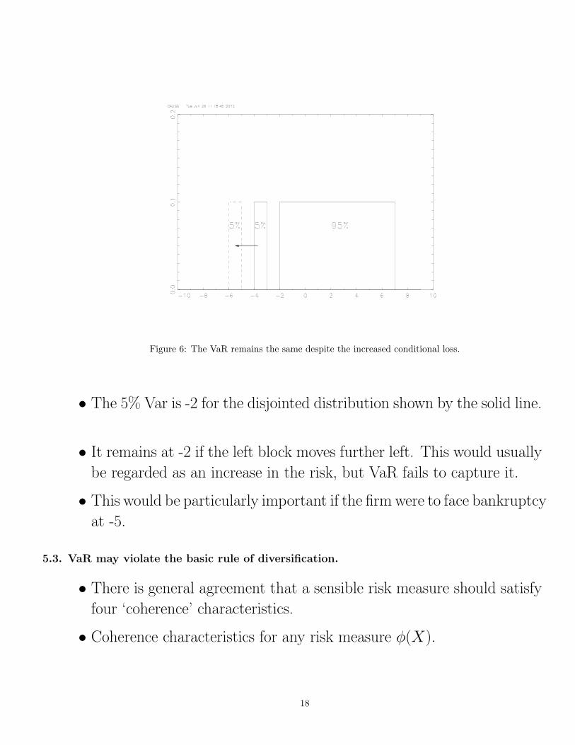
Figure 6: The VaR remains the same despite the increased conditional loss.

• The 5% Var is -2 for the disjointed distribution shown by the solid line.

• It remains at -2 if the left block moves further left. This would usually

be regarded as an increase in the risk, but VaR fails to capture it.

• This would be particularly important if the firm were to face bankruptcy

at -5.

5.3. VaR may violate the basic rule of diversification.

• There is general agreement that a sensible risk measure should satisfy

four ‘coherence’ characteristics.

• Coherence characteristics for any risk measure φ(X).

18

1. Monotonicity: If we have two asset returns, X and Y , and if in

all realisations X ≤ Y , then φ(X) ≥ φ(Y ).

2. Subadditivity: A diversified portfolio cannot be more risky than

its constituent assets, so φ(X + Y ) ≤ φ(X) + φ(Y ).

3. Homogeneity: If the portfolio value increases by n times then

so does the risk: φ(nX) = nφ(X).

4. Translation invariance: If we add $c of riskless cash to the

portfolio the risk should fall i.e. φ(X + c) = φ(X)− c.

• The second of these refers to portfolio diversification.

• VaR can fail to exhibit subadditivity if the tails of the distribution are

heavy enough (tail index > 2 - we look at tail indices in the Extreme

Value Theory session).

19

6. An alternative to VaR: Expected shortfall (ES).

6.1. Definition of expected shortfall.

• ES is the expected size of the loss given that the VaR has been exceeded

i.e.

ES(p) = −E[X‖X ≤ V aR(p)] > 0 (25)

• For the discrete example we had earlier,

Probability Return

0.02 -12

0.03 -11

0.06 -10

0.89 ≥ -9

if V aR(5%) = 10 is exceeded, there are only two possible losses, -11

and -12.

• To get the expected value of the loss we have to scale the probabilities

to sum to 1, without changing their relative values.

• We do this as follows:

p′−12 =p−12

p−11 + p−12(26)

=0.02

0.02 + 0.03(27)

= 0.4 (28)

p′−11 =p−11

p−11 + p−12(29)

=0.03

0.02 + 0.03(30)

= 0.6 (31)

20

• Note that the denominator 0.02 + 0.03 = 0.05 = 5% is the VaR that

we are basing the ES on.

• We then get the expected loss as:

ES = −[0.4×−12 + 0.6×−11] (32)

= 11.4 (33)

• As with VaR, the rest of the ES work deals with how to calculate ES

for more realistic distributions.

6.1.1. ES for a Normal distribution.

• For standard Normal (N(0,1)) Danielsson p87 gives the following VaR

and ES values for N(0, 1) profit/loss distribution:

p 0.5 0.1 0.05 0.025 0.01 0.0001

VaR(p) 0 1.282 1.645 1.960 2.326 3.090

ES(p) 0.798 1.755 2.093 2.338 2.665 3.367

• For example, for p = 0.05, we get V aR(5%) = 1.645 i.e. we can be

95% certain of not losing more than 1.645.

• If, however, we are told that this loss has been exceeded, we know that

the actual return must lie in the range (−∞,−1.645).

• Then the expected loss, given this information, is $2.093.

• Other things to note about ES:

– ES always satisfies the diversification rule.

– If the distribution of returns is Normal, then as p → 0 so V aR(p) →ES(p). Look for this in the table above.

21

– The general formula for ES given rates of return distributed N(µ, σ),

is

ES(p) = −(

µ− σ

(φ(N−1(p))

p

))(34)

where φ(x) is the Normal density function, and Ψ(x) is the Normal

cumulative distribution function.

• So, for example, for µ = 0, σ = 1 and p = 0.01,

ES(0.01) = −(

µ− σ

(φ(N−1(0.01)

0.01

))(35)

=

(φ(−2.3263)

0.01

)(36)

=

(0.0267

0.01

)(37)

= 2.6652 (38)

22

6.2. The SP500 example again.

• The SP500 estimated parameters were µ̂ = 0.0295%, σ̂ = 0.1399%

• To keep things simple we assume, incorrectly, that the returns are

Normally distributed (we assumed them to be log Normal earlier).

• We get,

V aR(0.05) = −(µ− σN−1(0.05)) (39)

= −0.0295 + 0.1399× 1.645 (40)

= −0.0295 + 0.2301 (41)

= 0.2006 (42)

(0.2008 when we assumed log Normality) and,

23

ES(0.05) = −(

µ− σ

(φ(N−1(0.05)

0.05

))(43)

= −0.0295 + 0.1399

(φ(−1.645)

0.05

)(44)

= −0.0295 + 0.1399

(0.1031

0.05

)(45)

= −0.0295 + 0.1399× 2.0699 (46)

= −0.0295 + 0.2885 (47)

= 0.259 (48)

A. Volatility over several periods.

• We are used to seeing the following relationship between variances for

multiples of random variables:

V (nx) = n2V (x) (49)

or,

σ5days = 5σ1day (50)

so why do we have

σ5days =√

5σ1day (51)

in equation (21)?

• This can be demonstrated in a 2-day example.

• Let the random return for the first day be x1, and for the second x2,

then

V (x1 + x2) = V (x1) + V (x2) + Cov(x1, x2) (52)

24

• We assumed for (21) that the returns on the 2 days are independently

distributed, so Cov(x1, x2) = 0.

• We also assumed that they have the same variance, call it V (x).

• Hence

V (x1 + x2) = V (x1) + V (x2) = 2V (x) (53)

and

σx1+x2 =√

2V (x) = σx

√2 (54)

.

• In equation (49) above we are multiplying a single realisation by n,

not adding two different realisations from the same distribution.

• The algebra behind (49), works as follows,

V (2x) = V (x + x) (55)

= V (x) + V (x) + 2Cov(x, x) (56)

= V (x) + V (x) + 2V (x) (57)

= 4V (x) (58)

• So it all revolves around the Cov term, and whether or not it equals

zero.

25