bank loan components and the time ... - wouter den haan loan components and the time-varying...

Bank Loan Components and the Time-Varying E¤ects of

Monetary Policy Shocks

Wouter J. Den Haan

University of Amsterdam and CEPR

Steven W. Sumner

University of San Diego

Guy M. Yamashiro

California State University, Long Beach�

March 22, 2010

Abstract

The impulse response functions (IRF) of an aggregate variable is time varying if

the IRFs of its components are di¤erent from each other and the relative magnitudes

of the components are not constant� two conditions likely to be true in practice. We

model the behavior of loan components and document that the induced time variation

for total loans is substantial, which helps to explain why studies describing total loans

have had such a hard time �nding a robust response of total bank loans to a monetary

tightening.

Keywords: Small and large banks, VAR, impulse response functions

JEL Classi�cation: E40

�Den Haan: Amsterdam School of Economics, University of Amsterdam, Roetersstraat 11, 1018 WB

Amsterdam, The Netherlands, [email protected]. Sumner: Department of Economics, University of San

Diego, San Diego, USA, [email protected]. Yamashiro: Department of Economics, California State

University, Long Beach, USA, [email protected]. The authors would like to thank Anil Kashyap, Frank

Smets, and William Watkins for useful comments. Den Haan thanks the Netherlands Organisation for

Scienti�c Research (NWO) for �nancial support.

1 Introduction

Relationships between key macroeconomic variables are often changing over time. For

example, several articles have pointed out that responses of variables like GDP and the

unemployment rate to (structural) shocks are di¤erent when they are estimated using

post-1980 data, than when they are estimated using pre-1980 data. During the coming

years, much research is likely to be devoted to the question whether, given the recent

�nancial crisis, a new era has started in which responses are again di¤erent.

The standard procedure to uncover the responses of economic variables to shocks is

to estimate a structural vector autoregressive system (VAR) and to calculate the impulse

response functions (IRFs). To deal with time-varying responses in VARs one could simply

split the sample or use rather complex Bayesian methodologies that allow all parameters

of the VAR to change over time.

It is important to understand why responses can change over time. Not only does

this help us to comprehend the underlying economics better, it also sheds light on what

econometric technique to use to deal with the time-varying aspects of the problem. In

this paper, we emphasize that the percentage response of an aggregate variable will only

be constant through time if the percentage responses of its components and the relative

magnitudes of the components have stayed the same.1 Even if the responses of the compo-

nents are not time varying, then the response of the aggregate variable will depend on the

relative magnitudes of the components when the shock occurs, and, thus, be time varying

if the relative importance of the components is time varying. In other words, the response

of the aggregate variable depends on the initial conditions of the components. If the rel-

ative size of the components is cyclical, then the response of the aggregate variable will

itself be cyclical. If there is a low-frequency change in the relative size of the components,

then there will be a gradual change in the response of the aggregate variable.

The consequence of using aggregate data for time-varying IRFs has received little

attention in the literature, even though the use of aggregate data is widespread. To

illustrate the quantitative importance of the time variation induced by aggregation, we

1As discussed in more detail in the next section, we focus on the commonly used log-linear speci�cation.

1

model the behavior of the loan components and then show that the implied time-variation

in the response of total loans is substantial. The three loan components are commercial

and industrial (C&I) loans, consumer loans, and mortgages.

There are three reasons why loans are interesting to consider. First, Den Haan, Sum-

ner, and Yamashiro (2007, 2009) document that the responses of these three loan compo-

nents following a monetary tightening are quite di¤erent. In particular, whereas consumer

loans and mortgages decrease following a monetary downturn, C&I loans increase. All

responses are economically and statistically signi�cant. This is found to be the case for

both Canadian and US bank loans and for di¤erent samples. In this paper, we extend the

results of Den Haan, Sumner, and Yamashiro (2007, 2009) and show that this result is

found for both small and large banks.2 In contrast, during a non-monetary downturn the

largest drop is found for C&I loans.3

Second, the relative magnitudes of these loan components have changed a lot. The

share of real estate loans has increased for both small and large banks. For small banks the

counterpart is mainly a reduction in consumer loans and for large banks it is a reduction

in C&I lending.

The two �ndings that the bank loan components move in di¤erent directions and that

their relative magnitude has changed over time suggest that it may not be that easy to

�nd a robust response of total bank loans. In fact, Gertler and Gilchrist (1993) point out

that while conventional wisdom holds that a monetary tightening should be followed by a

reduction in bank lending, it has been surprisingly di¢ cult to �nd convincing time-series

evidence to support this basic prediction of economic theory. The third reason to focus

on bank loans is that it may shed light on this puzzle. That is, the response of total loans

is not robust and a researcher may interpret this as a sign that it is time varying. We

show that the changes in the loan shares themselves predict a substantial variation in the

response of total loans even if the responses of the loan components are not time varying.

2The robustness is remarkable given that Kashyap and Stein (1995) �nd more substantial di¤erences

between the behavior of small banks and large banks in several aspects.3A non-monetary downturn is an economic downturn that is not associated with an increase in the

interest rate.

2

In the econometrics literature, there are many papers that deal with aggregation.4

These papers typically focus on the misspeci�cation of the time-series model with aggregate

variables and the e¢ ciency of the estimation procedure. Moreover, linear frameworks are

typically used.5 The focus of our paper di¤ers from this literature. First, although our

time-series model is very simple, it is nonlinear because the logarithms, not the levels of

the variables, enter the VAR. Recall, that the logarithm of the aggregate variable is not

the sum of the logarithms of the components; it is a nonlinear function of the components.

In addition, we are mainly interested in the implication of this commonly used nonlinear

setup that the impulse response function of an aggregate variable is time varying.6

The rest of this paper is organized as follows. In Section 2, we explain why the impulse

response function of a variable that is the sum of other variables in a log-linear system is

time varying. Section 3 discusses the data used and the empirical methodology. Section

4 reports the results for the bank loan components, and Section 5 documents the time-

varying responses of total loans implied by the estimated VAR with loan components.

Section 6 documents that our reason for time variation, i.e., changing weights, can explain

part of the time variation found in the estimates for total loans obtained using rolling

windows. The last section concludes.

2 Time-varying impulse response functions

In this section, we show that the impulse response functions of aggregate variables in

disaggregated log-linear systems are, in general, time varying.7 In particular, the aggregate

responses depend on the (relative) initial values of the micro components, which are, of

course, stochastic and depend upon the history of shocks. We will see that even the

4See, for example, Granger (1980) and Pesaran, Pierse, and Kumar (1989).5An exception is van Garderen, Lee, and Pesaran (2000).6See Potter (1999) for an overview of non-linear time-series models.7The econometrics literature on the advantages and disadvantages of disaggregated models typically

considers linear systems. In a linear system, the implied impulse response functions of aggregate variables

would not be time varying (unless at least one of the impulse response functions of the components is time

varying). In practice, one typically uses log-linear systems to ensure that the e¤ect of a shock, expressed

as a percentage change, does not depend on the value of the variable.

3

shape and sign of the impulse response functions of aggregate variables can change over

time. It is important to realize that the aggregate responses are time varying even though

the coe¢ cients of the VAR are constant and the impulse response functions of the micro

components are, thus, by construction not time varying.

To provide intuition we discuss a simple example in which we trace the behavior of

an aggregate variable in response to a structural shock. The disaggregated system is as

follows.

ln(z1;t) = �1 ln(z1;t�1) + �1et (1a)

ln(z2;t) = �2 ln(z2;t�1) + �2et (1b)

zt = z1;t + z2;t (1c)

Here z1;t and z2;t are the two micro components that add up to the aggregate variable

zt and et is a white noise structural error term with unit variance.8 We focus on the

responses of zt to changes in the structural shock et.

2.1 Dependence on initial values

To understand why the response of the aggregate variable is, in general, time varying

consider the formula for the k-th period percentage change in zt.9

zt+k � ztzt

=

�z1;tzt

��z1;t+k � z1;t

z1;t

�+

�z2;tzt

��z2;t+k � z2;t

z2;t

�(2)

=

�z1;tzt

� bz1;k + �z2;tzt

� bz2;kThus, the percentage change in zt is a weighted average of the percentage change in z1;t

and the percentage change in z2;t. The percentage changes in z1;t and z2;t, bz1;k and bz2;k,are by construction not time varying, since the laws of motion are linear. In contrast, the

8We assume that j�1j < 1 and j�2j < 1:9Here we use the actual percentage change of zt and pretend that Equations (1a) and (1b) give actual

percentage changes in z1;t and z2;t instead of log changes. The argument is the same for the speci�cation

with logs, but the formula is less transparent.

4

weights, z1;t=zt and z2;t=zt, are time varying, which implies that the percentage change in

zt is also time varying. The only exception to this occurs when the laws of motion for z1;t

and z2;t are identical.

To illustrate the time-varying nature of the impulse response functions of zt, we will

focus on the case where �2 = �2 = 0. Equation (1b) then becomes

ln(z2;t) = 0: (3)

Even in this very simple case, for which zt = z1;t + 1 and the value of z1;t relative to z2;t

is simply the value of z1;t, the impulse response function of zt will vary with the value of

z1;t. To document this dependence we plot, in Figure 1, the response of ln(zt) to a one

standard deviation shock to et for �ve initial values of ln(z1;t). The initial values range

from two times the unconditional standard deviation of ln(z1;t) below the unconditional

mean to two times the unconditional standard deviation above the mean. For low values

of ln (z1;t) the response of zt to a shock is low because the e¤ect on zt is dominated by the

zero e¤ect on z2;t. For high values of ln (z1;t) the response of zt is large because the e¤ect

on zt is dominated by the strong e¤ect on z1;t. Even the shape of the impulse response

function varies with the initial value of z1;t. In response to the shock, the value of z1;t

increases relative to the value of z2;t. When z1;t is large this does not matter much since

the movements of zt are dominated by the behavior of z1;t. Consequently, for high values

of z1;t we get an impulse response function for zt that is similar to the impulse response

function of z1;t. When z1;t is small, however, z1;t increases relative to z2;t, meaning that

changes in z1;t will become more important for movements in zt in the periods following

the shock. The �gure shows that this e¤ect can be so strong that the percentage change

in the aggregate variable is initially increasing even though the percentage change in z1;t

is (by construction) monotonically decreasing.

2.2 E¤ects of the �rst and subsequent shocks

Since the response of the aggregate variable depends upon the relative size of the micro

components, the e¤ect of the �rst shock in et will have a di¤erent e¤ect than subsequent

shocks. For example, consider the case in which z1;t is more responsive to et than z2;t. A

5

subsequent positive shock of equal magnitude, then always has a larger e¤ect. The reason

for this is that a positive shock will increase the relative magnitude of the more sensitive

component, z1;t, and this increase in z1;t causes the e¤ect of a percentage change in z1;t on

zt to increase. We demonstrate this e¤ect by doing the following. First we calculate the

impulse response function of zt using some initial conditions for z1;t. Next we calculate

the impulse response function of zt using, as initial conditions, the values of z1;t observed

in the period after the �rst shock. This second impulse response function, thus, does not

measure the total e¤ect of the two shocks but only the additional e¤ect of the second

shock. Again we focus on the case with �2 = �2 = 0.

In this exercise we use two di¤erent values for z1;t at the time of the �rst shock. In

particular, we consider values of ln(z1;t) that are equal to two standard deviations below

and above the mean. These are the two extremes of the �ve initial values considered

in Figure 1. The results are presented in Figure 2. The �gure shows that when z1;t is

already high relative to z2;t, a further increase in z1;t in response to the �rst shock does not

increase the sensitivity of zt to the shock. Consequently, the e¤ect of the second shock is

only slightly bigger than the e¤ect of the �rst shock. In contrast, when z1;t is low relative

to z2;t the increase in z1;t strongly increases the sensitivity of zt to the shock and the

second shock will have a much bigger impact on zt.

2.3 Relation to Wold decomposition

The aggregate variable zt has a time-varying impulse response function, because it is

not a linear function of the two components and, therefore, is also not a linear function

of the structural shock et. Since it is a well-behaved stationary process, it has a Wold

decomposition, which is a linear representation with an impulse response function that is

not time varying. The (reduced-form) innovation of the Wold decomposition, however, is

not equal to the structural shock, and the impulse response function implied by the Wold

decomposition is, in general, not equal to the impulse response functions for the structural

shock. This is true even in an example like the one used here in which the structural

shock is the only innovation in the system. That the impulse response functions are not

6

equal is quite obvious since the impulse response function of the structural shock is time

varying, while the impulse response function of the Wold decomposition is not. There is,

however, a link between the two impulse response functions. The time-varying impulse

response function for the structural shock represents the MA structure conditional on

z1;t=z2;t being equal to a certain value. The Wold decomposition gives the unconditional

MA structure and, therefore, is the average value of the conditional time-varying impulse

response functions.

2.4 Aggregate versus disaggregate systems

If one is interested only in the "average" e¤ect of a shock one may simply want to estimate a

time-series model for the aggregate variable and focus on the implied Wold decomposition.

In this case, there are several things to be aware of. First, in practical applications there

are several structural shocks, and the Wold decomposition would not only be an average

across initial conditions, but also across di¤erent structural shocks.

Second, simple disaggregated models can generate dynamics for aggregate variables

that are quite complex. For example, Granger (1980) shows that aggregation of �nite-

order AR processes can generate long memory. It is, thus, possible that many lagged terms

are needed to accurately capture the dynamics of the aggregate process, but in practice

one may not have enough data to accurately estimate many coe¢ cients. That is, if one

estimates a univariate law of motion for the aggregate variable one could face a trade-

o¤ between the potential misspeci�cation of a low-order speci�cation and the ine¢ cient

estimation of a high-order speci�cation.10

This second aspect is, of course, related to the question of whether there are advantages

to using disaggregated time-series models even if one is only interested in the behavior

of the aggregate time series. This question has already received a lot of attention in

the literature, but is typically addressed using systems that are linear in the variables as

opposed to the log-linear speci�cation that is common in much applied work and used in

10On the other hand, there are circumstances when it is advantageous to estimate a time-series process

for the aggregate variable. For example, this is appropriate if there is a negative covariance between the

innovations to the micro components.

7

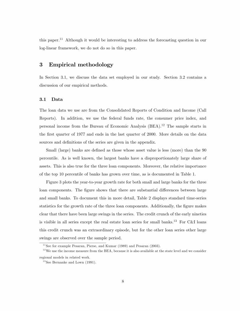
this paper.11 Although it would be interesting to address the forecasting question in our

log-linear framework, we do not do so in this paper.

3 Empirical methodology

In Section 3.1, we discuss the data set employed in our study. Section 3.2 contains a

discussion of our empirical methods.

3.1 Data

The loan data we use are from the Consolidated Reports of Condition and Income (Call

Reports). In addition, we use the federal funds rate, the consumer price index, and

personal income from the Bureau of Economic Analysis (BEA).12 The sample starts in

the �rst quarter of 1977 and ends in the last quarter of 2000. More details on the data

sources and de�nitions of the series are given in the appendix.

Small (large) banks are de�ned as those whose asset value is less (more) than the 90

percentile. As is well known, the largest banks have a disproportionately large share of

assets. This is also true for the three loan components. Moreover, the relative importance

of the top 10 percentile of banks has grown over time, as is documented in Table 1.

Figure 3 plots the year-to-year growth rate for both small and large banks for the three

loan components. The �gure shows that there are substantial di¤erences between large

and small banks. To document this in more detail, Table 2 displays standard time-series

statistics for the growth rate of the three loan components. Additionally, the �gure makes

clear that there have been large swings in the series. The credit crunch of the early nineties

is visible in all series except the real estate loan series for small banks.13 For C&I loans

this credit crunch was an extraordinary episode, but for the other loan series other large

swings are observed over the sample period.

11See for example Pesaran, Pierse, and Kumar (1989) and Pesaran (2003).12We use the income measure from the BEA, because it is also available at the state level and we consider

regional models in related work.13See Bernanke and Lown (1991).

8

Figure 4 plots, for large and small banks, the relative importance of the three loan

components in banks�loan portfolio. The graph shows that since the early eighties both

small and large banks have increased the share of real estate lending in their portfolio.

Small and large banks have o¤set the increased share of real estate lending in di¤erent

ways. Large banks have decreased the share of C&I loans, while small banks have decreased

the share of consumer loans in their portfolio.

3.2 Identi�cation

In Sections 3.2.1 and 3.2.2, we show how we estimate the behavior of the variables during

a monetary downturn and a non-monetary downturn of the same magnitude, respectively.

3.2.1 Monetary downturn

The standard procedure to study the impact of monetary policy on economic variables

is to estimate a structural VAR using a limited set of variables. Consider the following

VAR:14,15

Zt = B1Zt�1 + � � �+BqZt�q + ut; (4)

where Z 0t = [X01t; rt; X

02t], X1t is a (k1 � 1) vector with elements whose contemporaneous

values are in the information set of the central bank, rt is the federal funds rate, X2t is a

(k2 � 1) vector with elements whose contemporaneous values are not in the information

set of the central bank, and ut is a (k � 1) vector of residual terms with k = k1 + 1 + k2.

We assume that all lagged values are in the information set of the central bank. In order

to proceed one has to assume that there is a relationship between the reduced-form error

terms, ut, and the fundamental or structural shocks to the economy, "t. We assume that

14To simplify the discussion we do not display constants, trend terms, or seasonal dummies that are also

included.15 If there are cointegration restrictions, then the estimates of a VECM would be more e¢ cient. We

follow the literature and estimate a VAR. Using a VAR when a VECM is appropriate means that there is

some e¢ ciency loss but because of the rate T convergence, this e¢ ciency loss is small. On the other hand,

erroneously imposing cointegration would lead to a misspeci�ed system.

9

this relationship is given by:

ut = A"t; (5)

where A is a (k � k) matrix of coe¢ cients and "t is a (k � 1) vector of fundamental

uncorrelated shocks, each with a unit standard deviation. Thus,

E�utu

0t

�= A A

0: (6)

When we replace E[utu0t] by its sample analogue, we obtain k(k + 1)=2 conditions on

the coe¢ cients in A. Since A has k2 elements, k(k�1)=2 additional restrictions are needed

to estimate all elements of A. A standard practice is to obtain the additional k(k � 1)=2

restrictions by assuming that A is a lower-triangular matrix. Christiano, Eichenbaum, and

Evans (1999), however, show that to determine the e¤ects of a monetary policy shock one

can work with the less-restrictive assumption that A has the following block -triangular

structure:

A =

26664A11 0k1�1 0k1�k2

A21 A22 01�k2

A31 A32 A33

37775 (7)

where A11 is a (k1� k1) matrix, A21 is a (1� k1) matrix, A31 is a (k2� k1) matrix, A22 is

a (1� 1) matrix, A32 is a (k2 � 1) matrix, A33 is a (k2 � k2) matrix, and 0i�j is a (i� j)

matrix with zero elements. Note that this structure is consistent with the assumption

made above about the information set of the central bank.

We follow Bernanke and Blinder (1992) and many others by assuming that the federal

funds rate is the relevant policy instrument and that innovations in the federal funds rate

represent innovations in monetary policy. Moreover, throughout this paper we assume

that X1t is empty and that all other elements are, therefore, in X2t. Intuitively, X1t

being empty means that the Board of Governors of the Federal Reserve (FED) does not

respond to contemporaneous innovations in any of the variables of the system. While we

do believe that the FED can respond quite quickly to new information one has to keep in

mind that the data used here are revised data, which means that the value of a period t

10

observation in our data set was not available to the FED in period t. Rudebusch (1998)

points out that if the econometrician assumes that the FED responds to innovations in

the contemporaneous values of the available original data, but estimates the VAR with

revised data, the estimated coe¢ cients will be subject to bias and inconsistency.

3.2.2 Non-monetary downturn

Den Haan, Sumner, and Yamashiro (2007) compare the behavior of the variables during a

monetary downturn, that is, the responses to a negative monetary policy shock with the

behavior of the variables during a non-monetary downturn, that is, the responses during

a downturn of equal magnitude caused by real activity shocks. To be more precise, a non-

monetary downturn is caused by a sequence of output shocks such that output follows the

exact same path as it does during a monetary downturn.

The motivation for looking at these impulse response functions is the following. The

impulse response functions for the monetary downturn not only re�ects the direct responses

of the variables to an increase in the interest rate, but also the indirect responses to changes

in the other variables and, in particular, to the decline in real activity. This makes it

di¢ cult to understand what is happening, especially since a decline in real activity could

either increase or decrease the demand for bank loans.16 For example, if one observes

an increase in a loan component during a monetary downturn it could still be the case

that there is a credit crunch if a decline in real activity strongly increases the demand for

that particular loan component. That is, without the credit crunch this loan component

would have increased even more. By comparing the behavior of loan components during a

monetary downturn with a non-monetary downturn, of equal magnitude, one can get an

idea regarding the importance of the di¤erent e¤ects.

Den Haan, Sumner, and Yamashiro (2007) argue that the comparison of the behavior

of loans to monetary policy shocks and output shocks is useful in understanding what

happens during the monetary transmission mechanism. In this paper, the comparison is

16The reduction in real activity would reduce investment and, thus, the need for loans, but the reduction

in sales would increase inventories, which could increase the demand for loans.

11

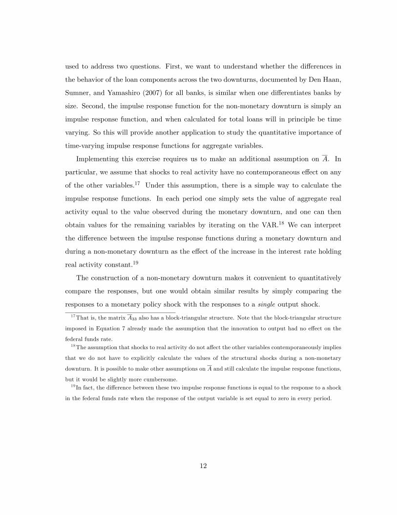
used to address two questions. First, we want to understand whether the di¤erences in

the behavior of the loan components across the two downturns, documented by Den Haan,

Sumner, and Yamashiro (2007) for all banks, is similar when one di¤erentiates banks by

size. Second, the impulse response function for the non-monetary downturn is simply an

impulse response function, and when calculated for total loans will in principle be time

varying. So this will provide another application to study the quantitative importance of

time-varying impulse response functions for aggregate variables.

Implementing this exercise requires us to make an additional assumption on A. In

particular, we assume that shocks to real activity have no contemporaneous e¤ect on any

of the other variables.17 Under this assumption, there is a simple way to calculate the

impulse response functions. In each period one simply sets the value of aggregate real

activity equal to the value observed during the monetary downturn, and one can then

obtain values for the remaining variables by iterating on the VAR.18 We can interpret

the di¤erence between the impulse response functions during a monetary downturn and

during a non-monetary downturn as the e¤ect of the increase in the interest rate holding

real activity constant.19

The construction of a non-monetary downturn makes it convenient to quantitatively

compare the responses, but one would obtain similar results by simply comparing the

responses to a monetary policy shock with the responses to a single output shock.

17That is, the matrix A33 also has a block-triangular structure. Note that the block-triangular structure

imposed in Equation 7 already made the assumption that the innovation to output had no e¤ect on the

federal funds rate.18The assumption that shocks to real activity do not a¤ect the other variables contemporaneously implies

that we do not have to explicitly calculate the values of the structural shocks during a non-monetary

downturn. It is possible to make other assumptions on A and still calculate the impulse response functions,

but it would be slightly more cumbersome.19 In fact, the di¤erence between these two impulse response functions is equal to the response to a shock

in the federal funds rate when the response of the output variable is set equal to zero in every period.

12

4 Responses of loan components

The results discussed in this section are based on a VAR that includes the three loan

components in addition to the federal funds rate, a price index, and a real activity measure.

Our benchmark speci�cation for the VAR includes one year of lagged variables, a constant,

and a linear trend. We also include quarterly dummies since the data from the Call reports

are not adjusted for seasonality.20

Output, the price level, and the interest rate response. Figure 5 plots the re-

sponses for output, the price level, and the federal funds rate. The results are consistent

with those in the literature. The federal funds rate gradually moves back to its pre-shock

value, with half of this adjustment occurring in the �rst year or so. Output declines, but

with a delay and only reaches its maximum decline after two years. When we feed the

VAR a series of output shocks that result in the same output decline, i.e., a non-monetary

downturn, then the interest rate declines, which is consistent with the monetary authority

following a Taylor rule. Finally, our results are subject to the price puzzle, with the price

level increasing after a monetary tightening.21

20 In addition, we estimated VARs for which the speci�cation was chosen using the Bayes Information

Criterion (BIC). We search for the best model among a set of models that allows, as regressors, the

variables mentioned above and a quadratic deterministic trend. BIC chooses a speci�cation that is more

concise then our benchmark speci�cation. The results are similar to those that are based on our benchmark

speci�cation.21Several papers have suggested alternative speci�cations of the VAR to avoid the price puzzle. Examples

are Christiano, Eichenbaum, and Evans (1999), Giordani (2004), and Romer and Romer (2004). Barth and

Ramey (2001) argue instead that there could be a cost channel that pushes prices up during a monetary

tightening and provide empirical evidence based on industry-level data to support their view. In our

experience, a positive price response is a very robust empirical �nding and we �nd little value in searching

for that VAR speci�cation that will give the desired price response. For example, Christiano, Eichenbaum,

and Evans (1999) �nd that adding an index for sensitive commodity prices solves the price puzzle in their

sample, but we �nd that this does not resolve the puzzle for our more recent samples. We also tried the

measure of monetary policy shocks proposed by Romer and Romer (2004) and reestimated the VAR over

the period for which this measure is available (1977 - 1996). We �nd that the price level sharply increases

during the �rst two quarters and after roughly one year has returned to its original level after which it

13

Average bank responses. Figure 6 reports the behavior of the three loan components

during a monetary and a non-monetary downturn using the series for all banks. The graph

shows that there are important di¤erences between the behavior of the three loan series

after a monetary tightening. Both real estate loans and consumer loans display sharp

negative decreases, although there is some delay before both begin to fall. In contrast,

C&I loans immediately increase and are signi�cantly positive for several years. Den Haan,

Sumner, and Yamashiro (2007) provide arguments related to hedging and banks safe-

guarding their capital adequacy ratio that can explain these movements. Here we take the

responses as given and analyze what they imply for the response of total loans.

The responses of the loan components during a non-monetary downturn gives a very

di¤erent picture. First, real estate loans decrease, but it is not a statistically signi�cant

decrease and the decrease is less than the one observed during a monetary during a mon-

etary downturn. Consumer loans are little changed in response to output shocks. Thus,

the behavior of real estate and consumer loans is consistent with the view that a monetary

tightening reduces the supply of bank loans by more than is predicted by the decline in

real activity. In contrast, C&I loans decrease during a non-monetary downturn.

Responses for small and large banks. In Figures 7 and 8 we plot the responses of

the three loan components for large banks (top 10 percentile) and small banks (bottom

90 percentile).22 In Section 3.1, we showed that there were substantial di¤erences in the

time-series behavior of the loan series for small and large banks and that the relative

importance of large banks had grown over time. Given these di¤erences it is remarkable

that the behavior of the loan components during both a monetary and a non-monetary

hovers around zero. Although not a solution to the price puzzle it is an improvement, since the price

level displays a persistent increase to a monetary tightening when innovations in the federal funds rate are

used as the monetary policy shock. More importantly, our other results are robust when alternative VAR

speci�cations are used to obtain di¤erent price responses.22When we replace the loan components with those of small or large banks, we �nd that the responses

for output, the federal funds rate, and the price level are similar to those in Figure 5 and are not reported.

14

downturn are so similar for the two types of banks.23 In particular, for both large and small

banks we observe that the responses for real estate and consumer loans decrease during a

monetary downturn, and not (or less) during a non-monetary downturn. Similarly, C&I

loans increase during a monetary downturn and decrease during a non-monetary downturn.

There are some intriguing quantitative di¤erences, however. For example, the response of

real estate loans is larger for small banks than it is for large banks. The opposite is true

for consumer loans.

5 Implied time-varying total loans responses

In Section 2, we showed that the impulse response function of a variable that is the sum

of variables in a VAR will, in general, be time varying. We can expect this to be more

of an issue when (i) the responses of the micro components di¤er and (ii) their relative

magnitudes change over time. In Section 3.1, we showed that the relative magnitudes of

loan components changed substantially over time both for large and for small banks and

in Section 4 we documented that C&I loans respond quite di¤erently to monetary policy

shocks than real estate and consumer loans.

To see how important the variation in initial conditions across the sample is, we calcu-

late the impulse response function for total loans for all observed initial values of the loan

components. The results are plotted in Figures 9, 10, and 11 for all banks, large banks,

and small banks, respectively. In each �gure, Panel A plots the response of total loans to

a shock in the federal funds rate and Panel B plots the di¤erence between the response of

total loans during a monetary downturn and a non-monetary downturn. The �gures show

that there is indeed substantial variation in the response of total loans, especially for large

banks and especially for the series that measures the di¤erence between the monetary and

the non-monetary downturn.

The top panel of Figure 9 shows that the total loan responses for all banks are, at �rst,

23Kashyap and Stein (1995) �nd more substantial di¤erences between the responses for large and small

banks in their speci�cations that do not control for changes in real activity. When they do control for

changes in real activity the di¤erences are strongly reduced.

15

always positive, then always turn negative, but the negative responses last at most three

years and for some initial conditions not even one year. The results in the bottom panel

correct the loan responses for the reduction in economic activity and show that there are

now numerous initial conditions for which the plotted loan response is always positive,

although there are also initial conditions for which the responses are negative for several

periods.

The results for large banks are very similar to those of all banks, although for large

banks there are some initial conditions for which the plotted loan responses are always

positive.

For small banks the responses are (at least in the �rst three years) consistently negative

and below those found for large banks.24 This is true both when the responses are and

when they are not corrected for the reduction in economic activity. Nevertheless, even for

small banks we �nd important quantitative di¤erences. In particular, for the 8th period

response the largest decrease of 0.476% is more than twice as large as the smallest decrease

of 0.238%.

Whereas the responses of the loan components displayed robust and signi�cant re-

sponses to a monetary tightening (but not in the same direction), the responses of total

loans� with the exception of the response for small banks� hover around zero in the �rst

couple of years. So, to some extent, the responses of total loans give a very incomplete

picture of what happens to bank lending during a monetary tightening.

We also compared the responses of total loans discussed above, which are based on a

VAR with loan components, with the response of total loans that are based on a VAR that

does not disaggregate total loans into its components. Of course, the response of total

loans from the latter would not be time varying. We �nd that for small banks the response

of total loans is similar to the average of the time-varying responses. For the large bank

and all banks series, however, the response is a bit above the time-varying responses.25

24This is consistent with the results of Kashyap and Stein (1995) and Kishan and Opiela (2000).25Given that the impulse responses of the loan components are actually estimated fairly precisely, the

reason is likely to be that the simple VAR, without loan components, has a hard time capturing the

dynamics of the system with only a relatively small number of lags.

16

The �gures discussed above do not make clear which impulse response function cor-

responds to what set of initial conditions. In Figure 12 we make this clear by plotting

the response eight quarters after the shock using as initial conditions the observed values

of the loan components in the period indicated on the x -axis. The patterns are similar

for both small and large banks. But as mentioned above, the response for small banks is

below the response for large banks. We can expect the response of an aggregate variable to

decrease over time if the variable with the response that is less negative becomes smaller

over time. That is true in our case since the fraction of C&I loans has decreased over time

and the response of C&I loans is, not only, less negative, it is positive. We see that the

responses for total loans indeed decrease over time although the results are not monotone.

The eight-quarter responses for total loans increase in the beginning of the sample and

reaches its maximum in the early eighties before a steady decline sets in. For small banks

the smallest value is observed in the early nineties after which the results stabilize. For

large banks a minor increase is observed during the nineties. To analyze the statistical

signi�cance of the amount of time variation we checked whether the di¤erence between the

response observed in the �rst quarter of 1983 (when the most positive value for large banks

is observed) and the response in the last quarter of the sample is signi�cantly di¤erent

from zero. For all three loans series we �nd that the di¤erence is signi�cant at the 5%

level.26

6 Time-varying total loans responses

Figure 12 predicts a particular pattern for the response of total bank loans to a monetary

tightening. There are basically two u-shaped patterns with the responses reaching a max-

imum around 1983, which is exactly when the share of C&I loans, that have a positive

response, reaches its highest value. The question arises whether one would �nd something

similar if one would try to directly estimate the response of total loans using a method-

ology that allows the response to be time varying. The problem is that there are several

26 In each Monte Carlo replication of our bootstrap procedure we calculated this di¤erence and we checked

whether the 5% percentile was positive.

17

ways to do this, for example, Bayesian VARs with time-varying coe¢ cients or standard

VARs using rolling samples. The problem is enhanced by the fact that numerous choices

have to be made in implementing these techniques. The implied responses for total loans

documented in Figures 9 through 12 are based on a snapshot, i.e., what the total loans

responses are for the initial conditions observed in one particular period. Consequently,

with direct estimation the sample period should be quite small, but this would make it

di¢ cult to precisely estimate the many parameters in the VAR.

Despite all these caveats, it would be interesting to see whether there is at least some

correspondence between the implied time-varying total loan responses and those found by

direct estimation. To investigate whether the directly estimated total loans response is

time varying, we use relatively short rolling samples. Using short samples means that we

have to make several changes to safeguard the degrees of freedom. Most importantly, we

focus on the monthly H.8 loan data. These data are of lesser quality than the Call Report

data, but are available on a monthly frequency increasing the degrees of freedom.27

Another aspect to keep in mind is that the responses of the loan components are, of

course, also changing, especially if they are estimated with short rolling windows. To see

whether the changes in the relative magnitudes of the loan components play a role in

explaining the changes in the directly estimated total loan responses, we do the following.

In each sample, we estimate the 10th-quarter (i.e., 30th-month) total loan response.

Next, we estimate the 10th-quarter loan component responses and construct an indirect

estimate of the 10th-quarter total loan response by taking the weighted sum of the loan

component responses. The weights used are �xed averages, equal to the observed averages

over the whole sample.

In the �gures, we plot the di¤erence between the directly estimated and the constructed

total loan response. The constructed total loan response does not take into account the

source of time variation emphasized in this paper, namely changing relative magnitudes

of the components. So the question is whether the plotted di¤erence can be explained by

27See Den Haan, Sumner, and Yamashiro (2002) for a comparison of H8 and Call Report data. We also

exclude the price index from the VAR to increase the degrees of freedom. We did not �nd this to a¤ect

the results.

18

the changing weights. To answer this question, we plot in the �gures also the 10th-quarter

response constructed using time-varying weights and �xed loan component responses.28

For the �xed loan component impulse response function, we use the average across the

rolling windows.

Figure 13 reports the results for the total loans responses during a monetary tightening

and �gure 14 reports the results for the di¤erence between the responses during a monetary

and a non-monetary downturn. The top panel in each graph shows the results for rolling

windows of 25 years and the bottom panel shows the results for rolling windows of 30

years.

In all four cases, there is a general tendency for the changes in the total loan response

predicted using only changes in the weights (the dotted line) to move together with the

changes in the total loan response that are not explained by changes in the responses of

the components themselves (the solid line). More than a general comovement was not to

be expected. The weights change relatively slowly. Consequently, the changes in the total

loan response due to changes in the weights occur gradually. In contrast, the counterpart is

obtained using rolling windows and is, thus, subject to quite a bit of sampling variation.29

7 Concluding Comments

The time-varying responses for total bank loans reported in this paper are from a VAR with

constant coe¢ cients. The question arises as to whether the coe¢ cients of the VAR remain

the same when the relative magnitudes of the loan components display such substantial

changes.30 It is even a possibility that banks behave in such a way to keep the response

of total loans to monetary policy shocks constant when the relative magnitude of the loan

28Also, the mean is taken out to make the di¤erence between the two total loans responses comparable

to the predicted level response.29For this reason, one should not take this exercise too seriously. The results only look nice for a certain

sample length. If the length of the rolling windows becomes too short, then the estimates are very volatile.

If the lengths become too long, then there is no variation left to explain. We have no argument for choosing

the adopted window lengths other than that these generate the desired general comovement.30The VAR does include a deterministic trend term, but this only captures changes in the constant term.

19

components change. In this case, it might be better to actually use a VAR that only

includes total loans.

Obviously one always has to be aware of the possibility that behavior changes over time.

The main point of this paper is that impulse response functions of aggregated variables can

change over time even if the behavior of the micro components does not change over time.

In this paper we have demonstrated that this is a quantitatively important phenomenon

for total loans.

A Data sources

The Call Report bank balance-sheet data are available online.31 Also, a description on

how they are constructed can be found in Den Haan, Sumner, and Yamashiro (2002). In

this paper we use the "level series".

Quarterly observations for the CPI and federal funds rate are constructed by taking

an average of the monthly observations downloaded from http://research.stlouisfed.org

(CPI) and http://www.federalreserve.gov (federal funds rate). The quarterly income vari-

able used is earnings (by place of work) from the Bureau of Economic Analysis. It was

downloaded from http://www.bea.doc.gov/. In related work we examine the e¤ect of re-

gional responses to monetary policy shocks and the advantage of this real activity measure

is that it is available at the regional level. The results are very similar, however, if we use

GDP and its de�ator.

The monthly data used in Section 6 are the H.8 bank loan data. These are downloaded

from http://www.federalreserve.gov. The industrial production data are downloaded from

http://research.stlouisfed.org.

References

Barth, M. J. I., and V. A. Ramey (2001): �The Cost Channel of Monetary Transmis-

sion,�NBER Macroeconomics Annual, 16, 199�256.

31At http://www1.feb.uva.nl/mint/wdenhaan/data.htm

20

Bernanke, B. S., and A. S. Blinder (1992): �The Federal Funds Rate and the Chan-

nels of Monetary Transmission,�American Economic Review, 82, 901�921.

Bernanke, B. S., and C. S. Lown (1991): �The Credit Crunch,�Brookings Papers on

Economic Activity, 2, 204�239.

Christiano, L. J., M. Eichenbaum, and C. L. Evans (1999): �Monetary Policy

Shocks: What Have We Learned and to What End?,�in Handbook of Macroeconomics,

ed. by J. B. Taylor, and M. Woodford, pp. 65�148. North-Holland, Amsterdam.

Den Haan, W. J., S. W. Sumner, and G. Yamashiro (2002): �Construction of

Aggregate and Regional Bank Data Using the Call Reports: Data Manual,�Unpublished

manuscript, University of Amsterdam.

(2007): �Bank Loan Portfolios and the Monetary Transmission Mechanism,�

Journal of Monetary Economics, 54, 904�924.

(2009): �Bank Loan Portfolios and the Canadian Monetary Transmission Mech-

anism,�Canadian Journal of Economics, 42, 1150�1175.

Gertler, M., and S. Gilchrist (1993): �The Cyclical Behavior of Short-Term Busi-

ness Lending: Implications for Financial Propagation Mechanisms,�European Economic

Review, 37, 623�631.

Giordani, P. (2004): �An Alternative Explanation of the Price Puzzle,� Journal of

Monetary Economics, 51, 1271�1296.

Granger, C. W. (1980): �Long Memory Relationships and the Aggregation of Dynamic

Models,�Journal of Econometrics, 14, 227�238.

Kashyap, A. K., and J. C. Stein (1995): �The Impact of Montetary Policy on Bank

Balance Sheets,�Carnegie-Rochester Series on Public Policy, 42, 151�195.

Kishan, R., and T. Opiela (2000): �Bank Size, Bank Capital, and the Bank Lending

Channel,�Journal of Money, Credit and Banking, 32, 121�141.

21

Pesaran, M. H. (2003): �Aggregation of Linear Dynamic Models: An Application to

Life-Cycle Consumption Models under Habit Formation,�Economic Modelling, 20, 383�

415.

Pesaran, M. H., R. G. Pierse, and M. S. Kumar (1989): �Econometric Analysis of

Aggregation in the Context of Linear Prediction Models,�Econometrica, 57, 861�888.

Potter, S. (1999): �Nonlinear Time Series Modelling: An Introduction,� Journal of

Economic Surveys, 13, 505�528.

Romer, C. D., and D. H. Romer (2004): �A New Measure of Monetary Shocks: Deriva-

tion and Implications,�American Economics Review, 94, 1055�1084.

Rudebusch, G. D. (1998): �Do Measures of Monetary Policy in a VAR Make Sense?,�

International Economic Review, 39, 907�931.

van Garderen, K. J., K. Lee, and M. H. Pesaran (2000): �Cross-Sectional Aggre-

gation of Non-Linear Models,�Journal of Econometrics, 95, 285�331.

22

Table 1: Increased importance of large banks

1977Q1 2000Q4large banks small banks large banks small banks

C&I 83% 17% 91% 9%real estate 67% 33% 82% 18%consumer 65% 35% 89% 11%

23

Table 2: Summary statistics for growth rates

C&I real estate consumerlarge small large small large small

average 1.74% 1.06% 2.68% 1.87% 1.91% 0.32%standard deviation 2.44% 2.07% 1.57% 1.31% 2.88% 2.07%autocorrelation 0.20 0.52 0.55 0.63 0.26 0.44

24

Figure 1: Impulse response function of zt for different initial values of ln(z1,t/ z2,t)

0

0.05

0.1

0.15

0.2

0.25

0.3

0.35

0.4

0.45

0 5 10 15 20 25 30 35

time

-2 st. dev. -1 st. dev. average +1st. dev. +2 st. dev. Note: This graph plots the impulse response function of ln(zt) in response to a one-standard-deviation shock in e when the initial value of ln(z1,t/ z2,t) varies from being two standard deviations below to two standard deviations above its average value (of zero)

Figure 2: Impulse response function of zt for first and second shock

0

0.05

0.1

0.15

0.2

0.25

0.3

0.35

0.4

0.45

0.5

0 5 10 15 20 25 30 35

time

low initial value

effect of first and second shock for high initial value of variable micro component

first shock

second shock

Note: This graph plots the impulse response function of ln(zt) in response to a one-standard-deviation shock in e (solid line) and the impulse response function of ln(zt) in response to a subsequent shock of equal magnitude (dashed line) when the value of ln(z1,t/ z2,t) at the time of the first shock occurs is equal to two standard deviations below and two standard deviations above its average value.

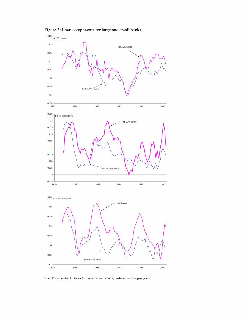
Figure 3: Loan components for large and small banks

-0.15

-0.1

-0.05

0

0.05

0.1

0.15

0.2

0.25

1975 1980 1985 1990 1995 2000

top 10% banks

bottom 90% banks

A: C&I loans

-0.025

0

0.025

0.05

0.075

0.1

0.125

0.15

0.175

0.2

0.225

1975 1980 1985 1990 1995 2000

top 10% banks

bottom 90% banks

B: Real estate loans

-0.1

-0.05

0

0.05

0.1

0.15

0.2

0.25

1975 1980 1985 1990 1995 2000

top 10% banks

bottom 90% banks

C: Consumer loans

Note: These graphs plot for each quarter the natural log growth rate over the past year.

Figure 4: Banks’ loan portfolio

0

0.1

0.2

0.3

0.4

0.5

0.6

0.7

1975 1980 1985 1990 1995 2000

C&I loansreal estate loans

consumer loans

A: Large banks

0

0.1

0.2

0.3

0.4

0.5

0.6

0.7

1975 1980 1985 1990 1995 2000

A: Small banks

real estate loans

C&I loans

consumer loans

Note: These graphs plot the share of the indicated loan component as a fraction of the sum of the three loan components.

Figure 5: Impulse responses for output, price level, and federal funds rate (VAR with “all bank” loan series)

-0.4%

-0.3%

-0.2%

-0.1%

0.0%

0.1%

0.2%

0.3%

0.4%

0 1 2 3 4 5 6 7

time (years)

□ : 10% significance level■ : 5% significance level

A: Output

-0.4

-0.2

0.0

0.2

0.4

0.6

0.8

1.0

0 1 2 3 4 5 6 7

time (years)

monetary downturn

non-monetary downturn

B: Federal funds rate □ : 10% significance level■ : 5% significance level

-0.20%

-0.15%

-0.10%

-0.05%

0.00%

0.05%

0.10%

0.15%

0.20%

0.25%

0.30%

0.35%

0 1 2 3 4 5 6 7

time (years)

monetary downturn


C: Price level □ : 10% significance level■ : 5% significance level

Note: These graphs plot the response of the indicated variable to a one-standard deviation federal funds rate shock, i.e., a monetary downturn. In Panels B and C the curve labelled “non-monetary downturn” plots the time path of the federal funds rate and consumer price index following a sequence of output shocks that generates a time path for output that is identical to that of the monetary downturn plotted in panel A. The results are based on the benchmark specification. Open squares indicate a significant response at the 10% level and a solid square indicates a significant response at the 5% level (both one-sided tests).

Figure 6: Loan impulse responses - All banks

-1.5%

-1.0%

-0.5%

0.0%

0.5%

1.0%

1.5%

0 1 2 3 4 5 6 7

time (years)

monetary downturn



A: Commercial and industrial loans

-0.8%

-0.6%

-0.4%

-0.2%

0.0%

0.2%

0.4%

0.6%

0.8%

0 1 2 3 4 5 6 7

time (years)


monetary downturn



-1.4%

-1.2%

-1.0%

-0.8%

-0.6%

-0.4%

-0.2%

0.0%

0.2%

0.4%

0.6%

0 1 2 3 4 5 6 7

time (years)


monetary downturn


C: Consumer loans

Note: These graphs plot the response of the indicated loan variable to a one-standard deviation federal funds rate shock, i.e., a monetary downturn. The curves labelled “non-monetary downturn” plot the time path of the loan variable following a sequence of output shocks that generates a time path for output that is identical to that of the monetary downturn (plotted in panel A of Figure 4.1). The results are based on the benchmark specification. Open squares indicate a significant response at the 10% level and a solid square indicates a significant response at the 5% level (both one-sided tests).

Figure 7: Loan impulse responses - Large banks

-1.5%

-1.0%

-0.5%

0.0%

0.5%

1.0%

1.5%

0 1 2 3 4 5 6 7

time (years)

monetary downturn

non-monetary downturn □ : 10% significance level■ : 5% significance level


-0.6%

-0.4%

-0.2%

0.0%

0.2%

0.4%

0.6%

0.8%

0 1 2 3 4 5 6 7

time (years)


monetary downturn □ : 10% significance level■ : 5% significance level


-2.0%

-1.5%

-1.0%

-0.5%

0.0%

0.5%

1.0%

0 1 2 3 4 5 6 7

time (years)



C: Consumer loans

Note: These graphs plot the response of the indicated loan variable to a one-standard deviation federal funds rate shock, i.e., a monetary downturn. The curves labelled “non-monetary downturn” plot the time path of the loan variable following a sequence of output shocks that generates a time path for output that is identical to that of the monetary downturn. The results are based on the benchmark specification. Open squares indicate a significant response at the 10% level and a solid square indicates a significant response at the 5% level (both one-sided tests).

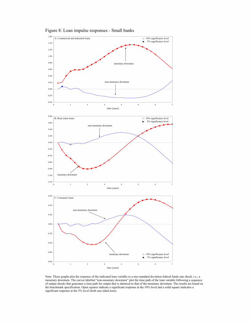
Figure 8: Loan impulse responses - Small banks

-0.4%

-0.2%

0.0%

0.2%

0.4%

0.6%

0.8%

1.0%

1.2%

1.4%

1.6%

0 1 2 3 4 5 6 7

time (years)

monetary downturn




-1.2%

-1.0%

-0.8%

-0.6%

-0.4%

-0.2%

0.0%

0.2%

0.4%

0.6%

0.8%

0 1 2 3 4 5 6 7

time (years)


monetary downturn



-0.8%

-0.6%

-0.4%

-0.2%

0.0%

0.2%

0.4%

0.6%

0 1 2 3 4 5 6 7

time (years)



C: Consumer loans

Note: These graphs plot the response of the indicated loan variable to a one-standard deviation federal funds rate shock, i.e., a monetary downturn. The curves labelled “non-monetary downturn” plot the time path of the loan variable following a sequence of output shocks that generates a time path for output that is identical to that of the monetary downturn. The results are based on the benchmark specification. Open squares indicate a significant response at the 10% level and a solid square indicates a significant response at the 5% level (both one-sided tests).

Figure 9: Implied total loans impulses for VAR with loan components - All banks

-0.50%

-0.30%

-0.10%

0.10%

0.30%

0.50%

0.70%

0 1 2 3 4 5 6 7

time (years)

A: Total loans impulse response function

-0.30%

-0.20%

-0.10%

0.00%

0.10%

0.20%

0.30%

0.40%

0.50%

0.60%

0.70%

0 1 2 3 4 5 6 7

time (years)

B: Difference with non-monetary downturn

Note: Panel A plots the impulse response function of total loans for all initial conditions observed in the sample. Panel B plots the difference between the response of total loans during a monetary downturn and a non-monetary downturn.

Figure 10: Implied total loans impulses for VAR with loan components - Large banks

-0.50%

-0.30%

-0.10%

0.10%

0.30%

0.50%

0.70%

0 1 2 3 4 5 6 7

time (years)


-0.30%

-0.20%

-0.10%

0.00%

0.10%

0.20%

0.30%

0.40%

0.50%

0.60%

0.70%

0.80%

0 1 2 3 4 5 6 7

time (years)



Figure 11: Implied total loans impulses for VAR with loan components - Small banks

-0.50%

-0.30%

-0.10%

0.10%

0.30%

0.50%

0.70%

0 1 2 3 4 5 6 7

time (years)


-0.60%

-0.40%

-0.20%

0.00%

0.20%

0.40%

0.60%

0.80%

1.00%

1.20%

0 1 2 3 4 5 6 7

time (years)



Figure 12: 8th-quarter implied total bank loans response for VAR

-0.60%

-0.50%

-0.40%

-0.30%

-0.20%

-0.10%

0.00%

0.10%

0.20%

0.30%

1976 1980 1984 1988 1992 1996 2000

large banks

small banks

all banks

Note: This graph plots the 8th-quarter impulse response of indicated total loans series using as initial values those observed in the period indicated on the x-axis.

Figure 13: Variation of total loan responses explained by changing weights – H.8 data (Responses to monetary policy shock)

-0.08%

-0.06%

-0.04%

-0.02%

0.00%

0.02%

0.04%

0.06%

0.08%

1976 1978 1980 1982 1984 1986 1988 1990 1992

A: Rolling 25-year windows

Predicted difference based on changing weights and unchanging loan component responses

Actual difference between i) changing total loans response & ii) weighted sum of changing loan component responses (fixed weights)

-0.08%

-0.06%

-0.04%

-0.02%

0.00%

0.02%

0.04%

1976 1978 1980 1982 1984 1986 1988

B: Rolling 30-year windows



Note: The solid lines represent the difference between the 10th-quarter impulse total loans response directly estimated and the indirectly calculated response using the weighted sum of the responses of the loan components using fixed weights. All responses are estimated using rolling windows with the value on the x-axis at the midpoint of the sample. The dotted line represents the weighted sum of the (fixed) average loan component responses and time-varying weights.

Figure 14: Variation of total loan responses explained by changing weights – H.8 data (Difference between responses during a monetary and non-monetary downturn)

-0.06%

-0.04%

-0.02%

0.00%

0.02%

0.04%

0.06%

0.08%

0.10%

1976 1978 1980 1982 1984 1986 1988 1990 1992

A: Rolling 25-year windows



-0.12%

-0.10%

-0.08%

-0.06%

-0.04%

-0.02%

0.00%

0.02%

0.04%

0.06%

0.08%

0.10%

1976 1978 1980 1982 1984 1986 1988

B: Rolling 30-year windows



Note: The solid lines represent the difference between the 10th-quarter impulse total loans response directly estimated and the indirectly calculated response using the weighted sum of the responses of the loan components using fixed weights. All responses are estimated using rolling windows with the value on the x-axis at the midpoint of the sample. The dotted line represents the weighted sum of the (fixed) average loan component responses and time-varying weights.

bank loan components and the time ... - wouter den haan loan components and the time-varying...

Documents