bank failure prediction: a two-step survival time approach · bank failure prediction: a two-step...

48 IFC Bulletin No 28

Bank failure prediction: a two-step survival time approach

Michael Halling1 and Evelyn Hayden2, 3

1. Introduction

The financial health of the banking industry is an important prerequisite for economic stability and growth. As a consequence, the assessment of banks’ financial condition is a fundamental goal for regulators. As on-site inspections are usually very costly, take a considerable amount of time and cannot be performed with high frequency, in order to avoid too frequent inspections without loosing too much information, supervisors also monitor banks’ financial condition off-site. Typically, off-site supervision is based on different information available to supervisors, which includes mainly balance sheet and income statement data, data on the residual maturity of obligations, and credit register data about loans granted to individual borrowers above a given threshold.

Off-site analysis uses different methods, such as CAMEL-based approaches, statistical techniques and credit risk models. Early warning systems based on statistical techniques reflect the rapidity with which the performance of a bank responds to a changing macroeconomic cycle, the conditions on the monetary and financial markets, and the interventions of the supervisory authority. Therefore, for the time being, statistical techniques like discriminant analysis and probit/logit regressions play a dominant role in off-site banking supervision. They allow an estimate to be made of the probability that a bank with a given set of characteristics will fall into one of two or more states, most often failure/non-failure, reflecting the bank’s financial condition over an interval of time implied by the study design, usually defined as one year.

An interesting academic discussion addresses the different advantages and disadvantages of statistical default prediction models as opposed to structural credit risk models. While statistical approaches do not explicitly model the underlying economic relationships, structural models emerge from corporate finance theory. However, there is ample empirical evidence that structural models perform poorly in predicting corporate bond spreads and corporate bankruptcy. Another problem in applying structural models to bank regulation is usually the lack of market data. For example, in the last decade in Austria only about 1% of a total of 1100 existing banks were listed on a stock exchange. Therefore, we focus on statistical bank default prediction in this paper.

There is a quite extensive literature concerning the use of discriminant analysis and logit/probit regressions that distinguish between “good” and “bad” banks. Other statistical

1 Michael Halling, Department of Finance, University of Vienna, Brünnerstraße 72, A-1210 Vienna.

Tel: +43 1 4277 38081. E-Mail: [email protected]. 2 Banking Analysis and Inspections Division, Österreichische Nationalbank (Austrian National Bank),

Otto-Wagner-Platz 3, POB 61, A-1011 Vienna. Tel: +43 1 40420 3224. E-Mail: [email protected]. 3 This article contains the authors’ personal opinions and does not necessarily reflect the point of view of the

Austrian National Bank.

We thank participants of the Austrian Working Group on Banking and Finance Meeting 2004 and of the C.R.E.D.I.T. 2005 Conference for their valuable comments. Furthermore, we are grateful to Pierre Mella-Barral for discussions on the issue of default prediction.

IFC Bulletin No 28 49

models that have not received appropriate attention so far are based on survival time analysis. Here the time to default is estimated explicitly in addition to default probabilities. This is an important piece of information in banking supervision, as regulators require information about troubled banks with sufficient lead time to take preventive or remedial actions at problem banks. Bank regulators may prefer to examine the entire survival profile (ie the change in the estimated probability of survival/default over time) for each bank and assess the probability of failure at any point in time in terms of the cost of on-site examinations versus the cost of misclassifications.

The two-step survival time procedure presented in this paper combines a multi-period logit model and a survival time model. In the first step, we determine whether a bank is at risk to default using the output of a basic logit model. We define different criteria to distinguish between “good” and “bad” banks. For banks that become at-risk during our sample period according to the first step of our procedure, we estimate a survival time model in the second step to predict default and estimate the time to default as accurately as possible. The rationale for this approach is based on our belief that the covariates that determine whether a bank is in good or bad shape differ from the variables that explain how long at-risk banks survive.

By following this approach, we extend the existing literature in three ways. First, we propose a statistical method to determine the point in time at which a bank becomes at-risk and, consequently, derive an estimate for a meaningful time to default definition that captures the status of the bank. In contrast, existing papers either assume that all banks automatically become at-risk when the observed sample starts or that banks become at-risk when they are founded. In the first case, the time to default is not bank-specific, does not take into account banks’ financial condition, and actually equals calendar time dummies. In the latter case, the measure is bank-specific but independent of the bank’s current economic situation. Second, we distinguish between “healthy” and “ill” (at-risk) banks as we expect that different economic relationships may exist between independent and dependent variables in each sub-sample. Third, we use sophisticated survival time models that more closely fit the characteristics of bank failure prediction. The standard model in the literature is the Cox proportional hazards model, which assumes that the observed covariates are constant. However, typical explanatory variables, like banks’ balance sheets or macroeconomic data, change with time. Furthermore, banks’ financial conditions are not observed continuously but rather at discrete points in time. Appropriate statistical techniques exist to deal with this.

We empirically evaluate our proposed two-step approach by using Austrian bank data. We compare our two-step models with the logit model currently in use at the Austrian National Bank and to a survival time model that assumes that all banks become at-risk when they are founded. Both benchmark models are estimated for the entire sample of banks and, consequently, are one-step approaches. Except for the logit model of the Austrian National Bank, all other models are derived by evaluating the predictive power of 50 explanatory variables – the final contribution of our paper.

We find that the two-step survival time models outperform both one-step models with respect to out-of-sample performance. However, survival time itself is not the main driver of the performance improvement. This results, rather, from the estimation of an individual predictive model for at-risk banks. We find that the models for at-risk banks contain some of the same variables as the benchmark logit model (e.g. ratios capturing credit risk) and some different variables (e.g. bank size relative to its geographically closest peers, management quality and the policy to donate and dissolve loss provisions). This supports the argument that, in comparison to the entire bank population, different variables are required to predict failure for at-risk banks accurately.

The paper is organized as follows: in the next section, we introduce the two-step approach, explain the criteria to determine whether a bank is at risk, and briefly review the statistical


foundations. Section 3 describes the empirical study, the data used, and the way we build the survival time models. Section 4 presents the empirical results, and section 5 concludes.

2. Two-step survival time model

Our goal is to develop a two-step survival time approach to predict bank failure because (a) time to default might be an important type of information for regulators, and (b) predictive relationships might differ between at-risk banks and the entire sample of banks. Given these goals, there are two main challenges: (a) to identify a good measure for the time to default, and (b) to estimate a survival time model that accounts for important characteristics of bankruptcy data.

2.1 Identification of “at-risk” banks (first step) In order to measure the time to default appropriately and to select the banks that are at risk, we propose using a standard multi-period logit model4 to determine which banks become at-risk at which point in time. In other words, we use the multi-period logit model’s output to assess the health status of banks. The logit model that we use for this purpose is the current major off-site analysis model applied at the Austrian National Bank (see Hayden and Bauer (2004)). This multi-period logit model comprises 12 explanatory variables, including one capturing bank characteristics, four assessing credit risk exposure, two considering capital structure, four measuring profitability and one accounting for the macroeconomic environment (see section 4.1 for more details).

We define the following three criteria based on this model’s quarterly output in order to determine whether a bank becomes at-risk at a specific point in time:

• At-risk definition 1 (2xLevel): a bank is at risk if the output exceeds the (statistically optimized) threshold of 1.6% in two subsequent three-month periods.

• At-risk definition 2 (Growth): a bank becomes at-risk if the model’s output has grown by more than (statistically optimized) 1.1% in the previous period.

• At-risk definition 3 (Combined): a bank becomes at-risk if definition 1 and/or definition 2 are fulfilled.

At-risk definition 1 (2xLevel) extends over two periods because the logit model output shows some volatility and therefore a criterion based on only one observation would too quickly assign at-risk status to a bank. While definition 1 focuses on the level of the logit model’s output, definition 2 (Growth) takes a more dynamic perspective and looks at the change of the model’s output between two subsequent periods of time. The argument for this definition is that even for good banks (ie banks with a low model output), a relatively large increase in the model output from one period to the next could indicate that the bank’s status has deteriorated and that the bank is at risk.

So far, papers have usually assumed that all banks become at-risk either when they are founded (e.g. Shumway (2001), although he is not estimating a survival time model in our opinion) or when the observed sample starts (e.g. Lane et al. (1986)). We do not think that these two approaches are especially meaningful, for two reasons. First, the time information

4 Note that what we call a multi-period logit model is called a hazard model in Shumway (2001). Terminology in

the literature is not at all homogeneous, as terms like logit models, survival time models and hazard models are frequently used interchangeably.


derived from these models does not capture what we want to capture. If time to default is measured relative to the same point in time (ie the starting period of the sample) for all banks, then the time to default is reduced to calendar year dummies and does not contain any bank-specific information. If, on the other hand, bank age is used as a proxy for time to default, it remains to be shown that this is a good proxy as it ignores any developments since the bank’s foundation. Intuitively we question this hypothesis and empirically investigate it in this paper. Second, both approaches consider all banks to be at risk. In our opinion, this does not really fit with one fundamental idea of survival time analysis, namely that different relationships between independent and dependent variables occur within the sample of all subjects and the sample of at-risk subjects. In a medical setting, for example, one would not expect that the best predictors for a person’s life expectancy would be identical to the factors that influence the survival time of people suffering from a major disease.

Our approach is also based on an important assumption, namely that no bank is at risk before our sample period starts. However, this assumption will (hopefully slightly) bias our time-to-default variables, while it should not have an influence on the sample of banks that are identified as at-risk. In any case, we believe that our assumption is far less problematic than the previously discussed assumptions. Another challenge of our approach is to determine the appropriate thresholds for defining at-risk banks. Both thresholds used in definitions 1 and 2 were statistically optimized in the sense that they represent the threshold levels with the best performance to correctly classify bank defaults when evaluating the power of different thresholds. Finally, note that once a bank is at risk, it cannot revert to “normal” status, but remains “at-risk”. Allowing banks to switch between being at risk and not at risk would represent a potentially interesting but not straightforward extension of our study.

2.2 Discrete survival time model with time-varying covariates While the Cox proportional hazards model represents the most popular survival time model, we decided to implement a discrete survival time model. We use this model because (a) we observe defaults only at discrete points in time and (b) we have a positive probability of ties. Both these characteristics of our environment conflict with important assumptions underlying the Cox proportional hazards model.

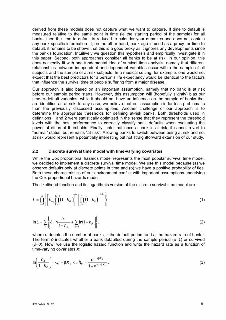
The likelihood function and its logarithmic version of the discrete survival time model are

( ) ( )∏ ∏∏=

δ−τ

=

δ−τ

=τ

⎪⎭

⎪⎬⎫

⎪⎩

⎪⎨⎧

⎥⎦

⎤⎢⎣

⎡−⎥

⎦

⎤⎢⎣

⎡−=

n

i jij

kiki

ii

ii

ihhhL

1

1

1

1

111 (1)

( )∑ ∑=

τ

=τ

τ

⎪⎭

⎪⎬⎫

⎪⎩

⎪⎨⎧

−+−

δ=n

i kik

i

ii

i

i

i hh

hL

1 11ln

1lnln , (2)

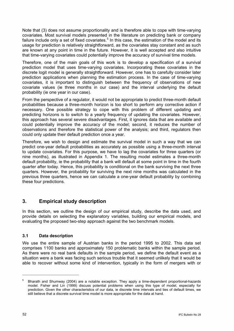
where n denotes the number of banks, τi the default period, and hi the hazard rate of bank i. The term δ indicates whether a bank defaulted during the sample period (δ=1) or survived (δ=0). Now, we use the logistic hazard function and write the hazard rate as a function of time-varying covariates X:

itt

itt

X

X

itittit

it

eehX

hh

β+α

β+α

+=⇔β+α=⎟⎟

⎠

⎞⎜⎜⎝

⎛− 11

ln . (3)


Note that (3) does not assume proportionality and is therefore able to cope with time-varying covariates. Most survival models presented in the literature on predicting bank or company failure include only a set of fixed covariates.5 In this case, the estimation of the model and its usage for prediction is relatively straightforward, as the covariates stay constant and as such are known at any point in time in the future. However, it is well accepted and also intuitive that time-varying covariates could potentially improve the accuracy of survival time models.

Therefore, one of the main goals of this work is to develop a specification of a survival prediction model that uses time-varying covariates. Incorporating these covariates in the discrete logit model is generally straightforward. However, one has to carefully consider later prediction applications when planning the estimation process. In the case of time-varying covariates, it is important to distinguish between the frequency of observations of new covariate values (ie three months in our case) and the interval underlying the default probability (ie one year in our case).

From the perspective of a regulator, it would not be appropriate to predict three-month default probabilities because a three-month horizon is too short to perform any corrective action if necessary. One possible strategy to cope with this problem of different updating and predicting horizons is to switch to a yearly frequency of updating the covariates. However, this approach has several severe disadvantages. First, it ignores data that are available and could potentially improve the accuracy of the model; second, it reduces the number of observations and therefore the statistical power of the analysis; and third, regulators then could only update their default prediction once a year.

Therefore, we wish to design and estimate the survival model in such a way that we can predict one-year default probabilities as accurately as possible using a three-month interval to update covariates. For this purpose, we have to lag the covariates for three quarters (or nine months), as illustrated in Appendix 1. The resulting model estimates a three-month default probability, ie the probability that a bank will default at some point in time in the fourth quarter after today. Hence, this probability is conditional on the bank surviving the next three quarters. However, the probability for surviving the next nine months was calculated in the previous three quarters, hence we can calculate a one-year default probability by combining these four predictions.

3. Empirical study description

In this section, we outline the design of our empirical study, describe the data used, and provide details on selecting the explanatory variables, building our empirical models, and evaluating the proposed two-step approach against the two benchmark models.

3.1 Data description We use the entire sample of Austrian banks in the period 1995 to 2002. This data set comprises 1100 banks and approximately 150 problematic banks within the sample period. As there were no real bank defaults in the sample period, we define the default event as a situation were a bank was facing such serious trouble that it seemed unlikely that it would be able to recover without some kind of intervention, typically in the form of mergers with or

5 Bharath and Shumway (2004) are a notable exception. They apply a time-dependent proportional-hazards

model. Fisher and Lin (1999) discuss potential problems when using this type of model, especially for prediction. Given the other characteristics of our data, ie discrete time intervals and ties of default times, we still believe that a discrete survival time model is more appropriate for the data at hand.


allowances from affiliated banks. In doing so, we follow the definition of problematic banks that was employed for the development of the logit model currently applied by the Austrian National Bank (see Hayden and Bauer (2004)).

As far as explanatory variables are concerned, different data sources have been used. Similar to the definition of problematic banks, we stick to the same data material that has been collected by the Austrian National Bank in order to develop its multi-period logit model. This data pool comprises partly monthly and yearly, but primarily quarterly, data items from banks’ balance sheets, profit and loss statements, and regulatory reports. Moreover, additional information on large loans and macroeconomic variables has been used. Based on these data sources, approximately 280 potential explanatory variables covering bank characteristics, market risk, credit risk, operational risk, liquidity risk, reputation risk, capital structure, profitability, management quality, and macroeconomic environment have been defined. The actual data frequency used in this paper is quarterly.

3.2 Model building With respect to model building and model evaluation, we follow a standard statistical procedure that has been applied similarly by the Austrian National Bank in order to develop its logit model. By doing so, we ensure that the derived models are indeed comparable. Hence, we separate the available data set into one in- and one out-of-sample subset by randomly splitting the data into two sub-samples. The first, which contains approximately 70% of all observations, is used to estimate the model, while the remaining data is left for an out-of-sample evaluation. When splitting the data, it was ensured that all observations of one bank belong exclusively to one of the two sub-samples and that the ratio of problematic and non-problematic banks was equal in both data sets.

The next challenge was to reduce the number of potential explanatory variables, as we started out with a total of 280 variables. After eliminating outliers and testing for the linearity assumption implicit in the logit model,6 we checked whether the univariate relationships between the candidate input ratios and the default event were economically plausible. At the same time, all variables were tested for their univariate power to identify problematic banks. Only those ratios that had an Accuracy Ratio (AR) of more than 5% were considered for further analysis.

We relied on the AR as it is currently the most important measure for the predictive power of rating models (see, for example, Keenan and Sobehart (1999) and Engelmann, Hayden and Tasche (2003)). It measures the power of the evaluated model to correctly classify defaults relative to the power of a hypothetical model that has perfect information on defaults.

In addition to this univariate AR criterion, we analyzed the correlation structure among the variables and defined subsets of ratios with high correlation. From each of these correlation subsets we selected only the variable with the highest univariate AR in order to avoid co-linearity problems in the multivariate analysis later on. Applying this process reduced the number of candidate input ratios to 50. These 50 variables are defined in Table 1, which also presents the univariate statistics (mean, median, and standard deviation) for these covariates

6 The logit model assumes a linear relation between the log odd, the natural logarithm of the default probability

divided by the survival probability (ie ln[p/(1-p)]) and the explanatory variables. However, as this relation does not necessarily exist empirically, all of the variables were examined in this regard. To do so, the points obtained from dividing the covariates into groups were plotted against their empirical log odds. As several variables turned out to show a clear non-linear empirical pattern, these patterns were first smoothed by a filter proposed in Hodrick and Prescott (1997) to reduce noise and then the variables were transformed to log odds according to these smoothed relationships. Once the covariates had been transformed, their actual values were replaced with the empirical log odds obtained in the manner described above for all further analyses.


for all Austrian banks over the sample period 1995–2002 and postulates the hypothesized relationship to default.

With 50 variables left, we would have to construct and compare 250 models in order to determine the “best” econometric models and entirely resolve model uncertainty. This is, of course, not feasible. Therefore, we use forward/backward selection to identify our final models (see Hosmer and Lemenshow (1989)).

3.3 Model validation The goal of this paper is to evaluate whether survival time models can improve the performance of statistical default prediction models. In order to apply survival time models in a feasible way, we argue that a two-step procedure should be used that identifies a set of at-risk banks in a first step before the survival time model is estimated.

To evaluate our proposed two-step methodology, we identify two benchmark scenarios: (a) a one-step multi-period logit model that ignores any time information and (b) a one-step survival time model that assumes that all banks become at-risk at foundation. The first benchmark model represents the standard in the industry. The model that we use in our empirical study, for example, represents the model used by the Austrian National Bank. The second approach can be found in the literature (see, for example, Shumway (2001)) and, from a survival time model’s perspective, assumes that banks become at-risk at the moment they are founded.

Note that one can think of an additional model specification, namely a one-step survival time model that assumes that all banks become at-risk when the observed sample starts (see Lane et al. (1986), Whalen (1991), Henebry (1996), Laviola et al. (1999), and Reedtz and Trapanese (2000)). However, in this approach survival time equals calendar time and, therefore, does not contain any company-specific information. For this reason, we do not include this model in our analysis.7

We want to emphasize, however, that another issue of model validation occurs in our setup, namely the question of whether a two-step approach that splits the entire sample into two data sets generally outperforms a one-step approach. In-sample it is intuitive that splitting the sample and estimating individual econometric models for each sub-sample should increase the in-sample fit. However, estimating individual models for sub-samples bears the risk of over-fitting. Therefore, we doubt that a two-step approach generally dominates a one-step approach with respect to out-of-sample performance.

In general, we use the out-of-sample Accuracy Ratio to evaluate model performance. In addition, we apply a test statistic based on the Accuracy Ratio to test the hypothesis that the two-step model outperforms the benchmark models (see Engelmann, Hayden, and Tasche (2003)).

4. Empirical results

This section summarizes our empirical results. We start by describing the basic one-step multi-period logit model excluding any survival time information, which is the same as the one used by the Austrian National Bank for monitoring Austrian banks. This model is used in our

7 In fact, we empirically evaluated a bank default prediction model with calendar year dummies and did not find

a significant improvement in prediction performance. Given the lack of theoretical motivation and empirical support for this approach, we do not report the results for reasons of brevity and focus.


study for two purposes: (a) it determines whether a specific bank becomes at-risk in the two-step approach, and (b) it represents one benchmark model, against which our proposed two-step survival time approach is evaluated. Next, we extend this basic model by bank age and evaluate if this information improves model accuracy. The resulting model represents another benchmark model for the evaluation of the two-step survival time model. Finally, we report the specifications of our two-step survival time models and present descriptive statistics of in- and out-of-sample predictive performance.

4.1 Basic one-step logit model The basic logit model that we use in this paper is the one used by the Austrian National Bank as one major off-site analysis tool to monitor Austrian banks. Therefore, we cannot describe this model in full detail. The model consists of 12 variables which are listed in Table 2 together with their effects on default probabilities. The estimated coefficients for the input ratios are, however, confidential and hence not displayed. The column “Effect” in Table 2 shows how a change in the respective input variables influences the output of the logit model, where “+” denotes an increase in the model output (ie in the probability that the bank runs into financial problems) as the covariate rises and “–” signifies a reduction of the model output with an increase of the covariate. Moreover, it is important to note that three variables in Table 2 are transformed before being fed into the logit model because they actually do not fulfill the assumption of linearity underlying the model (for details, see section 3.2 and Table 1). This transformation applies the Hodrick-Prescott filter (1997) and translates the original covariates into univariate problem probabilities, which are then used as input to the multivariate model.8 In Table 2, the effect of these variables is thus always labeled with a “+”, as an increase in the univariate probabilities will also bring about a rise in the multivariate probabilities.9

All variables identified in the basic logit model show the expected relationship with bank default. One third of the significant predictive variables measures credit risk – by far the most significant source of risk in the banking industry. Another third of the variables measures the profitability of the banks. Not surprisingly, unprofitable banks have a higher risk of running into financial difficulties. Finally, the last third of the important explanatory variables is more heterogeneous. Two variables measure bank characteristics related to capital structure, one assesses the macroeconomic environment, and the last one indicates sector affiliations. Most interestingly, variables for management quality and bank characteristics like size do not turn out to be significant in the basic logit model.

4.2 One-step logit model with bank age In a first attempt to include a notion of survival time in bank default prediction models, we extend the basic one-step logit model such that it includes bank age – a variable that had not been available at the point in time when the basic logit model was originally determined by the Austrian National Bank. We estimate two different models in this context: one that includes bank age measured in years since foundation and one that contains bank age dummy variables. The main difference between these two specifications is that by introducing dummy variables we are able to identify non-linear relationships between bank age and bank default. We define the bank age dummies such that they capture buckets of 25 years. The last dummy variable captures all bank observations that happen more than 125 years after bank foundation. Table 2 summarizes the resulting models. As the

8 The exact procedures are analogous to those described in Hayden (2003). 9 Due to their non-linearity, the effects of the original variables change for various value ranges.


coefficients of most variables of the basic logit model do not change much after including bank age information, we cannot report them again for reasons of confidentiality. We report, however, the coefficients on the variables measuring bank age.

When we re-estimate the basic logit model with bank age variables, two of the former significant variables – the macroeconomic variable (47) and the sector affiliation dummy – turn out to be insignificant. Therefore, we remove them from the model. If we include bank age in years as an explanatory variable, a highly significant and negative coefficient is estimated. This implies that, on average, the default risk decreases as banks become more mature. Stated differently, younger banks seem to have higher risks of running into financial problems. If we compare the in-sample and out-of-sample Accuracy Ratios of the extended and the basic logit model, we observe a marginal improvement in both statistics.

If we code bank age in six dummy variables capturing buckets of 25 years each (except for the last dummy variable), we observe a somewhat more interesting pattern. Note that the reported coefficients have to be interpreted relative to the probability of banks in the first bucket (ie with age between 0 and 25 years) to face problematic situations within one year’s time. The analysis of the bank age dummy variables shows that banks between 25 and 75 years old have a slightly (but insignificantly) lower default probability than the youngest banks, while banks older than 75 years seem to be significantly safer, ie they report significant negative coefficients on the appropriate dummies. Interestingly, banks with the lowest probability for financial problems are those 76 to 100 years old, as the oldest banks (age above 100 years) have a lower default probability than the youngest banks but a higher one than the medium-aged banks. Hence, the coefficients of the age dummy variables indicate a non-linear, u-shaped pattern.

Comparing the Accuracy Ratios across different model specifications shows that the specification with bank age dummy variables yields the largest in-sample and also the largest out-of-sample AR. Note, however, that improvements – especially in out-of-sample predictability – are rather small and therefore statistically insignificant.

4.3 Two-step survival time model The main goal and contribution of this paper is the formulation of two-step survival time models. In contrast to the one-step survival time model, the two-step approach uses the model output of the basic logit model to determine the point in time at which a specific bank becomes at-risk. In a second step, a discrete survival time model (ie a discrete multi-period logit model) is estimated only for the at-risk banks, including bank-specific time information relative to the point in time at which banks become at-risk. Note that the included time information in this case has a very particular meaning, as it contains specific information regarding the risk status of a bank. In contrast, in the case of the one-step models discussed in the previous section – including bank age as a predictive variable – the corresponding “survival time” contains only information specific to a bank in general but not specific to its risk status. Even more in contrast to our proposed methodology, the time information in the survival time models proposed by Lane et al. (1986), Whalen (1991), Henebry (1996), Laviola et al. (1999), and Reedtz and Trapanese (2000), who assume that all banks become at-risk when their sample starts, degenerates to calendar year information with no bank-specific information at all.

Table 3 reports the resulting model specifications for the three different definitions of at-risk banks (see section 2.1 for details). There are several important observations regarding these model specifications. With respect to the time dummies, which count years after banks became at-risk, we observe positive coefficients with a peak in period 3. This implies that the default risk increases relative to the first year after the bank is determined to be at-risk and decreases again after the third year, although it stays above the risk level observed for the first at-risk period. Hence, from this analysis the second and third year after becoming at-risk seem to be the most important ones for the survival of banks. Note, however, that the


coefficients on the time dummies are hardly significant. In the case of at-risk definition 1, only the coefficients for time periods 2 and 3 are estimated accurately enough to be statistically distinguishable from zero, while in the case of at-risk definitions 2 and 3, only the time dummy for period 3 is significant.

By evaluating the explanatory variables that have been selected for inclusion in the models by a stepwise estimation procedure, we observe many similarities between the three two-step models, ie they agree to a large extent on the important explanatory variables. We interpret this large overlap in variables as an important result that implies that we succeed in identifying important predictive variables. We also find many similarities between the basic logit model and the two-step models as seven (ie all four credit risk variables, two of the four profitability variables and one of the two variables measuring banks’ capital structure) out of the 12 variables reported in Table 2 are also selected for the two-step models. Note, however, that variables measuring the macroeconomic situation and sector affiliations drop entirely out of the two-step models.

In what follows, we discuss the variables that are added to the two-step models estimated for at-risk banks in more detail. Interestingly, four more credit risk variables are selected, which makes a total of eight variables measuring different aspects of credit risk. Three out of the four newly added variables seem to focus more on the banks’ ability to handle economically difficult situations by including the capacity to cover losses (variable 11) and loan loss provisions (variables 14 and 15). The latter two variables justify further discussion. We do not have clear expectations about these variables’ relationship to the probability of financial problems. Basically, one would think that the donation of loan loss provisions should have a positive coefficient, because this variable should increase in value when the proportion of bad loans, for which provisions must be set up, increases. On the other hand, an increase in loan loss provisions might actually be a good sign, because there is some discretion about the amount of provisions set up by a bank. Consequently, banks in good financial condition could set up more provisions for bad loans, while banks that face severe financial problems cut down the donations to the minimum level required. According to our survival time models, it seems that the second story receives more empirical support as variable 14 receives a significant and negative coefficient. Unfortunately, interpreting the coefficient on variable 15 becomes difficult as the variable has been transformed and therefore is forced to have a positive coefficient.

Another interesting variable that has been added to the two-step models measures a bank’s balance sheet total relative to the balance sheet total of all banks in the home region. This seems reasonable as bank size is presumably an important variable to determine a bank’s ability to cover losses. Note further that it is not the size of the bank in absolute terms but its size relative to its closest local competitors that influences the bank’s survival. The variable’s coefficient shows that at-risk banks that are among the largest banks in their region face lower risk.

Finally, variables measuring management quality, especially staff efficiency, are included in the two-step models (variables 44 and 45). This is an interesting result as it indicates that management quality is potentially not an important predictor of financial problems for the entire population of banks but might make a difference for the group of at-risk banks. Banks with efficient management have a higher probability of surviving periods of financial crisis.

Table 3 also reports performance statistics for the three two-step survival time models. Note that the two-step survival time models only generate output for at-risk banks. However, we want to evaluate the performance of our predictive models for the entire set of banks. Therefore, we combine the model output of the two-step survival time models with the output of the basic logit model: the survival time models’ output is used for at-risk banks, and the basic model’s output is used for banks that are not at risk. Comparing the Accuracy Ratios for the one-step (see Table 2) and the two-step (see Table 3) logit models shows a performance advantage of the two-step models, both in- and out-of-sample. While the better


fit in-sample is an expected consequence of the proposed estimation strategy for the two-step models, the out-of-sample dominance of the two-step approach is an interesting and important result. Note that the performance difference is in fact larger out-of-sample than in-sample. With respect to the basic logit model, the two-step approaches show a considerable increase in out-of-sample Accuracy Ratios of 2.7% to 4.3%. These differences are highly statistically significant, as illustrated in Table 4. This implies that our results are not only due to chance and that the two-step models should outperform the basic logit model in most sample specifications.

As the Accuracy Ratios reported in Table 2 and 3 are relatively aggregated performance measures, Figure 1 illustrates the out-of-sample performance difference between the best one-step model (ie the model including bank age dummy variables) and the two-step survival time models in a more detailed way. They basically illustrate how well one can identify defaulting banks by using the model output, ie sorting all banks from riskiest to safest and calculating the percentage of defaulting banks within different fractions of the total number of banks. In addition, two more lines are depicted. One corresponds to the optimal model that could predict bank default perfectly and as such represents an upper boundary for the prediction accuracy, which can never be reached in reality. The other line describes the random model, where the decision on whether a bank is classified as good and bad is based on some random number and hence represents a lower boundary for the prediction accuracy, as it can be reached without having any information or any statistical model. A careful inspection of Figure 1 reveals small but important differences between the four graphs. In general, the lines based on the two-step survival time models’ output stay close to the optimal model for more sorted observations than the line stemming from the one-step benchmark logit model’s output. This implies that they identify a larger fraction of all defaulting banks correctly as problematic given that a certain fixed percentage of all banks is classified as risky.

In conclusion, we find that the two-step approach proposed in this paper reveals interesting model specifications – including intuitive patterns of coefficients on time dummies and reasonable, newly added explanatory variables – and outperforms the one-step benchmark models with respect to out-of-sample prediction accuracy. However, the coefficients on the time dummies are rarely statistically different from zero. Consequently, it is unclear whether the performance advantage of two-step models can be attributed to the better definition of survival time or to the two-step procedure itself where a separate model is estimated for at-risk banks. This is an important question that we investigate in more detail in the following paragraphs.

4.4 The value of survival time information To further investigate this issue, we start by examining the empirical distribution of banks with financial problems across time periods. As presented in Table 5, one can observe a comparable time pattern of defaults for all definitions of at-risk banks: most financial problems occur in periods 1 to 3, then there is a drop in the number of default events for period 4 and 5, and finally a further drop for the last period. For all different at-risk definitions we observe a similar, monotonically decreasing pattern from period 2 to 6.

In general, there could be two potential sources that explain why the two-step survival models outperform the one-step logit models: (a) the additional survival time information, and (b) the fact that separate models are estimated for the sub-sample of at-risk banks. In order to quantify whether the time dummies do add explanatory power to the survival time models, we remove them from the model specifications and re-estimate the models using the entire model building procedure.

Table 6 shows the resulting models. It is interesting to observe that the two-step models without time dummies include the same set of explanatory variables as the two-step models including time dummies. In fact, exactly the same predictive models, except for the time


dummies, come out of the estimation procedure – even the coefficients are quite close. As far as the predictive performance is concerned, it is difficult to identify a clear winner as the Accuracy Ratios do not show a clear picture. Comparing in- and out-of-sample ARs of Table 3 and 6 actually documents that these two types of models perform comparably well. From this result we infer that the time dummies do not add much predictive power to the models. This observation is also confirmed by Figure 2, which shows a more detailed analysis of the predictive performance of two-step models without survival time dummies.

The performance advantage of the two-step models relative to the one-step models, thus, seems to come from the estimation procedure, ie the identification of at-risk banks among the entire set of banks and the subsequent fitting of specific default prediction models for this special class of banks. Recall further that we identified specific explanatory variables that only play a significant role in the models specifically estimated for at-risk banks. Put together, these results consistently suggest that there are different economic relationships in place that explain the survival probability of “healthy” and “jeopardized” banks.

5. Discussion and conclusion

In this paper, we propose and empirically evaluate survival time models to predict bank failure. This question has been addressed before by several papers (see Lane et al. (1986), Whalen (1991), Henebry (1996), Laviola et al. (1999), and Reedtz and Trapanese (2000)). We extend this literature in several ways. First, we apply a survival time approach – a discrete logit model with survival time dummies – that allows for time-varying covariates and interval censored data (ie the information is not observed continuously over time but at discrete points in time). The literature so far uses the Cox proportional hazards model, which is not able to deal with these dimensions of bank failure data appropriately. Second, we propose and empirically evaluate an innovative two-step approach where we use the output of a multi-period logit model to determine whether a bank is at risk. For the sample of at-risk banks we then estimate a survival time model with bank-specific survival times. The existing literature either assumes that all banks become at-risk at foundation or at the same point in time at the beginning of the sample period. While the first approach at least exploits bank-specific information, the latter approach reduces the survival time information to calendar year dummies. We empirically evaluate these two simple approaches but only report results for model specifications with bank age as an explanatory variable in the paper. Our final contribution stems from the use of a comprehensive data set provided by the Austrian National Bank covering all Austrian banks for the period 1995 to 2002 and 50 explanatory variables capturing different potential sources of default risk. Furthermore, we apply the logit model currently used in the Off-Site Analysis procedures of the Austrian National Bank. Thus, we ensure a comprehensive database and a very well estimated logit model that we use twice: (a) as the reference model whose output determines whether a bank becomes at-risk, and (b) as one of the benchmark models against which we evaluate our proposed two-step approach.

Our empirical analysis reveals that the two-step approach outperforms all one-step logit models (ie the basic model and models with bank age as an additional explanatory variable) with respect to in-sample and out-of-sample prediction accuracy for the entire set of banks. This is a very promising result as it indicates that the two-step approach might add value for a regulator who wishes to assess the health status of her banks.

One of our most important results shows that this performance advantage does not, in fact, arise from the inclusion of survival time but from the estimation procedure itself. As far as our evidence on the predictive power of survival time is concerned, we observe a homogeneous and somewhat intuitive pattern, ie default probabilities increase relative to the first year after a bank becomes at-risk and are the largest in periods 2 and 3. However, the identified


coefficients are rarely significant and, thus, do not add much to the predictive power of the models.10

In contrast, the fact that our two-step models outperform one-step logit models is strong empirical evidence that different economic relationships explain default probabilities for “healthy” and “jeopardized” banks. In more detail, we document that the two-step models contain some of the same variables (ie mainly variables capturing credit risk and profitability) and some different variables compared to the basic one-step logit model. One of the variables particular to the two-step models tries to capture management quality, especially efficiency, by looking at the ratio of net interest income to the number of employees. The fact that this variable is not included in the benchmark logit model estimated for the entire population of banks but turns out to be highly significant for the sample of at-risk banks might potentially reveal that good and efficient management is especially important in financial crisis situations. Another variable which only matters for at-risk banks measures bank size relative to total bank size in the home region. Similarly, this result might imply that size, especially relative to a bank’s competitors, plays an important role once an institution faces financial problems. However, interestingly, we do not find that macroeconomic variables play an important role in predicting default in the at-risk sample as proposed in Gonzales-Hermosillo et al. (1996). In contrast, the only macroeconomic variable included in the basic logit model drops out of the model specification for at-risk banks. We conjecture that these findings might have important policy implications for central banks and their bank monitoring all around the world.

10 The reasons we fail to identify significant relationships between the time banks are at-risk and the default

event could be that the process to identify banks with financial problems and the definition of bank failure itself is imprecise with respect to the exact timing of the event. This issue arises as there has not been any real default in our sample period. Rather, banks run into severe financial problems that they cannot solve without intervention from an affiliated bank. However, the exact timing of the occurrence of such a situation is much more difficult to identify than the timing of a real bank default.


Appendix 1: Illustrative example for lagging of data

The following example illustrates how we prepared our data set in order to ensure that our model could be used for bankruptcy prediction. Table A1 summarizes a small, hypothetical data set for one specific bank. The column “Covariate” reports a variable useful for default prediction, e.g. banks’ earnings. “Default” indicates whether a default event occurred in the following quarter, “At-Risk” identifies the periods when the bank was at risk, “Period” is a counter for the number of years that the bank is at risk, and “L. Covariate” represents the lag operator that shifts values for three quarters of a year.

Table A1

Small data sample

Date Default At-risk Period Covariate L. Covariate

12.1997 0 0 . 220 .

03.1998 0 0 . 230 .

06.1998 0 0 . 210 .

09.1998 0 1 0 230 220

12.1998 0 1 0 220 230

03.1999 0 1 0 200 210

06.1999 0 1 0 190 230

09.1999 0 1 1 170 220

12.1999 0 1 1 150 200

03.2000 0 1 1 150 190

06.2000 0 1 1 130 170

09.2000 0 1 2 110 150

12.2000 1 1 2 100 150

Assume that we use the columns “Covariate”, “Default”, “At-Risk” and “Period” to estimate the survival time model. When employing this model to make predictions, we can only forecast default probabilities for one period (three months), as we need to know the current covariate value to explain default in the next quarter. As we employ time-varying covariates, these covariates will change in the next period, so that today we do not have the necessary information to make predictions for the second period. In contrast, in the case of fixed covariates, one could use the estimated survival model to predict default probabilities for arbitrary periods (captured by the estimation sample).

To deal with this problem, we have to lag the covariates for three quarters as illustrated in Table A1. The resulting model using the lagged explanatory variables estimates a three-month default probability, ie the probability that a bank will default at some point in time in the fourth quarter after today. Hence, this probability is conditional on the bank surviving the next three quarters. However, the probability for surviving the next three quarters was calculated in the previous three periods, hence we can calculate a one-year default probability by combining these four values.


Table 1

Input variables to backward/forward selection process

This table summarizes the final set of input variables used to determine the survival time models. The table reports the mean, median and standard deviation for the entire sample of banks during our sample period of 1995–2002. The column “Hyp.” indicates our expectation for the relationship between the respective input variables and the default event. As outlined in section 3.2, some of the input variables are transformed. This is indicated in the table by (T). The coefficients of transformed variables within a survival or logit model will always be positive. However, in the table we report our expectation for the underlying, untransformed variable.

ID Group Definition Mean Median Std. Dev. Hyp.

1 Balance Sheet Total (LN) 11.1370 11.0352 1.3226 –

2 Off-Balance Sheet Positions/Balance Sheet Total

0.1257 0.1186 0.0667 +

3 Number of Employees/Balance Sheet Total 0.0003 0.0003 0.0001 +

4 One-Year Relative Change in Balance Sheet Total

0.0581 0.0519 0.0724 –

5 Balance Sheet Total/Balance Sheet Total of all Banks in Home Region

0.0065 0.0025 0.0129 –

6

Bank

Cha

ract

eris

tics

Total Liabilities/Balance Sheet Total 0.0882 0.0342 0.1289 +

7 Total Claims/Balance Sheet Total 0.2241 0.2047 0.113 –

8 One-Year Relative Change in Claims on Customers

0.0624 0.0599 0.0892 –

9 Total Loan Volume/Capacity to Cover Losses 10.992 9.9802 5.3998 +

10 Troubled Loans/Total Loan Volume 0.0393 0.0353 0.0264 +

11 Troubled Loans/Capacity to Cover Losses 1.4548 1.1875 1.1165 +

12 One-Year Relative Change in Loan Loss Provisions

0.1269 0.0967 0.4512 +/–(T)

13 Use of Loan Loss Provisions/Total Loan Volume

0.0022 0.0008 0.0032 +

14 Donation of Loan Loss Provisions/Total Loan Volume

0.0083 0.0075 0.0056 +/–

15 (Donation – Dissolution of Provisions)/Balance Sheet Total

0.0039 0.0031 0.0051 +/–(T)

16

Cre

dit R

isk

(Donation – Dissolution of Provisions)/Total Loan Volume

0.0046 0.004 0.0043 +/–

17 Total Volume in Excess of Loan Limit/Total Loan Volume

0.0069 0.0000 0.0205 +

18 Herfindahl Index for Regional Diversification 0.7036 0.7583 0.2779 –

19 Cre

dit R

isk

(Maj

or L

oans

)

Herfindahl Index for Sectoral Diversification 0.2823 0.2109 0.2135 –


Table 1 (cont)


ID Group Definition Mean Median Std. Dev.

Hyp.

20 Assessment Base for Capital Requirement/Total Loan Volume

0.7560 0.7644 0.1734 +

21 Tier 1 Capital/Assessment Base for Capital Requirement

0.1217 0.1047 0.0586 –

22 (Tier 1 + Tier 2 Capital)/Assessment Base for Capital Requirement

0.0214 0.0216 0.0147 –

23 Cap

ital S

truct

ure

One-Year Relative Change in Total Equity 0.0930 0.0602 0.2115 – (T)

24 Operating Expenses/Balance Sheet Total 0.0076 0.0068 0.0047 +

25 Operating Result/Balance Sheet Total 0.0030 0.0028 0.0027 –

26 Profit on Ordinary Activities/Balance Sheet Total

0.0114 0.0076 0.0286 – (T)

27 Annual Result After Risk Costs/Balance Sheet Total

0.0047 0.0041 0.0042 –

28 Profit on Ordinary Activities/Tier 1 Capital 0.1215 0.1157 0.0661 –

29 Quarterly Result After Risk Costs/Tier 1 Capital

0.0859 0.0798 0.053 –

30 Profit on Ordinary Activities/Total Equity 6.4824 2.7202 9.2381 –

31 (Donation – Dissolution of Provisions)/Net Interest Income

0.5799 0.5027 0.5502 +/–

32 Risk Costs/Operating Result 1.2380 0.9542 3.2427 + (T)

33 Interest Income/Assessment Base for Capital Requirement

0.0080 0.0078 0.004 – (T)

34 Interest Cost/Assessment Base for Capital Requirement

0.0078 0.0069 0.006 +

35 Hidden Reserves/Balance Sheet Total 0.0124 0.0091 0.0108 –

36 Operating Expenses/ Operating Income 0.699 0.6963 0.1753 +

37 Operating Result/Number of Employees 11.7481 10.2857 10.1838 –

38 Absolute Value of Change in Profit on Ordinary Activities

0.4869 0.3345 0.5251 +

39 Absolute Value of Change in Result Before Risk Costs

0.2348 0.1641 0.2288 +

40

Pro

fitab

ility

Absolute Value of Change in Result After Risk Costs

2.0293 1.1809 2.5287 +


Table 1 (cont)


ID Group Definition Mean Median Std. Dev. Hyp.

41 Shares and Non-Fixed-Income Bonds/Balance Sheet Total

0.0048 0.0343 0.046 +/–

42 Oth

er

Ris

ks

Current Assets / Current Liabilities 0.6661 0.6938 0.4735 –

43 Administrative Expenses/ Balance Sheet Total

0.0065 0.0060 0.0037 +

44 Net Interest Income/Number of Employees 24.4282 23.7391 9.4697 –

45 Man

agem

ent

Qua

lity

Profit on Ordinary Activities/ Number of Employees

31.0810 27.1405 20.8160 –

46 Change in Harmonized Consumer Price Index

0.0036 0.0019 0.0035 +/–

47 One-Quarter Relative Change in Consumer Price Index

1.5098 1.0330 0.8174 +/–

48 Number of Cars Registered 94.5983 112.143 26.4256 –

49 Private Consumption Contingent 57.4496 57.2000 0.7800 –

50

Mac

roec

onom

ics

Volatility of ATX 1.1347 1.0278 0.2866 +

Source: compiled by authors.

IFC B

ulletin No 28

65

Table 2

One-step logit models

This table illustrates our benchmark models. As outlined in section 3.2, some of the input variables are transformed (T). The coefficient of transformed variables within a survival or logit model will always be positive. For the basic one-step logit model we cannot report specific coefficients as this model is used by the Austrian National Bank to monitor Austrian banks. As coefficients remain comparable for the two extended specifications, we only report the effects for the first 12 variables but real coefficients for added variables.

ID Variable definition Basic one-step logit model

Extension by bank age

Extension by bank age dummies

8 One-Year Relative Change in Claims on Customers (8) – – – 10 Troubled Loans/Total Loan Volume (10) + + + 12 One-Year Relative Change in Loan Loss Provisions (12) + (T) + (T) + (T) 17 Total Volume in Excess of Loan Limit/Total Loan Volume (17) + + + 20 Assessment Base for Capital Requirement/Total Loan Volume (20) + + + 23 One-Year Relative Change in Total Equity (23) + (T) + (T) + (T) 26 Profit on Ordinary Activities/Balance Sheet Total (26) + (T) + (T) + (T) 27 Annual Result After Risk Costs/Balance Sheet Total (27) – – – 35 Hidden Reserves/Balance Sheet Total (35) – – – 38 Absolute Value of Change in Profit on Ordinary Activities (38) + + + 47 One-Quarter Relative Change in Consumer Price Index (47) – Sector Assignment (Dummy Variable) + Bank age –0.007*** Dummy: bank age 26–50 years –0.200 Dummy: bank age 51–75 years –0.368 Dummy: bank age 76–100 years –1.211*** Dummy: bank age 101–125 years –0.496** Dummy: bank age above 125 years –0.515** In-Sample Accuracy Ratio 65.9% 66.1% 66.6% Out-of-Sample Accuracy Ratio 63.3% 63.4% 63.7%

Source: compiled by authors.

66

IFC B

ulletin No 28

Table 3

Model specifications including time dummies for three different at-risk definitions

The table shows three discrete survival time models with time-varying covariates for banks that are at risk. Time dummies are relative to the point in time when a bank becomes at-risk according to one of the three different criteria. Models are determined using stepwise model selection. Italic variables are variables that are also included in the benchmark logit models. Time dummies are forced into the models, ie, they are not eliminated from the model even if their p-values are above the thresholds.

At-risk def. 1 (2xLevel) At-risk def. 2 (Growth) At-risk def. 3 (Comb.) ID Variable definition

Coeff. p-value Coeff. p-value Coeff. p-value

Period 2 0.43 0.04 0.26 0.26 0.14 0.49

Period 3 0.50 0.03 0.35 0.08 0.35 0.10

Period 4 0.13 0.60 0.01 0.98 0.01 0.96

Period 5 0.05 0.85 0.05 0.85 –0.06 0.81

Period 6

Time dummies indicating one-year periods since a bank has become at-risk.

0.24 0.49 0.23 0.58 –0.04 0.92

5 Balance Sheet Total/B. Sheet Total of all Banks in Home Region –13.67 0.03 –11.83 0.05

7 Total Claims/Balance Sheet Total –2.49 0.00 –3.00 0.00 –2.50 0.00

8 One-Year Relative Change in Claims on Customers –4.66 0.00 –4.97 0.00 –4.20 0.00

10 Troubled Loans/Total Loan Volume 6.12 0.02 8.04 0.01 5.29 0.05

11 Troubled Loans/Capacity to Cover Losses 0.24 0.00 0.24 0.00 0.28 0.00

12 One-Year Relative Change in Loan Loss Provisions (T) 0.57 0.00 0.72 0.00 0.52 0.00

14 Donation of Loan Loss Provisions/Total Loan Volume –28.22 0.08

15 (Donation – Dissolution of Provisions)/Balance Sheet Total (T) 0.31 0.06 0.27 0.07

IFC B

ulletin No 28

67

Table 3 (cont)

Model specifications including time dummies for three different at-risk definitions



17 Total Volume in Excess of Loan Limit/Total Loan Volume 8.03 0.00 8.74 0.00 7.02 0.00

23 One-Year Relative Change in Total Equity (T) 0.39 0.01 0.40 0.01 0.43 0.00

26 Profit on Ordinary Activities/Balance Sheet Total (T) 0.62 0.00 0.36 0.03 0.60 0.00

27 Annual Result After Risk Costs/Balance Sheet Total –80.94 0.00 –74.57 0.00 –77.38 0.00

30 Profit on Ordinary Activities/Total Equity –0.07 0.00 –0.03 0.05 –0.03 0.01

39 Absolute Value of Change in Result Before Risk Costs 0.55 0.05 0.53 0.07 0.66 0.01

41 Shares and Non-Fixed-Income Bonds/Balance Sheet Total 2.65 0.08

44 Net Interest Income/Number of Employees –0.04 0.00 –0.02 0.07 –0.04 0.00

45 Profit on Ordinary Activities/Number of Employees –0.02 0.06

In-Sample Accuracy Ratio 67.3% 68.1% 67.4%

Out-of-Sample Accuracy Ratio 66.4% 67.6% 66.0%

Source: authors’ estimates.


Table 4

Significance test for differences in prediction accuracy

Details on the calculation of the standard errors and test statistics reported in this table can be found in Engelmann, Hayden and Tasche (2003).

Comparison to basic logit model Model Out-of-sample

accuracy ratio Std. Err.

Test-statistic p-value

Basic Logit Model 63.3% 6.2% – –

Logit Model with Age Dummies 63.7% 6.5% 0.08 0.779

Two-Step Model (2xLevel) 66.4% 6.2% 19.06 0.000

Two-Step Model (Growth) 67.6% 6.2% 22.25 0.000

Two-Step Model (Comb.) 66.0% 6.3% 18.16 0.000


Table 5

Distribution of financial problems among time periods after becoming at-risk

Period At-risk def. 1 (2xLevel)

At-risk def. 2 (Growth)

At-risk def. 3 (Comb)

Year 1 22% 23% 24%

Year 2 27% 30% 25%

Year 3 21% 20% 21%

Year 4 14% 14% 14%

Year 5 12% 10% 13%

Year 6 4% 3% 4%

Total 100% 100% 100%


IFC B

ulletin No 28

69

Table 6

Model specifications excluding time dummies for three different at-risk definitions

The table shows three discrete survival time models with time-varying covariates for banks that are at risk. Models are determined using stepwise model selection. Italic variables are variables that are also included in the benchmark logit models.



5 Balance Sheet Total/B. Sheet Total of all Banks in Home Region –13.92 0.02 –12.03 0.05 7 Total Claims/Balance Sheet Total –2.43 0.00 –2.82 0.00 –2.46 0.00 8 One-Year Relative Change in Claims on Customers –4.65 0.00 –4.83 0.00 –4.17 0.00

10 Troubled Loans/Total Loan Volume 6.23 0.02 8.45 0.01 5.39 0.05 11 Troubled Loans/Capacity to Cover Losses 0.25 0.00 0.24 0.00 0.28 0.00 12 One-Year Relative Change in Loan Loss Provisions (T) 0.51 0.00 0.68 0.00 0.49 0.00 14 Donation of Loan Loss Provisions/Total Loan Volume –27.61 0.09 15 (Donation – Dissolution of Provisions)/Balance Sheet Total (T) 0.31 0.05 0.26 0.07 17 Total Volume in Excess of Loan Limit/Total Loan Volume 8.20 0.00 8.33 0.00 7.29 0.01 23 One-Year Relative Change in Total Equity (T) 0.38 0.02 0.38 0.02 0.42 0.01 26 Profit on Ordinary Activities/Balance Sheet Total (T) 0.63 0.00 0.33 0.04 0.60 0.00 27 Annual Result After Risk Costs/Balance Sheet Total –83.40 0.00 –77.15 0.00 –78.80 0.00 30 Profit on Ordinary Activities/Total Equity –0.06 0.00 –0.03 0.07 –0.03 0.02 39 Absolute Value of Change in Result Before Risk Costs 0.51 0.07 0.51 0.08 0.62 0.02 41 Shares and Non-Fixed-Income Bonds/Balance Sheet Total 2.98 0.05 44 Net Interest Income/Number of Employees –0.04 0.00 –0.02 0.07 –0.04 0.00 45 Profit on Ordinary Activities/Number of Employees –0.02 0.04

In-Sample Accuracy Ratio 67.2% 68.3% 67.3% Out-of-Sample Accuracy Ratio 66.9% 67.3% 66.5%



Figure 1

Out-of-sample performance of survival time models

Two-Step Model (2xLevel) Two-Step Model (Growth)

Fraction of All Banks (Sorted from Riskiest to Safest)

Frac

tion

of D

efau

lted

Bank

s

Frac

tion

of D

efau

lted

Ban

ks


Two-Step Model (Combined) One-Step Model with Age Dummies

Frac

tion

of D

efau

lted

Bank

s


Frac

tion

of D

efau

lted

Ban

ks




Figure 2

Out-of-sample performance of two-step models excluding time dummies

Two-Step Model (2xLevel)


Frac

tion

of D

efau

lted

Ban

ks

Two-Step Model (Growth)


Frac

tion

of D

efau

lted

Bank

s

Two-Step Model (Combined)


Frac

tion

of D

efau

lted

Bank

s



References

Altman, E. I., Financial Ratios, Discriminant Analysis, and the Prediction of Corporate Bankruptcy, Journal of Finance, 23, 1968.

Bharath, S. T., and T. Shumway, Forecasting Default with the KMV-Merton Model, Working Paper, 2004.

Chava, S., and R. A. Jarrow, Bankruptcy Prediction with Industry Effects, Review of Finance, 8, 2004.

Dimitras, A. I., Zanakis, S. H., and C. Zopounidis, A survey of business failure with an emphasis on prediction methods and industrial applications, European Journal of Operational Research 90, 1996.

Duffie, D., Saita, L., and K. Wang, Multi-Period Corporate Default Prediction With Stochastic Covariates, Working Paper, 2005.

Eom, Y. H., Helwege, J., and J.-Z. Huang, Structural Models of Corporate Bond Pricing: An Empirical Analysis, The Review of Financial Studies, 17 (2), 2004.

Engelmann, B., E. Hayden and D. Tasche, Testing Rating Accuracy, Risk, Vol. 16, 2003.

Farrington, C. P., Interval Censored Survival Data: A Generalized Linear Modeling Approach, Statistics in Medicine, Vol. 15, 1996.

Finkelstein, D. M., A Proportional Hazards Model for Interval-Censored Failure Time Data, Biometrics, 42, 1986.

Fisher, L. D. and D. Y. Lin, Time-Dependent Covariates in the Cox Proportional-Hazards Regression Model, Annual Review Public Health, 20, 1999.

Gonzalez-Hermosillo, B., Pazarbasioglu, C., and R. Billings, Banking System Fragility: Likelihood vs. Timing of Failure – an application to the Mexican financial crisis, International Monetary Fund, Working Paper 96–142, 1996.

Hayden, E. and J. Bauer, New Approaches to Banking Analysis in Austria, Financial Stability Report 7, Oesterreichische Nationalbank, 2004.

Hayden, E., Are Credit Scoring Models Sensitive With Respect to Default Definitions? Evidence from the Austrian Market, Working Paper, 2003.

Henebry, K. L., Do Cash Flow Variables Improve the Predictive Accuracy of a Cox Proportional Hazards Model for Bank Failure?, The Quarterly Review of Economics and Finance, Vol. 36 (3), 1996.

Hillegeist, S. A., Keating, E. K., Cram, D. P., and K. G. Lundstedt, Assessing the Probability of Bankruptcy, Review of Accounting Studies, 9, 2004.

Hodrick, R., and C. Prescott, Post-War U.S. Business Cycles: An Empirical Investigation, Journal of Money, Credit and Banking 29, 1–16, 1997.

Hosmer, D., and S. Lemenshow, Applied Logistic Regression, Wiley & Sons, 1989.

Hosmer, D., and S. Lemenshow, Applied Survival Analysis, Wiley & Sons, 1999.

Kolari, J., Glennon, D., Shin, H., and M. Caputo, Predicting large US commercial bank failures, Journal of Economics and Business, 54, 2002.

Kaiser, U., and A. Szczesny, Einfache ökonometrische Verfahren für die Kreditrisikomessung: Verweildauermodelle, Working Paper Series: Finance and Accounting, 62, University of Frankfurt, 2000.

Keenan, S., and J. Sobehart, Performance Measures for Credit Risk Models, Moody’s Risk Management Services, 1999.


Lane, W. R., Looney, S. W., and J. W. Wansley, An Application of the Cox Proportional Hazards Model to Bank Failure, Journal of Banking and Finance 10, 1986.

Laviola, S., Marullo-Reedtz, P. and Trapanese, M., Forecasting Bank Fragility: The Evidence from Italy, In: G. Kaufman (Ed.), Research in Financial Services: Private and Public Policy (Vol. 11), JAI Press, 1999.

Lee, S. H., and J. L. Urrutia, Analysis and Prediction of Insolvency in the Property-Liability Insurance Industry: A Comparison of Logit and Hazard Models, The Journal of Risk and Insurance, 63 (1), 1996.

Martin, D., Early Warning of Bank Failure: A Logit regression approach, Journal of Banking and Finance 1, 1977.

Marullo-Reedtz, P., and M. Trapanese, Credit Registers and Early Warning Systems of Bank Fragility: The Italian Experience, Bank Fragility and Regulation: Evidence from different countries (Vol. 12), 2000.

McDonald, C. G., and L. M. Van de Gucht, High-Yield Bond Default and Call Risks, The Review of Economics and Statistics, 81 (3), 1999.

Merton, R. C., On the pricing of corporate debt: The risk structure of interest rates, Journal of Finance, 29, 1974.

Samuelsen, S. O., and J. Kongerud, Interval Censoring in Longitudinal Data of Respiratory Symptoms in Aluminium Potroom Workers: A Comparison of Methods, Statistics in Medicine, Vol. 13, 1994.

Shumway, T., Forecasting Bankruptcy More Accurately: A Simple Hazard Model, Journal of Business, 74 (1), 2001.

Whalen, G., A Proportional Hazard Model of Bank Failure: An examination of its usefulness as an early warning tool, Federal Reserve Bank of Cleveland, Economic Review, 1st Quarter, 1991.

bank failure prediction: a two-step survival time approach · bank failure prediction: a two-step...

Documents