balancing static and dynamic match and uncertainty … · balancing static and dynamic match and...
TRANSCRIPT
Balancing Static and Dynamic Match and Uncertainty
Quantification in Stochastic History Matching
João Lino Pereira
Thesis to obtain the Master of Science Degree in
Petroleum Engineering
Supervisors: Professor Leonardo Azevedo Guerra Raposo Pereira
Professor Vasily Demyanov
Examination Committee
Chairperson: Profª Maria João Correia Colunas Pereira
Supervisor: Prof Leonardo Azevedo Guerra Raposo Pereira
Members of the Committee: Drª Maria Teresa Castro Bangueses Ribeiro
December 2017


i
Ackowledgemnts
Completion of this thesis would have never been possible without the gracious support of
everyone who contributed during this long journey. Alone, I would never have the capacity or the
strength to overcome this great challenge.
First and foremost, I would like to express my deepest gratitude, profound respect and
appreciation to my supervisors Professor Leonardo Azevedo and Professor Vasily Demyanov.
Professor Leonardo Azevedo for his remarkable teachings, patience, unending support,
encouragement, constructional comments and feedback that helped me shape and refine my
thesis.
Professor Vasily Demyanov for giving me the opportunity of doing my research at the Uncertainty
Quantification Group at Heriot-Watt, for his incredible support and guidance, brilliant and
inspirational research ideas, motivation and insightful advices, that made me go forward in the
research work.
I would also like to thank CERENA for providing me all the working conditions and all the
Professors for their teachings.
I aknowledge Erasmus + Programme for partially funding my Erasmus internship period.
I also aknowledge Epistemy (Raven), Schlumberger (Eclipse) and MathWorks (Matlab) for
providing the licenses for their software.
I would like to express my gratitude to all my friends and collegues for the unforgettable moments
we shared together and a special word of thanks to my good friend Diogo Lopes who
accompanied me on the great experience in Edinburgh.
Finally, utmost gratitude and love to my parents and my brother. How fortunate I am.

ii
This page intentionally left blank
iii
Abstract
The inherent uncertainties in reservoir models pose a major concern for decision making in the
development and management of hydrocarbon reservoirs. Uncertainties in reservoir models
result from sparse and indirect data measurements that can compromise the production
forecasting reliability. History matching is usually used to reduce uncertainties in reservoir
modelling related to observed dynamic data but often neglects the geological consistency of the
model. Therefore, although being able of reproducing the dynamic response of the reservoir, the
models may be characterized by unrealistic geological features. The present work proposes a
geologically consistent methodology for reservoir history matching implemented in a standard
industry benchmark case. The history matching process encompasses the use of a multi-
objective optimisation approach with adaptive stochastic sampling, the Multi-Objective Particle
Swarm Optimisation. Geological parameters are optimised and the match to petrophysical
properties and production variables is obtained. The uncertainty of predictions is quantified and
characterized by Bayesian inference techniques such as Neighbourhood Algorithm-Bayes and
Bayesian Model Averaging. The proposed methodology proved that under different model
parameterisations, the quality of the dynamic matches is still good and the static data are
reproduced better. A good balance between static and dynamic objectives can be identified
leading to model distributions more realistic. When inferring predictions, the different model
parameterisations not only showed reliable forecasting at individual wells but also regarding
cumulative oil and water production with the truth being encapsulated in the credible interval P10-
P50-P90.
KEYWORDS: History Matching, Multi-Objective Particle Swarm Optimisation, Bayesian
inference; good balance; static and dynamic.

iv
This page intentionally left blank

v
Resumo
As incertezas intrínsecas em modelos de reservatórios constituem a principal preocupação na
tomada de decisões para o desenvolvimento e gestão de reservatórios de hidrocarbonetos. A
incerteza nos modelos de reservatórios resulta da escassa informação e de medições indirectas
de dados que podem comprometer a reliabilidade na previsão da produção. O ajuste de histórico
é um processo habitualmente usado em modelação de reservatórios com a finalidade de reduzir
as incertezas relacionadas aos dados dinâmicos observados, mas geralmente negligencia a
consistência geológica do modelo. Assim sendo, apesar de reproduzir a resposta dinâmica do
reservatório, o modelo pode evidenciar características geológicas irrealistas. O presente trabalho
propõe uma metodologia para ajuste de histórico de reservatórios aplicada num caso de estudo
padrão de referência na indústria. O processo de ajuste de histórico passa pela aplicação de
uma abordagem de optimização multi-objectivo com amostragem estocástica adaptativa, Multi-
Objective Particle Swarm Optimisation. Após optimização de parâmetros geológicos, é obtido o
ajuste das propriedades petrofísicas e das variáveis de produção. A incerteza nas previsões é
quantificada e caracterizada através de técnicas de inferência Bayesiana tais como
Neighbourhood Algorithm-Bayes e Bayesian Model Averaging. A metodologia proposta provou
que em modelos com diferentes parametrizações, o ajuste dinâmico continua bom e as
propriedades estáticas são melhor reproduzidas. É identificado um bom balanço entre os
objectivos estático e dinâmico, o que leva a distribuições mais realistas do modelo. Na dedução
das previsões, os modelos com diferentes parametrizações demonstraram previsões fidedignas
tanto a nível de poços como de produção cumulativa de óleo e água, estando o valor real
englobado no intervalo credível P10-P50-P90.
Palavras-Chave: Ajuste de Histórico, Multi-Objective Particle Swarm Optimisation, inferência
Bayesiana, bom balanço, estático e dinâmico.

vi
This page intentionally left blank
vii
Table of Contents
1. Introduction............................................................................................................................. 1
1.1. Motivation ...................................................................................................................... 1
1.2. Objectives ...................................................................................................................... 2
1.3. Thesis outline ................................................................................................................ 2
2. Theoretical background .......................................................................................................... 5
2.1. Reservoir modelling ....................................................................................................... 5
2.1.1. Geological model ................................................................................................... 5
2.1.2. Dynamic model ...................................................................................................... 6
2.2. Sources of uncertainty ................................................................................................... 8
2.3. History matching ............................................................................................................ 9
2.3.1. Manual History Matching ....................................................................................... 9
2.3.2. Assisted History Matching ................................................................................... 10
2.4. Optimisation algorithms ............................................................................................... 11
2.4.1. Stochastic Optimisation ....................................................................................... 12
2.4.2. Single Objective vs Multi-Objective Optimisation ................................................ 13
2.5. Uncertainty Assessment .............................................................................................. 16
2.5.1. Bayesian Framework and Uncertainty Quantification ......................................... 16
2.5.2. Bayesian Model Averaging .................................................................................. 17
3. Methodology ......................................................................................................................... 19
4. Application example ............................................................................................................. 23
4.1. PUNQ-S3 Field description ......................................................................................... 23
4.2. Geological description ................................................................................................. 24
4.2.1. Delta Systems ..................................................................................................... 24
4.2.2. Deltaic Deposits and Facies ................................................................................ 25
4.3. Different model parameterisations .............................................................................. 28
4.3.1. Parameterisation A .............................................................................................. 29
4.2.2. Parameterisation B .............................................................................................. 30
4.2.3. Parameterisation C .............................................................................................. 32
5. Results and Discussion ........................................................................................................ 37
viii
5.1. Match Quality in History Matching ............................................................................... 37
5.1.1. Dynamic Misfit ..................................................................................................... 37
5.1.2. Matching the Production Variables ...................................................................... 40
5.1.3. Static Misfit .......................................................................................................... 43
5.1.4. Pareto Front ......................................................................................................... 45
5.2. Geologial Consistency ................................................................................................. 50
5.2.1. Static Matches ..................................................................................................... 50
5.2.2. Overall Distributions of the Pareto Models .......................................................... 63
5.3. Forecast and Uncertainty Characterization ................................................................. 66
5.3.1. Forecasting at Well Scale .................................................................................... 66
5.3.2. Forecasting at Field Scale ................................................................................... 69
5.3.3. Comparing overall forecasting at individual well ........................................................ 76
6. Conclusions .......................................................................................................................... 79
References .................................................................................................................................. 81
Appendix A – Matching the Production Variables ...................................................................... A-1
Appendix B – Forecasting and Uncertainty Characterization .................................................... B-1
ix
List of Figures
Figure 1 - General workflow in manual history matching. ........................................................... 10
Figure 2 - General workflow in assisted history matching. .......................................................... 11
Figure 3 - Illustrative example of Dominance and Pareto optimality in a two-dimensional objective
space (adapted from Hutahaean et al., 2015). ............................................................................ 14
Figure 4 - BMA PDF (thick curve) based on 5 models (thin curves) (adapted from Raftery et al.
2005). .......................................................................................................................................... 17
Figure 5 - Workflow for the methodology applied in this thesis. .................................................. 19
Figure 6 - Workflow used for history matching the model to dynamic data. ............................... 21
Figure 7 - PUNQ-S3 reservoir model and location of wells in top structure map. ...................... 23
Figure 8 – Sub-environments of a Delta deposition (adapted from Nichols, 2009). ................... 25
Figure 9 - Example of fluvial channel fills (a) and floodplain mudstone (b) facies types (Grundvag
et al., 2014). ................................................................................................................................. 26
Figure 10 - Example of mouthbar (a), lagoonal clays (b), distal mouthbar (c) and lagoonal shales
(d) facies types (Grundvag et al., 2014). ..................................................................................... 27
Figure 11 - Map of model parameterisation in PUNQ-S3 for all 5 layers. Table 2 describes the
parameters optimised in the proposed history matching approach. ........................................... 28
Figure 12 - Wells from the different layers grouped by facies type. ............................................ 31
Figure 13 - Differences between the facies types of the wells in the Truth Case and the original
zone orientation model. ............................................................................................................... 33
Figure 14 - Update in the zone orientation model. ...................................................................... 34
Figure 15 - Porosity/horizontal permeability corrrrelation for the mouthbar facies type (adapted
from Barwis et al., 1990). ............................................................................................................ 35
Figure 16 - Zoom-in on average dynamic misfit for the different model parameterisations. ....... 38
Figure 17 - Zoom-in on Standard Deviation for the different model parameterisations. ............. 38
Figure 18 - Dynamic Average Minimum Misfit for the different model parameterisations. ......... 39
Figure 19 - Analysis of the matches to the different production variables (WBHP, WGOR and
WWCT) at well scale for the dynamic match of model A. ........................................................... 40
Figure 20 - Analysis of the matches to the different production variables (WBHP, WGOR and
WWCT) at well scale for the dynamic and the static and dynamic matches of model B. ........... 41
Figure 21 - Analysis of the matches to the different production variables (WBHP, WGOR and
WWCT) at well scale for the dynamic and the static and dynamic matches of model C. ........... 42
Figure 22 - Average static misfit for model parameterisations B and C. ..................................... 43
Figure 23 - Zoom-in on Standard Deviation for model parameterisations B and C. ................... 44
Figure 24 - Static Average Minimum Misfit for model parameterisations B and C. .................... 44
Figure 25 - Pareto Front Models for the static and dynamic match of model parameterisations B
and C. .......................................................................................................................................... 45
x
Figure 26 - Porosity of the Pareto Models obtained in the static and dynamic match of model
parameterisations B and C vs Static Misfit. ................................................................................. 46
Figure 27 - Horizontal permeability of the Pareto Models obtained in the static and dynamic match
of model parameterisations B and C vs Static Misfit. .................................................................. 47
Figure 28 - Porosity of the Pareto Models obtained in the static and dynamic match of model
parameterisations B and C vs Dynamic Misfit. ............................................................................ 48
Figure 29 - Horizontal permeability of the Pareto Models obtained in the static and dynamic match
of model parameterisations B and C vs Dynamic Misfit. ............................................................. 49
Figure 30 - Static (porosity, horizontal permeability and vertical permeability) matches at well
scale of model A for fluvial channel fills facies type. ................................................................... 50
Figure 31 - Static (porosity, horizontal permeability and vertical permeability) matches at well
scale of the dynamic and static and dynamic match of model B for fluvial channel fills facies type.
..................................................................................................................................................... 51
Figure 32 - Static (porosity, horizontal permeability and vertical permeability) matches at well
scale of the dynamic and static and dynamic match of model C for fluvial channel fills facies type.
..................................................................................................................................................... 52
Figure 33 - Static (porosity, horizontal permeability and vertical permeability) matches at well
scale of model A for floodplain mudstones facies type. .............................................................. 53
Figure 34 - Static (porosity, horizontal permeability and vertical permeability) matches at well
scale of the dynamic and static and dynamic match of model B for floodplain mudstones facies
type. ............................................................................................................................................. 53
Figure 35 - Static (porosity, horizontal permeability and vertical permeability) matches at well
scale of the dynamic and static and dynamic match of model C for floodplain mudstones facies
type. ............................................................................................................................................. 54
Figure 36 - Static (porosity, horizontal permeability and vertical permeability) matches at well
scale of model A for lagoonal shales facies type. ....................................................................... 55
Figure 37 - Static (porosity, horizontal permeability and vertical permeability) matches at well
scale of the dynamic and static and dynamic match of model B for lagoonal shales facies type.
..................................................................................................................................................... 56
Figure 38 - Static (porosity, horizontal permeability and vertical permeability) matches at well
scale of the dynamic and static and dynamic match of model C for lagoonal shales facies type.
..................................................................................................................................................... 57
Figure 39 - Static (porosity, horizontal permeability and vertical permeability) matches at well
scale of model A for distal mouthbar facies type. ........................................................................ 57
Figure 40 - Static (porosity, horizontal permeability and vertical permeability) matches at well
scale of the dynamic and static and dynamic match of model B for distal mouthbar facies type.
..................................................................................................................................................... 58
Figure 41 - Static (porosity, horizontal permeability and vertical permeability) matches at well
scale of the dynamic and static and dynamic match of model C for distal mouthbar facies type.
..................................................................................................................................................... 59
xi
Figure 42 - Static (porosity, horizontal permeability and vertical permeability) matches at well
scale of model A for mouthbar facies type. ................................................................................. 59
Figure 43 - Static (porosity, horizontal permeability and vertical permeability) matches at well
scale of the dynamic and static and dynamic match of model B for mouthbar facies type. ....... 60
Figure 44 - Static (porosity, horizontal permeability and vertical permeability) matches at well
scale of the dynamic and static and dynamic match of model C for mouthbar facies type. ....... 61
Figure 45 - Static (porosity, horizontal permeability and vertical permeability) matches at well
scale of model A for lagoonal clays facies type. ......................................................................... 62
Figure 46 - Static (porosity, horizontal permeability and vertical permeability) matches at well
scale of the dynamic and static and dynamic match of model B for lagoonal clays facies type. 63
Figure 47 - Comparison between the Phi/PermX and PermX/PermZ correlations of the Pareto
Models of the different model parameterisations and the Truth Case for Fluvial Channel Fills and
Foodplain facies types. ................................................................................................................ 64
Figure 48 - Comparison between the Phi/PermX and PermX/PermZ correlations of the Pareto
Models of the different model parameterisations and the Truth Case for Layers 2 and 4. ......... 65
Figure 49 - Forecasting of production variables (WBHP, WGOR and WWCT) at well scale for
model parameterisation A. .......................................................................................................... 67
Figure 50 - Forecasting of production variables (WBHP, WGOR and WWCT) at well scale for the
dynamic and static and dynamic matches of model parameterisation B. ................................... 68
Figure 51 - Forecasting of production variables (WBHP, WGOR and WWCT) at well scale for the
dynamic and static and dynamic matches of model parameterisation C. ................................... 69
Figure 52 - Forecasting of oil and water recovery from the field of model parameterisation A. . 70
Figure 53 - Forecasting of oil and water recovery from the field for the dynamic and static and
dynamic matches of model parameterisation B. ......................................................................... 70
Figure 54 - Forecasting of oil and water recovery from the field for the dynamic and static and
dynamic matches of model parameterisation C. ......................................................................... 71
Figure 55 - Normalised Bayes Factors of model parameterisations A, B Sta&Dyn and C Sta&Dyn
based in the dynamic likelihood. ................................................................................................. 72
Figure 56 - CDF based in the dynamic likelihood of the different model parameterisations for the
end of the forecasting period for FOPT and FWPT..................................................................... 73
Figure 57 - Combined uncertainty envelope based in dynamic likelihood of the different model
parameterisations for: a) FOPT; b) FOPT - zoom-in; c) FWPT; d) FWPT - zoom-in. ................. 73
Figure 58 - Normalised Bayes Factors of model parameterisations A, B Sta&Dyn and C Sta&Dyn
based in the static and dynamic likelihood. ................................................................................. 74
Figure 59 - CDF based in the static and dynamic likelihood of the different model
parameterisations for the end of the forecasting period for FOPT and FWPT. .......................... 74
Figure 60 - Combined uncertainty envelope based in the static and dynamic likelihood of the
different model parameterisations for: a) FOPT; b) FOPT - zoom-in; c) FWPT; d) FWPT - zoom-
in. ................................................................................................................................................. 75
xii
Figure 61 - Average of credible interval (P10-P50-P90) in forecasting of oil recovery at the end of
production from the field of the different model parameterisations, BMA based in dynamic and
static and dynamic likelihoodds and True geostatistical model related to the random seed. ..... 76
Figure 62 - Comparison of the truth case falling into the credible interval regarding the different
production variables between model parameterisations A, B Sta&Dyn and C Sta&Dyn and BMA
based in dynamic and static and dynamic likelihoods. ............................................................... 77
Figure A.1 - Dynamic matches of the different production variables (BHP, GOR and WCT) at wells
PRO1, PRO4, PRO5, PRO11, PRO12 and PRO15 for model A parameterisation……………..A-1
Figure A.2 - Dynamic matches of the different production variables (BHP, GOR and WCT) at wells
PRO1, PRO4, PRO5, PRO11, PRO12 and PRO15 for B Dyn model parameterisation. .......... A-2
Figure A.3 - Dynamic matches of the different production variables (BHP, GOR and WCT) at wells
PRO1, PRO4, PRO5, PRO11, PRO12 and PRO15 for B Sta&Dyn model parameterisation. .. A-3
Figure A.4 - Dynamic matches of the different production variables (BHP, GOR and WCT) at wells
PRO1, PRO4, PRO5, PRO11, PRO12 and PRO15 for model C Dyn parameterisation. .......... A-4
Figure A.5 - Dynamic matches of the different production variables (BHP, GOR and WCT) at wells
PRO1, PRO4, PRO5, PRO11, PRO12 and PRO15 for model C Sta&Dyn parameterisation. .. A-5
Figure B.1 - Forecasting of the different production variables (BHP, GOR and WCT) at wells
PRO1, PRO4, PRO5, PRO11, PRO12 and PRO15 for model A parameterisation……………..B-1
Figure B.2 - Forecasting of the different production variables (BHP, GOR and WCT) at wells
PRO1, PRO4, PRO5, PRO11, PRO12 and PRO15 for model B Dyn parameterisation. .......... B-2
Figure B.3 - Forecasting of the different production variables (BHP, GOR and WCT) at wells
PRO1, PRO4, PRO5, PRO11, PRO12 and PRO15 for model B Sta&Dyn parameterisation. .. B-3
Figure B.4 - Forecasting of the different production variables (BHP, GOR and WCT) at wells
PRO1, PRO4, PRO5, PRO11, PRO12 and PRO15 for model C Dyn parameterisation. .......... B-4
Figure B.5 - Forecasting of the different production variables (BHP, GOR and WCT) at wells
PRO1, PRO4, PRO5, PRO11, PRO12 and PRO15 for model C Sta&Dyn parameterisation. .. B-5
Figure B.6 - Forecasting of the different production variables (BHP, GOR and WCT) at wells
PRO1, PRO4, PRO5, PRO11, PRO12 and PRO15 for the BMA based in dynamic likelihood. B-6
Figure B.7 - Forecasting of the different production variables (BHP, GOR and WCT) at wells
PRO1, PRO4, PRO5, PRO11, PRO12 and PRO15 for the BMA based in static and dynamic
likelihood. .................................................................................................................................... B-7

xiii
List of Tables
Table 1 - Expected sedimentary facies with estimates for width and spacing for major flow units
for each layer. .............................................................................................................................. 28
Table 2 - Parameter corresponding to each zone of the model. ................................................. 29
Table 3 - Porosity ranges of different facies used in model parameterisation A. ........................ 30
Table 4 - Porosity and horizontal permeability ranges for the different zones used in model
parameterisation B. ..................................................................................................................... 31
Table 5 - Sigmas assigned to the petrophysical properties (porosity, horizontal permeability and
vertical permeability) for the different facies types. ..................................................................... 32
Table 6 - Sigmas assigned to the petrophysical properties (porosity, horizontal permeability and
vertical permeability) for the different facies types. ..................................................................... 35
Table 7 - Porosity and horizontal permeability ranges for the different zones used in model
parameterisation C. ..................................................................................................................... 36
Table 8 - NAB setup parameters for Forecasting and Uncertainty Characterization. ................. 66

xiv
This page intentionally left blank

xv
Acronyms
AHM - Assisted History Matching
B Dyn - Dynamic match of model B
BHP Borehole Pressure
B Sta&Dyn - Static and dynamic match of model B
BMA - Bayesian Model Averaging
CDF - Cumulative Distribution Function
C Dyn - Dynamic match of model C
CI - Credible Interval
C Sta&Dyn - Static and dynamic match of model C
EnKF - Ensemble Kalman Filter
FOPT - Field Oil Production Total
FWPT - Field Water Production Total
GOR - Gas-Oil Ratio
HM - History Matching
MO - Multi-Objective
MOO - Multi-Objective Optimisation
MOPSO - Multi-Objective Particle Swarm Optimisation
NAB - Neighbourhood-Algorithm Bayes
PDF - Probability Distribution Function
PPD - Posterior Probability Distribution
PSO - Particle Swarm Optimisation
PUNQ-S3 - Production Forecasting with Uncertainty Quantification variant 3
SO - Single Objective
TC - Truth Case
WCT - Water Cut

xvi
This page intentionally left blank
1
1. Introduction
1.1. Motivation
Reservoir simulation is a valuable tool for the decision-making process involved in the
development and management of hydrocarbon reservoirs. A reservoir simulation model combines
rock and fluid properties with a mathematical formulation to describe the fluid flow in porous media
(i.e., the reservoir static model). This model is then used to predict the performance of the
reservoir under various operating conditions (Gilman & Ozgen, 2013). However, in order to
improve the predictive capability of a reservoir model, it is necessary to incorporate all relevant
information available about the field. The process of incorporating dynamic data in reservoir
models is known in the petroleum literature as history matching.
History matching is an ill-posed problem because the amount of independent data available is
much less than the number of variables (Gilman & Ozgen, 2013). Hence, there exists an infinite
number of combinations of the unknown reservoir properties that results in reservoir models able
to match the observations (i.e., the production data). Furthermore, the information available about
the reservoir is always inaccurate and sometimes inconsistent. As a result, reservoir models are
constructed with uncertain parameters and consequently, their predictions are also uncertain
(Tavassoli, 2004).
Over the last years, increased importance has been attributed to the quantification of uncertainty
in reservoir performance predictions and reservoir description so that the risk associated with a
given decision can be managed (Mohamed et al., 2009). Because of this interest in the
characterization of uncertainty, it is now more frequent to generate multiple history matched
models. However, generating multiple history matched models that can reproduce the real
reservoir observed historical data, does not inevitably lead to a correct assessment of uncertainty
(Tavassoli, 2004). Nevertheless, the fact that good quality matches for the production data are
obtained in the ensemble of history matched models does not necessarily mean that the
corresponding geology of the reservoir is being realistically reproduced.
This thesis started by history matching a standard industry benchmark case (PUNQ-S3) using 8
years of production history data. Very good quality matched models were obtained but the
analysis and comparison between the values of their petrophysical properties (porosity, horizontal
permeability and vertical permeability) at the wells and the truth case, appeared to be
unsatisfactory. Large differences were identified, namely for horizontal and vertical permeability.
Consequently, although the model presents a good ability to reproduce the dynamic response of
the system, corresponding geology is being reproduced in an unrealistic way. Geostatistical
methods could be used to mitigate this problem but because of grid resolution, a difference

2
between the values of the petrophysical properties at the wells of the model and the truth case
would persist.
History matching has been tackled using stochastic population-based algorithms which can be
approached by single objective (SO) or multi-objective (MO). When compared to the SO, the MO
approach not only increases the speed in the matching but also the diversity in the models found
that produce the same low misfits as in the single objective matching (Christie et al., 2013).
Furthermore, under different model parameterisations the multi-objective matching still results in
a more diverse set of models leading to a more robust and reliable forecast (Hutahaean et al.,
2015). According to the literature, the MO approach has only been applied to obtain the match to
production variables which leads to a gap in knowledge regarding the matching results to
petrophysical properties.
In this context, this study aims the development of a methodology for history matching using a
multi-objective optimisation (MOO) approach in order to obtain a simultaneous match to static
and production data. The methodology was implemented in the PUNQ-S3 reservoir.
1.2. Objectives
The main goal of this project is to evaluate the ability of the proposed multi-objective optimisation
approach methodology for history matching a reservoir to generate an ensemble of models
capable of reproducing both the historical production and geological features of the truth case.
This technique balances between the tradeoffs among a multi-objective simultaneous sensitive
to the difference in static and difference in production data.
The uncertainty assessment is accomplished by applying the Neighbourhood-Algorithm Bayes to
forecast and characterize the uncertainty associated with the models.
The Bayesian Model Averaging is applied to combine the forecast for the different model
parameterisations and obtain a single forecast model.
1.3. Thesis outline
This thesis is structured with six chapters:
• Chapter 1 introduces the topic of this work by identifying the problem and the proposed
solution with a brief description of the adopted methodology;
• Chapter 2 presents the theoretical background related to the development of this work,
explains concepts related to reservoir modelling and inherent uncertainties, history

3
matching processes and different optimisation approaches, uncertainty characterization
of predictions.
• Chapter 3 shows the proposed methodology used in the development of this work.
• Chapter 4 introduces the study case and the different model parameterisations tested
with the proposed methodology for history matching and uncertainty characterization.
• Chapter 5 presents and discusses the results obtained in the history matching and
uncertainty characterization of predictions with the proposed methodology, for the
different model parameterisations.
• Chapter 6 states the conclusions of the application of the proposed methodology in this
work.

4
This page intentionally left blank
5
2. Theoretical background
2.1. Reservoir modelling
In petroleum reservoir development, the description and performance of a reservoir can be
obtained by using a model. The main objective of the reservoir model is to supply a reliable
representation of the reservoir heterogeneity and its process consists of two main stages. Firstly,
reservoir models are built with all available static information, for example, geology, cores, well-
logs, seismic, but these information is scarce, resulting in high uncertainties. Therefore, a second
stage is needed where the models are modified until they match the production data (Hoffman &
Caers, 2007). The integration of these different types of data with different sources into a
consistent model is important to understand the reservoir behaviour and improve the predictive
performance of the models.
2.1.1. Geological model
In a typical reservoir study one of the most important stages is the definition of the geological
model, as the static description of the reservoir is one of the main controlling factors in determining
the field production performance (Cosentino, 2001). In most operational studies, the geological
study is often performed making use of static information alone while the dynamic information is
used only to check the consistency of the model and its ability to reproduce the observed reservoir
performance. In a truly integrated geological model, all the available data including both static and
dynamic should be included as an intrinsic part of the geo-modelling workflow (Cosentino, 2001).
Such model will have a large degree of consistency and it has a better chance of being able to
reproduce the observed field performance. According to Cosentino (2001) some of the integration
aspects of a typical geological modelling work are the structural model, stratigraphic model,
lithological model, reservoir heterogeneity.
The structural model concerns about the definition of the structural top map of the reservoir,
associate fault pattern and other structural elements. The definition of these structures is done by
seismic interpretation, well data and geological evidence.
The stratigraphic model is described by the definition of the reservoir main flow units. It is done
by correlating all the wells, in order to define the surfaces that bound the main reservoir units.
These flow units are defined using seismic data, sedimentology, sequence stratigraphy, well logs.
6
The lithological model consists in populating the reservoir geometry with data that describe the
lithological characteristics of the reservoir rock and their spatial variability. It is important to have
a detailed lithological model as there is a relation between lithological facies and the petrophysical
characteristics. These types of models are built integrating the sedimentological model, the facies
definition and a probabilistic approach of the lithological distribution.
The reservoir heterogeneity study tries to analyse the presence, extension and importance of
internal heterogeneities within the hydrocarbon reservoir as it can affect the dynamic behaviour
of a field. Reservoir heterogeneities are small to large scale geological features that may be
insignificant for the static reservoir characterization but do have significant impact on fluid flow.
2.1.2. Dynamic model
Reservoir fluid flow simulation is a mathematical model which parameterises the reservoir into
grid-cells, each cell has different reservoir properties (facies, porosity, permeability, water
saturation, pressure, etc.) that condition the fluid flow. Reservoir properties of each cell, like
porosity and permeability are obtained from the geological model. The reservoir model is used
then to estimate a mathematical approximation of the field fluid flow, by calculating flows between
adjacent cells of the model.
One of the first steps in reservoir simulations is to identify the number of cells necessary to
generate the grid. Since the reservoir property distribution comes from the geological model it is
necessary to preserve the geological heterogeneity in the reservoir model, but it is
computationally expensive to use the same number of cells in the flow simulation model as that
in the geological model. A balance between the grid resolution (number of cells) and the time
consumed by the flow simulation is necessary. The resolution of the grid will be dictated by the
objectives of the fluid flow simulation.
In general, for reservoir fluid flow simulation it is necessary to provide a grid with cell-dimension
that retain the geological heterogeneity of the reservoir and not being computational expensive.
It is possible to use a detailed geological grid in a reservoir simulation if the number of cells is not
too large (Christie, 1996) or to average the petrophysical properties of the grid to capture the fine
scale effects in a coarse grid through a process of upscaling. After upscaling, the static properties
from the geological grid to the simulation grid it is necessary to use a mathematical technique
able to simulate the fluid movements inside the reservoir (grid cells). The mathematical methods
must consider the physical properties of the fluids (viscosity, gravity and capillary).
Peaceman (1977) defines a mathematical model of a reservoir as a model of a physical system
composed by a set of differential equations, with a set of boundary equations, which describe the
significant physical processes taking place in that system. The processes occurring in a reservoir
are basically fluid flow and mass transfer. Since reservoirs contain oil, gas and water the flow

7
equations must consider necessary to include the interaction of these three phases within the
reservoir simulation. The interaction between water and oil is described by relative permeability
curves, which reduce the permeability of a fluid in the presence of another. Peaceman (1977)
states that the differential equations are obtained by combining Darcy’s law for each facies with
a simple differential material balance for each phase.
Schilthuis (1936) presented the material balance equation derived as a volume balance which
equates the cumulative observed production, expressed as an underground withdrawal, to the
expansions of the fluids in the reservoir resulting from a finite pressure drop. The Volume balance
can be evaluated in reservoir barrels (rb) as:
UW(rb)=Oil exp(rb)+ODG(rb)+GCexp+HCPVred (1)
Where:
• UW is the underground withdrawal;
• Oil exp is the expansion of oil;
• ODG is the originally dissolved gas;
• GC exp is the Gascap gas expansion;
• HCPV red is the reduction in HCPV due to connate water expansion.
The one dimension description of a single-phase fluid flow through a porous medium in a
horizontal system is described by the Darcy equation which uses the permeability value to
calculate volumetric flow rate by the Equation 2:
q = −
kA
µ
∆P
L
(2)
where:
• q is the volumetric flow rate;
• k is a homogeneous permeability;
• ∆P is the pressure differential over distance L;
• µ is the fluid viscosity;
• A is the cross-sectional area through which the flow is passing.
For flow according to axes x, y and z, the Darcy equation can be written as:
ux = −k
µ(
∂P
∂x− ρg
∂D
∂x) (3)
uy = −
k
µ(
∂P
∂y− ρg
∂D
∂y) (4)
uz = −
k
µ(
∂P
∂z− ρg
∂D
∂z) (5)
where:
• D is depth;
• 𝜌 is the density of the fluid;
• g is the acceleration due to gravity.
8
2.2. Sources of uncertainty
For all data that are used in reservoir modelling there exists a certain degree of uncertainty
associated with each data. Uncertainties arising from geological data include errors in geological
structure exact locations, reservoir and aquifer sizes, reservoir continuity, fault position, facies
determination, and insufficient knowledge of the depositional environment. There are also other
types of uncertainty related to upscaling, simplifications of the mathematical model used to
simulate the fluid dynamics, and external factors, which all add up resulting in uncertainty
associated with the reservoir prediction performance (Cosentino, 2001).
Cosentino (2001) defined four major sources of uncertainty in a typical geological model, such as
uncertainties related to data quality and interpretation, structural and stratigraphic models,
stochastic models and its parameters and uncertainty related to equiprobable realisations.
The uncertainties related to data quality interpretation are mainly associated with the incorrect
calibration and inherent errors present in the instrumentations. Usually, under reservoir modelling
these kinds of data are assumed as error free.
Regarding the uncertainty related to the structural and stratigraphic models, as these models are
built considering seismic interpretation, well data, sequence stratigraphy and well logs, they are
carried out through a deterministic approach which does not allow for any uncertainty estimation.
Besides, each geoscientist has his own judgement in the interpretation of these data which also
contribute to an increase in the uncertainty.
Different stochastic models can represent the same geological model allowing the exploration of
different part of the uncertainty space. Since no specific rules exist to choose one model or
another, the choice of the model depends on the geoscientist performing the study. The chosen
parameters of the stochastic model also contribute as a major source of uncertainty.
Stochastic modelling studies originate different equiprobable realisations, under the same a priori
assumptions, and therefore the comparison between them will allow a better estimation of the
uncertainties associated with the reservoir.
Management decision on field development is taken only when the associated uncertainties with
both the individual reservoir model parameter and the simulation production forecast is well
understood and quantified. If not a decision to obtain additional reservoir data measurement is
taken so as to better understand the reservoir.
9
2.3. History matching
History matching is a calibration process in which the uncertain parameters of a numerical
reservoir model are iteratively adjusted in order to obtain an acceptable match between simulated
and historical measured production data. According to Gilman and Ozgen (2013), depending
whether these uncertain parameters affect material balance or fluid flow, they can be grouped
into volumetric and flow parameters, respectively. Volumetric parameters include
compartmentalization, fluid contacts, pore volume, drainage capillary pressure curve and
endpoints, aquifer properties, fluid influx, PVT properties. In turn, flow parameters include porosity
and permeability distribution, fracture properties, matrix-fracture exchange, flow barriers, relative
permeability curves, high permeability streaks and conductive faults.
Although History Matching represents a fundamental step in view of a reservoir production
forecasting and uncertainty quantification, the calibration of a reservoir model suffers from non-
uniqueness. Due to the insufficient constraints and data (Schaaf et al. 2008) history matching is
an ill-posed inverse problem which means several combinations of parameters might exist
capable to satisfactorily match the past dynamic behaviour of the system. Moreover, a model
characterized by a good fit for the production data does not necessarily give a good estimation of
the parameters of the reservoir and consequently, this might lead to errors in the prediction of the
performance of the reservoir model (Travassoli 2004).
2.3.1. Manual History Matching
Manual history matching aims at matching the global or field engineering parameters and follows
with the adjustment of individual flow units or layers, to finally match the well and near-wellbore
data. Briefly, based on sensitivity studies carried out to pre-determine which parameters affect
production the most, manual history matching entails perturbating the parameters manually in
order to find a model that fits the real static and dynamic data (Oliver & Chen, 2011).
This manual approach has been widely used in the last decades and proved to be very flexible
because the reservoir engineer can vary the values of the reservoir parameters based on his own
experience and good judgement. On the other hand, the reservoir performance can be complex
and it may be difficult to understand the behaviour of the reservoir models and the
interdependencies among parameters. This makes the calibration of a large number of
parameters at the same time an extremely difficult task. Other limitations are related with getting
a single history matched reservoir model as it is based on a trial and error procedure, it is time-
consuming and expensive. Consequently, there has been considerable research on “automatic”
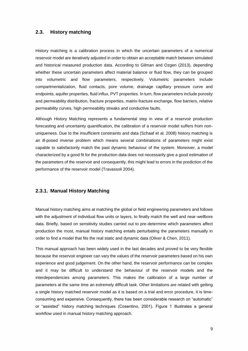
or “assisted” history matching techniques (Cosentino, 2001). Figure 1 illustrates a general
workflow used in manual history matching approach.
10
Figure 1 - General workflow in manual history matching.
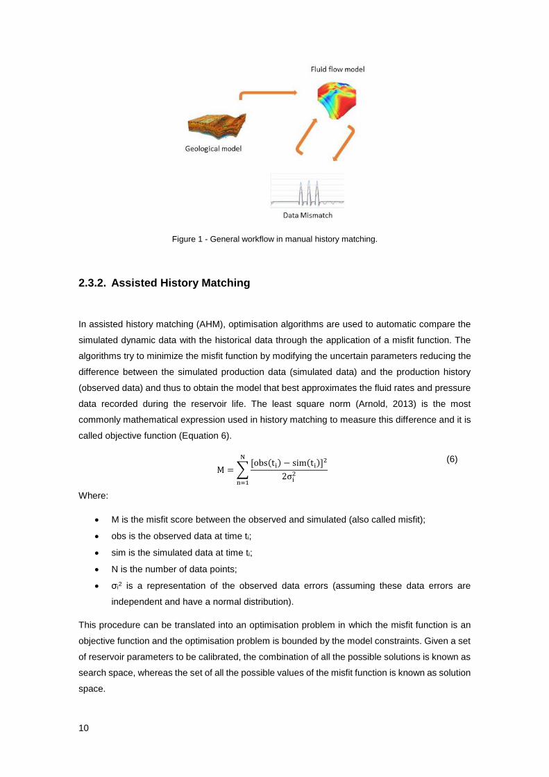
2.3.2. Assisted History Matching
In assisted history matching (AHM), optimisation algorithms are used to automatic compare the
simulated dynamic data with the historical data through the application of a misfit function. The
algorithms try to minimize the misfit function by modifying the uncertain parameters reducing the
difference between the simulated production data (simulated data) and the production history
(observed data) and thus to obtain the model that best approximates the fluid rates and pressure
data recorded during the reservoir life. The least square norm (Arnold, 2013) is the most
commonly mathematical expression used in history matching to measure this difference and it is
called objective function (Equation 6).
M = ∑
[obs(ti) − sim(ti)]2
2σi2
N
n=1
(6)
Where:
• M is the misfit score between the observed and simulated (also called misfit);
• obs is the observed data at time ti;
• sim is the simulated data at time ti;
• N is the number of data points;
• σi2 is a representation of the observed data errors (assuming these data errors are
independent and have a normal distribution).
This procedure can be translated into an optimisation problem in which the misfit function is an
objective function and the optimisation problem is bounded by the model constraints. Given a set
of reservoir parameters to be calibrated, the combination of all the possible solutions is known as
search space, whereas the set of all the possible values of the misfit function is known as solution
space.

11
Several of the AHM techniques are used today in the industry. The methods based on heuristic
optimisers or direct search, have the advantage of leading to multiple calibrated models that
partially address the problem of the non-uniqueness of the solutions (Ferraro and Verga, 2009).
A general workflow used in assisted history matching is illustrated in Figure 2.
Figure 2 - General workflow in assisted history matching.
2.4. Optimisation algorithms
In assisted history matching, the model output parameters are modified in order to minimize the
difference between the model result and the actual field data. The minimization process is referred
to as optimisation process and a number of optimisation techniques have been proposed. The
most common approaches use gradient methods, data assimilation methods and stochastic
search algorithms.
Gradient optimisation has been widely used to optimise objective functions. The gradient
optimisation techniques include the Steepest descent, Conjugate gradient, Gauss-Newton, and
Dog-leg techniques. The gradient method involves calculation of the objective function gradient
with respect to model input parameter. Although it is a fast and easy method for implementation,
it has some limitations as there is the possibility of getting trapped in local minima far from the
global one and it is a non-linear optimisation algorithm that relies on a single model for
perturbation (Christie et al, 2005).
The data-assimilation optimisation can be separated into an analysis (or update) step and a
forecast step. At the analysis step, an improved estimate of model variables is obtained by
applying Bayes’ theorem to compute the posterior probability density function (PDF) for the model
variables given the observations. At the forecast step, the dynamical model is advanced in time
and its result becomes the forecast (or prior) in the next analysis cycle (Christie et al, 2005).
Ensemble Kalman Filter (EnKF) is a data assimilation technique that has gained increasing
interest in the application of petroleum history matching in recent years. The basic methodology
12
of the EnKF consists of the forecast step and the update step. This data assimilation method
utilises a collection of state vectors, known as an ensemble, which are simulated forward in time
(Christie et al, 2005). In other words, each ensemble member represents a reservoir model.
Subsequently, during the update step, the sample covariance is computed from the ensemble,
while the collection of state vectors is updated using the formulations which involve this updated
sample covariance.
The Stochastic Optimisation is considered in a subsection as it is used under the scope of this
thesis.
2.4.1. Stochastic Optimisation
Adaptive Stochastic Sampling algorithms are population-based optimisation algorithms inspired
by process occurring in biological evolution and the most commonly used are Genetic algorithms
(Erbas & Christie, 2007), Simulated Annealing (Ingber, 1993), Evolutionary algorithms (Schulze-
Riegert et al., 2001) and Swarm algorithms (Mohamed et al., 2010).
Population-based systems are composed of multiple intelligent individuals that improve the quality
of solutions by interpreting the interactions among members. While searching for optimal
solutions, these kinds of methods also provide the opportunity to balance exploration and
exploitation. Exploration is defined as the search for different areas in the parameter space while
exploitation refers to the refinement of the previously visited regions to find better answers. The
most recent stochastic algorithms are the evolutionary and swarm algorithms which have the
ability not to get trapped in local minima so often and therefore achieve better results when
quantifying uncertainty (Hajizadeh et al., 2011).
Particle Swarm Optimisation
The Particle Swarm Optimisation (PSO) was developed by Kennedy and Eberhart (1995). It was
initially designed to measure the social behaviour of a group of birds but its application has been
extended to various fields including petroleum engineering (Hajizadeh et al., 2010). The basic
principle behind the algorithm is that birds belonging to a particular flock would generally tend to
fly towards regions perceived to exhibit certain habitat characteristics at a particular point in time.
Each member of the flock thus has a memory of its best historical location and the flock is often
characterized by a global best position. The Particle Swarm Optimisation process involves
initiating a swarm of particles which randomly search the sample space in an attempt to obtain a
sufficient solution to a particular objective function. This algorithm can be applied both in a single
and multi-objective optimisation. When compared to the single objective, the multi-objective
13
approach of the PSO algorithm presents an improvement in model diversity and is characterized
by more efficiency in estimating the uncertainty due to a faster convergence speed (Mohamed et
al., 2011).
The basic workflow for the PSO may be summarised:
1) Initialise the particle swarm (i.e. distribute specified number of particles randomly in
sample space);
2) Evaluate the objective function for each particle in the swarm;
3) Compare each particle’s fitness value with that corresponding to its best position (pbest).
Replace pbest with the current position if the current value of the fitness function is less
than that corresponding to pbest;
4) Update the global best position and fitness value of the swarm;
5) Update the velocities and positions of each particle.
This process is repeated until a stopping criteria is reached.
2.4.2. Single Objective vs Multi-Objective Optimisation
The principle of a single objective optimisation is different from that in a multi-criteria optimisation.
In single objective optimisation, the goal is to find the best solution, which corresponds to the
minimum or maximum value of the objective function (Ferraro & Verga, 2009). This means that
the algorithm uses a single match quality number in searching for better solutions. The single
objective approach sums up all the misfit components using equation 6, presented in section
2.3.2.
On the contrary, in a multi-criteria optimisation more than one objective is defined, there is no
single optimal solution and at least one criteria is verified. The presence of more than one
objective (conflicting objectives) makes these objectives to trade-off between each other and so,
the improvement in one objective may cause deterioration in another (Ferraro & Verga, 2009).
Therefore, it is essential to find solutions that balance these trade-offs, the so called non-
dominated solutions, which means solutions that cannot improve any objective without degrading
one or more of the other objectives (Mohamed et al, 2011).
As in a multi-objective optimisation the misfit function is split into several components which are
optimised simultaneously, the objective function takes the vector form (Mohamed et al, 2011):
F(x) = [f1(x), … , fM(x)] (7)
Where:
• fi, i=1,…, M are the objective functions.
14
The formulation of a multi-objective optimisation process is to minimize F(x) subject to:
hkl ≤ xk ≤ hk
u (8)
x = {x1, x2, … , xk, … , xN} (9)
Where:
• F(x): RN RM, x={x1,x2,…,xk,…,xN} is the vector of the N variables in the
parameterisation;
• hkl and hk
u represent the lower and upper boundary for each unknown, respectively.
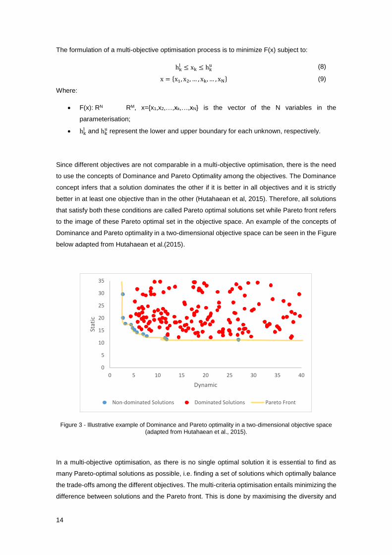
Since different objectives are not comparable in a multi-objective optimisation, there is the need
to use the concepts of Dominance and Pareto Optimality among the objectives. The Dominance
concept infers that a solution dominates the other if it is better in all objectives and it is strictly
better in at least one objective than in the other (Hutahaean et al, 2015). Therefore, all solutions
that satisfy both these conditions are called Pareto optimal solutions set while Pareto front refers
to the image of these Pareto optimal set in the objective space. An example of the concepts of
Dominance and Pareto optimality in a two-dimensional objective space can be seen in the Figure
below adapted from Hutahaean et al.(2015).
Figure 3 - Illustrative example of Dominance and Pareto optimality in a two-dimensional objective space
(adapted from Hutahaean et al., 2015).
In a multi-objective optimisation, as there is no single optimal solution it is essential to find as
many Pareto-optimal solutions as possible, i.e. finding a set of solutions which optimally balance
the trade-offs among the different objectives. The multi-criteria optimisation entails minimizing the
difference between solutions and the Pareto front. This is done by maximising the diversity and
0
5
10
15
20
25
30
35
0 5 10 15 20 25 30 35 40
Stat
ic
Dynamic
Non-dominated Solutions Dominated Solutions Pareto Front
15
spread of the non-dominated solutions to represent as much as possible of the Pareto front while
maximizing the number of elements of the Pareto optimal set found maintaining the ones which
were already found (Mohamed et al, 2011).
The MOO was already used in history matching and some of these approaches implemented in
different optimisation algorithms have been reported in the literature.
The first application of MOO in HM was implemented by Schulze-Riegert et al. (2007) where they
address the problem of multi-objective criteria in a history match study and present analysis
techniques identifying competing match criteria by discussing a Pareto-Optimiser.
Ferraro and Verga (2009) employed a genetic algorithm and evolutionary strategies with different
parameter combinations in both single and multi-objective optimisation techniques. Their study
demonstrated that the application of a multi-objective approach improves the history matching
regarding the convergence rate and the distance from the real solution. Additionally, since it is
possible to find multiple conflicting objective functions, a range of equally likely scenarios can also
be obtained.
Hajidazeh et al. (2011) used a multi-objective stochastic population-based optimisation for history
matching and uncertainty quantification of a synthetic case. Multi-objective differential evolution
as shown faster convergence, better final misfit value during history matching and obtained stable
Bayesian credible intervals in fewer simulations when compared with the objective sum approach
using the standard DE.
Mohamed et al. (2011) compared the results between a single objective methodology and the
multi-objective particle swarm optimisation scheme on history matching a synthetic reservoir
simulation model. They concluded that the multi-objective particle swarm approach is highly
competitive in obtaining a well distributed set of good fitting reservoir models. This approach
obtained the models faster and with similar quality, providing a more accurate estimation of
uncertainty in predictions in comparison to the single objective approach.
Christie et al. (2013) compared the performance of both single and multi-objective versions of the
Particle Swarm Optimisation algorithm for history matching a real field. Multi-objective matching
proved to increase not only the speed in matching but also a diversity in the models found that
produce the same low misfits as in the single objective matching.
Hutahaean et al. (2015) explore the impact of different geological model parameterisations on
AHM by comparing the performance of SO and MO AHM approaches. They concluded that under
different model parameterisations the MO AHM approach results in a more diverse set of models
leading to a more robust and more reliable forecast than the one from SO approach.

16
2.5. Uncertainty Assessment
The current trend for history match workflows is to find multiple matched models instead of a
single set of model parameters that match the data. The importance of achieving multiple
solutions is that they can be used for uncertainty quantification of the production forecast.
It is important to produce a set of models that match the production data consistent with the known
prior information allowing the quantification of the uncertainty. Through the generation of multiple
history matched models it is possible not only to quantify the probability of future production but
also to identify what scenario is the most likely and what are the respective confidence intervals.
2.5.1. Bayesian Framework and Uncertainty Quantification
Bayesian inference is based on the Bayes’ theorem and used to perform inferences about the
value of some parameters based on prior and newly observed information. Bayes’ Theorem is
represented by Equation 10.
P(m|Ο) =
P(O|m) P(m)
∫ P(O|m)P(m)dmM
(10)
Where:
• P(m|O) is the posterior probability of the model;
• P(O|m) is the data likelihood;
• p(m) is the initial prior probability distribution;
• M is the space of the model.
Likelihood of a reservoir model can be defined as the probability that reservoir observation data
is equal to simulation responses based on a specific reservoir model. The likelihood is
represented by Equation 11.
p(O|m) = e−M (11)
Where:
• M is the misfit as calculated following for example equation 6.
The Posterior Probability Distribution (PPD) or p(m|O) represents the updated knowledge about
the model m based on the observations O and the prior knowledge of the model. It can be
calculated using the Neighbourhood Algorithm-Bayes (NAB; Sambridge, 1999) which is based on
Markov Chain Monte Carlo.NAB uses Voronoi cells to interpolate values of misfit away from the

17
known sampled points (models in the parameter space), for which the likelihood is computed
exactly, and a Gibbs sampler to estimate the PPD (Christie, 2006). The resulting ensemble of the
model with their posterior probabilities can be used to estimate the P10 – P50 – P90 confidence
interval to describe the uncertainty envelopes for reservoir performance.
2.5.2. Bayesian Model Averaging
Bayesian Model Averaging (BMA) was first applied in weather forecasting and its success made
it to be applied in other study areas such as oil production forecasting (Raftery et al., 2005).
It is a technique applied with the purpose of combining the probability distribution functions (PDF)
from different models into a single PDF (Figure 4). The combination of the different PDF
encompasses a weighted average of the individual forecast based on the uncertainty forecast
and variance between models.
Figure 4 - BMA PDF (thick curve) based on 5 models (thin curves) (adapted from Raftery et al. 2005).
BMA PDF of a quantity y based on K models is given by:
p(y|f1, … , fK) = ∑ wK
K
K=1
gK(y|fK) (12)
Where:
• fk is the forecasting of model k
• wk is the posterior weight of model k
• gk(y|fk) is the PDF of y given the forecast fk

18
Assuming a normal distribution (Raftery et al., 2005), the BMA mean (E) is represent by:
E(y|f1, … , fK) = ∑ wK
K
K=1
fK (13)
The posterior weights, wk, are calculated using:
wK =
Bkj
∑ Bijki=1
(14)
where Bkj is the Bayes Factor of model k regarding the assumed best model j (maximum
likelihood).
Bayes Factor assumes independent conditional distributions and allows to compare the validity
of the different models according to their data Bayes Factor of model k (mk) regarding model j
(mj), Bkj, can be calculated recurring to Laplace’s Method (Kass and Raftery, 1995):
Bkj =
p(Õ|mk)
p(Õ|mj)
(15)
where p(O|mx) is the posterior probability of model x around the maximum likelihood model.
BMA is used in this thesis to estimate the cumulative oil and water uncertainty envelopes by
combining the uncertainty envelopes associated with the different model parameterisations.
19
3. Methodology
This project entails the development of a multi-objective optimisation (MOO) stochastic history
matching technique able to match simultaneously static and dynamic data. This procedure was
implemented in the PUNQ-S3 benchmark reservoir.
In this reservoir, matching exclusively the production data (Gas-Oil Ratio, Borehole Pressure and
Water Cut) allows retrieving an ensemble of history matched models able to reproduce the
historical production data for these three production variables. Despite the results, when
comparing the optimised static models of porosity, horizontal permeability and vertical
permeability against the truth case at the well locations, large differences between the values are
identified.
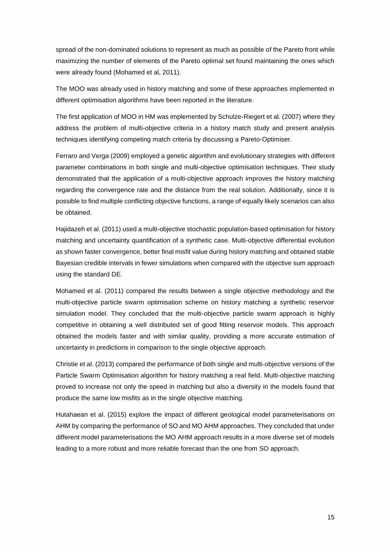
The solution proposed to overcome this drawback is to pose history match as a multi-objective
problem minimizing simultaneously an objective composed by the differences between real and
optimised static data and another with the difference between observed and simulated production
data. A Multi-Objective Optimisation approach is applied and the models belonging to the Pareto
fronts are studied to make a balance of the trade-offs between the objective with the difference in
the static data and the objective with the difference in the production data. The workflow for the
proposed methodology is illustrated in Figure 5.
Figure 5 - Workflow for the methodology applied in this thesis.
20
The proposed multi-objective history matching methodology may be summarized in the following
sequence of steps:
1 – Definition of the parameterisation of the geological model;
2 – Optimisation of the geological parameters of the model using the MOPSO algorithm (section
2.4.1);
3 – Introduction of the optimised petrophysical properties in the static objective for minimization;
4 – Run a flow simulator to obtain the dynamic response of the optimised model;
5 – Introduction of the simulated dynamic response in the dynamic objective for minimization;
6 – Minimization of both objectives and identification of the models (Pareto Models) that best
approximate both petrophysical properties and dynamic response to the truth case (sections 2.3.2
and 2.4.2);
This process is repeated until a stopping criteria is reached which in this case is the maximum
number of iterations.
7 – Characterization and quantification of the uncertainty of predictions of the ensemble of history
matched models recurring to the Neighbourhood Algorithm-Bayes algorithm (section 2.5.1).
The Bayesian Model Averaging was then applied to combine the forecast for the different model
parameterisations and obtain a single forecast model (section 2.5.2).
In order to evaluate the performance and ability of the proposed MOO technique in both history
matching and uncertainty characterization of predictions, a multi-objective optimisation approach
for history matching was applied to the different model parameterisations considering two
objective functions as described by the match between observed and simulated production data
for the dynamic properties under study. The scheme of objective grouping used in this approach
was adopted from previous study (Hutahaean et al., 2015) in which the wells are grouped based
on geo-engineering judgement in the reservoir model studied.
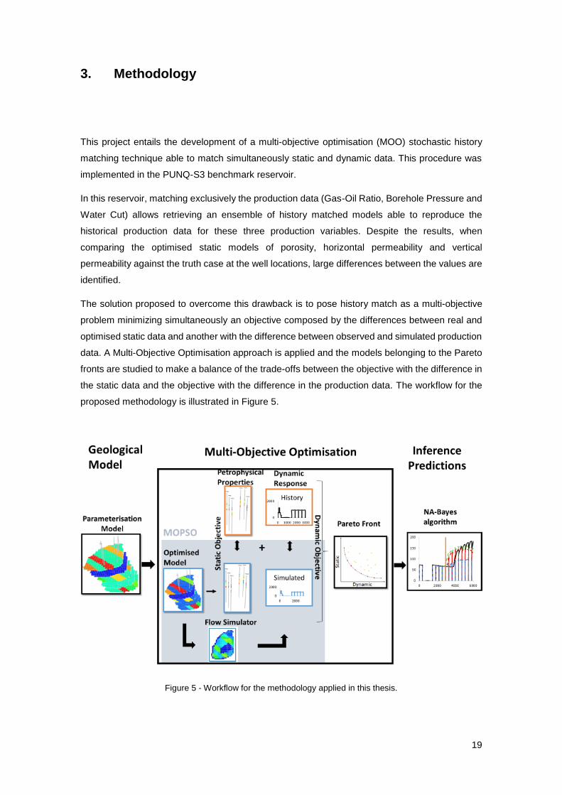
The workflow for history matching exclusively the model to dynamic data can be seen in Figure
6.
After optimising the geological parameters (section 2.4.1) and obtaining the dynamic response of
the model from a flow simulator, the algorithm minimizes the misfit function (section 2.4.2) and
consequently identifies the reservoir model that best approximates its dynamic response to the
historical production behaviour of the field (section 2.3.2). The uncertainty of predictions of the
ensemble of history matched models is then characterized and quantified using the
Neighbourhood Algorithm-Bayes algorithm (Section 2.5.1).
The history matching procedure is done by Epistemy’s Raven, which is an assisted history
matching software using a multi-objective optimisation approach powered by the Particle Swarm
21
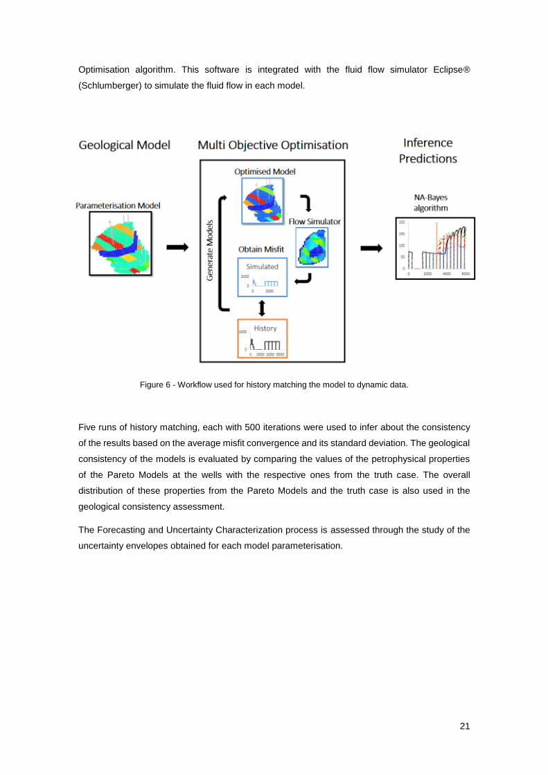
Optimisation algorithm. This software is integrated with the fluid flow simulator Eclipse®
(Schlumberger) to simulate the fluid flow in each model.
Figure 6 - Workflow used for history matching the model to dynamic data.
Five runs of history matching, each with 500 iterations were used to infer about the consistency
of the results based on the average misfit convergence and its standard deviation. The geological
consistency of the models is evaluated by comparing the values of the petrophysical properties
of the Pareto Models at the wells with the respective ones from the truth case. The overall
distribution of these properties from the Pareto Models and the truth case is also used in the
geological consistency assessment.
The Forecasting and Uncertainty Characterization process is assessed through the study of the
uncertainty envelopes obtained for each model parameterisation.

22
This page intentionally left blank
23
4. Application example
This chapter comprises the description of the benchmark synthetic dataset after which are
presented the results of the methodologies applied under the scope of this thesis and its
discussion.
4.1. PUNQ-S3 Field description
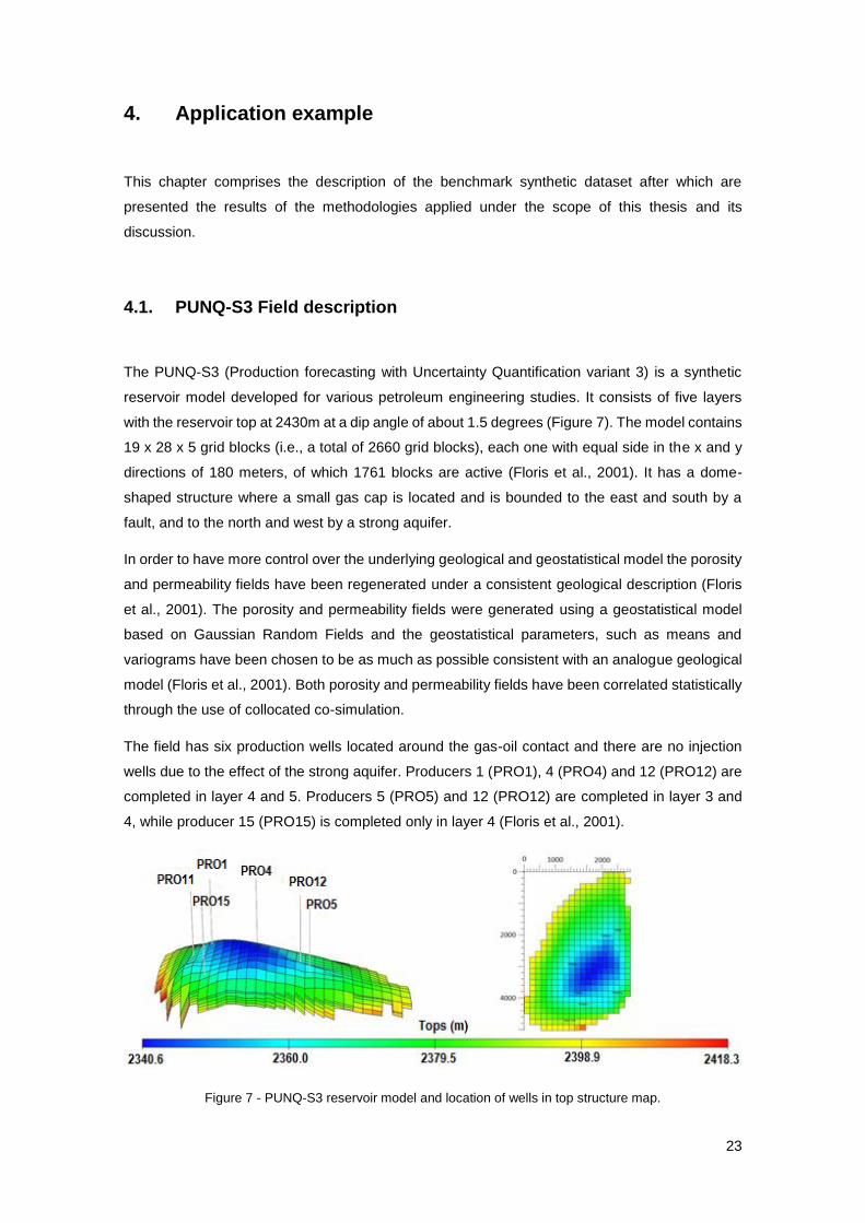
The PUNQ-S3 (Production forecasting with Uncertainty Quantification variant 3) is a synthetic
reservoir model developed for various petroleum engineering studies. It consists of five layers
with the reservoir top at 2430m at a dip angle of about 1.5 degrees (Figure 7). The model contains
19 x 28 x 5 grid blocks (i.e., a total of 2660 grid blocks), each one with equal side in the x and y
directions of 180 meters, of which 1761 blocks are active (Floris et al., 2001). It has a dome-
shaped structure where a small gas cap is located and is bounded to the east and south by a
fault, and to the north and west by a strong aquifer.
In order to have more control over the underlying geological and geostatistical model the porosity
and permeability fields have been regenerated under a consistent geological description (Floris
et al., 2001). The porosity and permeability fields were generated using a geostatistical model
based on Gaussian Random Fields and the geostatistical parameters, such as means and
variograms have been chosen to be as much as possible consistent with an analogue geological
model (Floris et al., 2001). Both porosity and permeability fields have been correlated statistically
through the use of collocated co-simulation.
The field has six production wells located around the gas-oil contact and there are no injection
wells due to the effect of the strong aquifer. Producers 1 (PRO1), 4 (PRO4) and 12 (PRO12) are
completed in layer 4 and 5. Producers 5 (PRO5) and 12 (PRO12) are completed in layer 3 and
4, while producer 15 (PRO15) is completed only in layer 4 (Floris et al., 2001).
Figure 7 - PUNQ-S3 reservoir model and location of wells in top structure map.
24
The production history of the six wells is characterized by an extended well testing period (build
up test) during the first year, a shut-in period for the next three years and a production period for
the next 12 years with fixed oil production rate at 150 std m3/d and a 2 week periodic shut-in at
the beginning of each year. For history matching the model, eight years of production history data
which includes gas-oil ratio (WGOR), water cut (WWCT) and borehole pressure (WBHP), are
used (Floris et al., 2001). As the available production of the field lasts for 16.5 years, the following
8.5 years were used exclusively to evaluate the predictive ability of the history matched models
in terms of production forecasting (Floris et al., 2001).
4.2. Geological description
The original description of PUNQ-S3 (Floris et al. 2001) does not provide an exhaustive
description of the geological background used to generate the dataset. Therefore, under the
scope of this work, the background geology was modelled by relying in analogue fields. According
to Floris et al. (2001), the sediments in this reservoir model were deposited in a deltaic coastal
plain environment.
The following subsections describe this type of environment as well as its typical deposits and
facies.
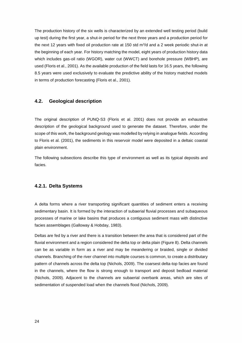
4.2.1. Delta Systems
A delta forms where a river transporting significant quantities of sediment enters a receiving
sedimentary basin. It is formed by the interaction of subaerial fluvial processes and subaqueous
processes of marine or lake basins that produces a contiguous sediment mass with distinctive
facies assemblages (Galloway & Hobday, 1983).
Deltas are fed by a river and there is a transition between the area that is considered part of the
fluvial environment and a region considered the delta top or delta plain (Figure 8). Delta channels
can be as variable in form as a river and may be meandering or braided, single or divided
channels. Branching of the river channel into multiple courses is common, to create a distributary
pattern of channels across the delta top (Nichols, 2009). The coarsest delta-top facies are found
in the channels, where the flow is strong enough to transport and deposit bedload material
(Nichols, 2009). Adjacent to the channels are subaerial overbank areas, which are sites of
sedimentation of suspended load when the channels flood (Nichols, 2009).
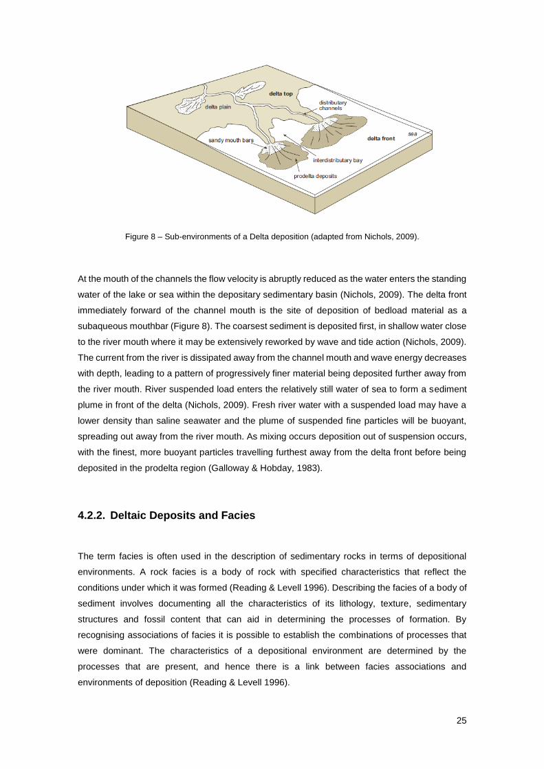
25
Figure 8 – Sub-environments of a Delta deposition (adapted from Nichols, 2009).
At the mouth of the channels the flow velocity is abruptly reduced as the water enters the standing
water of the lake or sea within the depositary sedimentary basin (Nichols, 2009). The delta front
immediately forward of the channel mouth is the site of deposition of bedload material as a
subaqueous mouthbar (Figure 8). The coarsest sediment is deposited first, in shallow water close
to the river mouth where it may be extensively reworked by wave and tide action (Nichols, 2009).
The current from the river is dissipated away from the channel mouth and wave energy decreases
with depth, leading to a pattern of progressively finer material being deposited further away from
the river mouth. River suspended load enters the relatively still water of sea to form a sediment
plume in front of the delta (Nichols, 2009). Fresh river water with a suspended load may have a
lower density than saline seawater and the plume of suspended fine particles will be buoyant,
spreading out away from the river mouth. As mixing occurs deposition out of suspension occurs,
with the finest, more buoyant particles travelling furthest away from the delta front before being
deposited in the prodelta region (Galloway & Hobday, 1983).
4.2.2. Deltaic Deposits and Facies
The term facies is often used in the description of sedimentary rocks in terms of depositional
environments. A rock facies is a body of rock with specified characteristics that reflect the
conditions under which it was formed (Reading & Levell 1996). Describing the facies of a body of
sediment involves documenting all the characteristics of its lithology, texture, sedimentary
structures and fossil content that can aid in determining the processes of formation. By
recognising associations of facies it is possible to establish the combinations of processes that
were dominant. The characteristics of a depositional environment are determined by the
processes that are present, and hence there is a link between facies associations and
environments of deposition (Reading & Levell 1996).

26
A key feature of many deltas is the close association of marine and continental depositional
environments. In delta deposits this association is seen in the vertical arrangement of facies. A
single delta cycle may show a continuous vertical transition from fully marine conditions at the
base to a subaerial setting at the top (Nichols, 2009). This transition is typically within a coarsening
upwards succession from lower energy, finer grained deposits of the prodelta to the higher energy
conditions of the delta mouth bar where coarser sediment accumulates (Nichols, 2009).
The delta top contains both relatively coarse sediment of the distributary channel as well as finer
grained material in overbank areas and interdistributary bays (Galloway & Hobday, 1983). The
channel may be recognised by its scoured base, a fining-up pattern and evidence of flow. Fluvial
channel fills (Figure 9(a)) is the typical facies found in channels and consists of interbedded fine
sand, silt, and some mud, in which resultant units are lenticular and nearly symmetrical
(Galloway& Hobday, 1983).
Figure 9 - Example of fluvial channel fills (a) and floodplain mudstone (b) facies types (Grundvag et al., 2014).
Deposits in the sheltered interdistributary bays may show thin bedding resulting from influxes of
sediment from the delta top. According to Galloway & Hobday (1983) the facies type formed
usually consist of natural levee deposits of massive to interbedded silt and mud, marsh and
swamp peat, organic-rich clay and mud, and lacustrine mud and clay, resembling comparable to
floodplain settings (Figure 9(b)).
The shallower water deposits of the delta front may be extensively reworked by wave and/or tidal
action resulting in cross-stratified mouth-bar facies (Figure 10(a)). Mouthbar is characterized by
sands and associated silts and muds containing abundant macerated plant debris as well as large
chunks of woody material (Galloway & Hobday, 1983). Thin, discontinuous mud drapes and
pockets of reworked mud clasts reflect the variability of fluvial scour and deposition. Laterally,
mouthbar deposits grade into interdistributary sand, silt, mud and clay, and may be overlain by
crevasse-splay sequences (Figure 10(b)).
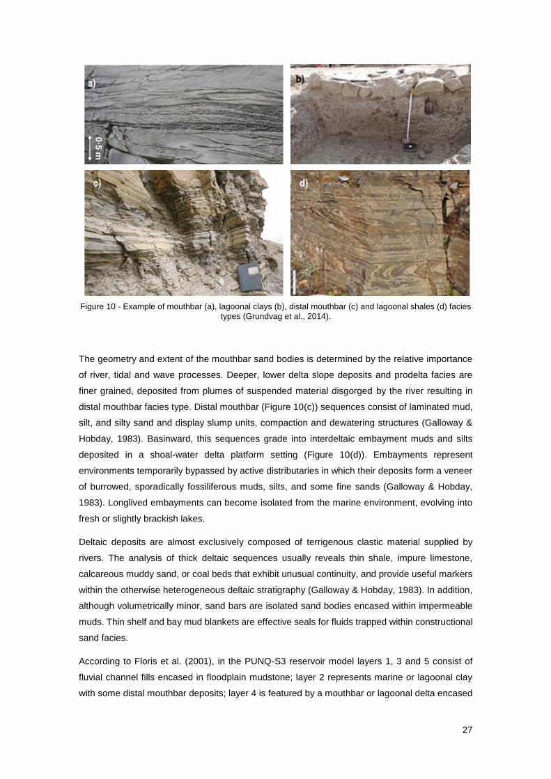
27
Figure 10 - Example of mouthbar (a), lagoonal clays (b), distal mouthbar (c) and lagoonal shales (d) facies
types (Grundvag et al., 2014).
The geometry and extent of the mouthbar sand bodies is determined by the relative importance
of river, tidal and wave processes. Deeper, lower delta slope deposits and prodelta facies are
finer grained, deposited from plumes of suspended material disgorged by the river resulting in
distal mouthbar facies type. Distal mouthbar (Figure 10(c)) sequences consist of laminated mud,
silt, and silty sand and display slump units, compaction and dewatering structures (Galloway &
Hobday, 1983). Basinward, this sequences grade into interdeltaic embayment muds and silts
deposited in a shoal-water delta platform setting (Figure 10(d)). Embayments represent
environments temporarily bypassed by active distributaries in which their deposits form a veneer
of burrowed, sporadically fossiliferous muds, silts, and some fine sands (Galloway & Hobday,
1983). Longlived embayments can become isolated from the marine environment, evolving into
fresh or slightly brackish lakes.
Deltaic deposits are almost exclusively composed of terrigenous clastic material supplied by
rivers. The analysis of thick deltaic sequences usually reveals thin shale, impure limestone,
calcareous muddy sand, or coal beds that exhibit unusual continuity, and provide useful markers
within the otherwise heterogeneous deltaic stratigraphy (Galloway & Hobday, 1983). In addition,
although volumetrically minor, sand bars are isolated sand bodies encased within impermeable
muds. Thin shelf and bay mud blankets are effective seals for fluids trapped within constructional
sand facies.
According to Floris et al. (2001), in the PUNQ-S3 reservoir model layers 1, 3 and 5 consist of
fluvial channel fills encased in floodplain mudstone; layer 2 represents marine or lagoonal clay
with some distal mouthbar deposits; layer 4 is featured by a mouthbar or lagoonal delta encased
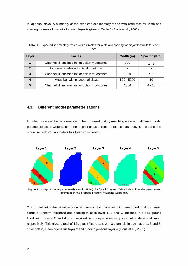
28
in lagoonal clays. A summary of the expected sedimentary facies with estimates for width and
spacing for major flow units for each layer is given in Table 1 (Floris et al., 2001).
Table 1 - Expected sedimentary facies with estimates for width and spacing for major flow units for each layer.
Layer Facies Width (m) Spacing (Km)
1 Channel fill encased in floodplain mudstones 800 2 - 5
2 Lagoonal shales with distal mouthbar - -
3 Channel fill encased in floodplain mudstones 1000 2 - 5
4 Mouthbar within lagoonal clays 500 - 5000 10
5 Channel fill encased in floodplain mudstones 2000 4 - 10
4.3. Different model parameterisations
In order to assess the performance of the proposed history matching approach, different model
parameterisations were tested. The original dataset from the benchmark study is used and one
model set with 24 parameters has been considered.
Layer 1 Layer 2 Layer 3 Layer 4 Layer 5
Figure 11 - Map of model parameterisation in PUNQ-S3 for all 5 layers. Table 2 describes the parameters
optimised in the proposed history matching approach.
This model set is described as a deltaic coastal plain reservoir with three good quality channel
sands of uniform thickness and spacing in each layer 1, 3 and 5, encased in a background
floodplain. Layers 2 and 4 are classified in a single zone as poor-quality shale and sand,
respectively. This gives a total of 12 zones (Figure 11), with 3 channels in each layer 1, 3 and 5,
1 floodplain, 1 homogeneous layer 2 and 1 homogeneous layer 4 (Floris et al., 2001).

29
Each zone has a corresponding parameter for porosity and another for horizontal permeability
multiplier, resulting in a total of 24 parameters, 12 for porosity and 12 for horizontal permeability
multipliers (Table 2; Floris et al., 2001).
Table 2 - Parameter corresponding to each zone of the model.
Zone Porosity
Parameter
Horizontal Permeability
Multiplier Parameter
Layer 1
Channel a $pa1 $Multipa1
Channel b $pb1 $Multipb1
Channel c $pb3 $Multipc1
Background floodplain $pbackground $Multipbackground
Homogeneous layer 2 $p2 $Multip2
Layer 3
Channel a $pa3 $Multipa3
Channel b $pb3 $Multipb3
Channel c $pc3 $Multipc3
Homogeneous layer 4 $p4 $Multip4
Layer 5
Channel a $pa5 $Multipa5
Channel b $pb5 $Multipb5
Channel c $pc5 $Multipc5
This model set is characterized by some geological inconsistencies namely in layers 2, 4 and 5.
While in the truth case layers 2 and 4 are featured by two different facies types, in the model the
same layers are described has homogeneous regions and so, have no ability to encompass the
uncertainty associated with the different geological facies. The analysis of deltaic depositional
sequences from analogue reservoirs also allows to infer that mouthbar facies type is usually found
near the upper parts of the vertical sequence of facies rather than being deposited in the fourth
layer. Regarding layer 5, although it is featured with three channels, they are placed next to each
other which is neither geologically consistent or coherent with the truth case.
Three different model parameterisations were used for comparison and are described in the
following subsections.
4.3.1. Parameterisation A
The results obtained in history matching model parameterisation A were the basis for stimulating
the implementation of the proposed MOO methodology for reservoir history matching. The
30
problem in history matching the PUNQ-S3 reservoir only to production variables was identified
through the analysis of the results from this model parameterisation.
Model Parameterisation A is based on the geological facies description of PUNQ-S3 to define the
porosity range for each zone (Table 3). Although based on the geological facies description, the
prior ranges for the different petrophysical properties were not set considering the prior
distributions from the truth case (TC).
In this model parameterisation, horizontal and vertical permeabilities are correlated from porosity
values obtained based on least square fitting of well data crossplots, using Equations 16 and 17.
Table 3 - Porosity ranges of different facies used in model parameterisation A.
Zone Porosity range (fraction) Horizontal permeability
range (mD)
Channels (layer 1, 3 ,5) 0.15 – 0.30 13 - 30000
Background floodplain 0.05 – 0.15 1.5 – 1330
Homogeneous layer (2 and 4) 0.05 – 0.15 1.5 - 1330
ln(Kh) = ln(Mult) + (0.77 + 9.03∅) (16)
Kv = 3.124 + 0.306Kh (17)
The calculation of Kh from Ø leads to errors which are compensated using multipliers as variable
parameters and then the vertical permeability is calculated from horizontal permeability.
This model parameterisation was only used to history match to the production data using the
workflow described in section 3 for history matching the model to dynamic data.
4.2.2. Parameterisation B
Model parameterisation B was history matched using the proposed methodology to obtain the
match for both static and dynamic data.
With the purpose of improving the geological consistency of the model, the prior distributions of
the parameters were modified based not only in the distributions of the TC but also in the range
in which porosity and permeability vary between wells within the same zones of the model. The
ranges in which porosity and horizontal permeability vary are in Table 4. The correlation between
porosity and both permeabilities is the same used in model Parameterisation A (Equations 16 and
17).
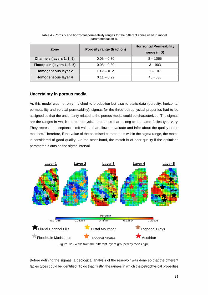
31
Table 4 - Porosity and horizontal permeability ranges for the different zones used in model parameterisation B.
Zone Porosity range (fraction) Horizontal Permeability
range (mD)
Channels (layers 1, 3, 5) 0.05 – 0.30 8 – 1065
Floodplain (layers 1, 3, 5) 0.08 – 0.30 3 – 903
Homogeneous layer 2 0.03 – 012 1 – 107
Homogeneous layer 4 0.11 – 0.22 40 - 630
Uncertainty in porous media
As this model was not only matched to production but also to static data (porosity, horizontal
permeability and vertical permeability), sigmas for the three petrophysical properties had to be
assigned so that the uncertainty related to the porous media could be characterized. The sigmas
are the ranges in which the petrophysical properties that belong to the same facies type vary.
They represent acceptance limit values that allow to evaluate and infer about the quality of the
matches. Therefore, if the value of the optimised parameter is within the sigma range, the match
is considered of good quality. On the other hand, the match is of poor quality if the optimised
parameter is outside the sigma interval.
Layer 1 Layer 2 Layer 3 Layer 4 Layer 5
Fluvial Channel Fills Distal Mouthbar Lagoonal Clays
Floodplain Mudstones Lagoonal Shales Mouthbar
Figure 12 - Wells from the different layers grouped by facies type.
Before defining the sigmas, a geological analysis of the reservoir was done so that the different
facies types could be identified. To do that, firstly, the ranges in which the petrophysical properties

32
vary in each layer were identified and then these properties at all wells were plotted. The regions
where the wells are placed in the TC were also taken into account. Considering these values and
the description of analogue depositional environments and facies (Galloway & Hobday, 1983;
Barwis et al., 1990; Reading & Levell 1996; Nichols, 2009; Grundvag et al., 2014), the facies
types were defined. This analysis leaded to the identification of 6 different facies and the wells
belonging to the same facies type were grouped (Figure 12).
After grouping the wells by facies type, the variation between their petrophysical properties was
studied. Considering this variation as well as the geological characteristics of each facies, the
sigmas were assigned to make a distinction between the facies with good capacity for the fluids
to flow, storage hydrocarbons and the ones which have an impermeable behaviour. Therefore,
larger sigmas were assigned to the petrophysical properties from fluvial channel fills and
mouthbar facies types than the ones from floodplain mudstones, lagoonal shales, distal mouthbar
and lagoonal clays facies types. The sigmas assigned to each petrophysical property from the
different facies types in model B are shown in Table 5.
Table 5 - Sigmas assigned to the petrophysical properties (porosity, horizontal permeability and vertical
permeability) for the different facies types.
Petrophysical
Property
Facies Type
Fluvial
Channel
Floodplain
Mudstones
Lagoonal
Shales
Distal
Mouthbar Mouthbar
Lagoonal
Clays
Porosity
(fraction) 0.1 0.03 0.01 0.02 0.05 0.02
Horizontal
Permeability
(mD)
200 20 10 20 160 60
Vertical
Permeability
(mD)
100 10 4 10 40 20
For terms of comparison, model B was used for history matching to static and dynamic data (B
Sta&Dyn) as well as only to dynamic data (B Dyn).
4.2.3. Parameterisation C
In model parameterisation C not only the facies, prior distributions and sigmas were adjusted but
also a new zone orientation was tested. There was the need to test a different zone orientation
as the zonation of the original model is not geologically coherent with the truth case. This lack of
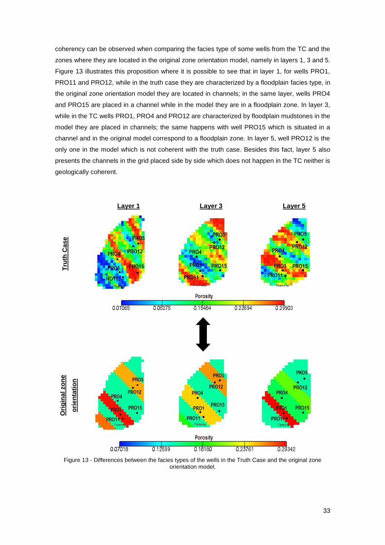
33
coherency can be observed when comparing the facies type of some wells from the TC and the
zones where they are located in the original zone orientation model, namely in layers 1, 3 and 5.
Figure 13 illustrates this proposition where it is possible to see that in layer 1, for wells PRO1,
PRO11 and PRO12, while in the truth case they are characterized by a floodplain facies type, in
the original zone orientation model they are located in channels; in the same layer, wells PRO4
and PRO15 are placed in a channel while in the model they are in a floodplain zone. In layer 3,
while in the TC wells PRO1, PRO4 and PRO12 are characterized by floodplain mudstones in the
model they are placed in channels; the same happens with well PRO15 which is situated in a
channel and in the original model correspond to a floodplain zone. In layer 5, well PRO12 is the
only one in the model which is not coherent with the truth case. Besides this fact, layer 5 also
presents the channels in the grid placed side by side which does not happen in the TC neither is
geologically coherent.
Layer 1 Layer 3 Layer 5
Tru
th C
ase
Ori
gin
al zo
ne
ori
en
tati
on
Figure 13 - Differences between the facies types of the wells in the Truth Case and the original zone orientation model.

34
After identifying these geological differences between the TC and the original model, a new zone
orientation model was created. The purpose of the new model was to improve the geological
consistency to the truth case. The new zone orientation model can be seen in Figure 14, where
the azimuth of the channels in each layer (1, 3 and 5) of the TC was also taken in account.
Layer 1 Layer 3 Layer 5
Ori
gin
al Z
on
e
Ori
en
tati
on
New
Zo
ne
Ori
en
tati
on
Figure 14 - Update in the zone orientation model.
In model parameterisation C, the facies types of the wells were also revisited and the facies of
well PRO11 in layer 4 was adjusted. Figure 15, adapted from Barwis et al. (1990), presents the
porosity and horizontal permeability correlation for the Mouthbar facies type from a river
dominated deltaic reservoir.

35
Figure 15 - Porosity/horizontal permeability corrrrelation for the mouthbar facies type (adapted from Barwis et al., 1990).
When plotting the porosity versus horizontal permeability correlation of well PRO11 in layer 4 in
the same plot, which in model Parameterisation B was considered to belong to Lagoonal Clays
facies type, it suggests that this well corresponds to Mouthbar facies type rather than belonging
to Lagoonal Clays. Consequently, in model C well PRO11 in layer 4 is considered as Mouthbar
facies type and the horizontal permeability sigma for this type of facies was also adjusted. The
sigmas used for the different facies types of the wells for history matching the model are shown
in Table 6.
Table 6 - Sigmas assigned to the petrophysical properties (porosity, horizontal permeability and vertical permeability) for the different facies types.
Petrophysical
Property
Facies type
Fluvial
Channel
Floodplain
Mudstone
Lagoonal
Shales
Distal
Mouthbar Mouthbar
Porosity 0.1 0.03 0.01 0.02 0.05
Horizontal
Permeability 200 20 10 20 100
Vertical
Permeability 100 10 4 10 40
In this parameterisation the ranges in which the parameters vary are similar to the TC and
presented in the following Table.

36
Table 7 - Porosity and horizontal permeability ranges for the different zones used in model
parameterisation C.
Zone Porosity Range (fraction) Horizontal Permeability
(mD)
Channels (layers 1, 3, 5) 0.12 – 0.30 14 – 1170
Floodplain (layers 1, 3, 5) 0.01 – 0.12 0.7 – 178
Homogeneous layer 2 0.01 – 017 0.7 – 201
Homogeneous layer 4 0.01 – 0.22 0.7 - 514
For the floodplain zone and homogeneous layers 2 and 4, the porosity and both permeabilities
are correlated using the same equations as in model Parameterisation A and B. Regarding the
channels from layers 1, 3 and 5, the corresponding correlation from the truth case per individual
layer was used.
For terms of comparison, model C was used for history matching to static and dynamic data (C
Sta&Dyn) and also to the dynamic data only (C Dyn).

37
5. Results and Discussion
This chapter introduces the results of the methodologies applied in the scope of this thesis and
its discussion. The presented results refer to the Pareto Models generated under the different
model parameterisations from the applied methodologies, as they correspond to the solutions that
have the best balance between the static and dynamic objectives.
5.1. Match Quality in History Matching
In the History Matching procedure, the uncertainty parameters used to calibrate the different
model parameterisations are geological parameters. The different models are featured with 12
regions and each region has a parameter for porosity and another for horizontal permeability
multiplier. Five runs with 500 iterations of history matching are used to infer about the consistency
of the results based on the average misfit convergence and its standard deviation. For a clear
and better comparison between the different model parameterisations and methodologies used,
the quality of the dynamic and static matches are considered in different sections, using the
Pareto models obtained in each model parameterisation.
5.1.1. Dynamic Misfit
Figure 16 represents a zoomed-in plot of the dynamic misfit convergence for the different model
parameterisations. The dynamic match of model Parameterisation A achieves the lowest misfit
dispersion of the dynamic misfit towards the end of the runs when comparing with the other model
parameterisations. Although more disperse than A, the dynamic match of model
parameterisations B (B Dyn) and C (C Dyn) also show a good convergence. The misfit
convergence is more pronounced in these runs as these models are only matching to dynamic
data. On the other hand, as the B Sta&Dyn and C Sta&Dyn model parameterisations are both
matching to the static and dynamic data, the misfit dispersion is higher. Nevertheless, the static
and dynamic match of model parameterisation C shows a lower misfit dispersion than B Sta&Dyn
model description.
The dynamic match of model A is the one characterized by the lowest average dynamic misfit
value (4.31 at iteration 512), followed by the dynamic match of model B (4.96 at iteration 426) and
model C (5.24 at iteration 280). Models C Sta&Dyn and B Sta&Dyn parameterisations have the
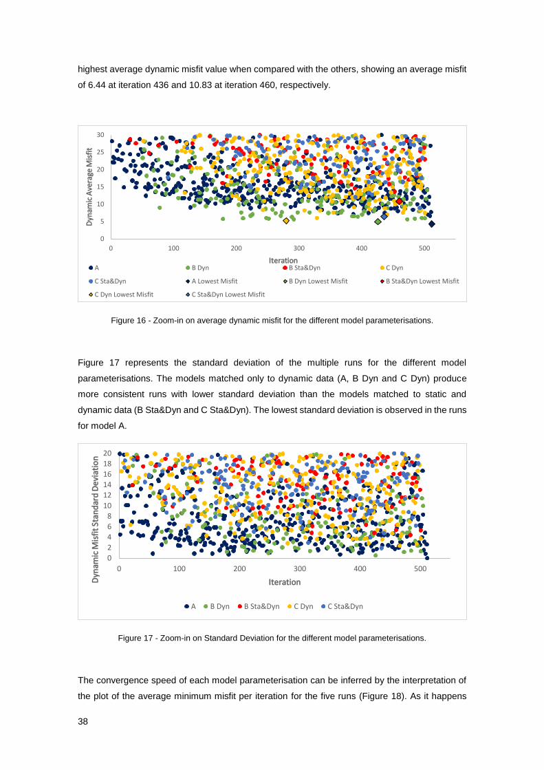
38
highest average dynamic misfit value when compared with the others, showing an average misfit
of 6.44 at iteration 436 and 10.83 at iteration 460, respectively.
Figure 16 - Zoom-in on average dynamic misfit for the different model parameterisations.
Figure 17 represents the standard deviation of the multiple runs for the different model
parameterisations. The models matched only to dynamic data (A, B Dyn and C Dyn) produce
more consistent runs with lower standard deviation than the models matched to static and
dynamic data (B Sta&Dyn and C Sta&Dyn). The lowest standard deviation is observed in the runs
for model A.
Figure 17 - Zoom-in on Standard Deviation for the different model parameterisations.
The convergence speed of each model parameterisation can be inferred by the interpretation of
the plot of the average minimum misfit per iteration for the five runs (Figure 18). As it happens
0
5
10
15
20
25
30
0 100 200 300 400 500
Dyn
amic
Ave
rage
Mis
fit
IterationA B Dyn B Sta&Dyn C Dyn
C Sta&Dyn A Lowest Misfit B Dyn Lowest Misfit B Sta&Dyn Lowest Misfit
C Dyn Lowest Misfit C Sta&Dyn Lowest Misfit
0
2
4
6
8
10
12
14
16
18
20
0 100 200 300 400 500
Dyn
amic
Mis
fit
Stan
dar
d D
evi
atio
n
Iteration
A B Dyn B Sta&Dyn C Dyn C Sta&Dyn
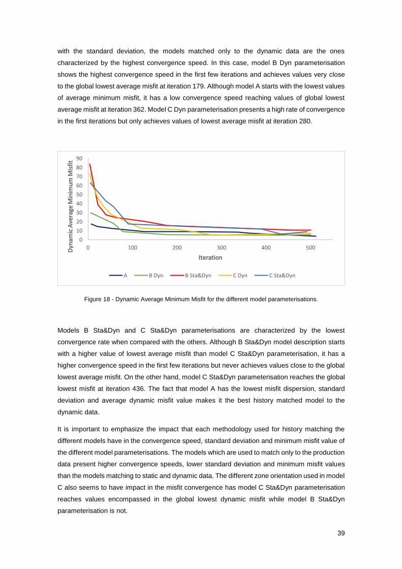
39
with the standard deviation, the models matched only to the dynamic data are the ones
characterized by the highest convergence speed. In this case, model B Dyn parameterisation
shows the highest convergence speed in the first few iterations and achieves values very close
to the global lowest average misfit at iteration 179. Although model A starts with the lowest values
of average minimum misfit, it has a low convergence speed reaching values of global lowest
average misfit at iteration 362. Model C Dyn parameterisation presents a high rate of convergence
in the first iterations but only achieves values of lowest average misfit at iteration 280.
Figure 18 - Dynamic Average Minimum Misfit for the different model parameterisations.
Models B Sta&Dyn and C Sta&Dyn parameterisations are characterized by the lowest
convergence rate when compared with the others. Although B Sta&Dyn model description starts
with a higher value of lowest average misfit than model C Sta&Dyn parameterisation, it has a
higher convergence speed in the first few iterations but never achieves values close to the global
lowest average misfit. On the other hand, model C Sta&Dyn parameterisation reaches the global
lowest misfit at iteration 436. The fact that model A has the lowest misfit dispersion, standard
deviation and average dynamic misfit value makes it the best history matched model to the
dynamic data.
It is important to emphasize the impact that each methodology used for history matching the
different models have in the convergence speed, standard deviation and minimum misfit value of
the different model parameterisations. The models which are used to match only to the production
data present higher convergence speeds, lower standard deviation and minimum misfit values
than the models matching to static and dynamic data. The different zone orientation used in model
C also seems to have impact in the misfit convergence has model C Sta&Dyn parameterisation
reaches values encompassed in the global lowest dynamic misfit while model B Sta&Dyn
parameterisation is not.
0
10
20
30
40
50
60
70
80
90
0 100 200 300 400 500Dyn
amic
Ave
rage
Min
imu
m M
isfi
t
Iteration
A B Dyn B Sta&Dyn C Dyn C Sta&Dyn
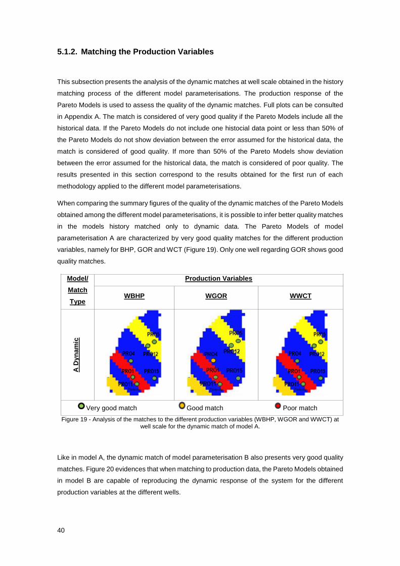
40
5.1.2. Matching the Production Variables
This subsection presents the analysis of the dynamic matches at well scale obtained in the history
matching process of the different model parameterisations. The production response of the
Pareto Models is used to assess the quality of the dynamic matches. Full plots can be consulted
in Appendix A. The match is considered of very good quality if the Pareto Models include all the
historical data. If the Pareto Models do not include one histocial data point or less than 50% of
the Pareto Models do not show deviation between the error assumed for the historical data, the
match is considered of good quality. If more than 50% of the Pareto Models show deviation
between the error assumed for the historical data, the match is considered of poor quality. The
results presented in this section correspond to the results obtained for the first run of each
methodology applied to the different model parameterisations.
When comparing the summary figures of the quality of the dynamic matches of the Pareto Models
obtained among the different model parameterisations, it is possible to infer better quality matches
in the models history matched only to dynamic data. The Pareto Models of model
parameterisation A are characterized by very good quality matches for the different production
variables, namely for BHP, GOR and WCT (Figure 19). Only one well regarding GOR shows good
quality matches.
Model/
Match
Type
Production Variables
WBHP WGOR WWCT
A D
yn
am
ic
Very good match Good match Poor match
Figure 19 - Analysis of the matches to the different production variables (WBHP, WGOR and WWCT) at well scale for the dynamic match of model A.
Like in model A, the dynamic match of model parameterisation B also presents very good quality
matches. Figure 20 evidences that when matching to production data, the Pareto Models obtained
in model B are capable of reproducing the dynamic response of the system for the different
production variables at the different wells.

41
The same does not happen with the static and dynamic match of model parameterisation B.
Regarding Borehole Pressure there is no well showing very good quality matches. For this
production variable three wells achieved good matches while the others present poor matches.
The Gas-Oil Ratio was the variable better matched in this model as it demonstrates five wells with
very good quality matches and one with good responses. Like Gas-Oil Ratio, the matches to
Water Cut are also of very good quality as only two wells show good matches and other presents
matches of poor quality.
Model/
Match
Type
Production Variables
WBHP WGOR WWCT
B S
tati
c&
Dyn
am
ic
B D
yn
am
ic
Very good match Good match Poor match
Figure 20 - Analysis of the matches to the different production variables (WBHP, WGOR and WWCT) at well scale for the dynamic and the static and dynamic matches of model B.
The overall quality of the matches in C Dyn model description for the production data is very good
(Figure 21). All wells have the ability to reproduce the historical dynamic response regarding the
different production variables matched.
Looking to the static and dynamic match of model parameterisation C, it is also possible to infer
overall good quality matches (Figure 21). Borehole Pressure appears with very good quality
matches at one well, good matches at four wells and only one well is characterized by poor quality
matches. Gas-Oil Ratio shows three wells with good matches having the rest three wells very
good quality matches. Water Cut is presented with a similar response to the truth regarding the
six wells.
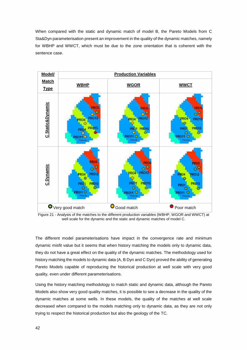
42
When compared with the static and dynamic match of model B, the Pareto Models from C
Sta&Dyn parameterisation present an improvement in the quality of the dynamic matches, namely
for WBHP and WWCT, which must be due to the zone orientation that is coherent with the
sentence case.
Model/
Match
Type
Production Variables
WBHP WGOR WWCT
C S
tati
c&
Dyn
am
ic
C D
yn
am
ic
Very good match Good match Poor match
Figure 21 - Analysis of the matches to the different production variables (WBHP, WGOR and WWCT) at well scale for the dynamic and the static and dynamic matches of model C.
The different model parameterisations have impact in the convergence rate and minimum
dynamic misfit value but it seems that when history matching the models only to dynamic data,
they do not have a great effect on the quality of the dynamic matches. The methodology used for
history matching the models to dynamic data (A, B Dyn and C Dyn) proved the ability of generating
Pareto Models capable of reproducing the historical production at well scale with very good
quality, even under different parameterisations.
Using the history matching methodology to match static and dynamic data, although the Pareto
Models also show very good quality matches, it is possible to see a decrease in the quality of the
dynamic matches at some wells. In these models, the quality of the matches at well scale
decreased when compared to the models matching only to dynamic data, as they are not only
trying to respect the historical production but also the geology of the TC.
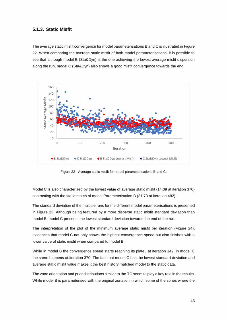
43
5.1.3. Static Misfit
The average static misfit convergence for model parameterisations B and C is illustrated in Figure
22. When comparing the average static misfit of both model parameterisations, it is possible to
see that although model B (Sta&Dyn) is the one achieving the lowest average misfit dispersion
along the run, model C (Sta&Dyn) also shows a good misfit convergence towards the end.
Figure 22 - Average static misfit for model parameterisations B and C.
Model C is also characterized by the lowest value of average static misfit (14.09 at iteration 370)
contrasting with the static match of model Parameterisation B (31.78 at iteration 482).
The standard deviation of the multiple runs for the different model parameterisations is presented
in Figure 23. Although being featured by a more disperse static misfit standard deviation than
model B, model C presents the lowest standard deviation towards the end of the run.
The interpretation of the plot of the minimum average static misfit per iteration (Figure 24),
evidences that model C not only shows the highest convergence speed but also finishes with a
lower value of static misfit when compared to model B.
While in model B the convergence speed starts reaching its plateu at iteration 142, in model C
the same happens at iteration 370. The fact that model C has the lowest standard deviation and
average static misfit value makes it the best history matched model to the static data.
The zone orientation and prior distributions similar to the TC seem to play a key role in the results.
While model B is parameterised with the original zonation in which some of the zones where the
0
20
40
60
80
100
120
140
160
0 100 200 300 400 500
Stat
ic A
vera
ge M
isfi
t
Iteration
B Sta&Dyn C Sta&Dyn B Sta&Dyn Lowest Misfit C Sta&Dyn Lowest Misfit

44
wells are placed are not geologically coherent with the reservoir, the zone orientation of model C
is consistent with the geology of the TC.
Figure 23 - Zoom-in on Standard Deviation for model parameterisations B and C.
The geological consistency of the new zone orientation as well as the application of the truth case
distributions have impact in the increase of the speed convergence, lower average standard
deviation towards the end and lowest average misfit value.
Figure 24 - Static Average Minimum Misfit for model parameterisations B and C.
0
5
10
15
20
25
30
35
40
45
50
0 100 200 300 400 500
Stat
ic M
isfi
t St
and
ard
De
viat
ion
Iteration
B Sta&Dyn C Sta&Dyn
0
10
20
30
40
50
60
70
80
0 100 200 300 400 500
Stat
ic A
vera
ge M
inim
um
Mis
fit
Iteration
B Sta&Dyn C Sta&Dyn
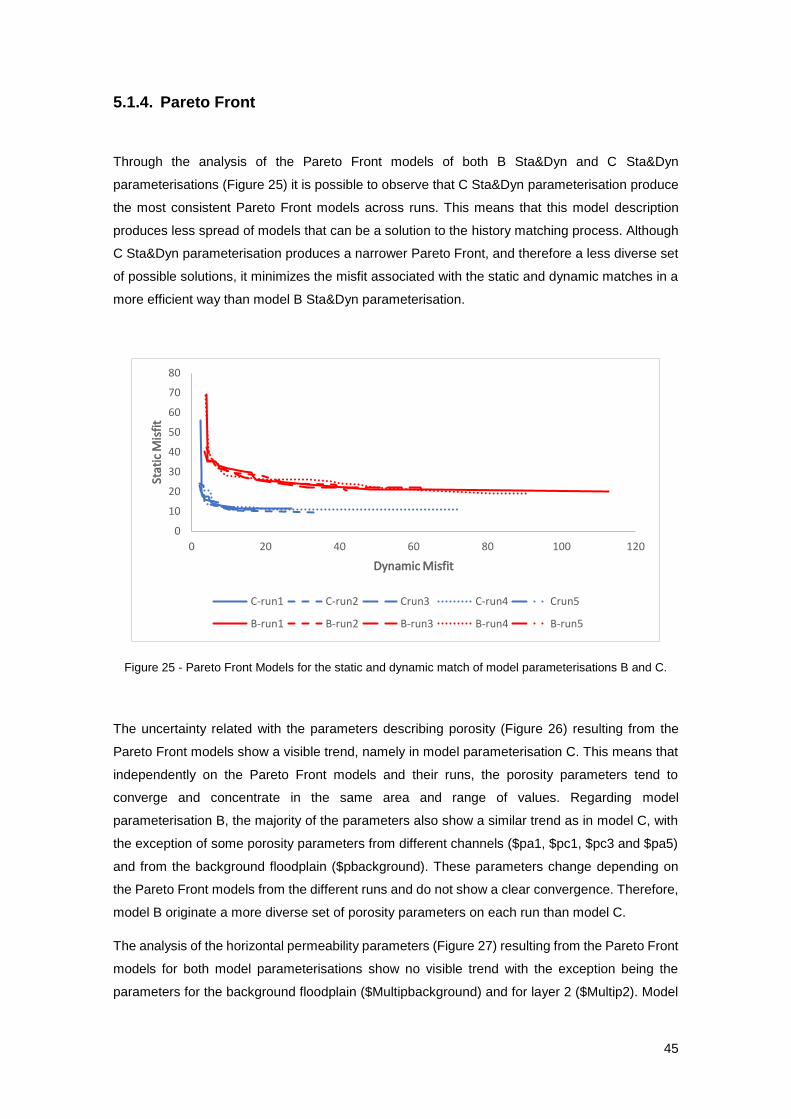
45
5.1.4. Pareto Front
Through the analysis of the Pareto Front models of both B Sta&Dyn and C Sta&Dyn
parameterisations (Figure 25) it is possible to observe that C Sta&Dyn parameterisation produce
the most consistent Pareto Front models across runs. This means that this model description
produces less spread of models that can be a solution to the history matching process. Although
C Sta&Dyn parameterisation produces a narrower Pareto Front, and therefore a less diverse set
of possible solutions, it minimizes the misfit associated with the static and dynamic matches in a
more efficient way than model B Sta&Dyn parameterisation.
Figure 25 - Pareto Front Models for the static and dynamic match of model parameterisations B and C.
The uncertainty related with the parameters describing porosity (Figure 26) resulting from the
Pareto Front models show a visible trend, namely in model parameterisation C. This means that
independently on the Pareto Front models and their runs, the porosity parameters tend to
converge and concentrate in the same area and range of values. Regarding model
parameterisation B, the majority of the parameters also show a similar trend as in model C, with
the exception of some porosity parameters from different channels ($pa1, $pc1, $pc3 and $pa5)
and from the background floodplain ($pbackground). These parameters change depending on
the Pareto Front models from the different runs and do not show a clear convergence. Therefore,
model B originate a more diverse set of porosity parameters on each run than model C.
The analysis of the horizontal permeability parameters (Figure 27) resulting from the Pareto Front
models for both model parameterisations show no visible trend with the exception being the
parameters for the background floodplain ($Multipbackground) and for layer 2 ($Multip2). Model
0
10
20
30
40
50
60
70
80
0 20 40 60 80 100 120
Stat
ic M
isfi
t
Dynamic Misfit
C-run1 C-run2 Crun3 C-run4 Crun5
B-run1 B-run2 B-run3 B-run4 B-run5

46
B also presents some horizontal permeability parameters from different channels ($Multipa1,
$Multipb1) characterized by convergence as they concentrate on the lower half of the range.
Figure 26 - Porosity of the Pareto Models obtained in the static and dynamic match of model
parameterisations B and C vs Static Misfit.
Regarding the uncertain porosity parameters plotted versus the dynamic misfit (Figure 28) for
both model parameterisations, there is no visible trend as the parameters change depending on
the Pareto Front models and their runs. A clear parameter convergence does not occur with the
exceptions being two channel parameters from layer 5 ($pb5 and $pc5), layer 2 ($p2) and layer
0
0,1
0,2
0,3
0,4
0 20 40 60 80
$p
a1
Static Misfit
0
0,1
0,2
0,3
0,4
0 50 100$
pb
1Static Misfit
0
0,1
0,2
0,3
0,4
0 20 40 60 80
$p
c1
Static Misfit
0
0,1
0,2
0,3
0,4
0 50 100
$p
a3
Static Misfit
0
0,1
0,2
0,3
0,4
0 50 100
$p
b3
Static Misfit
0
0,1
0,2
0,3
0,4
0 50 100
$p
c3
Static Misfit
0
0,1
0,2
0,3
0,4
0 20 40 60 80
$p
a5
Static Misfit
0
0,1
0,2
0,3
0,4
0 20 40 60 80
$p
b5
Static Misfit
0
0,1
0,2
0,3
0,4
0 50 100
$p
c5
Static Misfit
0
0,1
0,2
0,3
0,4
0 50 100
$b
ackg
rou
nd
Static Misfit
0
0,05
0,1
0,15
0 20 40 60 80
$p
2
Static Misfit
0
0,05
0,1
0,15
0,2
0,25
0 50 100
$p
4
Static Misfit
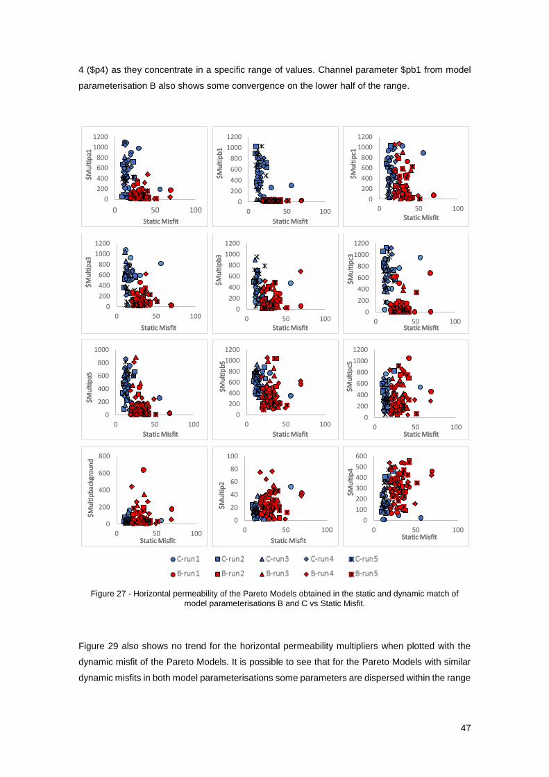
47
4 ($p4) as they concentrate in a specific range of values. Channel parameter $pb1 from model
parameterisation B also shows some convergence on the lower half of the range.
Figure 27 - Horizontal permeability of the Pareto Models obtained in the static and dynamic match of
model parameterisations B and C vs Static Misfit.
Figure 29 also shows no trend for the horizontal permeability multipliers when plotted with the
dynamic misfit of the Pareto Models. It is possible to see that for the Pareto Models with similar
dynamic misfits in both model parameterisations some parameters are dispersed within the range
0
200
400
600
800
1000
1200
0 50 100
$M
ult
ipa1
Static Misfit
0
200
400
600
800
1000
1200
0 50 100$
Mu
ltip
b1
Static Misfit
0
200
400
600
800
1000
1200
0 50 100
$M
ult
ipc1
Static Misfit
0
200
400
600
800
1000
1200
0 50 100
$M
ult
ipa3
Static Misfit
0
200
400
600
800
1000
1200
0 50 100
$M
ult
ipb
3
Static Misfit
0
200
400
600
800
1000
1200
0 50 100
$M
ult
ipc3
Static Misfit
0
200
400
600
800
1000
0 50 100
$M
ult
ipa5
Static Misfit
0
200
400
600
800
1000
1200
0 50 100
$M
ult
ipb
5
Static Misfit
0
200
400
600
800
1000
1200
0 50 100
$M
ult
ipc5
Static Misfit
0
200
400
600
800
0 50 100
$M
ult
ipb
ackg
rou
nd
Static Misfit
0
20
40
60
80
100
0 50 100
$M
ult
ip2
Static Misfit
0
100
200
300
400
500
600
0 50 100
$M
ult
ip4
Static Misfit

48
they can vary. Moreover, there are also parameters concentrated in the same range of values
corresponding to different misfits of Pareto Models, especially for model B parameterisation.
Figure 28 - Porosity of the Pareto Models obtained in the static and dynamic match of model
parameterisations B and C vs Dynamic Misfit.
Under the different model parameterisations, it seems that the different parameters dispersed
within several range of values can reproduce the dynamic response of the truth case, leading to
a low value of dynamic misfit in the Pareto Models. On the other hand, the value of the static misfit
only decreases when the parameters of the Pareto Models converge to a specific range of values.
0
0,1
0,2
0,3
0,4
0 50 100 150
$p
a1
Dynamic Misfit
0
0,1
0,2
0,3
0,4
0 50 100 150$
pb
1Dynamic Misfit
0
0,1
0,2
0,3
0,4
0 100 200
$p
c1
Dynamic Misfit
0
0,1
0,2
0,3
0,4
0 100 200
$p
a3
Dynamic Misfit
0
0,1
0,2
0,3
0,4
0 100 200
$p
b3
Dynamic Misfit
0
0,1
0,2
0,3
0,4
0 100 200
$p
c3
Dynamic Misfit
0
0,1
0,2
0,3
0,4
0 100 200
$p
a5
Dynamic Misfit
0
0,1
0,2
0,3
0,4
0 100 200
$p
b5
Dynamic Misfit
0
0,1
0,2
0,3
0,4
0 100 200
$p
c5
Dynamic Misfit
0
0,1
0,2
0,3
0,4
0 100 200
$b
ackg
rou
nd
Dynamic Misfit
0
0,05
0,1
0,15
0 100 200
$p
2
Dynamic Misfit
0
0,05
0,1
0,15
0,2
0,25
0 100 200
$p
4
Dynamic Misfit
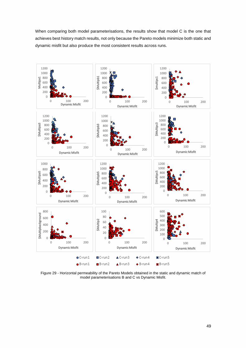
49
When comparing both model parameterisations, the results show that model C is the one that
achieves best history match results, not only because the Pareto models minimize both static and
dynamic misfit but also produce the most consistent results across runs.
Figure 29 - Horizontal permeability of the Pareto Models obtained in the static and dynamic match of model parameterisations B and C vs Dynamic Misfit.
0
200
400
600
800
1000
1200
0 100 200
Mu
ltip
a1
Dynamic Misfit
0
200
400
600
800
1000
1200
0 100 200$
Mu
ltip
b1
Dynamic Misfit
0
200
400
600
800
1000
1200
0 100 200
$m
ult
ipc1
Dynamic Misfit
0
200
400
600
800
1000
1200
0 100 200
$M
ult
ipa3
Dynamic Misfit
0
200
400
600
800
1000
1200
0 100 200
$M
ult
ipb
3
Dynamic Misfit
0
200
400
600
800
1000
1200
0 100 200
$M
ult
ipc3
Dynamic Misfit
0
200
400
600
800
1000
0 100 200
$M
ult
ipa5
Dynamic Misfit
0
200
400
600
800
1000
1200
0 100 200
$M
ult
ipb
5
Dynamic Misfit
0
200
400
600
800
1000
1200
0 100 200
$M
ult
ipc5
Dynamic Misfit
0
200
400
600
800
0 100 200
$M
ult
ipb
ackg
rou
nd
Dynamic Misfit
0
20
40
60
80
100
0 100 200
$M
ult
ip2
Dynamic Misfit
0
100
200
300
400
500
600
0 100 200
$M
ult
ip4
Dynamic Misfit

50
5.2. Geologial Consistency
The geological consistency of the different model parameterisations is inferred by evaluating the
quality of the static matches (porosity, horizontal permeability and vertical permeability) at well
scale by facies type from the Pareto Models. As models A, B dyn and C dyn parameterisations
were only history matched to dynamic data, for terms of comparison their static matches were
computed after running the history matching procedure.
The porosity versus horizontal permeability (Phi/PermX) and horizontal permeability versus
vertical permeability (PermX/PermZ) joint distributions of the Pareto Models from the different
model parameterisations are plotted. These joint distributions are plotted together with the same
joint distributions from the TC in order to evaluate the overall model distributions and validate the
geological consistency. The results presented in this section correspond to the results obtained
for the first run of each methodology applied to the different model parameterisations.
5.2.1. Static Matches
Through the analysis of the Figures below it is possible to interpret that there are some differences
in the quality of the static matches at well scale by facies type among the different model
parameterisations.
• Fluvial Channel Fills
Model parameterisation A is the one characterized by the poorest quality matches for the three
petrophysical properties (Figure 30).
Model A
Wells:
1 - PRO1 Layer 5; 2 – PRO4 Layer 1; 3 – PRO4 Layer 5; 4 – PRO5 Layer 1; 5 – PRO5 Layer 3; 6 – PRO11 Layer 3;
7 – PRO11 Layer 5; 8 – PRO12 Layer 5; 9 – PRO15 Layer1; 10 – PRO15 Layer 3; 11 – PRO15 Layer 5.
Figure 30 - Static (porosity, horizontal permeability and vertical permeability) matches at well scale of model A for fluvial channel fills facies type.
0
0,1
0,2
0,3
0,4
0 1 2 3 4 5 6 7 8 9 1011
Ph
i (fr
acti
on
)
Wells
0
1000
2000
3000
4000
5000
6000
0 1 2 3 4 5 6 7 8 9 1011
Pe
rmX
(mD
)
Wells
0
100
200
300
400
500
600
0 1 2 3 4 5 6 7 8 9 1011
Pe
rmZ
(mD
)
Wells
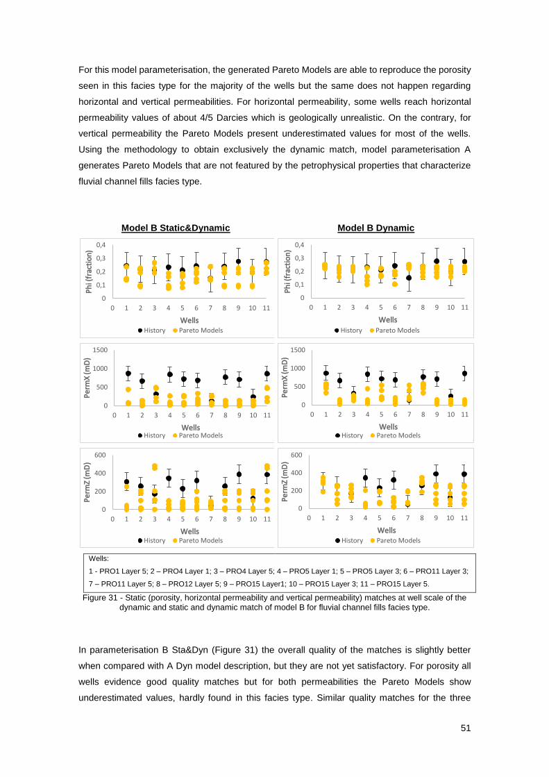
51
For this model parameterisation, the generated Pareto Models are able to reproduce the porosity
seen in this facies type for the majority of the wells but the same does not happen regarding
horizontal and vertical permeabilities. For horizontal permeability, some wells reach horizontal
permeability values of about 4/5 Darcies which is geologically unrealistic. On the contrary, for
vertical permeability the Pareto Models present underestimated values for most of the wells.
Using the methodology to obtain exclusively the dynamic match, model parameterisation A
generates Pareto Models that are not featured by the petrophysical properties that characterize
fluvial channel fills facies type.
Model B Static&Dynamic Model B Dynamic
Wells:
1 - PRO1 Layer 5; 2 – PRO4 Layer 1; 3 – PRO4 Layer 5; 4 – PRO5 Layer 1; 5 – PRO5 Layer 3; 6 – PRO11 Layer 3;
7 – PRO11 Layer 5; 8 – PRO12 Layer 5; 9 – PRO15 Layer1; 10 – PRO15 Layer 3; 11 – PRO15 Layer 5.
Figure 31 - Static (porosity, horizontal permeability and vertical permeability) matches at well scale of the dynamic and static and dynamic match of model B for fluvial channel fills facies type.
In parameterisation B Sta&Dyn (Figure 31) the overall quality of the matches is slightly better
when compared with A Dyn model description, but they are not yet satisfactory. For porosity all
wells evidence good quality matches but for both permeabilities the Pareto Models show
underestimated values, hardly found in this facies type. Similar quality matches for the three
0
0,1
0,2
0,3
0,4
0 1 2 3 4 5 6 7 8 9 10 11
Ph
i (fr
acti
on
)
WellsHistory Pareto Models
0
0,1
0,2
0,3
0,4
0 1 2 3 4 5 6 7 8 9 10 11
Ph
i (fr
acti
on
)
WellsHistory Pareto Models
0
500
1000
1500
0 1 2 3 4 5 6 7 8 9 10 11
Pe
rmX
(mD
)
WellsHistory Pareto Models
0
500
1000
1500
0 1 2 3 4 5 6 7 8 9 10 11
Pe
rmX
(mD
)
WellsHistory Pareto Models
0
200
400
600
0 1 2 3 4 5 6 7 8 9 10 11
Pe
rmZ
(mD
)
WellsHistory Pareto Models
0
200
400
600
0 1 2 3 4 5 6 7 8 9 10 11
Pe
rmZ
(mD
)
WellsHistory Pareto Models
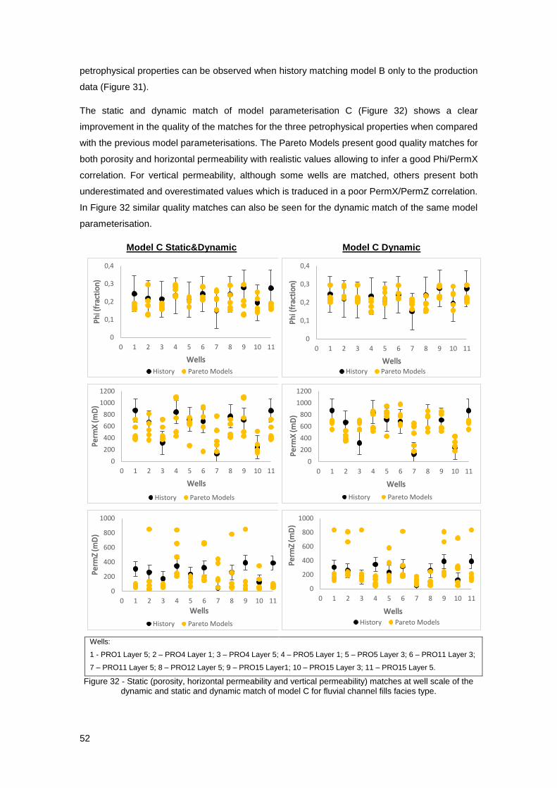
52
petrophysical properties can be observed when history matching model B only to the production
data (Figure 31).
The static and dynamic match of model parameterisation C (Figure 32) shows a clear
improvement in the quality of the matches for the three petrophysical properties when compared
with the previous model parameterisations. The Pareto Models present good quality matches for
both porosity and horizontal permeability with realistic values allowing to infer a good Phi/PermX
correlation. For vertical permeability, although some wells are matched, others present both
underestimated and overestimated values which is traduced in a poor PermX/PermZ correlation.
In Figure 32 similar quality matches can also be seen for the dynamic match of the same model
parameterisation.
Model C Static&Dynamic Model C Dynamic
Wells:
1 - PRO1 Layer 5; 2 – PRO4 Layer 1; 3 – PRO4 Layer 5; 4 – PRO5 Layer 1; 5 – PRO5 Layer 3; 6 – PRO11 Layer 3;
7 – PRO11 Layer 5; 8 – PRO12 Layer 5; 9 – PRO15 Layer1; 10 – PRO15 Layer 3; 11 – PRO15 Layer 5.
Figure 32 - Static (porosity, horizontal permeability and vertical permeability) matches at well scale of the dynamic and static and dynamic match of model C for fluvial channel fills facies type.
0
0,1
0,2
0,3
0,4
0 1 2 3 4 5 6 7 8 9 10 11
Ph
i (fr
acti
on
)
Wells
History Pareto Models
0
0,1
0,2
0,3
0,4
0 1 2 3 4 5 6 7 8 9 10 11
Ph
i (fr
acti
on
)
WellsHistory Pareto Models
0
200
400
600
800
1000
1200
0 1 2 3 4 5 6 7 8 9 10 11
Pe
rmX
(mD
)
Wells
History Pareto Models
0
200
400
600
800
1000
1200
0 1 2 3 4 5 6 7 8 9 10 11
Pe
rmX
(mD
)
Wells
History Pareto Models
0
200
400
600
800
1000
0 1 2 3 4 5 6 7 8 9 10 11
Pe
rmZ
(mD
)
Wells
History Pareto Models
0
200
400
600
800
1000
0 1 2 3 4 5 6 7 8 9 10 11
Pe
rmZ
(mD
)
Wells
History Pareto Models
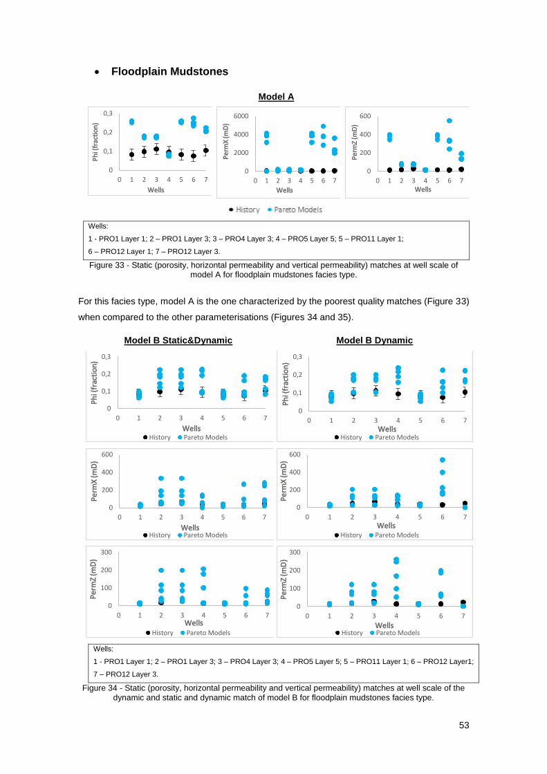
53
• Floodplain Mudstones
Model A
Wells:
1 - PRO1 Layer 1; 2 – PRO1 Layer 3; 3 – PRO4 Layer 3; 4 – PRO5 Layer 5; 5 – PRO11 Layer 1;
6 – PRO12 Layer 1; 7 – PRO12 Layer 3.
Figure 33 - Static (porosity, horizontal permeability and vertical permeability) matches at well scale of model A for floodplain mudstones facies type.
For this facies type, model A is the one characterized by the poorest quality matches (Figure 33)
when compared to the other parameterisations (Figures 34 and 35).
Model B Static&Dynamic Model B Dynamic
Wells:
1 - PRO1 Layer 1; 2 – PRO1 Layer 3; 3 – PRO4 Layer 3; 4 – PRO5 Layer 5; 5 – PRO11 Layer 1; 6 – PRO12 Layer1;
7 – PRO12 Layer 3.
Figure 34 - Static (porosity, horizontal permeability and vertical permeability) matches at well scale of the dynamic and static and dynamic match of model B for floodplain mudstones facies type.
0
0,1
0,2
0,3
0 1 2 3 4 5 6 7
Ph
i (fr
acti
on
)
Wells
0
2000
4000
6000
0 1 2 3 4 5 6 7
Pe
rmX
(mD
)
Wells
0
200
400
600
0 1 2 3 4 5 6 7
Pe
rmZ
(mD
)
Wells
0
0,1
0,2
0,3
0 1 2 3 4 5 6 7
Ph
i (fr
acti
on
)
WellsHistory Pareto Models
0
0,1
0,2
0,3
0 1 2 3 4 5 6 7
Ph
i (fr
acti
on
)
WellsHistory Pareto Models
0
200
400
600
0 1 2 3 4 5 6 7
Pe
rmX
(mD
)
WellsHistory Pareto Models
0
200
400
600
0 1 2 3 4 5 6 7
Pe
rmX
(mD
)
WellsHistory Pareto Models
0
100
200
300
0 1 2 3 4 5 6 7
Pe
rmZ
(mD
)
WellsHistory Pareto Models
0
100
200
300
0 1 2 3 4 5 6 7
Pe
rmZ
(mD
)
WellsHistory Pareto Models
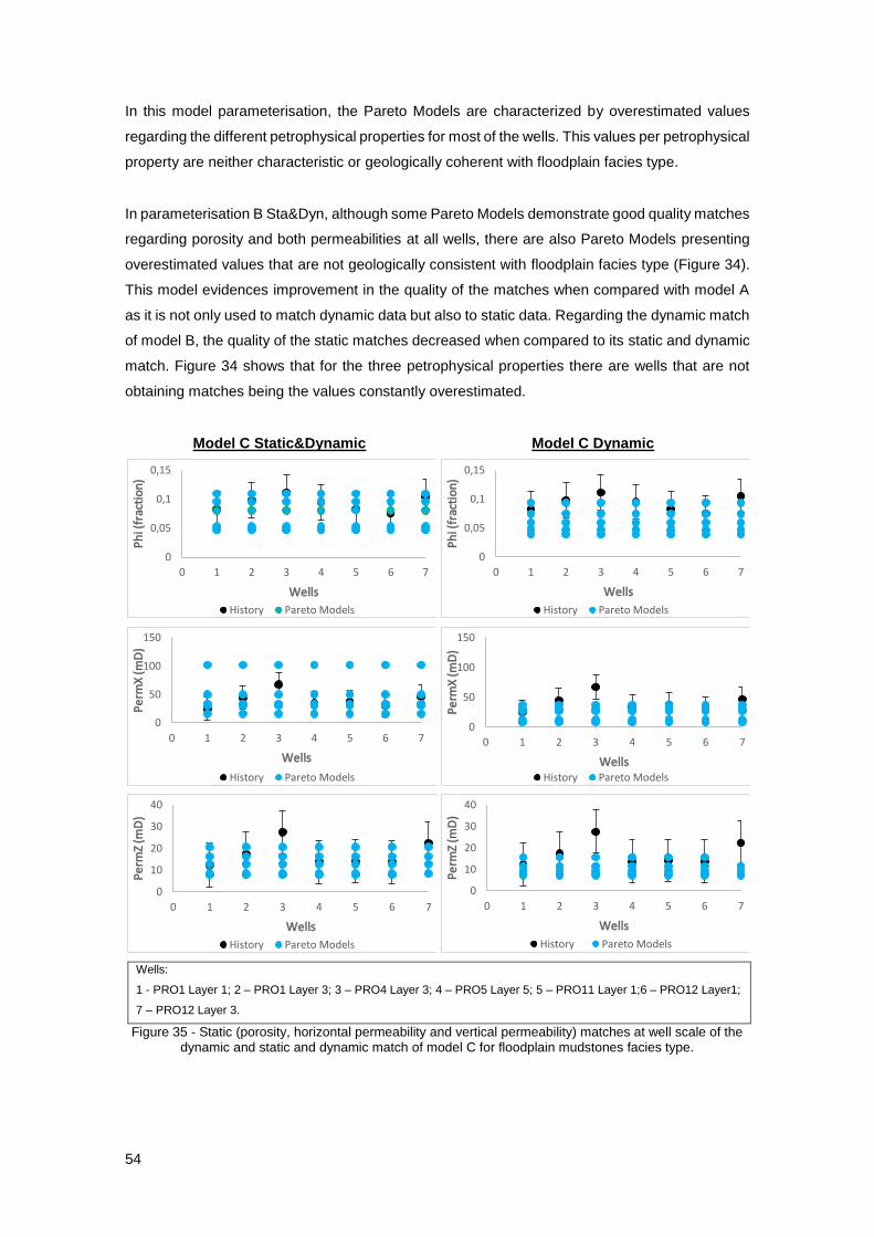
54
In this model parameterisation, the Pareto Models are characterized by overestimated values
regarding the different petrophysical properties for most of the wells. This values per petrophysical
property are neither characteristic or geologically coherent with floodplain facies type.
In parameterisation B Sta&Dyn, although some Pareto Models demonstrate good quality matches
regarding porosity and both permeabilities at all wells, there are also Pareto Models presenting
overestimated values that are not geologically consistent with floodplain facies type (Figure 34).
This model evidences improvement in the quality of the matches when compared with model A
as it is not only used to match dynamic data but also to static data. Regarding the dynamic match
of model B, the quality of the static matches decreased when compared to its static and dynamic
match. Figure 34 shows that for the three petrophysical properties there are wells that are not
obtaining matches being the values constantly overestimated.
Model C Static&Dynamic Model C Dynamic
Wells:
1 - PRO1 Layer 1; 2 – PRO1 Layer 3; 3 – PRO4 Layer 3; 4 – PRO5 Layer 5; 5 – PRO11 Layer 1;6 – PRO12 Layer1;
7 – PRO12 Layer 3.
Figure 35 - Static (porosity, horizontal permeability and vertical permeability) matches at well scale of the dynamic and static and dynamic match of model C for floodplain mudstones facies type.
0
0,05
0,1
0,15
0 1 2 3 4 5 6 7
Ph
i (fr
acti
on
)
Wells
History Pareto Models
0
0,05
0,1
0,15
0 1 2 3 4 5 6 7
Ph
i (fr
acti
on
)
Wells
History Pareto Models
0
50
100
150
0 1 2 3 4 5 6 7
Pe
rmX
(mD
)
Wells
History Pareto Models
0
50
100
150
0 1 2 3 4 5 6 7
Pe
rmX
(mD
)
WellsHistory Pareto Models
0
10
20
30
40
0 1 2 3 4 5 6 7
Pe
rmZ
(mD
)
Wells
History Pareto Models
0
10
20
30
40
0 1 2 3 4 5 6 7
Pe
rmZ
(mD
)
Wells
History Pareto Models
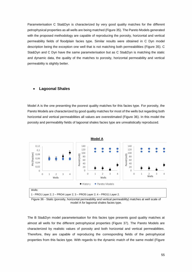
55
Parameterisation C Sta&Dyn is characterized by very good quality matches for the different
petrophysical properties as all wells are being matched (Figure 35). The Pareto Models generated
with the proposed methodology are capable of reproducing the porosity, horizontal and vertical
permeability fields of floodplain facies type. Similar results were obtained in C Dyn model
description being the exception one well that is not matching both permeabilities (Figure 35). C
Sta&Dyn and C Dyn have the same parameterisation but as C Sta&Dyn is matching the static
and dynamic data, the quality of the matches to porosity, horizontal permeability and vertical
permeability is slightly better.
• Lagoonal Shales
Model A is the one presenting the poorest quality matches for this facies type. For porosity, the
Pareto Models are characterized by good quality matches for most of the wells but regarding both
horizontal and vertical permeabilities all values are overestimated (Figure 36). In this model the
porosity and permeability fields of lagoonal shales facies type are unrealistically reproduced.
Model A
Wells:
1 - PRO1 Layer 2; 2 – PRO4 Layer 2; 3 – PRO5 Layer 2; 4 – PRO11 Layer 2.
Figure 36 - Static (porosity, horizontal permeability and vertical permeability) matches at well scale of
model A for lagoonal shales facies type.
The B Sta&Dyn model parameterisation for this facies type presents good quality matches at
almost all wells for the different petrophysical properties (Figure 37). The Pareto Models are
characterized by realistic values of porosity and both horizontal and vertical permeabilities.
Therefore, they are capable of reproducing the corresponding fields of the petrophysical
properties from this facies type. With regards to the dynamic match of the same model (Figure
0
0,02
0,04
0,06
0,08
0,1
0,12
0 1 2 3 4
Ph
i (fr
acti
on
)
Wells
0
20
40
60
80
100
120
140
0 1 2 3 4
Pe
rmX
(mD
)
Wells
0
20
40
60
80
100
120
140
0 1 2 3 4
Pe
rmX
(mD
)
Wells

56
37), besides the decrease in the quality of the matches at some wells for vertical permeability,
similar results can be seen to those obtained with the proposed methodology.
Model B Static&Dynamic Model B Dynamic
Wells:
1 - PRO1 Layer 2; 2 – PRO4 Layer 2; 3 – PRO5 Layer 2; 4 – PRO11 Layer 2.
Figure 37 - Static (porosity, horizontal permeability and vertical permeability) matches at well scale of the dynamic and static and dynamic match of model B for lagoonal shales facies type.
In C Sta&Dyn and C Dyn model descriptions (Figure 38) the quality of the matches is quite similar
for the three properties and improved when compared to the other model parameterisations. For
both methodologies, the obtained Pareto Models are characterized by realistic values of porosity,
horizontal and vertical permeabilities, being geologically consistent with lagoonal shales facies
type.
0
0,05
0,1
0,15
0 1 2 3 4
Ph
i (fr
acti
on
)
Wells
History Pareto Models
0
0,05
0,1
0,15
0 1 2 3 4
Ph
i (fr
acti
on
)
WellsHistory Pareto Models
0
10
20
30
40
50
0 1 2 3 4
Pe
rmX
(mD
)
WellsHistory Pareto Models
0
10
20
30
40
50
0 1 2 3 4
Pe
rmX
(mD
)
WellsHistory Pareto Models
0
5
10
15
20
0 1 2 3 4
Pe
rmZ
(mD
)
WellsHistory Pareto Models
0
5
10
15
20
0 1 2 3 4
Pe
rmZ
(mD
)
WellsHistory Pareto Models
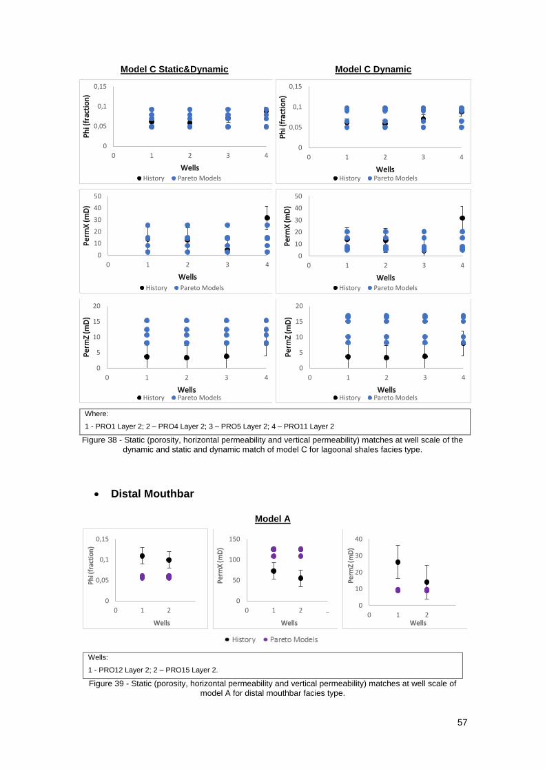
57
Model C Static&Dynamic Model C Dynamic
Where:
1 - PRO1 Layer 2; 2 – PRO4 Layer 2; 3 – PRO5 Layer 2; 4 – PRO11 Layer 2
Figure 38 - Static (porosity, horizontal permeability and vertical permeability) matches at well scale of the dynamic and static and dynamic match of model C for lagoonal shales facies type.
• Distal Mouthbar
Model A
Wells:
1 - PRO12 Layer 2; 2 – PRO15 Layer 2.
Figure 39 - Static (porosity, horizontal permeability and vertical permeability) matches at well scale of model A for distal mouthbar facies type.
0
0,05
0,1
0,15
0 1 2 3 4
Ph
i (fr
acti
on
)
WellsHistory Pareto Models
0
0,05
0,1
0,15
0 1 2 3 4
Ph
i (fr
acti
on
)
WellsHistory Pareto Models
0
10
20
30
40
50
0 1 2 3 4
Pe
rmX
(mD
)
Wells
History Pareto Models
0
10
20
30
40
50
0 1 2 3 4
Pe
rmX
(mD
)Wells
History Pareto Models
0
5
10
15
20
0 1 2 3 4
Pe
rmZ
(mD
)
WellsHistory Pareto Models
0
5
10
15
20
0 1 2 3 4
Pe
rmZ
(mD
)
WellsHistory Pareto Models
0
0,05
0,1
0,15
0 1 2 3
Ph
i (fr
acti
on
)
Wells
0
50
100
150
0 1 2 3
Pe
rmX
(mD
)
Wells
0
10
20
30
40
0 1 2 3
Pe
rmZ
(mD
)
Wells
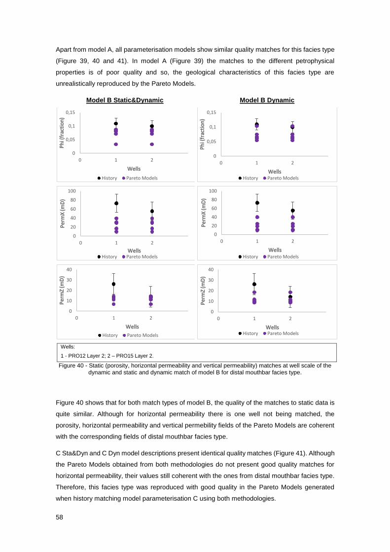
58
Apart from model A, all parameterisation models show similar quality matches for this facies type
(Figure 39, 40 and 41). In model A (Figure 39) the matches to the different petrophysical
properties is of poor quality and so, the geological characteristics of this facies type are
unrealistically reproduced by the Pareto Models.
Model B Static&Dynamic Model B Dynamic
Wells:
1 - PRO12 Layer 2; 2 – PRO15 Layer 2.
Figure 40 - Static (porosity, horizontal permeability and vertical permeability) matches at well scale of the dynamic and static and dynamic match of model B for distal mouthbar facies type.
Figure 40 shows that for both match types of model B, the quality of the matches to static data is
quite similar. Although for horizontal permeability there is one well not being matched, the
porosity, horizontal permeability and vertical permebility fields of the Pareto Models are coherent
with the corresponding fields of distal mouthbar facies type.
C Sta&Dyn and C Dyn model descriptions present identical quality matches (Figure 41). Although
the Pareto Models obtained from both methodologies do not present good quality matches for
horizontal permeability, their values still coherent with the ones from distal mouthbar facies type.
Therefore, this facies type was reproduced with good quality in the Pareto Models generated
when history matching model parameterisation C using both methodologies.
0
0,05
0,1
0,15
0 1 2 3
Ph
i (fr
acti
on
)
Wells
History Pareto Models
0
0,05
0,1
0,15
0 1 2 3
Ph
i (fr
acti
on
)
WellsHistory Pareto Models
0
20
40
60
80
100
0 1 2 3
Pe
rmX
(mD
)
WellsHistory Pareto Models
0
20
40
60
80
100
0 1 2 3
Pe
rmX
(mD
)
WellsHistory Pareto Models
0
10
20
30
40
0 1 2 3
Pe
rmZ
(mD
)
Wells
History Pareto Models
0
10
20
30
40
0 1 2 3
Pe
rmZ
(mD
)
WellsHistory Pareto Models
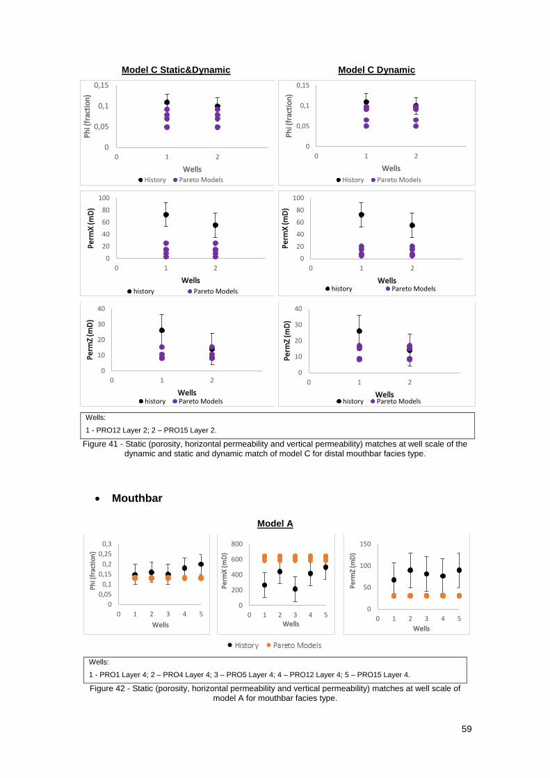
59
Model C Static&Dynamic Model C Dynamic
Wells:
1 - PRO12 Layer 2; 2 – PRO15 Layer 2.
Figure 41 - Static (porosity, horizontal permeability and vertical permeability) matches at well scale of the dynamic and static and dynamic match of model C for distal mouthbar facies type.
• Mouthbar
Model A
Wells:
1 - PRO1 Layer 4; 2 – PRO4 Layer 4; 3 – PRO5 Layer 4; 4 – PRO12 Layer 4; 5 – PRO15 Layer 4.
Figure 42 - Static (porosity, horizontal permeability and vertical permeability) matches at well scale of model A for mouthbar facies type.
0
0,05
0,1
0,15
0 1 2 3
Ph
i (fr
acti
on
)
WellsHistory Pareto Models
0
0,05
0,1
0,15
0 1 2 3
Ph
i (fr
acti
on
)
Wells
History Pareto Models
0
20
40
60
80
100
0 1 2 3
Pe
rmX
(mD
)
Wells
history Pareto Models
0
20
40
60
80
100
0 1 2 3
Pe
rmX
(mD
)Wells
history Pareto Models
0
10
20
30
40
0 1 2 3
Pe
rmZ
(mD
)
Wellshistory Pareto Models
0
10
20
30
40
0 1 2 3
Pe
rmZ
(mD
)
Wellshistory Pareto Models
0
0,05
0,1
0,15
0,2
0,25
0,3
0 1 2 3 4 5
Ph
i (fr
acti
on
)
Wells
0
200
400
600
800
0 1 2 3 4 5
Pe
rmX
(mD
)
Wells
0
50
100
150
0 1 2 3 4 5
Pe
rmZ
(mD
)
Wells
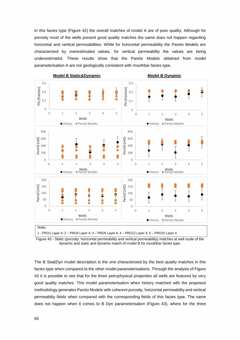
60
In this facies type (Figure 42) the overall matches of model A are of poor quality. Although for
porosity most of the wells present good quality matches the same does not happen regarding
horizontal and vertical permeabilities. While for horizontal permeability the Pareto Models are
characterized by overestimated values, for vertical permeability the values are being
underestimated. These results show that the Pareto Models obtained from model
parameterisation A are not geologically consistent with mouthbar facies type.
Model B Static&Dynamic Model B Dynamic
Wells:
1 - PRO1 Layer 4; 2 – PRO4 Layer 4; 3 – PRO5 Layer 4; 4 – PRO12 Layer 4; 5 – PRO15 Layer 4.
Figure 43 - Static (porosity, horizontal permeability and vertical permeability) matches at well scale of the
dynamic and static and dynamic match of model B for mouthbar facies type.
The B Sta&Dyn model description is the one characterized by the best quality matches in this
facies type when compared to the other model parameterisations. Through the analysis of Figure
43 it is possible to see that for the three petrophysical properties all wells are featured by very
good quality matches. This model parameterisation when history matched with the proposed
methodology generates Pareto Models with coherent porosity, horizontal permeability and vertical
permeabilty fields when compared with the corresponding fields of this facies type. The same
does not happen when it comes to B Dyn parameterisation (Figure 43), where for the three
0
0,1
0,2
0,3
0 1 2 3 4 5
Ph
i (fr
acti
on
)
Wells
History Pareto Models
0
0,1
0,2
0,3
0 1 2 3 4 5
Ph
i (fr
acti
on
)
WellsHistory Pareto Models
0
200
400
600
800
0 1 2 3 4 5
Pe
rmX
(mD
)
WellsHistory Pareto Models
0
200
400
600
800
0 1 2 3 4 5
Pe
rmX
(mD
)
WellsHistory Pareto Models
0
50
100
150
200
0 1 2 3 4 5
Pe
rmZ
(mD
)
WellsHistory Pareto Models
0
50
100
150
200
0 1 2 3 4 5
Pe
rmZ
(mD
)
WellsHistory Pareto Models

61
petrophysical properties there are some wells that are not being matched. Consequently, the
mouthbar facies type is not being realistically reproduced by the obtained Pareto Models.
In model description C Sta&Dyn the overall quality of the matches is good (Figure 44). For the
different petrophysical properties most of the wells are being matched and the correlations
between the petrophysical properties are geologically coherent with this facies type. The Pareto
Models generated are characterized by similar porosity, horizontal permeability and vertical
permeability fields as in mouthbar facies type. Model parameterisation C Dyn appears in this
facies type with the poorest quality matches among the different model parameterisations (Figure
44). The Pareto Models present overestimated values for most of the wells regarding the different
petrophysical properties. Therefore, there is an evident lack in geological consistency when
comparing their petrophysical property fields with the corresponding fields of mouthbar facies
type.
Model C Static&Dynamic Model C Dynamic
Wells:
1 - PRO1 Layer4; 2 – PRO4 Layer4; 3 – PRO5 Layer4; 4 – PRO11 Layer 4; 5 – PRO12 Layer 4; 6 – PRO15 Layer 4.
Figure 44 - Static (porosity, horizontal permeability and vertical permeability) matches at well scale of the dynamic and static and dynamic match of model C for mouthbar facies type.
0
0,1
0,2
0,3
0 1 2 3 4 5 6
Ph
i (fr
acti
on
)
Wells
history Pareto Models
0
0,1
0,2
0,3
0 1 2 3 4 5 6
Ph
i (fr
acti
on
)
Wells
history Pareto Models
0
200
400
600
800
0 1 2 3 4 5 6
Pe
rmX
(mD
)
Wells
history Pareto Models
0
200
400
600
800
0 1 2 3 4 5 6
Pe
rmX
(mD
)
Wells
history Pareto Models
0
50
100
150
200
0 1 2 3 4 5 6
Pe
rmZ
(mD
)
Wellshistory Pareto Models
0
50
100
150
200
0 2 4 6
Pe
rmZ
(mD
)
Wellshistory Pareto Models
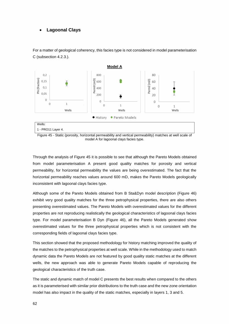
62
• Lagoonal Clays
For a matter of geological coherency, this facies type is not considered in model parameterisation
C (subsection 4.2.3.).
Model A
Wells:
1 - PRO11 Layer 4.
Figure 45 - Static (porosity, horizontal permeability and vertical permeability) matches at well scale of model A for lagoonal clays facies type.
Through the analysis of Figure 45 it is possible to see that although the Pareto Models obtained
from model parameterisation A present good quality matches for porosity and vertical
permeability, for horizontal permeability the values are being overestimated. The fact that the
horizontal permeability reaches values around 600 mD, makes the Pareto Models geologically
inconsistent with lagoonal clays facies type.
Although some of the Pareto Models obtained from B Sta&Dyn model description (Figure 46)
exhibit very good quality matches for the three petrophysical properties, there are also others
presenting overestimated values. The Pareto Models with overestimated values for the different
properties are not reproducing realistically the geological characteristics of lagoonal clays facies
type. For model parameterisation B Dyn (Figure 46), all the Pareto Models generated show
overestimated values for the three petrophysical properties which is not consistent with the
corresponding fields of lagoonal clays facies type.
This section showed that the proposed methodology for history matching improved the quality of
the matches to the petrophysical properties at well scale. While in the methodology used to match
dynamic data the Pareto Models are not featured by good quality static matches at the different
wells, the new approach was able to generate Pareto Models capable of reproducing the
geological characteristics of the truth case.
The static and dynamic match of model C presents the best results when compared to the others
as it is parameterised with similar prior distributions to the truth case and the new zone orientation
model has also impact in the quality of the static matches, especially in layers 1, 3 and 5.
0
0,05
0,1
0,15
0,2
0 1 2
Ph
i (fr
acti
on
)
Wells
0
200
400
600
800
0 1 2
Pe
rmX
(mD
)
Wells
0
20
40
60
80
0 1 2
Pe
rmZ
(mD
)
Wells

63
Model B Static&Dynamic Model B Dynamic
Wells:
1 - PRO11 Layer 4.
Figure 46 - Static (porosity, horizontal permeability and vertical permeability) matches at well scale of the dynamic and static and dynamic match of model B for lagoonal clays facies type.
5.2.2. Overall Distributions of the Pareto Models
The previous subsections encompassed the evaluation of the quality of the static matches at well
scale for the different model parameterisations regarding the three petrophysical properties. To
assess the geological consistency of the models, in this subsection the Phi/PermX and
PermX/PermZ bi-plots of the Pareto Models from each model parameterisation are plotted by
facies type, with the correspondent correlations from the TC. These correlations can be seen in
Figures 47 and 48.
Figure 47 illustrates the Phi/PermX and PermX/PermZ joint distributions of the Pareto Models for
Fluvial Channel Fills and Floodplain Mudstones facies type. For Fluvial Channel Fills it is possible
to observe that only model C for both methodologies (dynamic and static and dynamic matches)
respects the Phi/PermX joint distribution of the truth case. The parameters of the Pareto Models
from model C parameterisation with respect to this facies type, not only follow the same trend but
0
0,05
0,1
0,15
0,2
0,25
0 1 2
Ph
i (fr
acti
on
)
WellsHistory Pareto Models
0
0,05
0,1
0,15
0,2
0,25
0 1 2
Ph
i (fr
acti
on
)
WellsHistory Pareto Models
0
200
400
600
0 1 2
Pe
rmX
(mD
)
WellsHistory Pareto Models
0
200
400
600
0 1 2
Pe
rmX
(mD
)Wells
History Pareto Models
0
50
100
150
200
0 1 2
Pe
rmZ
(mD
)
WellsHistory Pareto Models
0
50
100
150
200
0 1 2
Pe
rmZ
(mD
)
WellsHistory Pareto Models

64
also have a similar dispersion as the TC. For both parameterisations B Dyn and B Sta&Dyn,
although there are some parameters that reproduce the joint distribution seen in the TC, others
are not following the same trend. Model A seems to be the one characterized by a completely
different joint distribution from the sentence case as there are parameters from the Pareto Models
not only underestimating but also overestimating this correlation. Regarding the PermX/PermZ
joint distribution of the Pareto Models for Fluvial Channel Fills, the same happens for the different
model parameterisations as with the Phi/PermX joint distribution.
For Floodplain Mudstones facies type, the Pareto Models of model A do not show the same
Phi/PermX joint distribution of the TC, as most of the parameters of the Pareto Models are
overestimating it. The majority of the Pareto Models of model parameterisations B Dyn and B
Sta&Dyn are also characterized by a different Phi/PermX joint distribution when compared to the
truth. Again, only model C in both methodologies is characterized by the same joint distribution
of the study case. When looking at the PermX/PermZ joint distribution for this facies type, only
model A is not featured by a similar joint distribution as in the TC.
Fluvial Channel Fills Floodplain Mudstones
Figure 47 - Comparison between the Phi/PermX and PermX/PermZ correlations of the Pareto Models of the different model parameterisations and the Truth Case for Fluvial Channel Fills and Foodplain facies
types.
Figure 48 shows the Phi/PermX and PermX/PermZ joint distributions of the Pareto Models plotted
with the same distributions of the sentence case for layers 2 and 4. Although both layers are
featured by different facies types, they are plotted as single layers as there are only one parameter
for porosity and another for horizontal permeability multiplier matching each layer.
0
0,5
1
1,5
2
2,5
3
3,5
4
0 0,1 0,2 0,3 0,4
log
Pe
rmX
Phi
0
0,5
1
1,5
2
2,5
3
3,5
4
0 0,1 0,2 0,3
log
Pe
rmX
Phi
0
0,5
1
1,5
2
2,5
3
3,5
0 1 2 3 4
log
Pe
rmZ
log PermX
0
0,5
1
1,5
2
2,5
3
0 1 2 3 4
log
Pe
rmZ
log PermX
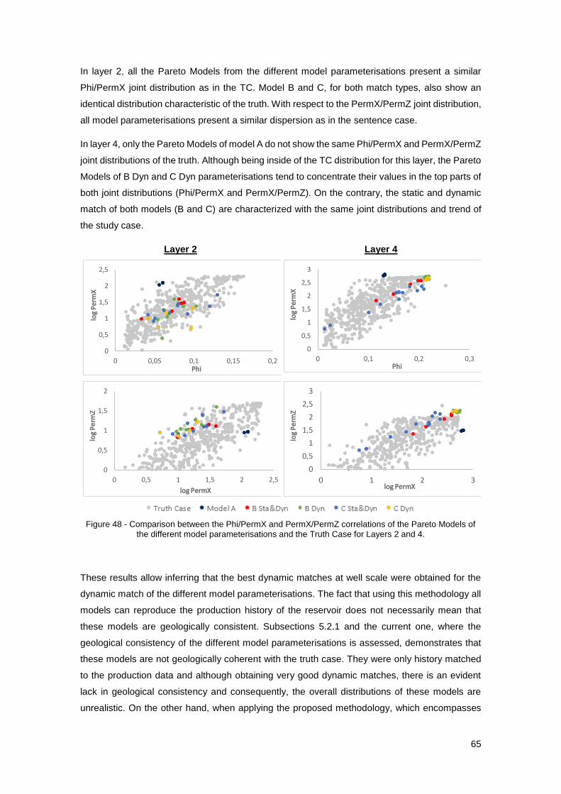
65
In layer 2, all the Pareto Models from the different model parameterisations present a similar
Phi/PermX joint distribution as in the TC. Model B and C, for both match types, also show an
identical distribution characteristic of the truth. With respect to the PermX/PermZ joint distribution,
all model parameterisations present a similar dispersion as in the sentence case.
In layer 4, only the Pareto Models of model A do not show the same Phi/PermX and PermX/PermZ
joint distributions of the truth. Although being inside of the TC distribution for this layer, the Pareto
Models of B Dyn and C Dyn parameterisations tend to concentrate their values in the top parts of
both joint distributions (Phi/PermX and PermX/PermZ). On the contrary, the static and dynamic
match of both models (B and C) are characterized with the same joint distributions and trend of
the study case.
Layer 2 Layer 4
Figure 48 - Comparison between the Phi/PermX and PermX/PermZ correlations of the Pareto Models of
the different model parameterisations and the Truth Case for Layers 2 and 4.
These results allow inferring that the best dynamic matches at well scale were obtained for the
dynamic match of the different model parameterisations. The fact that using this methodology all
models can reproduce the production history of the reservoir does not necessarily mean that
these models are geologically consistent. Subsections 5.2.1 and the current one, where the
geological consistency of the different model parameterisations is assessed, demonstrates that
these models are not geologically coherent with the truth case. They were only history matched
to the production data and although obtaining very good dynamic matches, there is an evident
lack in geological consistency and consequently, the overall distributions of these models are
unrealistic. On the other hand, when applying the proposed methodology, which encompasses
0
0,5
1
1,5
2
2,5
0 0,05 0,1 0,15 0,2
log
Pe
rmX
Phi
0
0,5
1
1,5
2
2,5
3
0 0,1 0,2 0,3
log
Pe
rmX
Phi
0
0,5
1
1,5
2
0 0,5 1 1,5 2 2,5
log
Pe
rmZ
log PermX
0
0,5
1
1,5
2
2,5
3
0 1 2 3
log
Pe
rmZ
log PermX
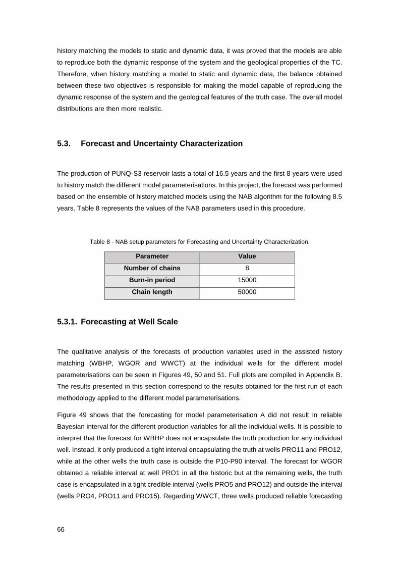
66
history matching the models to static and dynamic data, it was proved that the models are able
to reproduce both the dynamic response of the system and the geological properties of the TC.
Therefore, when history matching a model to static and dynamic data, the balance obtained
between these two objectives is responsible for making the model capable of reproducing the
dynamic response of the system and the geological features of the truth case. The overall model
distributions are then more realistic.
5.3. Forecast and Uncertainty Characterization
The production of PUNQ-S3 reservoir lasts a total of 16.5 years and the first 8 years were used
to history match the different model parameterisations. In this project, the forecast was performed
based on the ensemble of history matched models using the NAB algorithm for the following 8.5
years. Table 8 represents the values of the NAB parameters used in this procedure.
Table 8 - NAB setup parameters for Forecasting and Uncertainty Characterization.
Parameter Value
Number of chains 8
Burn-in period 15000
Chain length 50000
5.3.1. Forecasting at Well Scale
The qualitative analysis of the forecasts of production variables used in the assisted history
matching (WBHP, WGOR and WWCT) at the individual wells for the different model
parameterisations can be seen in Figures 49, 50 and 51. Full plots are compiled in Appendix B.
The results presented in this section correspond to the results obtained for the first run of each
methodology applied to the different model parameterisations.
Figure 49 shows that the forecasting for model parameterisation A did not result in reliable
Bayesian interval for the different production variables for all the individual wells. It is possible to
interpret that the forecast for WBHP does not encapsulate the truth production for any individual
well. Instead, it only produced a tight interval encapsulating the truth at wells PRO11 and PRO12,
while at the other wells the truth case is outside the P10-P90 interval. The forecast for WGOR
obtained a reliable interval at well PRO1 in all the historic but at the remaining wells, the truth
case is encapsulated in a tight credible interval (wells PRO5 and PRO12) and outside the interval
(wells PRO4, PRO11 and PRO15). Regarding WWCT, three wells produced reliable forecasting
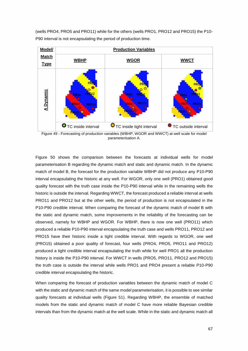
67
(wells PRO4, PRO5 and PRO11) while for the others (wells PRO1, PRO12 and PRO15) the P10-
P90 interval is not encapsulating the period of production time.
Model/
Match
Type
Production Variables
WBHP WGOR WWCT
A D
yn
am
ic
TC inside interval TC inside tight interval TC outside interval
Figure 49 - Forecasting of production variables (WBHP, WGOR and WWCT) at well scale for model
parameterisation A.
Figure 50 shows the comparison between the forecasts at individual wells for model
parameterisation B regarding the dynamic match and static and dynamic match. In the dynamic
match of model B, the forecast for the production variable WBHP did not produce any P10-P90
interval encapsulating the historic at any well. For WGOR, only one well (PRO1) obtained good
quality forecast with the truth case inside the P10-P90 interval while in the remaining wells the
historic is outside the interval. Regarding WWCT, the forecast produced a reliable interval at wells
PRO11 and PRO12 but at the other wells, the period of production is not encapsulated in the
P10-P90 credible interval. When comparing the forecast of the dynamic match of model B with
the static and dynamic match, some improvements in the reliability of the forecasting can be
observed, namely for WBHP and WGOR. For WBHP, there is now one well (PRO11) which
produced a reliable P10-P90 interval encapsulating the truth case and wells PRO11, PRO12 and
PRO15 have their historic inside a tight credible interval. With regards to WGOR, one well
(PRO15) obtained a poor quality of forecast, four wells (PRO4, PRO5, PRO11 and PRO12)
produced a tight credible interval encapsulating the truth while for well PRO1 all the production
history is inside the P10-P90 interval. For WWCT in wells (PRO5, PRO11, PRO12 and PRO15)
the truth case is outside the interval while wells PRO1 and PRO4 present a reliable P10-P90
credible interval encapsulating the historic.
When comparing the forecast of production variables between the dynamic match of model C
with the static and dynamic match of the same model parameterisation, it is possible to see similar
quality forecasts at individual wells (Figure 51). Regarding WBHP, the ensemble of matched
models from the static and dynamic match of model C have more reliable Bayesian credible
intervals than from the dynamic match at the well scale. While in the static and dynamic match all
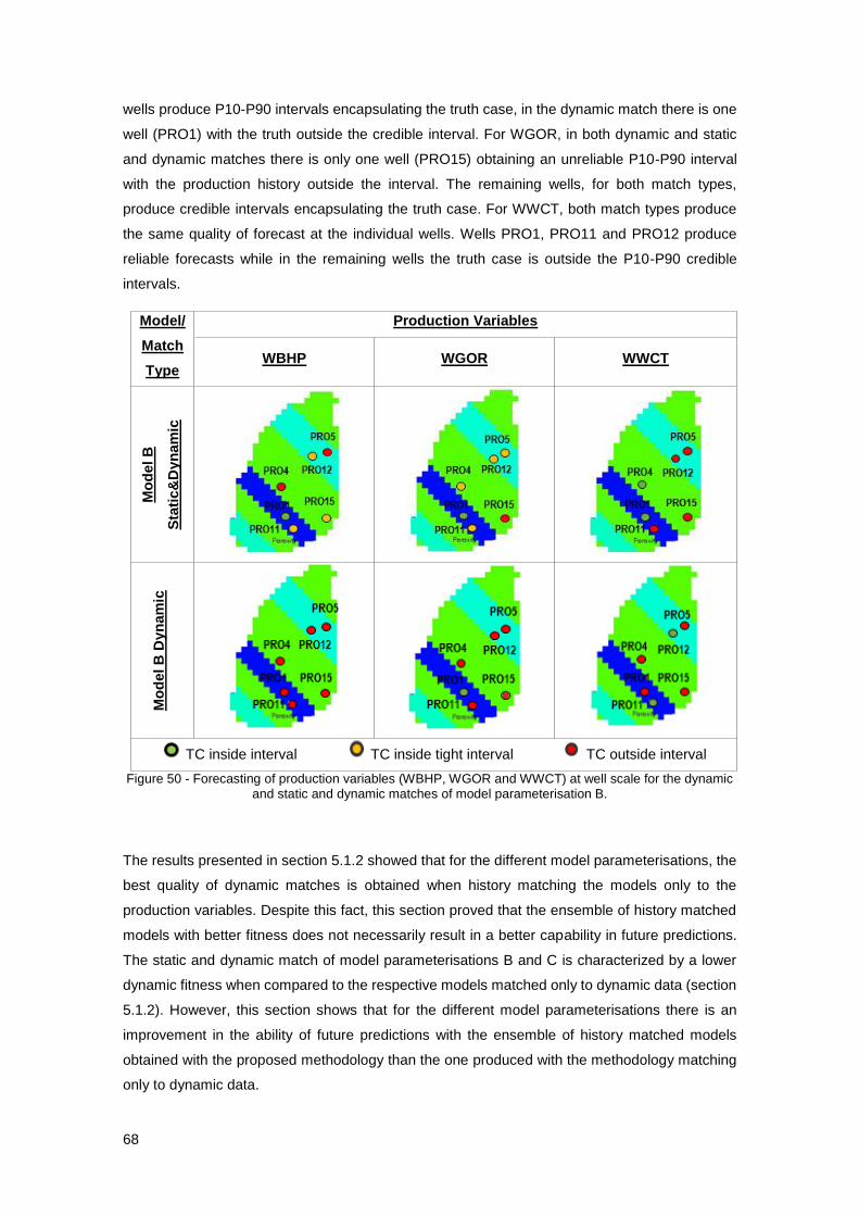
68
wells produce P10-P90 intervals encapsulating the truth case, in the dynamic match there is one
well (PRO1) with the truth outside the credible interval. For WGOR, in both dynamic and static
and dynamic matches there is only one well (PRO15) obtaining an unreliable P10-P90 interval
with the production history outside the interval. The remaining wells, for both match types,
produce credible intervals encapsulating the truth case. For WWCT, both match types produce
the same quality of forecast at the individual wells. Wells PRO1, PRO11 and PRO12 produce
reliable forecasts while in the remaining wells the truth case is outside the P10-P90 credible
intervals.
Model/
Match
Type
Production Variables
WBHP WGOR WWCT
Mo
del B
Sta
tic&
Dyn
am
ic
Mo
del B
Dyn
am
ic
TC inside interval TC inside tight interval TC outside interval
Figure 50 - Forecasting of production variables (WBHP, WGOR and WWCT) at well scale for the dynamic and static and dynamic matches of model parameterisation B.
The results presented in section 5.1.2 showed that for the different model parameterisations, the
best quality of dynamic matches is obtained when history matching the models only to the
production variables. Despite this fact, this section proved that the ensemble of history matched
models with better fitness does not necessarily result in a better capability in future predictions.
The static and dynamic match of model parameterisations B and C is characterized by a lower
dynamic fitness when compared to the respective models matched only to dynamic data (section
5.1.2). However, this section shows that for the different model parameterisations there is an
improvement in the ability of future predictions with the ensemble of history matched models
obtained with the proposed methodology than the one produced with the methodology matching
only to dynamic data.

69
Model/
Match
Type
Production Variables
WBHP WGOR WWCT M
od
el C
Sta
tic&
Dyn
am
ic
Mo
del C
Dyn
am
ic
TC inside interval TC inside tight interval TC outside interval
Figure 51 - Forecasting of production variables (WBHP, WGOR and WWCT) at well scale for the dynamic and static and dynamic matches of model parameterisation C.
History matching a model to static and dynamic data, not only produces an ensemble of history
matched models with the ability of reproducing the historical production and characterized by
overall distributions more realistic but also improves the capability and reliability when forecasting
the response of the system.
5.3.2. Forecasting at Field Scale
This subsection presents the results obtained in forecasting the field oil production total (FOPT)
and field water production total (FWPT) for the different model parameterisations (Figures 52, 53
and 54).
Figure 52 shows the uncertainty quantification in forecasting total oil and water recovery of the
entire life of the field for model A. It is possible to see that for both FOPT and FWPT the truth
case is encapsulated in the reliable Bayesian credible interval. Furthermore, the P50 value in this
run for both oil and water recovery is also close to the truth case value at the end of production.
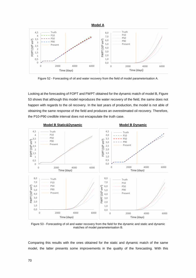
70
Model A
Figure 52 - Forecasting of oil and water recovery from the field of model parameterisation A.
Looking at the forecasting of FOPT and FWPT obtained for the dynamic match of model B, Figure
53 shows that although this model reproduces the water recovery of the field, the same does not
happen with regards to the oil recovery. In the last years of production, the model is not able of
obtaining the same response of the field and produces an overestimated oil recovery. Therefore,
the P10-P90 credible interval does not encapsulate the truth case.
Model B Static&Dynamic Model B Dynamic
Figure 53 - Forecasting of oil and water recovery from the field for the dynamic and static and dynamic matches of model parameterisation B.
Comparing this results with the ones obtained for the static and dynamic match of the same
model, the latter presents some improvements in the quality of the forecasting. With this
0
0,5
1
1,5
2
2,5
3
3,5
4
4,5
0 2000 4000 6000
FOP
T (1
06
sm3 )
Time (days)
TruthP10P50P90Present
0,0
1,0
2,0
3,0
4,0
5,0
6,0
7,0
8,0
0 2000 4000 6000
FWP
T (1
05
sm3)
Time (days)
TruthP10P50P90Present
0
0,5
1
1,5
2
2,5
3
3,5
4
4,5
0 2000 4000 6000
FOP
T (1
06
sm3 )
Time (days)
TruthP10P50P90Present
0,0
0,5
1,0
1,5
2,0
2,5
3,0
3,5
4,0
4,5
0 2000 4000 6000
FOP
T (1
06
sm3 )
Time (days)
TruthP10P50P90Present
0,0
1,0
2,0
3,0
4,0
5,0
6,0
7,0
8,0
0 2000 4000 6000
FWP
T (1
05
sm3)
Time (days)
Truth
P10
P50
P90
Present
0,0
1,0
2,0
3,0
4,0
5,0
6,0
7,0
8,0
0 2000 4000 6000
FWP
T (1
05
sm3)
Time (days)
Truth
P10
P50
P90
Present
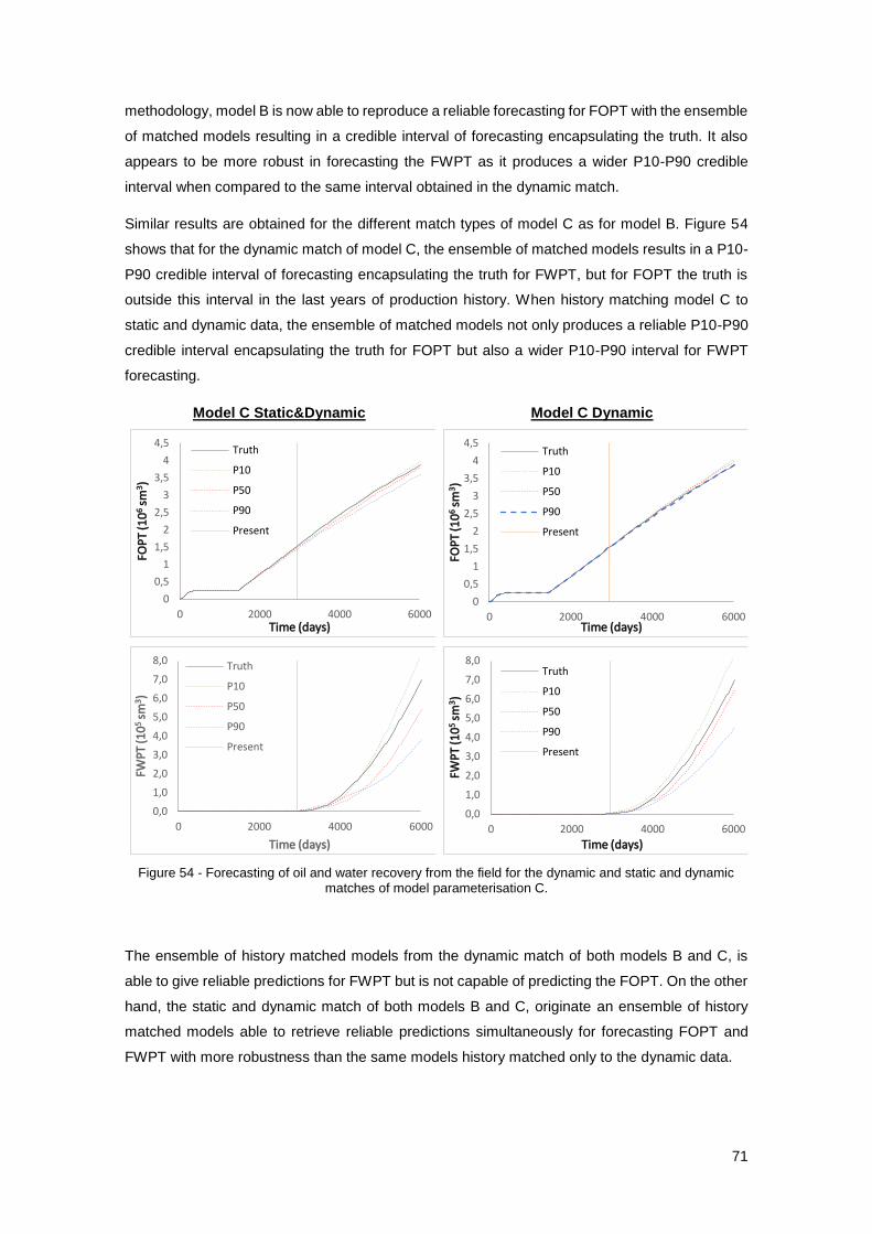
71
methodology, model B is now able to reproduce a reliable forecasting for FOPT with the ensemble
of matched models resulting in a credible interval of forecasting encapsulating the truth. It also
appears to be more robust in forecasting the FWPT as it produces a wider P10-P90 credible
interval when compared to the same interval obtained in the dynamic match.
Similar results are obtained for the different match types of model C as for model B. Figure 54
shows that for the dynamic match of model C, the ensemble of matched models results in a P10-
P90 credible interval of forecasting encapsulating the truth for FWPT, but for FOPT the truth is
outside this interval in the last years of production history. When history matching model C to
static and dynamic data, the ensemble of matched models not only produces a reliable P10-P90
credible interval encapsulating the truth for FOPT but also a wider P10-P90 interval for FWPT
forecasting.
Model C Static&Dynamic Model C Dynamic
Figure 54 - Forecasting of oil and water recovery from the field for the dynamic and static and dynamic matches of model parameterisation C.
The ensemble of history matched models from the dynamic match of both models B and C, is
able to give reliable predictions for FWPT but is not capable of predicting the FOPT. On the other
hand, the static and dynamic match of both models B and C, originate an ensemble of history
matched models able to retrieve reliable predictions simultaneously for forecasting FOPT and
FWPT with more robustness than the same models history matched only to the dynamic data.
0
0,5
1
1,5
2
2,5
3
3,5
4
4,5
0 2000 4000 6000
FOP
T (1
06
sm3 )
Time (days)
Truth
P10
P50
P90
Present
0
0,5
1
1,5
2
2,5
3
3,5
4
4,5
0 2000 4000 6000
FOP
T (1
06
sm3 )
Time (days)
Truth
P10
P50
P90
Present
0,0
1,0
2,0
3,0
4,0
5,0
6,0
7,0
8,0
0 2000 4000 6000
FWP
T (1
05
sm3)
Time (days)
Truth
P10
P50
P90
Present
0,0
1,0
2,0
3,0
4,0
5,0
6,0
7,0
8,0
0 2000 4000 6000
FWP
T (1
05
sm3)
Time (days)
Truth
P10
P50
P90
Present

72
These results suggest that history matching a model to static and dynamic data originate an
ensemble of matched models that give predictions with more reliability and robustness than the
ensemble of history matched models generated in the dynamic match.
The different model parameterisations originated different predictions for cumulative oil and water
production. Bayesian Model Averaging (section 2.5.2) was then used to combine these
predictions from model parameterisations A, B Sta&Dyn and C Sta&Dyn into a global prediction,
based in the dynamic likelihood and the static and dynamic likelihood. The results presented
correspond to the results obtained for the first run applied to these different model
parameterisations.
Model parameterisation C Sta&Dyn presents the maximum dynamic likelihood achieved by
iteration 192 and so is considered the reference model for calculating Normalised Bayes Factor
(BF) shown in Figure 55. The BF results show that model descriptions A and B Sta&Dyn, 0.0269
and 0.1448 respectively, have only a small part of the reference model which is due to the
differences between their maximum dynamic likelihoods (0.004469 for model A, 0.018474 for
model B and 0.095741 for model C).
Figure 55 - Normalised Bayes Factors of model parameterisations A, B Sta&Dyn and C Sta&Dyn based in the dynamic likelihood.
The PDF of the different models in a moment in time can be averaged to obtain a new probability
curve, using the corresponding BF. The average Cumulative Distribution Function (CDF) for the
last timestep of the forecasting period of FOPT and FWPT with the new P10, P50 and P90 values
are presented in Figure 56. From Figure 56 it is possible to see that the new CDF for both FOPT
and FWPT follows almost exactly the CDF of model C. These results can also be seen in Figure
57 where the uncertainty envelope for the BMA is plotted together with the original uncertainty
envelopes of the different model descriptions. The averaged uncertainty envelope of FOPT
(362522.09 sm3) encompasses part of the envelope of model A (260961.19), all envelope of
model B (198620.23 sm3) and almost all of model C (367892.92 sm3). Regarding the averaged
uncertainty envelope for FWPT (259784.67 sm3), it overlaps all envelope of model C (229856.36
sm3) disregarding most of the envelopes of models A and B (512701.13 sm3 and 490906.61 sm3,
respectively).
0
0,2
0,4
0,6
0,8
1
A B Sta&Dyn C Sta&Dyn
No
rmal
ized
Bay
es F
acto
r
Dynamic
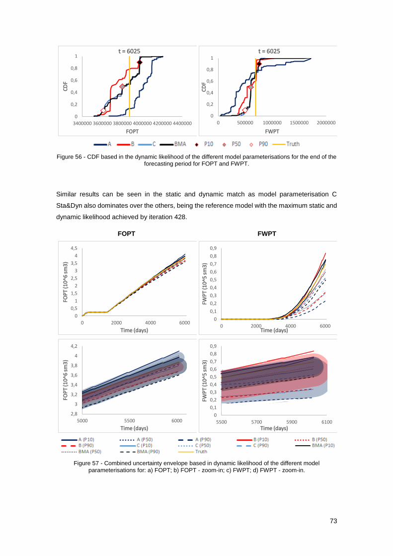
73
Figure 56 - CDF based in the dynamic likelihood of the different model parameterisations for the end of the forecasting period for FOPT and FWPT.
Similar results can be seen in the static and dynamic match as model parameterisation C
Sta&Dyn also dominates over the others, being the reference model with the maximum static and
dynamic likelihood achieved by iteration 428.
FOPT FWPT
Figure 57 - Combined uncertainty envelope based in dynamic likelihood of the different model
parameterisations for: a) FOPT; b) FOPT - zoom-in; c) FWPT; d) FWPT - zoom-in.
0
0,2
0,4
0,6
0,8
1
3400000 3600000 3800000 4000000 4200000 4400000
CD
F
FOPT
t = 6025
0
0,2
0,4
0,6
0,8
1
0 500000 1000000 1500000 2000000
CD
F
FWPT
t = 6025
0
0,5
1
1,5
2
2,5
3
3,5
4
4,5
0 2000 4000 6000
FOP
T (1
0^6
sm
3)
Time (days)
0
0,1
0,2
0,3
0,4
0,5
0,6
0,7
0,8
0,9
0 2000 4000 6000
FWP
T (1
0^5
sm
3)
Time (days)
2,8
3
3,2
3,4
3,6
3,8
4
4,2
5000 5500 6000
FOP
T (1
0^6
sm
3)
Time (days)
0
0,1
0,2
0,3
0,4
0,5
0,6
0,7
0,8
0,9
5500 5700 5900 6100
FWP
T (1
0^5
sm
3)
Time (days)
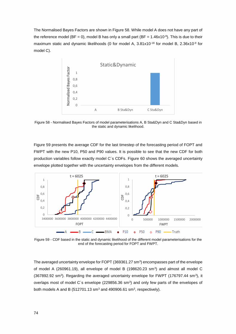
74
The Normalised Bayes Factors are shown in Figure 58. While model A does not have any part of
the reference model (BF = 0), model B has only a small part (BF = 1.46x10⁻⁹). This is due to their
maximum static and dynamic likelihoods (0 for model A, 3.81x10⁻¹⁸ for model B, 2.36x10⁻⁹ for
model C).
Figure 58 - Normalised Bayes Factors of model parameterisations A, B Sta&Dyn and C Sta&Dyn based in the static and dynamic likelihood.
Figure 59 presents the average CDF for the last timestep of the forecasting period of FOPT and
FWPT with the new P10, P50 and P90 values. It is possible to see that the new CDF for both
production variables follow exactly model C´s CDFs. Figure 60 shows the averaged uncertainty
envelope plotted together with the uncertainty envelopes from the different models.
Figure 59 - CDF based in the static and dynamic likelihood of the different model parameterisations for the end of the forecasting period for FOPT and FWPT.
The averaged uncertainty envelope for FOPT (369361.27 sm3) encompasses part of the envelope
of model A (260961.19), all envelope of model B (198620.23 sm3) and almost all model C
(367892.92 sm3). Regarding the averaged uncertainty envelope for FWPT (176797.44 sm3), it
overlaps most of model C´s envelope (229856.36 sm3) and only few parts of the envelopes of
both models A and B (512701.13 sm3 and 490906.61 sm3, respectively).
0
0,2
0,4
0,6
0,8
1
A B Sta&Dyn C Sta&Dyn
No
rmal
ized
Bay
es F
acto
r Static&Dynamic
0
0,2
0,4
0,6
0,8
1
3400000 3600000 3800000 4000000 4200000 4400000
CD
F
FOPT
t = 6025
0
0,2
0,4
0,6
0,8
1
0 500000 1000000 1500000 2000000
CD
F
FWPT
t = 6025

75
Figure 61 shows the average of credible interval (P10-P50-P90) in forecasting of total oil recovery
at the end of production of the field over 5 runs from the different types of matches of the different
model parameterisations. For terms of comparison, the uncertainty envelope obtained in the BMA
based on both likelihoods (dynamic and static and dynamic) as well as the uncertainty envelope
of the True geostatistical model related to the random seed are also presented in the Figure.
FOPT FWPT
Figure 60 - Combined uncertainty envelope based in the static and dynamic likelihood of the different model parameterisations for: a) FOPT; b) FOPT - zoom-in; c) FWPT; d) FWPT - zoom-in.
From the Figure 61 it is possible to infer that except for B Dyn model parameterisation, the
forecasts from both type of matches of the different model parameterisations are reliable as the
credible interval encapsulates the truth value. The credible interval obtained for the history
matched models to static and dynamic data is more reliable and robust than the intervals obtained
from the same models only matched to dynamic data. Moreover, under different
parameterisations the mean value of each credible interval in forecasting from the ensemble of
history matched models obtained with the proposed methodology is comparable, while from the
ensemble produced in the dynamic match is collapsed to different range of credible interval.
The uncertainty envelopes obtained in the BMA based in both dynamic and static and dynamic
likelihoods are also reliable and robust. The truth is encapsulated in the P10-P90 intervals and
their mean P50 is similar to the truth history. The different BMA envelopes are resemblant and
0
0,5
1
1,5
2
2,5
3
3,5
4
4,5
0 2000 4000 6000
FOP
T (1
0^6
sm
3)
Time (days)
0
0,1
0,2
0,3
0,4
0,5
0,6
0,7
0,8
0,9
0 2000 4000 6000FW
PT
(10
^5 s
m3
)Time (days)
2,8
3
3,2
3,4
3,6
3,8
4
4,2
5000 5500 6000
FOP
T (1
0^6
sm
3)
Time (days)
0
0,1
0,2
0,3
0,4
0,5
0,6
0,7
0,8
0,9
5500 5700 5900 6100
FWP
T (1
0^5
sm
3)
Time (days)

76
comparable to the credible interval from the static and dynamic match of model C as this model
is characterized by both maximum dynamic and static and dynamic likelihoods.
Figure 61 - Average of credible interval (P10-P50-P90) in forecasting of oil recovery at the end of production from the field of the different model parameterisations, BMA based in dynamic and static and
dynamic likelihoodds and True geostatistical model related to the random seed.
Among the different P10-P90 intervals obtained from the different model parameterisations, the
one obtained from model description C Sta&Dyn not only produces a mean P50 closer to the truth
history value but also has a range of uncertainty comparable with the stochastic uncertainty
associated with the True geostatistical model related to the random seed.
5.3.3. Comparing overall forecasting at individual well
Figure 62 presents the comparison between model parameterisations A, B Sta&Dyn and C
Sta&Dyn of the truth case falling into the credible interval (CI) regarding the different production
variables for each individual well. The results obtained for both BMA based in dynamic and static
and dynamic likelihoods are also presented in the Figure.
In Figure 62, the wells are considered to have the truth case within the credible interval (green) if
the P10-P90 interval encapsulates the truth historic for the different production variables during
all forecasting period. The wells are considered to have the TC mostly within the CI (yellow) if the
truth historic regarding GOR, BHP and WCT is encapsulated in the credible interval during most
of the forecasting period. If the P10-P90 interval for the different production variables only
encapsulates parts of the truth history during all timesteps of forecasting, the wells are considered
3,3
3,4
3,5
3,6
3,7
3,8
3,9
4
4,1
4,2
4,3
A B Dyn B Sta&Dyn C Dyn C Sta&Dyn BMA Dyn BMASta&Dyn
True Geost.Model
FOP
T (1
0^6
sm
3)
P10 P50 P90 Truth
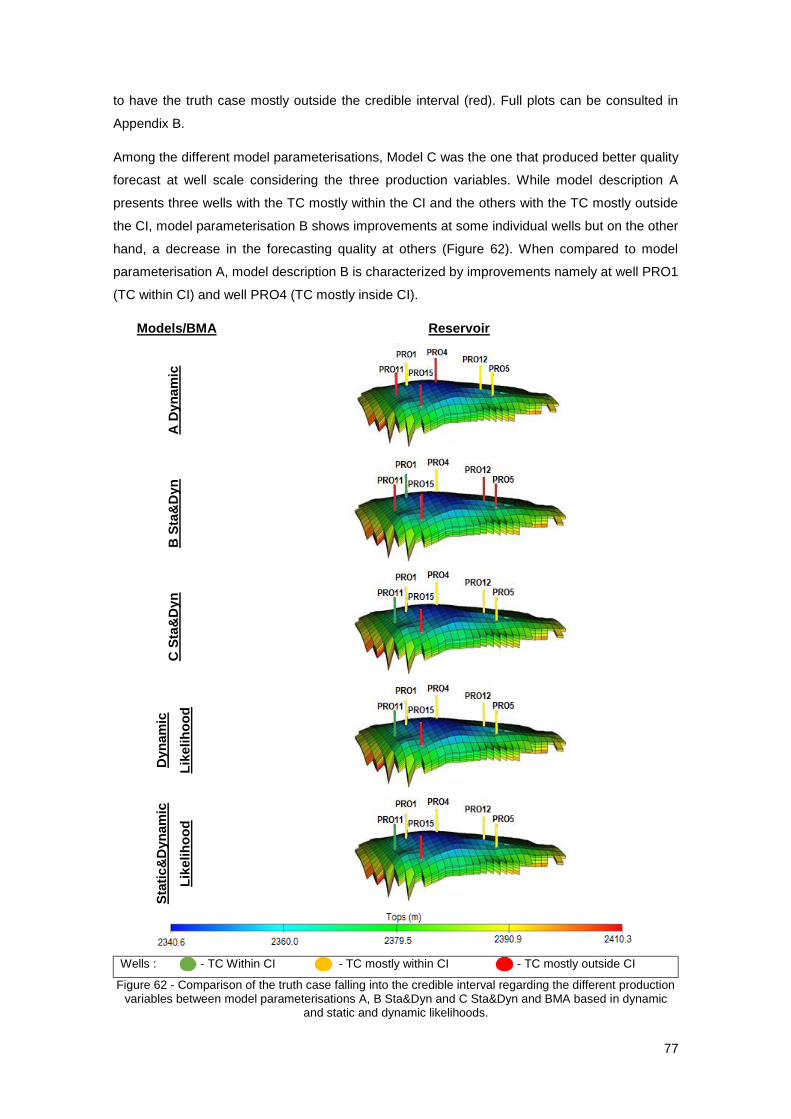
77
to have the truth case mostly outside the credible interval (red). Full plots can be consulted in
Appendix B.
Among the different model parameterisations, Model C was the one that produced better quality
forecast at well scale considering the three production variables. While model description A
presents three wells with the TC mostly within the CI and the others with the TC mostly outside
the CI, model parameterisation B shows improvements at some individual wells but on the other
hand, a decrease in the forecasting quality at others (Figure 62). When compared to model
parameterisation A, model description B is characterized by improvements namely at well PRO1
(TC within CI) and well PRO4 (TC mostly inside CI).
Models/BMA Reservoir
A D
yn
am
ic
B S
ta&
Dyn
C S
ta&
Dyn
Dyn
am
ic
Lik
elih
oo
d
Sta
tic&
Dyn
am
ic
Lik
elih
oo
d
Wells : - - TC Within CI - TC mostly within CI - TC mostly outside CI
Figure 62 - Comparison of the truth case falling into the credible interval regarding the different production variables between model parameterisations A, B Sta&Dyn and C Sta&Dyn and BMA based in dynamic
and static and dynamic likelihoods.
78
In model description A, regarding BHP at well PRO1 the truth historic is encapsulated in the P10-
P90 interval only at the end of the forecasting period and for GOR the credible interval
encapsulates the truth historic at all period of the forecasting (Appendix B – Figure B.1). In model
parameterisation B not only the history of the same production variables at the same well is within
the credible interval as the same happens regarding WCT (Appendix B – Figure B.3). Well PRO4
in model A only for WCT has the history inside the Bayesian interval (Appendix B – Figure B.1)
while in model description B it has also parts of the truth history of BHP and GOR inside the CI
(Appendix B – Figure B.3), namely for the last timesteps of the forecasting period. When it comes
to wells PRO5 and PRO12 (Appendix B – Figure B.1), in model parameterisation A all the
production variables have the truth history inside the CI at some timesteps of the forecasting
period. For model description B the same does not happen, namely for BHP at well PRO5 and
WCT at well PRO12 (Appendix B – Figure B.3). Regarding wells PRO11 and PRO15, the truth
history is mainly outside the P10-P90 interval for both model parameterisations A and B regarding
the three production variables (Appendix B – Figures B.1 and B.3).
Model description C, when compared to the other model parameterisations, presents
improvements in the quality of forecasting at each well, being the exception well PRO1. For wells
PRO1, PRO4, PRO5 and PRO12, the historical production during almost all forecasting period is
enclosed in the P10-P90 interval regarding the different production variables (Appendix B –
Figures B.5). Well PRO11 is characterized by the best quality of forecasting with the TC within
the CI for the three production variables at all timesteps (Appendix B – Figure B.5). The poorest
quality of forecasting can be found at well PRO15, where GOR has the truth history enclosed in
the P10-P90 interval only at the beginning of the forecasting period and the WCT production
history is outside the credible interval for the entire period of forecasting (Appendix B – Figure
B.5).
For both BMA based in dynamic and static and dynamic likelihoods the truth case falling into the
credible interval at each individual well outcomes similar to model C as this model is characterized
by the highest likelihoods when compared with the others. For the BMA based in static and
dynamic likelihood the forecasting of the different production variables at individual well is almost
exactly similar to model C (Appendix B – Figure B.7). For the BMA based in dynamic likelihood,
although it is similar and follows the same trend as in model C, there are some differences at
particular wells and variables. When compared to model C, well PRO1 in the BMA based on
dynamic likelihood presents a wider credible interval during all forecasting period regarding BHP
(Appendix B – Figure B.6). For GOR and WCT it is also wider but specially at the last timesteps
of forecasting (Appendix B – Figure B.6). Well PRO4 also shows a larger CI for GOR during the
entire period of forecasting and for WCT, it is wider but only until the first half of forecasting
(Appendix B – Figure B.6). Regarding well PRO5, for both BHP and WCT the P10-P90 interval is
larger during all timesteps of forecasting (Appendix B – Figure B.6). WCT at well PRO11 is the
only production variable presenting a wider CI (Appendix B – Figure B.6).
79
6. Conclusions
Over the last years the history matching has been approached by multi-objective optimisation
powered by stochastic population-based algorithms. This approach provides a more diverse set
of matched models leading to a better production forecast and uncertainty quantification. These
techniques have been applied exclusively by matching multiple production variables from the
historical production data of the reservoir. However, due to the nature of history matching
problems, the fact that a reservoir model reproduces the dynamic response of the system does
not necessarily mean it is respecting the geological characteristics from the field.
The methodology proposed under the scope of this thesis entails history matching the reservoir
model through the application of a multi-objective optimisation approach, not only by matching
the production data but also the petrophysical properties at the well locations. Different model
parameterisations, which represent different geological uncertainty in the reservoir, were studied.
For terms of comparison, the different model parameterisations were also history matched using
a multi-objective optimisation approach to obtain exclusively the match to production data.
Under different model parameterisations (A, B and C) both methodologies showed good ability to
generate Pareto Models able to reproduce the dynamic response of the truth case. Using the
methodology to obtain only the dynamic match, the different model parameterisations presented
very good quality matches to the different production variables at well scale. Although the quality
of the dynamic matches decreased when using the proposed approach, the obtained Pareto
Models are also characterized by overall good quality matches at individual well and therefore,
able of reproducing the historical production of the reservoir.
Regarding the quality of the matches to the petrophysical properties at well scale, it was possible
to see some improvements in the quality of the results when comparing the Pareto Models
obtained from the proposed methodology with the ones generated from the methodology to obtain
exclusively the dynamic match. The Pareto Models generated from the different model
parameterisations history matched with the methodology to obtain the dynamic match are
featured by poor quality static matches at the different wells. On the other hand, history matching
model parameterisations B and C with the proposed methodology generated Pareto Models
capable of reproducing the geological characteristics of the different facies types. The static and
dynamic match of model C presents the best results when compared to the others. This model is
parameterised with similar prior distributions to the truth case and the new zone orientation model
has also impact in the quality of the static matches, especially in layers 1, 3 and 5 (fluvial channel
fills and floodplain mudstones facies types). Only the Pareto Models obtained from the static and
dynamic match of model C are characterized by Phi/PermX and PermX/PermZ joint distributions
concordant with the correlations of the truth case allowing to infer realistic overall model
distributions. The Pareto Models of the different model parameterisations obtained from the
80
methodology for the dynamic match do not show the same joint distribution as the truth case and
therefore are geologically inconsistent.
The ensemble of history matched models obtained when history matching model
parameterisations B and C with the proposed methodology is capable of giving reliable production
predictions at both well and field scale. When compared to the ensemble of history matched
models from the methodology to obtain the dynamic match, the ensemble from the proposed
methodology is characterized by more wells located within the Bayesian plausible interval for the
different production variables. Both FOPT and FWPT are also predicted with a P10-P90 interval
more reliable and robust. It was proved that adding static data to the history matching has impact
in predicting the cumulative oil production rather than cumulative water production. It was also
proved that forecasting the production uncertainty range with a simple multiplier model with basic
geology produces a P10-P50-P90 credible interval comparable to the uncertainty associated with
the True geostatistical model related to the random seed.
Using the Bayesian Model Averaging to combine the uncertainty envelopes of FOPT and FWPT
of model parameterisations A, B Sta&Dyn and C Sta&Dyn based in both dynamic and static and
dynamic likelihoods showed that model C dominates over the others. The combined uncertainty
envelope of cumulative oil and water productions based in both likelihoods, encompasses and
follows almost exactly the uncertainty envelopes of model C disregarding the ones from the other
models.
The best quality of overall forecasting at well scale is found in the static and dynamic match of
model parameterisation C. When compared with the other model descriptions, model C evidences
more wells with the ability to give reliable predictions regarding the different production variables.
As model parameterisation C is characterized by the maximum dynamic and static and dynamic
likelihoods, the BMAs based in both likelihoods are resemblant. BMA based in static and dynamic
likelihood presents similar credible intervals for the three production variables at the different
wells. BMA based in dynamic likelihood is also similar and follows the same trend but has larger
P10-P90 intervals for some variables at particular wells.
81
References
Arnold, D., Demyanov, V., D. Tatum, Christie, M., Rojas, T., Geiger, S., Corbett, P. 2013.
Hierarchical benchmark case study for history matching, uncertainty quantification and reservoir
characterization, Elsevier;
Barwis; J.H., McPherson, J.G., Studlick, J.R.J. 1990. Sandstone Petroleum Reservoirs. Springer-
Verlag, New York inc.;
Christie, M. 1996. Upscaling for Reservoir Simulation. Journal of Petroleum Technology. 48 (11):
1004-1010.
Christie, M., Demyanov, V., Erbas, D. 2006. Uncertainty quantification for porous media flows,
Elsevier, Journal of Computational Physics 217;
Christie, M., Demyanov, V, Eydinov, D. 2013. Use of Multi-Objective Algorithms in History
Matching of a Real Field. Presented at SPE Reservoir Simulation Symposium, Woodlands,
Texas, USA, 18-20 February;
Christie, M.A., Glimm, J., Grove, J.W., Higdon, D.M., Sharp, D.H., Wood-Schultz, M.M. 2005.
Error analysis and simulations of complex phenomena. Los Alamos Science 29, 6–25;
Cosentino, L. 2001. Integrated Reservoir Studies, Editions Technip;
Erbas, D., Christie, M. 2007. Effect of Sampling Strategies on Prediction Uncertainty Estimation,
paper 106229. Presented at SPE Reservoir Simulation Symposium, Houston, Texas, U.S.A, 26-
28 February;
Ferraro, P., Verga, F. 2009. Use of evolutionary algorithms in single and multi-objective
Optimisation techniques for assisted history matching. Presented at the OMC&E, Ravenna, Italy,
25-27 March;
Floris, F., Bush, M., Cuypers, M., Roggero, F., Syversveen, A. 2001. Methods for quantifying the
uncertainty of production forecasts – a comparative study. Petroleum Geoscience, 7, 587-596;
Galloway, W.E., Hobday, D.K. 1983. Terrigenous Clastic Depositional Systems, Applications to
Petroleum, Coal, and Uranium Exploration. Springer-Verlag.
Gilman, J., Ozgen, C. 2013. Reservoir Simulation: History Matching and Forecasting, Society of
Petroleum Engineers;
Grundvag, S.A., Hansen, W.H., Johannessen, E.P., Olsen, A.H., Stene, S.A.K. 2014. The
depositional architecture and fácies variability of shelf deltas in the Eocene Battfjellet Formation,
Nathorst Land, Spitsbergen. Sedimentology, 61, 2172-2204;
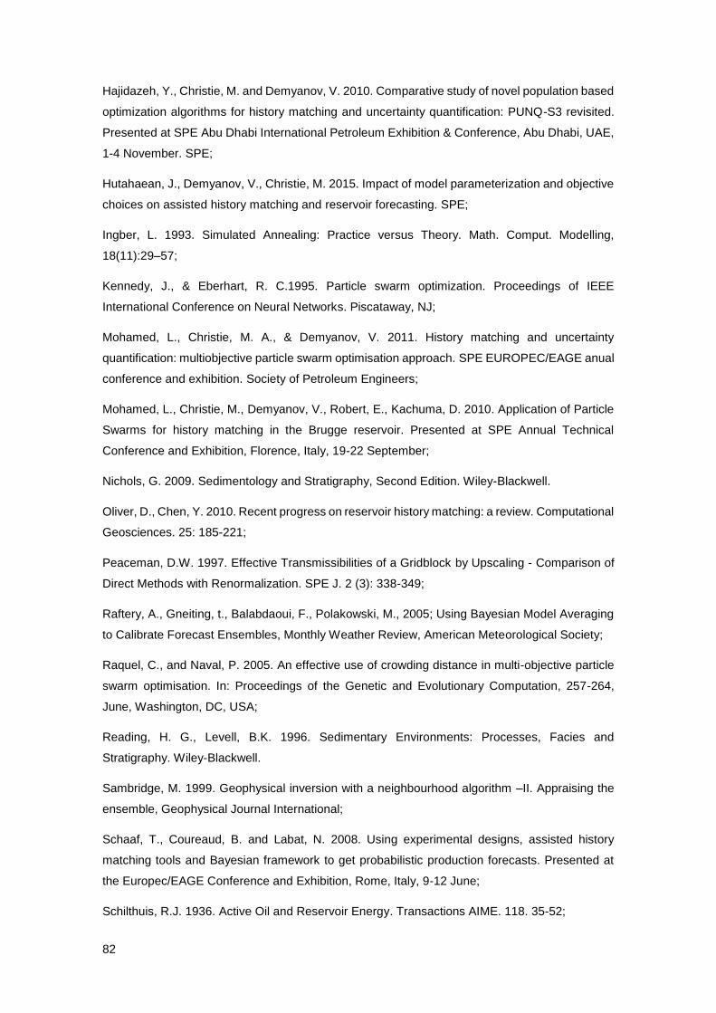
82
Hajidazeh, Y., Christie, M. and Demyanov, V. 2010. Comparative study of novel population based
optimization algorithms for history matching and uncertainty quantification: PUNQ-S3 revisited.
Presented at SPE Abu Dhabi International Petroleum Exhibition & Conference, Abu Dhabi, UAE,
1-4 November. SPE;
Hutahaean, J., Demyanov, V., Christie, M. 2015. Impact of model parameterization and objective
choices on assisted history matching and reservoir forecasting. SPE;
Ingber, L. 1993. Simulated Annealing: Practice versus Theory. Math. Comput. Modelling,
18(11):29–57;
Kennedy, J., & Eberhart, R. C.1995. Particle swarm optimization. Proceedings of IEEE
International Conference on Neural Networks. Piscataway, NJ;
Mohamed, L., Christie, M. A., & Demyanov, V. 2011. History matching and uncertainty
quantification: multiobjective particle swarm optimisation approach. SPE EUROPEC/EAGE anual
conference and exhibition. Society of Petroleum Engineers;
Mohamed, L., Christie, M., Demyanov, V., Robert, E., Kachuma, D. 2010. Application of Particle
Swarms for history matching in the Brugge reservoir. Presented at SPE Annual Technical
Conference and Exhibition, Florence, Italy, 19-22 September;
Nichols, G. 2009. Sedimentology and Stratigraphy, Second Edition. Wiley-Blackwell.
Oliver, D., Chen, Y. 2010. Recent progress on reservoir history matching: a review. Computational
Geosciences. 25: 185-221;
Peaceman, D.W. 1997. Effective Transmissibilities of a Gridblock by Upscaling - Comparison of
Direct Methods with Renormalization. SPE J. 2 (3): 338-349;
Raftery, A., Gneiting, t., Balabdaoui, F., Polakowski, M., 2005; Using Bayesian Model Averaging
to Calibrate Forecast Ensembles, Monthly Weather Review, American Meteorological Society;
Raquel, C., and Naval, P. 2005. An effective use of crowding distance in multi-objective particle
swarm optimisation. In: Proceedings of the Genetic and Evolutionary Computation, 257-264,
June, Washington, DC, USA;
Reading, H. G., Levell, B.K. 1996. Sedimentary Environments: Processes, Facies and
Stratigraphy. Wiley-Blackwell.
Sambridge, M. 1999. Geophysical inversion with a neighbourhood algorithm –II. Appraising the
ensemble, Geophysical Journal International;
Schaaf, T., Coureaud, B. and Labat, N. 2008. Using experimental designs, assisted history
matching tools and Bayesian framework to get probabilistic production forecasts. Presented at
the Europec/EAGE Conference and Exhibition, Rome, Italy, 9-12 June;
Schilthuis, R.J. 1936. Active Oil and Reservoir Energy. Transactions AIME. 118. 35-52;

83
Schulze-Riegert, R.W., Axmann, J.K., Haase, O., Rian, D.T., You, Y. 2001. Optimisation Methods
for History Matching of Complex Reservoirs, paper 66393. Presented at SPE Reservoir
Simulation Symposium, Houston, Texas, U.S.A, 11-14 February;
Schulze-Riegert, R., Krosche, M., Fahimuddin, A, Ghedan, S. 2007. Multi-objective optimisation
with application to model validation and uncertainty quantification. Presented at 15th SPE Middle
East Oil and Gas Show and Conference, Bahrain, 11-14 March;
Tarantola, A. 2005. Inverse Problem Theory and Methods for Modelling Parameters Estimation.
Society for Industrial and Applied Mathematics. Philadelphia. 342 pp;
Tavassoli, Z., Carter, J., King, P. 2004. Errors in History Matching, September 2004 SPE Journal.

84
This page intentionally left blank
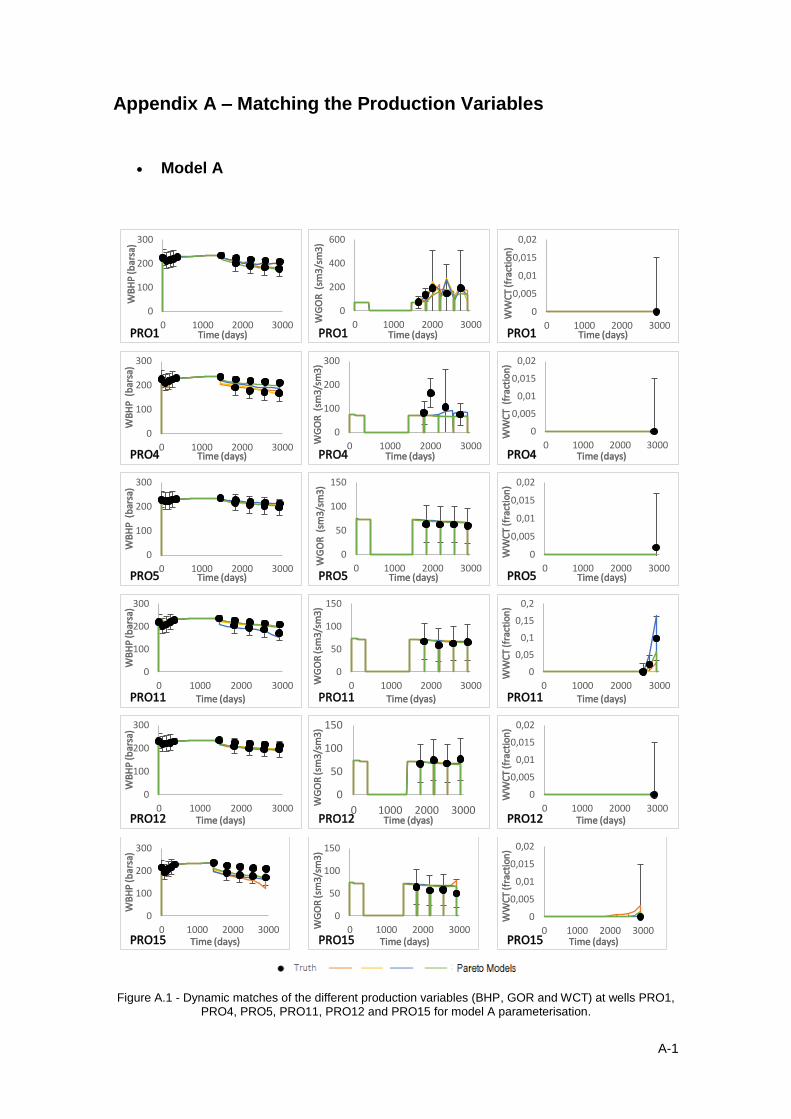
A-1
Appendix A – Matching the Production Variables
• Model A
Figure A.1 - Dynamic matches of the different production variables (BHP, GOR and WCT) at wells PRO1, PRO4, PRO5, PRO11, PRO12 and PRO15 for model A parameterisation.
0
100
200
300
0 1000 2000 3000
WB
HP
(bar
sa)
Time (days)PRO1
0
200
400
600
0 1000 2000 3000WG
OR
(sm
3/sm
3)
Time (days)PRO1
0
0,005
0,01
0,015
0,02
0 1000 2000 3000
WW
CT
(fra
ctio
n)
Time (days)PRO1
0
100
200
300
0 1000 2000 3000
WB
HP
(b
arsa
)
Time (days)PRO4
0
100
200
300
0 1000 2000 3000WG
OR
(sm
3/sm
3)
Time (days)PRO4
0
0,005
0,01
0,015
0,02
0 1000 2000 3000
WW
CT
(fr
acti
on
)
Time (days)PRO4
0
100
200
300
0 1000 2000 3000
WB
HP
(b
arsa
)
Time (days)PRO5
0
50
100
150
0 1000 2000 3000
WG
OR
(sm
3/sm
3)
Time (days)PRO5
0
0,005
0,01
0,015
0,02
0 1000 2000 3000
WW
CT
(fra
ctio
n)
Time (days)PRO5
0
100
200
300
0 1000 2000 3000
WB
HP
(bar
sa)
Time (days)PRO11
0
50
100
150
0 1000 2000 3000WG
OR
(sm
3/sm
3)
Time (dyas)PRO11
0
0,05
0,1
0,15
0,2
0 1000 2000 3000
WW
CT
(fra
ctio
n)
Time (days)PRO11
0
100
200
300
0 1000 2000 3000
WB
HP
(bar
sa)
Time (days)PRO12
0
50
100
150
0 1000 2000 3000
WG
OR
(sm
3/sm
3)
Time (dyas)PRO12
0
0,005
0,01
0,015
0,02
0 1000 2000 3000
WW
CT
(fra
ctio
n)
Time (days)PRO12
0
100
200
300
0 1000 2000 3000
WB
HP
(bar
sa)
Time (days)PRO15
0
50
100
150
0 1000 2000 3000WG
OR
(sm
3/sm
3)
Time (days)PRO15
0
0,005
0,01
0,015
0,02
0 1000 2000 3000
WW
CT
(fra
ctio
n)
Time (days)PRO15
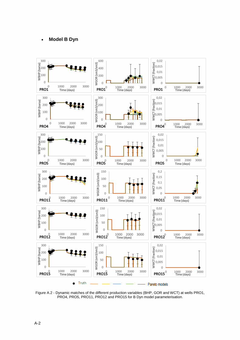
A-2
• Model B Dyn
Figure A.2 - Dynamic matches of the different production variables (BHP, GOR and WCT) at wells PRO1, PRO4, PRO5, PRO11, PRO12 and PRO15 for B Dyn model parameterisation.
0
100
200
300
0 1000 2000 3000
WB
HP
(bar
sa)
Time (days)PRO1
0
200
400
600
0 1000 2000 3000
WG
OR
(sm
3/sm
3)
Time (days)PRO1
0
0,005
0,01
0,015
0,02
0 1000 2000 3000
WW
CT
(fra
ctio
n)
Time (days)PRO1
0
100
200
300
0 1000 2000 3000
WB
HP
(bar
sa)
Time (days)PRO4
0
100
200
300
0 1000 2000 3000
WG
OR
(sm
3/sm
3)
Time (days)PRO4
0
0,005
0,01
0,015
0,02
0 1000 2000 3000
WW
CT
(fra
ctio
n)
Time (days)PRO4
0
100
200
300
0 1000 2000 3000
WB
HP
(bar
sa)
Time (days)PRO5
0
50
100
150
0 1000 2000 3000
WG
OR
(sm
3/sm
3)
Time (days)PRO5
0
0,005
0,01
0,015
0,02
0 1000 2000 3000
WW
CT
(fra
ctio
n)
Time (days)PRO5
0
100
200
300
0 1000 2000 3000
WB
HP
(bar
sa)
Time (days)PRO11
0
50
100
150
0 1000 2000 3000
WG
OR
(sm
3/sm
3)
Time (dyas)PRO11
0
0,05
0,1
0,15
0,2
0 1000 2000 3000
WW
CT
(fra
ctio
n)
Time (days)PRO11
0
100
200
300
0 1000 2000 3000
WB
HP
(bar
sa)
Time (days)PRO12
0
50
100
150
0 1000 2000 3000
WG
OR
(sm
3/sm
3)
Time (dyas)PRO12
0
0,005
0,01
0,015
0,02
0 1000 2000 3000
WW
CT
(fra
ctio
n)
Time (days)PRO12
0
100
200
300
0 1000 2000 3000
WB
HP
(bar
sa)
Time (days)PRO15
0
50
100
150
0 1000 2000 3000
WG
OR
(sm
3/sm
3)
Time (days)PRO15
0
0,005
0,01
0,015
0,02
0 1000 2000 3000
WW
CT
(fra
ctio
n)
Time (days)PRO15
A-3
• Model B Sta&Dyn
Figure A.3 - Dynamic matches of the different production variables (BHP, GOR and WCT) at wells PRO1, PRO4, PRO5, PRO11, PRO12 and PRO15 for B Sta&Dyn model parameterisation.
0
100
200
300
0 1000 2000 3000
WB
HP
(bar
sa)
Time (days)PRO1
0
200
400
600
0 1000 2000 3000WG
OR
(sm
3/sm
3)
Time (days)PRO1
0
0,005
0,01
0,015
0,02
0 1000 2000 3000
WW
CT
(fra
ctio
n)
Time (days)PRO1
0
100
200
300
0 1000 2000 3000
WB
HP
(bar
sa)
Time (days)PRO4
0
100
200
300
0 1000 2000 3000
WG
OR
(sm
3/sm
3)
Time (days)PRO4
0
0,005
0,01
0,015
0,02
0 1000 2000 3000
WW
CT
(fra
ctio
n)
Time (days)PRO4
0
100
200
300
0 1000 2000 3000
WB
HP
(bar
sa)
Time (days)PRO5
0
50
100
150
0 1000 2000 3000
WG
OR
(sm
3/sm
3)
Time (days)PRO5
0
0,2
0,4
0,6
0,8
0 1000 2000 3000W
WC
T (f
ract
ion
)Time (days)PRO5
0
100
200
300
0 1000 2000 3000
WB
HP
(bar
sa)
Time (days)PRO11
0
50
100
150
0 1000 2000 3000WG
OR
(sm
3/sm
3)
Time (dyas)PRO11
0
0,1
0,2
0,3
0 1000 2000 3000
WW
CT
(fra
ctio
n)
Time (days)PRO11
0
100
200
300
0 1000 2000 3000
WB
HP
(bar
sa)
Time (days)PRO12
0
50
100
150
0 1000 2000 3000
WG
OR
(sm
3/sm
3)
Time (dyas)PRO12
0
0,01
0,02
0,03
0 1000 2000 3000
WW
CT
(fra
ctio
n)
Time (days)PRO12
0
100
200
300
0 1000 2000 3000
WB
HP
(bar
sa)
Time (days)PRO15
0
50
100
150
0 1000 2000 3000
WG
OR
(sm
3/sm
3)
Time (days)PRO15
0
0,005
0,01
0,015
0,02
0 1000 2000 3000
WW
CT
(fra
ctio
n)
Time (days)PRO15
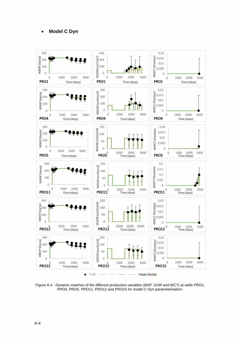
A-4
• Model C Dyn
Figure A.4 - Dynamic matches of the different production variables (BHP, GOR and WCT) at wells PRO1, PRO4, PRO5, PRO11, PRO12 and PRO15 for model C Dyn parameterisation.
0
100
200
300
0 1000 2000 3000
WB
HP
(bar
sa)
Time (days)PRO1
0
200
400
600
0 1000 2000 3000WG
OR
(sm
3/s
m3)
Time (dyas)PRO1
0
0,005
0,01
0,015
0,02
0 1000 2000 3000WW
CT
(fra
ctio
n)
Time (days)PRO1
0
100
200
300
0 1000 2000 3000
WB
HP
(bar
sa)
Time (days)PRO4
0
100
200
300
0 1000 2000 3000WG
OR
(sm
3/sm
3)
Time (days)PRO4
0
0,005
0,01
0,015
0,02
0 1000 2000 3000
WW
CT
(fra
ctio
n)
Time (days)PRO4
0
100
200
300
0 1000 2000 3000
WB
HP
(bar
sa)
Time (days)PRO5
0
50
100
150
0 1000 2000 3000
WG
OR
(sm
3/sm
3)
Time (days)PRO5
0
0,005
0,01
0,015
0,02
0 1000 2000 3000W
WC
T (f
ract
ion
)Time (days)PRO5
0
100
200
300
0 1000 2000 3000
WB
HP
(bar
sa)
Time (days)PRO11
0
50
100
150
0 1000 2000 3000
WG
OR
(sm
3/sm
3)
Time (dyas)PRO11
0
0,05
0,1
0,15
0,2
0 1000 2000 3000
WW
CT
(fra
ctio
n)
Time (days)PRO11
0
100
200
300
0 1000 2000 3000
WB
HP
(bar
sa)
Time (days)PRO12
0
50
100
150
0 1000 2000 3000
WG
OR
(sm
3/sm
3)
Time (dyas)PRO12
0
0,005
0,01
0,015
0,02
0 1000 2000 3000
WW
CT
(fra
ctio
n)
Time (days)PRO12
0
100
200
300
0 1000 2000 3000
WB
HP
(bar
sa)
Time (days)PRO15
0
50
100
150
0 1000 2000 3000
WG
OR
(sm
3/sm
3)
Time (days)PRO15
0
0,005
0,01
0,015
0,02
0 1000 2000 3000
WW
CT
(fra
ctio
n)
Time (days)PRO15
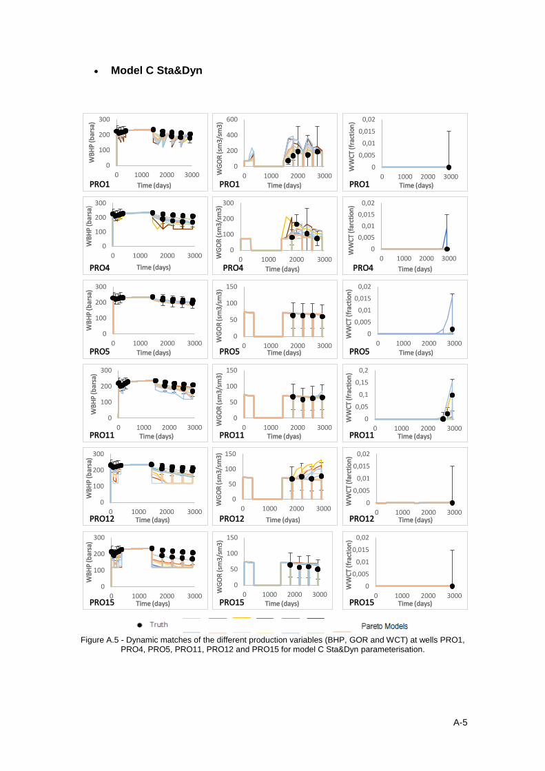
A-5
• Model C Sta&Dyn
Figure A.5 - Dynamic matches of the different production variables (BHP, GOR and WCT) at wells PRO1,
PRO4, PRO5, PRO11, PRO12 and PRO15 for model C Sta&Dyn parameterisation.
0
100
200
300
0 1000 2000 3000
WB
HP
(bar
sa)
Time (days)PRO1
0
200
400
600
0 1000 2000 3000WG
OR
(sm
3/sm
3)
Time (days)PRO1
0
0,005
0,01
0,015
0,02
0 1000 2000 3000
WW
CT
(fra
ctio
n)
Time (days)PRO1
0
100
200
300
0 1000 2000 3000
WB
HP
(bar
sa)
Time (days)PRO4
0
100
200
300
0 1000 2000 3000WG
OR
(sm
3/sm
3)
Time (days)PRO4
0
0,005
0,01
0,015
0,02
0 1000 2000 3000
WW
CT
(far
ctio
n)
Time (days)PRO4
0
100
200
300
0 1000 2000 3000
WB
HP
(bar
sa)
Time (days)PRO5
0
50
100
150
0 1000 2000 3000
WG
OR
(sm
3/sm
3)
Time (days)PRO5
0
0,005
0,01
0,015
0,02
0 1000 2000 3000W
WC
T (f
ract
ion
)Time (days)PRO5
0
100
200
300
0 1000 2000 3000
WB
HP
(bar
sa)
Time (days)PRO11
0
50
100
150
0 1000 2000 3000WG
OR
(sm
3/sm
3)
Time (dyas)PRO11
0
0,05
0,1
0,15
0,2
0 1000 2000 3000
WW
CT
(fra
ctio
n)
Time (days)PRO11
0
100
200
300
0 1000 2000 3000
WB
HP
(bar
sa)
Time (days)PRO12
0
50
100
150
0 1000 2000 3000
WG
OR
(sm
3/sm
3)
Time (dyas)PRO12
0
0,005
0,01
0,015
0,02
0 1000 2000 3000
WW
CT
(far
ctio
n)
Time (days)PRO12
0
100
200
300
0 1000 2000 3000
WB
HP
(bar
sa)
Time (days)PRO15
0
50
100
150
0 1000 2000 3000WG
OR
(sm
3/sm
3)
Time (days)PRO15
0
0,005
0,01
0,015
0,02
0 1000 2000 3000
WW
CT
(fra
ctio
n)
Time (days)PRO15

A-6
This page intentionally left blank

B-1
Appendix B – Forecasting and Uncertainty Characterization
• Model A
Figure B.1 - Forecasting of the different production variables (BHP, GOR and WCT) at wells PRO1, PRO4, PRO5, PRO11, PRO12 and PRO15 for model A parameterisation.
0
100
200
0 2000 4000 6000
WB
HP
(bar
sa)
Time (days)PRO1
0
100
200
0 2000 4000 6000W
GO
R (s
m3/
sm3)
Time (days)PRO1
0
0,2
0,4
0,6
0 2000 4000 6000
WW
CT
(fra
ctio
n)
Time (days)PRO1
0
100
200
0 2000 4000 6000
WB
HP
(bar
sa)
Time (days)PRO4
0
50
100
150
0 2000 4000 6000
WG
OR
(sm
3/sm
3)
Time (days)PRO4
0
0,2
0,4
0,6
0,8
0 2000 4000 6000
WW
CT
(fra
ctio
n)
Time (days)PRO4
0
100
200
0 2000 4000 6000
WB
HP
(bar
sa)
Time (days)PRO5
0
20
40
60
80
0 2000 4000 6000WG
OR
(sm
3/sm
3)
Time (days)PRO5
0
0,2
0,4
0 2000 4000 6000
WW
CT
(fra
ctio
n)
Time (days)PRO5
0
100
200
0 2000 4000 6000
WB
HP
(bar
sa)
Time (days)PRO11
0
50
100
150
200
0 2000 4000 6000
WG
OR
(sm
3/sm
3)
Time (days)PRO11
0
0,2
0,4
0,6
0 2000 4000 6000
WW
CT
(fra
ctio
n)
Time (days)PRO11
0
100
200
300
400
0 2000 4000 6000
WB
HP
(bar
sa)
Time (days)PRO12
0
20
40
60
80
0 2000 4000 6000WG
OR
(sm
3/sm
3)
Time (days)PRO12
0
0,2
0,4
0 2000 4000 6000
WW
CT
(fra
ctio
n)
Time (days)PRO12
0
100
200
0 2000 4000 6000
WB
HP
(bar
sa)
Time (days)PRO15
0
50
100
150
200
0 2000 4000 6000WG
OR
(sm
3/sm
3)
Time (days)PRO15
0
0,05
0,1
0 2000 4000 6000
WW
CT
(fra
ctio
n)
Time (days)PRO15

B-2
• Model B Dyn
Figure B.2 - Forecasting of the different production variables (BHP, GOR and WCT) at wells PRO1, PRO4, PRO5, PRO11, PRO12 and PRO15 for model B Dyn parameterisation.
0
100
200
0 2000 4000 6000
WB
HP
(bar
sa)
Time (days)PRO1
0
100
200
0 2000 4000 6000
WG
OR
(sm
3/sm
3)
Time (days)PRO1
0
0,0001
0,0002
0 2000 4000 6000
WW
CT
(fra
ctio
n)
Time (days)PRO1
0
100
200
0 2000 4000 6000
WB
HP
(bar
sa)
Time (days)PRO4
0
50
100
150
0 2000 4000 6000WG
OR
(sm
3/sm
3)
Time (days)PRO4
0
0,2
0,4
0,6
0,8
0 2000 4000 6000
WW
CT
(fra
ctio
n)
Time (days)PRO4
0
100
200
0 2000 4000 6000
WB
HP
(bar
sa)
Time (days)PRO5
0
20
40
60
80
0 2000 4000 6000WG
OR
(sm
3/sm
3)
Time (days)PRO5
0
0,05
0,1
0 2000 4000 6000W
WC
T (f
ract
ion
)Time (days)PRO5
0
100
200
0 2000 4000 6000
WB
HP
(bar
sa)
Time (days)PRO11
0
50
100
150
200
0 2000 4000 6000
WG
OR
(sm
3/sm
3)
Time (days)PRO11
0
0,2
0,4
0,6
0 2000 4000 6000
WW
CT
(fra
ctio
n)
Time (days)PRO11
0
100
200
300
400
0 2000 4000 6000
WB
HP
(bar
sa)
Time (days)PRO12
0
20
40
60
80
0 2000 4000 6000
WG
OR
(sm
3/sm
3)
Time (days)PRO12
0
0,2
0,4
0 2000 4000 6000
WW
CT
(fra
ctio
n)
Time (days)PRO12
0
100
200
0 2000 4000 6000
WB
HP
(bar
sa)
Time (days)PRO15
0
50
100
150
200
0 2000 4000 6000
WG
OR
(sm
3/sm
3)
Time (days)PRO15
0
0,0005
0,001
0 2000 4000 6000
WW
CT
(fra
ctio
n)
Time (days)PRO15
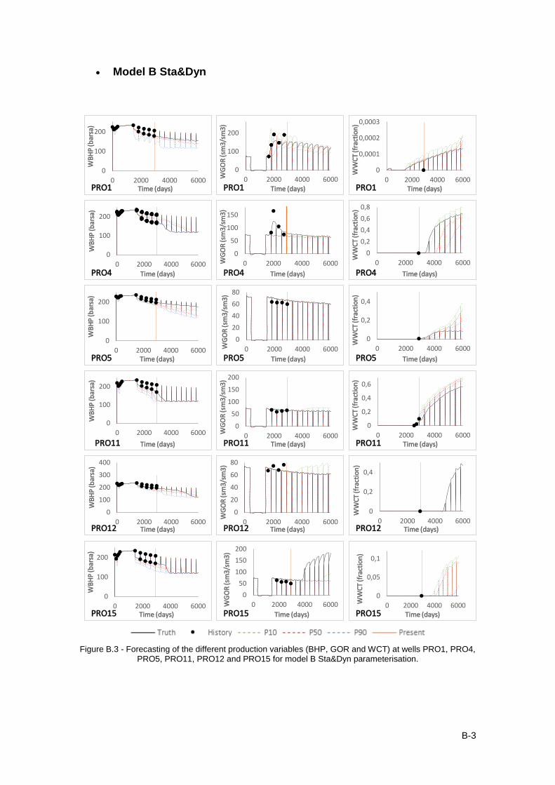
B-3
• Model B Sta&Dyn
Figure B.3 - Forecasting of the different production variables (BHP, GOR and WCT) at wells PRO1, PRO4, PRO5, PRO11, PRO12 and PRO15 for model B Sta&Dyn parameterisation.
0
100
200
0 2000 4000 6000
WB
HP
(bar
sa)
Time (days)PRO1
0
100
200
0 2000 4000 6000WG
OR
(sm
3/sm
3)
Time (days)PRO1
0
0,0001
0,0002
0,0003
0 2000 4000 6000
WW
CT
(fra
ctio
n)
Time (days)PRO1
0
100
200
0 2000 4000 6000
WB
HP
(bar
sa)
Time (days)PRO4
0
50
100
150
0 2000 4000 6000WG
OR
(sm
3/sm
3)
Time (days)PRO4
0
0,2
0,4
0,6
0,8
0 2000 4000 6000
WW
CT
(fra
ctio
n)
Time (days)PRO4
0
100
200
0 2000 4000 6000
WB
HP
(bar
sa)
Time (days)PRO5
0
20
40
60
80
0 2000 4000 6000WG
OR
(sm
3/sm
3)
Time (days)PRO5
0
0,2
0,4
0 2000 4000 6000W
WC
T (f
ract
ion
)Time (days)PRO5
0
100
200
0 2000 4000 6000
WB
HP
(bar
sa)
Time (days)PRO11
0
50
100
150
200
0 2000 4000 6000
WG
OR
(sm
3/sm
3)
Time (days)PRO11
0
0,2
0,4
0,6
0 2000 4000 6000
WW
CT
(fra
ctio
n)
Time (days)PRO11
0
100
200
300
400
0 2000 4000 6000
WB
HP
(bar
sa)
Time (days)PRO12
0
20
40
60
80
0 2000 4000 6000
WG
OR
(sm
3/sm
3)
Time (days)PRO12
0
0,2
0,4
0 2000 4000 6000
WW
CT
(fra
ctio
n)
Time (days)PRO12
0
100
200
0 2000 4000 6000
WB
HP
(bar
sa)
Time (days)PRO15
0
50
100
150
200
0 2000 4000 6000WG
OR
(sm
3/sm
3)
Time (days)PRO15
0
0,05
0,1
0 2000 4000 6000WW
CT
(fra
ctio
n)
Time (days)PRO15
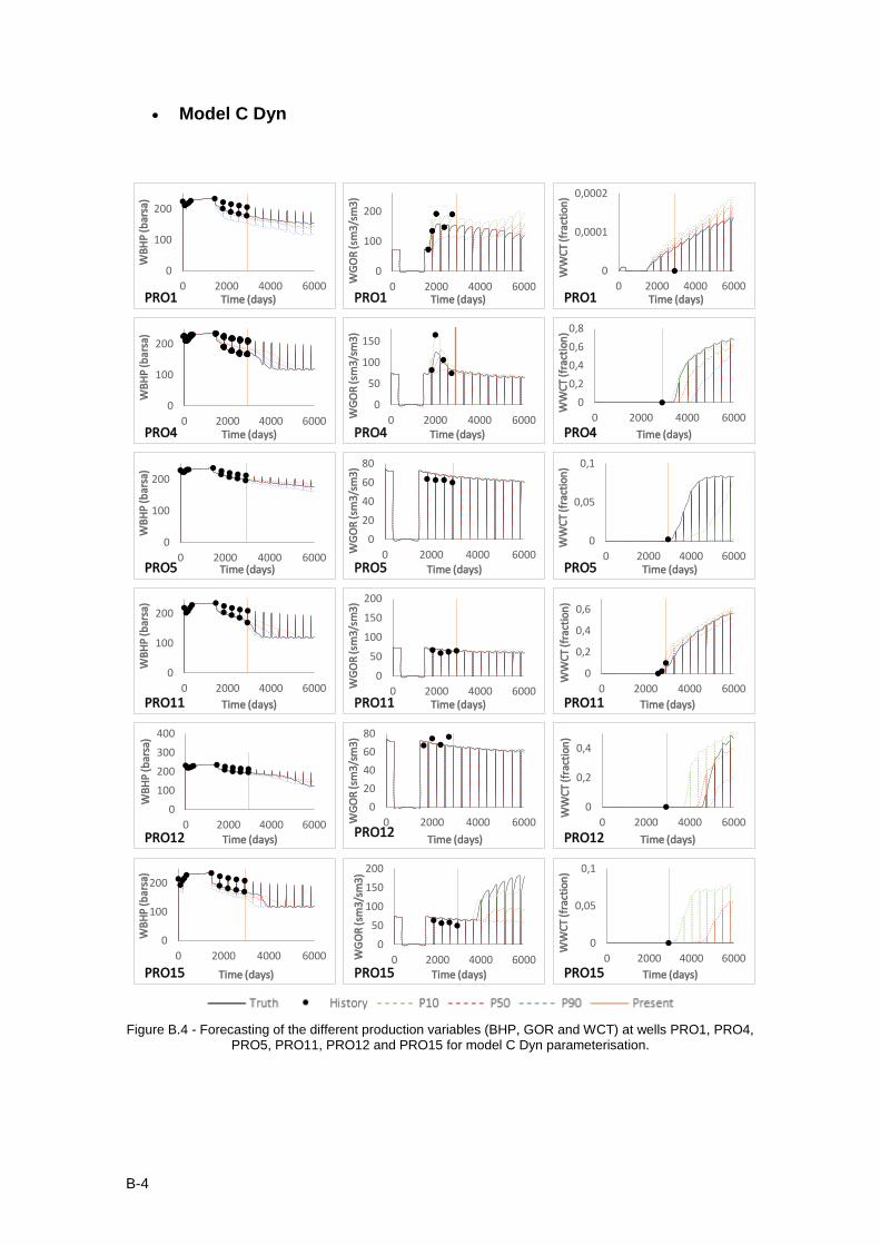
B-4
• Model C Dyn
Figure B.4 - Forecasting of the different production variables (BHP, GOR and WCT) at wells PRO1, PRO4, PRO5, PRO11, PRO12 and PRO15 for model C Dyn parameterisation.
0
100
200
0 2000 4000 6000
WB
HP
(bar
sa)
Time (days)PRO1
0
100
200
0 2000 4000 6000
WG
OR
(sm
3/sm
3)
Time (days)PRO1
0
0,0001
0,0002
0 2000 4000 6000
WW
CT
(fra
ctio
n)
Time (days)PRO1
0
100
200
0 2000 4000 6000
WB
HP
(bar
sa)
Time (days)PRO4
0
50
100
150
0 2000 4000 6000WG
OR
(sm
3/sm
3)
Time (days)PRO4
0
0,2
0,4
0,6
0,8
0 2000 4000 6000
WW
CT
(fra
ctio
n)
Time (days)PRO4
0
100
200
0 2000 4000 6000
WB
HP
(bar
sa)
Time (days)PRO5
0
20
40
60
80
0 2000 4000 6000WG
OR
(sm
3/sm
3)
Time (days)PRO5
0
0,05
0,1
0 2000 4000 6000W
WC
T (f
ract
ion
)Time (days)PRO5
0
100
200
0 2000 4000 6000
WB
HP
(bar
sa)
Time (days)PRO11
0
50
100
150
200
0 2000 4000 6000
WG
OR
(sm
3/sm
3)
Time (days)PRO11
0
0,2
0,4
0,6
0 2000 4000 6000
WW
CT
(fra
ctio
n)
Time (days)PRO11
0
100
200
300
400
0 2000 4000 6000
WB
HP
(bar
sa)
Time (days)PRO12
0
20
40
60
80
0 2000 4000 6000WG
OR
(sm
3/sm
3)
Time (days)PRO12
0
0,2
0,4
0 2000 4000 6000
WW
CT
(fra
ctio
n)
Time (days)PRO12
0
100
200
0 2000 4000 6000
WB
HP
(bar
sa)
Time (days)PRO15
0
50
100
150
200
0 2000 4000 6000WG
OR
(sm
3/sm
3)
Time (days)PRO15
0
0,05
0,1
0 2000 4000 6000
WW
CT
(fra
ctio
n)
Time (days)PRO15
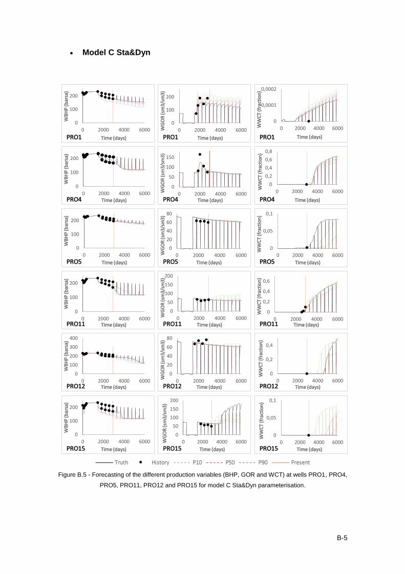
B-5
• Model C Sta&Dyn
Figure B.5 - Forecasting of the different production variables (BHP, GOR and WCT) at wells PRO1, PRO4,
PRO5, PRO11, PRO12 and PRO15 for model C Sta&Dyn parameterisation.
0
100
200
0 2000 4000 6000
WB
HP
(bar
sa)
Time (days)PRO1
0
100
200
0 2000 4000 6000WG
OR
(sm
3/sm
3)
Time (days)PRO1
0
0,0001
0,0002
0 2000 4000 6000WW
CT
(fra
ctio
n)
Time (days)PRO1
0
100
200
0 2000 4000 6000
WB
HP
(bar
sa)
Time (days)PRO4
0
50
100
150
0 2000 4000 6000WG
OR
(sm
3/sm
3)
Time (days)PRO4
0
0,2
0,4
0,6
0,8
0 2000 4000 6000
WW
CT
(fra
ctio
n)
Time (days)PRO4
0
100
200
0 2000 4000 6000
WB
HP
(bar
sa)
Time (days)PRO5
0
20
40
60
80
0 2000 4000 6000WG
OR
(sm
3/sm
3)
Time (days)PRO5
0
0,05
0,1
0 2000 4000 6000W
WC
T (f
ract
ion
)Time (days)PRO5
0
100
200
0 2000 4000 6000
WB
HP
(bar
sa)
Time (days)PRO11
0
50
100
150
200
0 2000 4000 6000WG
OR
(sm
3/sm
3)
Time (days)PRO11
0
0,2
0,4
0,6
0 2000 4000 6000
WW
CT
(fra
ctio
n)
Time (days)PRO11
0
100
200
300
400
0 2000 4000 6000
WB
HP
(bar
sa)
Time (days)PRO12
0
20
40
60
80
0 2000 4000 6000
WG
OR
(sm
3/sm
3)
Time (days)PRO12
0
0,2
0,4
0 2000 4000 6000
WW
CT
(fra
ctio
n)
Time (days)PRO12
0
100
200
0 2000 4000 6000
WB
HP
(bar
sa)
Time (days)PRO15
0
50
100
150
200
0 2000 4000 6000WG
OR
(sm
3/sm
3)
Time (days)PRO15
0
0,05
0,1
0 2000 4000 6000
WW
CT
(fra
ctio
n)
Time (days)PRO15

B-6
• BMA based in Dynamic Likelihood
Figure B.6 - Forecasting of the different production variables (BHP, GOR and WCT) at wells PRO1, PRO4, PRO5, PRO11, PRO12 and PRO15 for the BMA based in dynamic likelihood.
0
100
200
0 2000 4000 6000
WB
HP
(bar
sa)
Time (days)PRO1
0
100
200
0 2000 4000 6000
WG
OR
(sm
3/sm
3)
Time (days)PRO1
0
0,0001
0,0002
0 2000 4000 6000
WW
CT
(fra
ctio
n)
Time (days)PRO1
0
100
200
0 2000 4000 6000
WB
HP
(bar
sa)
Time (days)PRO4
0
50
100
150
0 2000 4000 6000
WG
OR
(sm
3/sm
3)
Time (days)PRO4
0
0,2
0,4
0,6
0,8
0 2000 4000 6000
WW
CT
(fra
ctio
n)
Time (days)PRO4
0
100
200
0 2000 4000 6000
WB
HP
(bar
sa)
Time (days)PRO5
0
20
40
60
80
0 2000 4000 6000
WG
OR
(sm
3/sm
3)
Time (days)PRO5
0
0,2
0,4
0 2000 4000 6000W
WC
T (f
ract
ion
)Time (days)PRO5
0
100
200
0 2000 4000 6000
WB
HP
(bar
sa)
Time (days)PRO11
0
50
100
0 2000 4000 6000WG
OR
(sm
3/sm
3)
Time (days)PRO11
0
0,2
0,4
0,6
0 2000 4000 6000
WW
CT
(fra
ctio
n)
Time (days)PRO11
0
100
200
300
400
0 2000 4000 6000
WB
HP
(bar
sa)
Time (days)PRO12
0
20
40
60
80
0 2000 4000 6000
WG
OR
(sm
3/sm
3)
Time (days)PRO12
0
0,2
0,4
0 2000 4000 6000
WW
CT
(fra
ctio
n)
Time (days)PRO12
0
100
200
0 2000 4000 6000
WB
HP
(bar
sa)
Time (days)PRO15
0
50
100
150
200
0 2000 4000 6000WG
OR
(sm
3/sm
3)
Time (days)PRO15
0
0,05
0,1
0 2000 4000 6000
WW
CT
(fra
ctio
n)
Time (days)PRO15
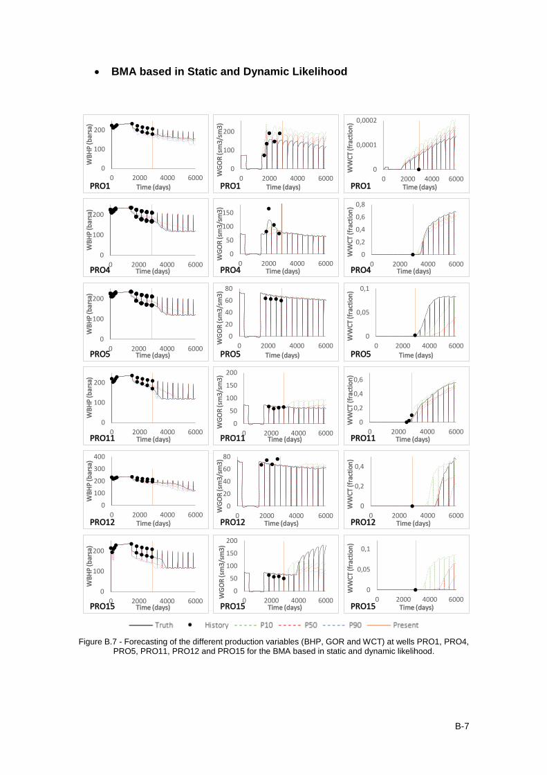
B-7
• BMA based in Static and Dynamic Likelihood
Figure B.7 - Forecasting of the different production variables (BHP, GOR and WCT) at wells PRO1, PRO4, PRO5, PRO11, PRO12 and PRO15 for the BMA based in static and dynamic likelihood.
0
100
200
0 2000 4000 6000
WB
HP
(bar
sa)
Time (days)PRO1
0
100
200
0 2000 4000 6000
WG
OR
(sm
3/sm
3)
Time (days)PRO1
0
0,0001
0,0002
0 2000 4000 6000
WW
CT
(fra
ctio
n)
Time (days)PRO1
0
100
200
0 2000 4000 6000
WB
HP
(bar
sa)
Time (days)PRO4
0
50
100
150
0 2000 4000 6000
WG
OR
(sm
3/sm
3)
Time (days)PRO4
0
0,2
0,4
0,6
0,8
0 2000 4000 6000
WW
CT
(fra
ctio
n)
Time (days)PRO4
0
100
200
0 2000 4000 6000
WB
HP
(bar
sa)
Time (days)PRO5
0
20
40
60
80
0 2000 4000 6000WG
OR
(sm
3/sm
3)
Time (days)PRO5
0
0,05
0,1
0 2000 4000 6000W
WC
T (f
ract
ion
)Time (days)PRO5
0
100
200
0 2000 4000 6000
WB
HP
(bar
sa)
Time (days)PRO11
0
50
100
150
200
0 2000 4000 6000
WG
OR
(sm
3/sm
3)
Time (days)PRO11
0
0,2
0,4
0,6
0 2000 4000 6000
WW
CT
(fra
ctio
n)
Time (days)PRO11
0
100
200
300
400
0 2000 4000 6000
WB
HP
(bar
sa)
Time (days)PRO12
0
20
40
60
80
0 2000 4000 6000
WG
OR
(sm
3/sm
3)
Time (days)PRO12
0
0,2
0,4
0 2000 4000 6000
WW
CT
(fra
ctio
n)
Time (days)PRO12
0
100
200
0 2000 4000 6000
WB
HP
(bar
sa)
Time (days)PRO15
0
50
100
150
200
0 2000 4000 6000
WG
OR
(sm
3/sm
3)
Time (days)PRO15
0
0,05
0,1
0 2000 4000 6000
WW
CT
(fra
ctio
n)
Time (days)PRO15