balancing of wheel suspension packaging, …...master’s thesis in product development balancing of...
TRANSCRIPT

Department of Product and Production Development
Division of Product Development
CHALMERS UNIVERSITY OF TECHNOLOGY
Gothenburg, Sweden 2016
Balancing of Wheel Suspension Packaging, Performance and Weight Master’s Thesis in Product Development
KANISHK BHADANI
JOAKIM SKÖN

MASTER’S THESIS IN PRODUCT DEVELOPMENT
Balancing of Wheel Suspension Packaging,
Performance and Weight
KANISHK BHADANI
JOAKIM SKÖN
Department of Product and Production Development
Division of Product development
CHALMERS UNIVERSITY OF TECHNOLOGY
Göteborg, Sweden 2016

Balancing of Wheel Suspension Packaging, Performance and Weight
KANISHK BHADANI
JOAKIM SKÖN
© KANISHK BHADANI & JOAKIM SKÖN, 2016-06-20
Supervisor: Harald Hasselblad, Volvo Car Corporation
Supervisor: Dr. Magnus Bengtsson, Department of Product and Production
Development
Examiner: Dr. Magnus Bengtsson, Department of Product and Production
Development
Master’s Thesis 2016
Department of Product and Production Development
Division of Product development
Chalmers University of Technology
SE-412 96 Göteborg
Telephone: + 46 (0)31-772 1000
Cover: SPA Rear Wheel Suspension. Chalmers Reproservice Gothenburg, Sweden 2016

CHALMERS, Product Development, Master’s Thesis 2016 i
Balancing of Wheel Suspension Packaging, Performance and Weight
Master’s thesis in Product Development
KANISHK BHADANI
JOAKIM SKÖN
Department of Product and Production Development
Division of Product development
Chalmers University of Technology
Abstract
In today’s automotive industry there is a growing demand for more fuel efficient
vehicles and reduced development times. These trends are driven by stricter
environmental regulations, a growing environmental awareness, and increasing
technology development which pushes the vehicle manufacturers to produce lighter
vehicles in shorter time to stay competitive.
The aim with this master thesis is to find a process and tools to balance packaging conflicts. Finding an optimized and balanced components that fulfils the requirements
in an early phase of the product development is a prerequisite for enabling more
competitive lead times, costs, weights and minimizing the risk for late design changes.
A complex system, such as a wheel suspension, requires a process that enables CAE
driven development where a natural part is optimization and a tight coupling between
design and verification engineers. Today, the development of the wheel suspension is
carried out by developing concepts based on engineering experience which are then
verified against predefined requirements. If the concepts do not fulfill the requirements
they are iteratively updated and re-verified. This process lack collaboration which lead
to increased number of iterations and more resource consumption before a feasible
design is obtained.
This thesis work has been an initiation of CAE driven development and design volume
optimization at the Wheel Suspension department at Volvo Cars. The thesis work
consisted of two parts, where the first part was to develop a workflow process for the
wheel suspension development where optimization is an integrated part of the process.
The second part was a technical working process of how to balance packaging conflicts
through performing shape and topology optimization on multiple components
simultaneously, to obtain system level optimization.
Key words: Optimization, Design Volume Optimization, Process Development, Shape
Optimization, Topology Optimization, CAE Driven Development.

ii CHALMERS, Product Development, Master’s Thesis 2016

CHALMERS, Product Development, Master’s Thesis 2016 iii
Acknowledgements
We would like to thank Harald Hasselblad, our supervisor at Volvo Car Corporation,
for his guidance and encouragements throughout the thesis.
We would like to thank Magnus Bengtsson, our supervisor and examiner at Chalmers
University of Technology, for his guidance and assistance during the thesis.
We would like to express our gratitude to Daniel Molin, Iris Blume and Per
Björklund, Volvo Car Corporation, for providing valuable knowledge through
discussions and feedback.
Further we would like to thank Britta Käck and Joakim Truedsson, Altair Engineering
Inc., for supporting us with software related issues during the thesis.
Lastly we would like to thank the members of the Master Thesis projects in the
Optimization Culture Arena for valuable knowledge and collaboration throughout the
thesis.
Göteborg 2016-06-20
KANISHK BHADANI
JOAKIM SKÖN

iv CHALMERS, Product Development, Master’s Thesis 2016

CHALMERS, Product Development, Master’s Thesis 2016 v
Table of Contents
Abstract ....................................................................................................................... i
Acknowledgements .................................................................................................. iii
Notations ..................................................................................................................vii
1 Introduction ............................................................................................................ 1
1.1 Volvo Car Corporation .................................................................................... 1
1.2 Background ..................................................................................................... 1
1.3 Aim and Purpose ............................................................................................. 2
1.4 Description of Design Volume Conflict .......................................................... 2
1.5 Limitations ...................................................................................................... 3
1.6 Research Questions ......................................................................................... 3
1.7 Thesis Setup .................................................................................................... 3
2 Literature Study ..................................................................................................... 5
2.1 Background of the Wheel Suspension ............................................................ 5
2.2 Introduction to Design Optimization............................................................... 5
2.3 Topology Optimization ................................................................................... 7
2.4 Practical Approaches to Topology Optimization ............................................ 8
2.5 Design-space and Influence on Topology ....................................................... 9
2.6 Information Sharing in the Optimization Process ......................................... 10
3 Method ................................................................................................................. 11
3.1 Development Process for Wheel Suspension Components ........................... 11
3.2 Design Volume Optimization Process .......................................................... 12
4 Pilot Study ............................................................................................................ 15
4.1 Current Process Investigation ........................................................................ 15
4.2 Analysis of the Current Development Process .............................................. 17
5 Proposed Development Process ........................................................................... 19
5.1 Proposed Development Process .................................................................... 19
5.2 Challenges for the New Development Process ............................................. 21
6 Tests on Sample Components .............................................................................. 23
6.1 Simplified Model Setup ................................................................................ 23
6.2 Shape and Topology Optimization ................................................................ 27
6.3 Combined Model Optimization ..................................................................... 29
6.4 Control Setting Test for Shape and Topology Optimization......................... 32
7 Design Volume Optimization Process ................................................................. 37

vi CHALMERS, Product Development, Master’s Thesis 2016
7.1 Design Volume Optimization ........................................................................ 37
7.2 Sub-functions for Deign Volume Optimization ............................................ 38
7.3 FE Modeling .................................................................................................. 40
7.4 Topology Optimization ................................................................................. 41
7.5 Shape and Topology Optimization ................................................................ 43
7.6 Combined Optimization ................................................................................ 44
8 Verification of the Design Volume Optimization Process .................................. 47
8.1 Execution of the Design Volume Optimization ............................................ 47
8.2 Evaluation of the Design Volume Optimization ........................................... 58
9 Discussion and Future Work ................................................................................ 61
9.1 Proposed Wheel Suspension Development Process ...................................... 61
9.2 Design Volume Optimization Process .......................................................... 62
9.3 Optimization Cluster ..................................................................................... 63
9.4 Future Work .................................................................................................. 63
10 Conclusion ........................................................................................................... 65
11 References ............................................................................................................ 67
Appendix 1 Data Collection Process ............................................................................. I
Appendix 2 Geometry Guidelines ................................................................................ II
Appendix 3 Mesh Guidelines ........................................................................................ V
Appendix 4 Boundary Conditions and Loading Guidelines ..................................... VIII
Appendix 5 Topology and Shape Optimization Guideline ..........................................IX
Appendix 6 Morphing Guideline .................................................................................XI
Appendix 7 Post Processing Guidelines ................................................................... XIII

CHALMERS, Product Development, Master’s Thesis 2016 vii
Notations
ρ Density
ADAMS Software for Kinematic and Dynamic simulations
CAD Computer Aided Design
CAE Computer Aided Engineering
Catia V5 Software for Computer Aided Design
ESO Evolutionary Structural Optimization
FE Finite Element
FEA Finite Element Analysis
FEM Finite Element Model
IDEF0 ICAM Definition for Function Modeling
Ḵ Penalized Stiffness K Real Stiffness
LCA Lower Control Arm
MFD Method of Feasible Directions
OFAT One factor at a time
P Penalization factor
SBCD Simulation Based Concept Design
SIMP Simple Isotropic Material with Penalization
SQP Sequential Quadratic Programming
TR Technical Regulations
UCA Upper Control Arm
VD Vehicle Dynamics

viii CHALMERS, Product Development, Master’s Thesis 2016
CHALMERS, Product Development, Master’s Thesis 2016 1
1 Introduction This master thesis has been carried out at Volvo Car Corporation (Volvo Cars) to
develop a process for optimizing and balancing packaging of adjacent components of
the wheel suspension. This chapter begins with an introduction to Volvo Cars, followed
by background, aim and purpose, description of the design volume conflict, limitations,
research questions, and thesis setup of the thesis work.
1.1 Volvo Car Corporation
Volvo Cars is a car manufacturer that was founded in Sweden in 1927 with headquarter
in Gothenburg, Sweden. Volvo Cars is a global company with approximately 28,500
employees worldwide. Volvo cars is presently owned by Zhejiang Geely Holding
(Geely Holding) of China and has production in Sweden, Belgium, China and Malaysia.
Volvo Cars’ development, design and marketing are carried out at the Torslanda,
Gothenburg site. Volvo Cars produces cars for the premium segment that includes
sedans, wagons, sports wagons, cross country cars and SUVs. In 2015 a total of 503,127
cars was sold in about 100 countries with an operating income of 6,620 MSEK.
1.2 Background
In today’s automotive industry there is a growing demand for more fuel efficient
vehicles and reduced development times. These trends are driven by stricter
environmental regulations, a growing environmental awareness, and increasing
technology development which pushes the vehicle manufacturers to produce lighter
vehicles in shorter time to stay competitive.
Finding an optimized and balanced components that fulfils the requirements in an early
phase of the product development is a prerequisite for enabling more competitive lead
times, costs, weights and minimizing the risk for late design changes. A complex
system, such as a wheel suspension, requires a process that enables CAE driven
development where a natural part is optimization and a tight coupling between design
and verification (CAD & CAE). Today, the development of the wheel suspension is
carried out by developing concepts based on engineering experience which are then
verified against predefined requirements. If the concepts do not fulfill the requirements
they are iteratively updated and re-verified. This process lack collaboration which lead
to increased number of iterations and more resource consumption before a feasible
design is obtained. Therefore, there is a need to develop a process to collaborate the
work of different departments, in order to save time, resources, and improve
performance.
The use of structural optimization in industry through commercial software has
increased during the past decade. It has shown great potential in generating concepts
for early stage development and can be used to solve a variety of problems. However,
the use of this method is limited in the current wheel suspension development process
at Volvo Cars.

2 CHALMERS, Product Development, Master’s Thesis 2016
1.3 Aim and Purpose
The aim with this thesis work is to find a process to be implemented in the development
of wheel suspension components to optimize and balance packaging volumes of
adjacent components. The purpose of developing the process is to find the optimal
weight and performance for the rear wheel suspension. This requires an investigation
of how balancing of design volumes for conflicting components can be performed using
structural optimization. Finding a balanced solution regarding structural efficiency
between two adjacent systems or components enables a cost and weight efficient
solution.
1.4 Description of Design Volume Conflict
The components in the wheel suspension are currently designed within limited design
volumes which are defined early in the development process. The performance of each
component is dependent on the volume it is allowed to occupy and in order to improve
the performance, the design volume needs to be changed and balanced. Design volume
changes of the components in the wheel suspension are however in many cases
constrained by adjacent components’ design volumes which creates a conflict. By
balancing the design volumes of the two components in conflict, the system level
performance will be improved.
In this thesis work, the performance conflict between the Upper Control Arm (UCA)
and Lower Control Arm (LCA) from the S90/V90 configuration is investigated, see
Figure 1. The UCA is constrained both by the LCA and a body beam which limits its
performance, and by balancing the design volumes of these components the
performance of the wheel suspension can be increased.
Figure 1 - Illustration of the conflict between the UCA and LCA
UCA
LCA
Body Beam

CHALMERS, Product Development, Master’s Thesis 2016 3
1.5 Limitations
The thesis work is limited to the rear wheel suspension of the S90/V90
configuration in the SPA-platform.
The thesis work is limited to the interaction of two components, the UCA and
LCA of the wheel suspension.
Simplified load cases will be used at component level for performing linear
analysis.
The optimization setup will only consider weight minimization with respect to
stiffness requirements at component level.
The software package used to carry out the optimizations is HyperWorks 14.0.
The theory and mathematics behind different optimization methods will not be
investigated in any greater detail.
The thesis work is carried out by two students within a time frame of 20
weeks.
1.6 Research Questions
How to integrate CAD and CAE engineers work in order to implement
optimization in the early stages of wheel suspension development at Volvo
Cars?
How to perform simultaneous design volume optimization on two components
of the wheel suspension, which are competing for packaging volume?
1.7 Thesis Setup
This thesis work was carried out at the Weight Management and optimization
department (91770) in collaboration with the Rear Wheel suspension (94530) and the
Durability (91500) departments.
This thesis was a part of the Optimization Culture Arena at Volvo Cars which aims to
develop a cross technical knowledge network for common optimization competence
development. The thesis was also a part of a cluster of theses related to optimizing the
wheel suspension which aimed at sharing knowledge, information, and discuss
common challenges. The cluster consisted of three theses focusing on three different
segments of the wheel suspension development. The first was ”Optimization of Wheel
Suspension Packaging” followed by ”Balancing of Wheel Suspension Packaging,
Performance and Weight” and ”Structural Topology and Shape Optimization”. The
thesis ”Optimization of Wheel Suspension Packaging” was aimed at finding a suitable
methodology for efficient data transfer from CAE to CAD software, which reduces lead
time and increases precision during packaging analysis [1]. The thesis ”Structural
Topology and Shape Optimization” was aimed at finding a suitable methodology for
structural topology and shape optimization of a rear lower control arm regarding
component development in early phases of the design process [2].

4 CHALMERS, Product Development, Master’s Thesis 2016

CHALMERS, Product Development, Master’s Thesis 2016 5
2 Literature Study This chapter briefly describes the purpose and function of the wheel suspension which
is followed by basics of design optimization, theory about different optimization
methods, and information sharing in the optimization process.
2.1 Background of the Wheel Suspension
The wheel suspension defines the position of the wheels relative to the body. The main
tasks of the wheel suspension is to make the tire have as optimal contact to the road to
achieve best possible grip. Together with the springs and dampers it also have the
functionality to transfer emerging forces between the wheels and the body of the
vehicle. A modern wheel suspensions consist of a number of rods and rubber bushings
which interact to provide the desired movement of the wheels. [3]
The suspension geometry can be designed in multiple ways and the result are most often
a compromise between the available spaces, demands on properties, philosophy, and
economy. Choice of suspension is influencing many areas of the vehicle e.g. grip,
comfort, drive characteristics, and noise level. It is therefore important to choose the
right wheel suspension for the specific vehicle to achieve the targeted attributes. [3]
The wheel suspension of automotive vehicles can be divided into rigid axels,
independent wheel suspensions and semi-rigid axels. The rigid axels has a rigid
connection of the wheels to an axle which cause the wheels to be mutually influenced
by disturbances in the road. Independent wheel suspension means that the wheels are
free to move without connection to each other which allows better road holding on
uneven roads. The semi-rigid axels combine the characteristics of rigid and independent
wheel suspension. [4]
The suspension that have been investigated in this thesis work is an independent rear
wheel suspension of the type Multi-link. Multi-link systems are characterized by high
ride comfort and availability to achieve different driving characteristics. It is however
expensive to manufacture and is therefore mainly used in the premium segment of the
vehicle market where comfort is of priority. [5]
2.2 Introduction to Design Optimization
Optimization is within engineering traditionally performed manually by using an
intuitive and iterative process that roughly consists of the following steps;
1. A specific design is suggested
2. The requirements of the design is investigated, e.g. using finite element analysis
(FEA)
3. If the design fulfills the requirements, the optimization process is finished. If
not, a new design is proposed by modifying the existing one based on
engineering experience. This new design is sent back to step two and this
process is repeated until an acceptable final solution is found. [6]
The outcome of this process heavily depends on the engineer’s knowledge, experience
and understanding of the problem. Changes to the design are made intuitively, often

6 CHALMERS, Product Development, Master’s Thesis 2016
using trial and error, which can be time consuming and may result in suboptimal
solutions. [6]
Optimization in mathematical terms describe the process of finding an optimum, either
minimum or maximum, of a function that is subjected to one or more constraints. An
optimization when described mathematically is often expressed in so-called negative
null form as follows: [7]
min 𝑓(𝑥) 𝑆𝑢𝑏𝑗𝑒𝑐𝑡 𝑡𝑜: ℎ(𝑥) = 0; 𝑔(𝑥) ≤ 0;
In negative null form, the objective function 𝑓(𝑥) is to be minimized within the limits
of the equality and inequality constraints, h and g respectively, and where optimal
values are to be found for the vector x by utilizing an optimization algorithm to solve
the problem of the equation. [7]
In product development, the term “optimization” is used in the manner of indicating
product decisions that result in a better product [7]. Design optimization is used to
generate designs with improved performance through utilizing a combination of
mathematical optimization algorithms and engineering analysis models. In product
development, this approach is useful to ease the decision making of design changes of
products with a large number of interdependencies, which make the decisions too
complex to rely on intuition or past experience. However, to base product decisions on
a mathematical model, is limited by how well the entire design situation is captured in
the model [7]. In most cases the model is captured at an as high resolution as possible
in order to closely represent the reality. But, by increasing the resolution of the model
increases the difficulty of the optimization and the interpretation of the optimization
result. It is therefore crucial to understand the limitations of the mathematical model
and the result obtained from each specific optimization, to obtain an appropriate base
for decision making [7].
Replacing the traditional process with mathematical optimization will reduce time
consumption and result in a design that is as good as possible with regards to the
formulation of the optimization problem. In the same way that the traditional process
depends on a designer’s knowledge the outcome of this process depends on that the
problem is formulated correctly and include all necessary constraints to result in a
feasible design. [6]
2.2.1 Structural Optimization
Structural optimization can be classified into three categories; size optimization,
topology optimization and shape optimization [6]. Size optimization deals with finding
the optimum value for different geometrical parameters of a component such as
thickness, length etc. based on a fixed set of optimality criteria [8]. Topology
optimization is a mathematical approach to generate an optimal amount and distribution
of a component’s material, which meets the performance requirements for the given
loads and boundary conditions [8] [9]. Shape optimization is carried out to find the
optimum shape of the structure fulfilling the given design requirements and maximizing
CHALMERS, Product Development, Master’s Thesis 2016 7
or minimizing certain fitness function [8]. Shape optimization generally leads to surface
modification of the geometry to minimize the stress concentration [8].
2.2.2 Multi-objective Optimization
Real-life problems often have multiple objectives, which may have a conflicting nature.
Sörensen [10] explains this problem with the following example “In vehicle routing for
example, it may be appropriate to simultaneously minimize the total distance traveled,
the number of vehicles used, and (to make sure that all routes are approximately of
equal length) the difference between the duration of the longest and the shortest trip”.
In multi-objective optimization the goal is to find the set of values of x that result in the
optimal compromise between all objective functions, called non-dominated solutions
[11]. For a solution x to dominate a solution y, x has to perform at least as good as y
with regard to all objectives and better in at least one. When performing multi-objective
optimization the aim is therefore not to find one single optimal solution but to find the
non-dominated solutions called a Pareto frontier. From the Pareto frontier the user
chooses the point which best fits the specific cause by using a multi-criteria decision-
making method. [10]
Size optimization is a multi-objective optimization wherein multiple geometrical
parameters are optimized against performance parameters such as weight, stiffness,
material cost, etc., simultaneously [11].Topology optimization is considered a single
objective optimization as it only provides the load path within the body of component
according to the loading conditions [11].
2.3 Topology Optimization
Over the past 20 years, different algorithms and mathematical models have been
developed for generating an optimum topology of a component with a given design
space and design criteria. There is a trend observed in the aerospace and automotive
industry, where the weight targets in design has created a need for topology
optimization early in the development process [12] [13] [14]. In order to carry out
topology optimization in the structural components, various algorithms are available
and the most used are; evolutionary structural optimization (ESO), homogenization,
solid isotropic material with penalization (SIMP) [8]. The following section will briefly
discuss the different algorithms and their advantages and drawbacks.
Evolutionary structural optimization (ESO) is suitable for shape and topology
optimization [15]. The ESO method can be explained as progressively removing the
under-utilized material and adding material to over-utilized regions [16]. The stress
distribution in the structure is captured by carrying out finite element analysis.
Elements are eliminated from the structure which satisfies the rejection criterion set at
the start of the analysis [15]. Xie et. al. explained the rejection criterion as, elements
having von Mises stress less than rejection ratio (RR) times the maximum von Mises
stress are eliminated and the process (iteration) is continued till the structure reaches a
pre-set value of stress [15]. This method utilize an evolutionary strategy which results
in a computationally expensive process which converges to an on local optimum [8]
[12] [17]. This method is simple to set up and is considered intuitive [16].

8 CHALMERS, Product Development, Master’s Thesis 2016
In the homogenization method, the final topology is found by optimizing the global
performance in terms of density variables [8] [12]. The material is considered as a
medium filled with micro-scale voids and a structural topology is generated by
iteratively modifying the size variable for each void [8] [12]. This method has the
specific advantage of converting the topology problem into a simple sizing problem
which also allows simultaneous shape and topology optimization. This approach is time
consuming and generates a design without considering manufacturability [8] [17].
Solid isotropic material with penalization (SIMP) is another approach which is a
derivative of the homogenization method. In this method, the material properties is
considered as constant within each element in a discrete design domain and the element
density is assigned as the design variable [17]. This is linked by an explicit relation
which generates intermediate densities between 0-1, where a value close to 1 means
that the element is required and close to zero means that the element can be eliminated.
[8] This approach has been a successful method for topology optimization for its
simplicity and easy numerical implementation [12] [18].
In general, the different approaches/techniques to topology optimization has different
difficulties such as mesh-dependency, checkerboard pattern (due to FE approximation)
and local minima convergence [12]. Different density filtering schemes has been
developed to improve the reliability and convergence of the optimization problem.
Bendsøe and Kikuchi described continuum approach to topology optimization, wherein
an optimal structure is found by optimally distributing material and voids within a
design-space [19].
The density based approach towards topology optimization is widely used in many
engineering industries e.g. aerospace, automotive [12]. Recently topology optimization
has been used in simulation based concept design (SBCD) where it serves as a basis for
engineering decisions and brings advantages such as decreased prototyping and testing
costs and avoid delays etc. [20]. Topology within SBDC provides the user with
radically different concepts that cannot be intuitively created [20]. Topology
optimization for large scale problems in the vehicle and aerospace industry has the
drawback of being time consuming in terms of computational time [21].
2.4 Practical Approaches to Topology Optimization
Various commercial software packages offers the features to solve topology, size and
shape optimization problems. The general approach for carrying out structural
optimization in commercial software can be illustrated as:
1. Define the problem for the optimization and develop a FE model with given
data (geometry/design space, material property, element property etc.)
2. Define boundary condition(s) and load(s) for the model.
3. Define design variable(s) (e.g. density in case of topology optimization, shape
variable, etc.)
4. Define output responses to be recorded from model.
5. Set the constraint(s) and the objective function for the optimization using the
output responses.
6. Solve the model using a solver, generate a converged result and post process
the result.

CHALMERS, Product Development, Master’s Thesis 2016 9
Most of the papers discusses the topology optimization of either a single component or
for multiple components which is considered as a whole. To be able to find an optimal
solution for an individual component in a multi-component system, it is required to
define the problem in a way that it distinguishes the design space for each individual
component. Guirguis et. al [14] shows the usage of a two stage approach for optimizing
multi-component multi objective topologies where the structural performance is used
to generate an optimal single design, in the second stage the design is decomposed into
different components without changing the base topology. Another approach is shown
by Qian et. al [22], where, components are introduced as non-design space in the
multiple component system, and are allowed to change location within the design
volume of the system. This approach generates the optimum joining location between
the parts within a system. Yildiz and Saitou [23] proposes a method to find optimal
topology and joining location for two overlapping components. In this approach, the
design space is split into overlapping and non-overlapping regions. The components
are optimized for topology at the non-overlapping region and in the second step, the
optimal location for required joints are found in the overlapping region between two
components.
The point of failure for the multi-component system are frequently found at the
connection or attachment between two components [16]. This raises the question of
how to provide a coupling between two parts in a multi-component simulation that is
suited for optimization. Most research papers focus on the generation a topology
optimization for multiple components at a given design space (fixed design volume).
But the question on how to generate the trade-off between design spaces for multiple
components in terms of performance and weight which are not directly connected but
have conflicting design volumes remains unanswered.
2.5 Design-space and Influence on Topology
Many engineering problems are not fully constrained, which makes the design-space
open, and choosing the initial design space correctly is not easy. By deciding the design-
space early and keeping it fixed during the optimization process can restrict the
optimization and give unsatisfactory results [24]. I. Jang and B. Kwak [21] purposes a
method for optimizing the design space and simultaneously keeping the computational
time low for large-scale problems. The method is evolutionary and starts with a small
design-volume which advances by expanding or reducing the design-space where
necessary, regardless of the shape or size of the initial design volume, until an optimal
is found. As the design volume increases the mesh is selectively re-calculated by
increasing or decreasing the mesh density where necessary to obtain a high accuracy
solution with low computational time. [21]
Hansen et. al. [25] presents a method for multilevel optimization on structural
components in aircrafts. In this method topology optimization is performed followed
by size optimization (thickness, radius, etc.) in a single optimization. One of the
challenges in structural design optimization is finding the correlation between the
design variables (e.g. geometric variable, material property) and the performance
parameters (weight, stiffness) when they are varied individually and when they are
varied simultaneously [25].

10 CHALMERS, Product Development, Master’s Thesis 2016
At the initial stage, it is difficult to decide on which optimization algorithm that is
suitable for the problem and to predict the optimal design space for components [25].
The variation in initial design space can produce a radical change in the topological
design after optimization. This is illustrated by Hasen et. al. [25] with a beam problem
shown in Figure 2. In this illustration, different topologies was found by changing the
initial design space for topology. The result showed that topology optimization is often
not intuitive by generating an unpredicted topology result which performed better than
topology obtained with the fixed design space.
Figure 2 - Illustrates the change in topology design by varying the design space [25]
2.6 Information Sharing in the Optimization Process
An Optimization process requires the involvement of different stakeholders which
generates a need for an effective and efficient exchange of information. The engineering
systems are growing in complexity which result in more distinct subsystems that are
developed separately by experts from different fields. This makes information sharing
between the subsystems experts increasingly important to achieve system-level designs
that effectively balance the trade-offs between the subsystems. The different experts
are often geographically dispersed which has been shown in studies to dramatically
decrease the information sharing [26] [27].
The major challenge in collaborative design of complex products is that it involves vast
differences in expertise from multiple participants and tends to be expensive, time
consuming and ineffective. This is mainly due to the extent of interdependencies
leading to conflicting environments. The interdependencies generally causes two
issues; numerous iterations between sub-systems, and a need for extensive bandwidth
for information transfer. It is important to have a clear conciseness about information
exchange between the sub-teams involved in order to balance the sub-system objectives
and to achieve a common goal [27]
It has been shown that, during the design process of a complex system, the designer is
not having the knowledge about the relationship between all the variables involved [28].
This can lead to failure in the estimation of effects of change in one part by changing
the design of other [28].

CHALMERS, Product Development, Master’s Thesis 2016 11
3 Method This thesis was a part of a cluster consisting of three Master Theses where close
collaboration were used to share knowledge throughout the work. To achieve this, a
SCRUM-based methodology were used to coordinate the work and share information.
The SCRUM-methodology included weekly meetings where the planned activities for
the coming week were presented together with an update about the progress from
initiated activities.
The thesis was divided into two segments; Development Process for Wheel Suspension
Components and Design Volume Optimization Process. The first segment describes the
development of the proposed process for developing wheel suspension components.
The second segment consists of the development and verification of a process for
optimizing design volumes of wheel suspension components.
A literature study was conducted to gather information about integration of cross
department collaboration into a process and to acquire technical knowledge about how
to perform design volume optimization. The literature study was performed through
reading articles, journals, white papers and books.
3.1 Development Process for Wheel Suspension Components
This segment consists of a pilot study followed by a proposed process for the
development of components for the wheel suspension. In the pilot study, knowledge
was gained about the activities and interactions between different units involved in the
development process. This knowledge was used to identify the gaps and areas of
improvements in the current process. Next, a list of requirements for the new process
was identified. These requirements were used to generate the new process which was
focused at CAE driven development with optimization in the early stages. The proposed
process was then evaluated to find the challenges with implementing it at Volvo Cars.
The methods used during these activities are presented below.
3.1.1 Interviews
Interviews were used in the pilot study to gathering information in order to map the
current development process of components in the wheel suspension. The interviews
were conducted in a semi-structured manner where probing was used to initiate
discussions with the interviewee. To get a holistic view of the process, interviews were
carried out with engineers, managers and experts from the involved departments. The
gathered information was evaluated and used for identifying the critical areas of the
process.
3.1.2 Need Assessment
Need assessment was carried out to systematically determine and address needs
between the current and desired process for developing the wheel suspension
components. The desired process was aimed to achieve a CAE- driven development
process by implementing optimization in the early phases and create a close
collaboration between the involved departments. A list of requirements were

12 CHALMERS, Product Development, Master’s Thesis 2016
formulated from the identified needs which was used as an input for generating the
process.
3.1.3 Brainstorming
Brainstorming was used throughout the thesis as a method for generating ideas and
concepts to find solutions to a specific problem. Brainstorming sessions were conducted
both within the team and together with experts from Volvo Cars and Altair Engineering
Inc.
3.1.4 Process Flow Chart
A process flow chart was used to visually represent the steps in the proposed
development process of wheel suspension components. In the process, the flow chart
clearly represents the order as well as the interaction between the activities.
3.2 Design Volume Optimization Process
The development of a process for design volume optimization was initiated by
investigating sample component to understand the behavior of performing shape and
topology optimization and how to simultaneously couple multiple components. The
findings from this step were used to generate a detailed process for design volume
optimization. The validity of the process was then verified and evaluated through
performing design volume optimization on two components from a real case scenario.
The below section describes the software and methods used to develop the process for
design volume optimization.
3.2.1 Software Overview
In the thesis work the HyperWorks 14.0 Package from Altair Engineering Inc. is used
to carry the design volume optimization process. This software was used in order to
ease the implementation of the developed processes, since it is currently used at Volvo
Cars. HyperWorks is a multiphysics CAE platform consisting of multiple software out
of which; HyperMesh, OptiStruct, HyperView, and HyperStudy are of interest in this
thesis. HyperMesh is a pre-processing software which is used to discretize CAD models
and prepare FE models with; material property(s), loading condition(s), boundary
condition(s), and optimization constraint(s) and objective function. OptiStruct is a
structural analysis solver for linear and non-linear problems under static and dynamic
loadings which is used to perform optimization for the defined problem. HyperView is
a post-processing software which enables the user to visualize data interactively and it
was used to evaluate the results obtained from OptiStruct. HyperStudy is a design
exploration tool for creating design variants, manage runs, and collect data. It can be
integrated with HyperMesh and used for parameterization studies for optimization and
post-processing.
3.2.2 Morphing
Morphing is a technique that is available in HyperMesh, using the HyperMorph
module, which enables the generation of new shapes based on an existing mesh. By
specifying the deformable region on a mesh, the elements and nodes in the defined

CHALMERS, Product Development, Master’s Thesis 2016 13
region share the impact of the design change. There are three basic approaches to
morphing in HyperMesh 14.0; the domains and handles concept, the morph volume
concept, and the freehand concept. In the Domain and Handles concept, the mesh is
divided into domains containing elements or nodes and handles that are placed at the
corner of the domains. This approach allows parametric morphing of geometrical
features by manipulating the created handles and is useful for making detailed changes
to the mesh. In the Morph Volume concept, the mesh is surrounded with one or more
morph volumes, which is in the form of six-sided prisms. Handles are present at the
edge of the prism which is used to create new shapes. The morph volume approach is
quick and intuitive and is most useful for making large scale changes to complex
meshes. In the Freehand concept, morphing can be performed by moving nodes directly
without creating a morphing domain. This approach provide flexibility to control the
shape change and allows for customized morphing. [29]
The Domain and handles concept was used as morphing technique during the design
volume optimization to change the design volumes of the components.
3.2.3 OFAT
One-factor-at-a-time (OFAT) is a method of designing experiments by testing factors,
or causes, one at a time to determine the impact of each factor. OFAT was used for
gaining an understanding about the effect of the control setting parameters on the output
from shape and topology optimization. From this result, it was decided which
parameters to consider in the verification stage.
3.2.4 IDEF0
An IDEF0 is a functional modeling method which is used to model the decisions,
actions and activities in order to communicate the functional perspective of a system.
Figure 3 represents the basic structure of an IDEF0 diagram which includes a function
or activity and the information and resources used and produced during the function or
activity execution. Input are resources consumed or transformed by a process, Control
are standards, guidelines, etc., Output are transformations of the input by the function
or activity, Mechanisms are the means to accomplish the actions in the function or
activity [30]. An IDEF0 diagram was used at different abstraction levels to represent
the main function, sub-functions and the activities performed in the design volume
optimization process.
Figure 3 – Illustrates the basic structure of an IDEF0 diagram

14 CHALMERS, Product Development, Master’s Thesis 2016

CHALMERS, Product Development, Master’s Thesis 2016 15
4 Pilot Study This chapter describes the investigation carried out to study the current development
process of components of the wheel suspension. The first part of the chapter describes
how the activities are structured together with description of what is performed in each
activity. This is followed by an analysis of the critical areas of the process.
4.1 Current Process Investigation
The department Wheel Suspension, Rear (94531) at Volvo Cars is responsible for the
development of the rear suspension system for different car projects and platforms. The
pilot study was conducted to gain knowledge about the activities and interactions
between different units involved in the development process of components in the rear
wheel suspension. With this knowledge, a new process with close collaboration
between CAD and CAE, and optimization as a basis for early component development
was to be generated.
The pilot study was performed by information conducting interviews, and discussion
with experts at Volvo Cars. To get a holistic view of the development process, the
interviews and discussions were performed both with engineers and managers involved
with the development of components for the rear wheel suspension.
From the interviews and discussions, the activities performed at each unit were mapped
together with the relations between the units, see Figure 4. The following sections
describes the activities performed by each unit for the development of the rear wheel
suspension.
4.1.1 Wheel Suspension Team
The engineers at the Wheel Suspension Team sets an initial draft of the hard points for
the wheel suspension. The hard points represent the coordinates of the connection
points for the components in the wheel suspension. The data of the hard points is used
for setting up the Adams model to carry out the detailed kinematic simulation to capture
the movements of the components under the pre-defined loadings. The kinematic
simulation generates the relative movements between the components of the wheel
suspension at each time step of the different load cases. These movements are used to
generate an initial design volume for each component which is used as a datum together
with carryover parts from previous projects for initial concept generation. During the
concept generation, the design decisions solely relies on the expertise of the CAD
engineers which increases the variability in the process. The hard points and CAD
models from the generated concepts are sent to Vehicle Dynamics (VD) department for
kinematic verification. After the hard points have been verified by the VD department,
the models of the concepts are sent to the Durability department for further verification.
The components in the rear wheel suspension are mainly developed at Volvo Cars, but
in some projects, a few components are outsourced to be developed by suppliers. The
components which are developed by Volvo Cars, “Build to Print” parts, are usually
critical for the performance of the wheel suspension.

16 CHALMERS, Product Development, Master’s Thesis 2016
In the final step of the process when the components and system fulfills all the
requirements from all the involved units, the wheel suspension team finalizes the hard
points, create detailed CAD documents and sends the components to be manufactured.
Figure 4 - Mapping of the current development process of components in the wheel
suspension.
4.1.2 Vehicle Dynamics (VD) Department
The VD team uses the data of the hard points and CAD models from the wheel
suspension team to perform sub-system and full vehicle simulations which includes
kinematic and dynamic simulations. These simulations are performed to determine and
verify the handling, comfort and other driving characteristics. The output from these
are used to generate feedback for the Wheel Suspension team. The kinematic models
are updated and sent to the Road Load Data team. This process is repeated till all the
requirements are fulfilled.
Supplier -CAD development of components -CAE Analysis on developed components
Vehicle Dynamics Dept. -Elasto-Kinematic multi-body vehicle models -Kinematics and Compliance -Full Vehicle
Durability Dept. -Strength Analysis (Linear, non-linear analysis) -Fatigue analysis -Chassis Rig Test
Wheel Suspension Team
-Hard points draft -Kinematic models
-Motion laws
-Clearance matrix
-Concept CAD models & packaging (based on Kinematic Models)
Road Load Data Team
-Multi-body system (MBS) modelling and simulation of the complete vehicle
-Load management -Strength and endurance loads change based on design changes
Wheel Suspension Team
-Kinematic models -Motion laws (Updated) -Clearance matrix (Checked) -CAD models & packaging (based on kinematics model and input from VD/Dura/NVH) -Hard Points Final
CHALMERS, Product Development, Master’s Thesis 2016 17
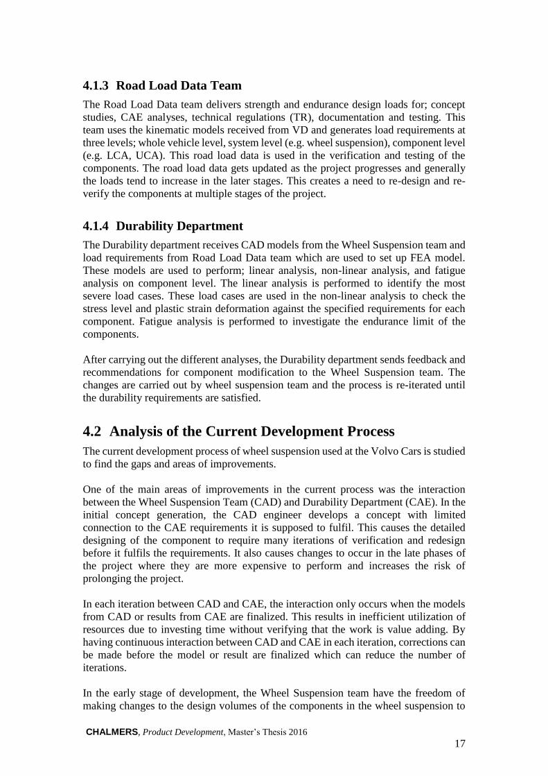
4.1.3 Road Load Data Team
The Road Load Data team delivers strength and endurance design loads for; concept
studies, CAE analyses, technical regulations (TR), documentation and testing. This
team uses the kinematic models received from VD and generates load requirements at
three levels; whole vehicle level, system level (e.g. wheel suspension), component level
(e.g. LCA, UCA). This road load data is used in the verification and testing of the
components. The road load data gets updated as the project progresses and generally
the loads tend to increase in the later stages. This creates a need to re-design and re-
verify the components at multiple stages of the project.
4.1.4 Durability Department
The Durability department receives CAD models from the Wheel Suspension team and
load requirements from Road Load Data team which are used to set up FEA model.
These models are used to perform; linear analysis, non-linear analysis, and fatigue
analysis on component level. The linear analysis is performed to identify the most
severe load cases. These load cases are used in the non-linear analysis to check the
stress level and plastic strain deformation against the specified requirements for each
component. Fatigue analysis is performed to investigate the endurance limit of the
components.
After carrying out the different analyses, the Durability department sends feedback and
recommendations for component modification to the Wheel Suspension team. The
changes are carried out by wheel suspension team and the process is re-iterated until
the durability requirements are satisfied.
4.2 Analysis of the Current Development Process
The current development process of wheel suspension used at the Volvo Cars is studied
to find the gaps and areas of improvements.
One of the main areas of improvements in the current process was the interaction
between the Wheel Suspension Team (CAD) and Durability Department (CAE). In the
initial concept generation, the CAD engineer develops a concept with limited
connection to the CAE requirements it is supposed to fulfil. This causes the detailed
designing of the component to require many iterations of verification and redesign
before it fulfils the requirements. It also causes changes to occur in the late phases of
the project where they are more expensive to perform and increases the risk of
prolonging the project.
In each iteration between CAD and CAE, the interaction only occurs when the models
from CAD or results from CAE are finalized. This results in inefficient utilization of
resources due to investing time without verifying that the work is value adding. By
having continuous interaction between CAD and CAE in each iteration, corrections can
be made before the model or result are finalized which can reduce the number of
iterations.
In the early stage of development, the Wheel Suspension team have the freedom of
making changes to the design volumes of the components in the wheel suspension to

18 CHALMERS, Product Development, Master’s Thesis 2016
improve the performance. But, at this stage, they do not have the knowledge on how to
change design volumes in order to improve it. This can be achieved through utilizing
the CAE knowledge to optimize the design volumes. However, when the components
are sent to be developed by a supplier, the design volume for that component has to be
locked which restrict the optimization of adjacent components. The design volume
optimization, therefore, has to be performed prior to sending it to a supplier.
Each department in the development process have a narrow view of the requirements
which each component has to fulfill. In the CAD department the requirements related
to packaging, kinematics, etc. are considered while in the CAE department the
considered requirements are related to stiffness, fatigue, etc. From a development point
of view each component has to fulfill all the requirements simultaneously and requires
collaboration and understanding of the overall requirements of each component which
is lacking in the current process. This reduces the department’s ability to provide
qualitative inputs to ease the work of other departments.
From conducting multiple interviews and discussions within same unit, it was identified
that the engineers had different understandings of the how the development is carried
out which indicates that the defined development process is not followed.

CHALMERS, Product Development, Master’s Thesis 2016 19
5 Proposed Development Process The proposed development process is developed by first investigating the current
process to find the requirements for the new process to fulfil. This chapter presents the
proposed development process of the wheel suspension together with the challenges
with replacing the current process.
5.1 Proposed Development Process
From the pilot study, it was identified that there was no common view of the overall
development cycle involving all the activities performed to develop a wheel suspension.
It was also identified that the concepts were developed with limited CAE knowledge
which caused it to be verified and updated in multiple iterations between CAD and CAE
before getting approved, see Figure 5.
Volvo Cars is a vehicle manufacturing company and when a similar scenario is
considered in a traffic situation, where all drivers follow different processes for driving
the vehicle, it is easy to imagine that this would end up in delays.
By developing a new process which structures the development of wheel suspension, it
is possible to reduce the lead time for the development work. A structured process is
also pre-requisite in developing cross-functionality between different departments.
Closer collaboration between CAD and CAE forms a basis for CAE driven
development. In the proposed process in this thesis, the CAE driven development is
done through implementing optimization in the early stages of the development.
Prior to the development of the new process, a list of requirements, shown below, which
the process needs to fulfil was generated through brainstorming and discussions with
experts.
The process should:
Be easy to adopt by the engineers.
Be realizable through the use of commercial software.
Be reproducible/adoptable for use to the varied set of components.
Fit in the existing process.
Include optimization into early stage of development.
Capture the required data and technical details.
Have defined deliverables.
Highlight key interactions between the involved units.
Be robust.

20 CHALMERS, Product Development, Master’s Thesis 2016
Figure 5 – Illustration of how the concepts are iterated between CAD and CAE
From the interviews with the CAD engineers, it was identified that the packaging
volume had become an increasing problem in recent projects due to increasing
complexity of the components in the wheel suspension. To solve this problem, the CAD
engineers needed a more efficient process to improve the design volumes of the
components in the wheel suspension. One way to obtain this, which is used in the
proposed process, is through creating a process where optimization is used for creating
the design volume of the component. Figure 6 shows the proposed process for the
development of components in the wheel suspension. The new proposed process for developing components of the wheel suspension is CAE
driven and involves a close collaboration between CAD and CAE. In the first step, the
CAD engineer creates design volumes for each component in the wheel suspension.
In the second step, optimization is used to balance the design volumes and a topology
optimization using simplified CAE requirements is performed inside each component.
The new optimized design volumes are used in kinematic simulations to verify the
clearance requirements and updated if this is not fulfilled.
When the clearance requirements are fulfilled, the design volumes are sent for detailed
optimization and concurrently the topology optimized models are used as an input for
developing early concepts for the components. The detailed optimization uses complete
CAE requirement to generate a detailed topology structure for each component. The
early concepts of the component are used for creating a first draft of the wheel
suspension which is checked against driving requirements.
Figure 6 - Illustrates the proposed development process of components in the wheel
suspension
CAD CAE
Detailed
Optimization
Model
Realization FEM
Verification
Early Concept
Creation
Design Volume
Optimization
and Validation
Design Volume
Creation
Initial Design
Volume Balanced
Design Volume
CHALMERS, Product Development, Master’s Thesis 2016 21
In the Model Realization step, the results from the detailed optimization will be used to
update the early concepts. The models are then realized using requirements from
manufacturing.
In the last step, the models are verified with FEM simulations and updates are iterated
with CAD engineers until the CAE requirements for each component are fulfilled.
5.2 Challenges for the New Development Process
This section focuses on analyzing the challenges which the new development process
will pose to be implemented at Volvo Cars. It also discusses the adaptability of the
process with the current situation at Volvo Cars and what changes needs to be done in
order to replace the current process with the proposed process.
Initial design volume creation for components using the kinematic simulation has been
carried out in earlier projects at Volvo Cars. The current way of performing this is time
consuming which causes it to be inefficient in a full scale project. However, projects
are currently carried out to make this process more automated which will decrease the
lead time for this activity.
Not all of the steps in the proposed development process have been carried out at Volvo
Cars and therefore, processes need to be created for these steps. One such process is the
optimization of design volumes which also needs to be verified before implementing it.
This process relies on the availability of function in the commercial software which is
currently limited in the field of design volume optimization.
In order to generate early concepts within the optimized design volumes, it is required
to perform a topology optimization. This topology optimization will be carried out in
the early stage of development which requires the simulation time to be low. In order
to achieve this, simplified CAE requirements has to be selected, which results in a good
representation of the detailed optimized results. This requires extensive testing to
identify these simplified CAE requirements.
The topology optimization on individual components are currently used in projects at
Volvo Cars. The process to carry out the detailed topology optimization is further
developed in ongoing projects. The major challenge is encountered in the realization
step from a topology optimized structure to manufacturable part. The development of
this has been initiated and will be further investigated in planned projects at Volvo Cars.
Volvo Cars have processes for virtual verification through FEA which is well-
established and can therefore be implemented into the proposed process. However, to
improve the overall process, an increased communication between CAD and CAE need
to be established.

22 CHALMERS, Product Development, Master’s Thesis 2016

CHALMERS, Product Development, Master’s Thesis 2016 23
6 Tests on Sample Components This chapter highlights the investigation carried out to solve the multi-component
design volume optimization through the use of the commercial software package
HyperWorks. The investigation is split into two sections one examining the method of
how to set up the model for a multi-component design volume optimization and the
other examines how to control the optimization process.
6.1 Simplified Model Setup
Design volume optimization of multiple components is a novel concept and methods to
achieve this through the use of commercial software is a developing field. To create a
method for Volvo cars to perform this, multiple approaches were generated through
brainstorming, practical use of the software and expert consultation from Altair
Engineering Inc. Two approaches were found to be potential candidates for solving the
design volume optimization problem.
In the first approach, see Figure 7, HyperMesh would be used to create and prepare the
FE models with boundary conditions, loadings, and material data. The models would
be morphed and dependencies would be created between the components using the
HyperMorph module in HyperMesh. The created models would be solved in OptiStruct
for shape and topology optimization and the results generated would then be post-
processed in HyperView, to interpret the optimized values for design volume
optimization.
In the second approach, see Figure 8, the creation and preparation of FE models in
HyperMesh would be similar to the first approach. Here, the shape optimization would
be controlled by HyperStudy and OptiStruct would be used to solve the topology
optimization. HyperView together with HyperStudy would be used to interpret and
generate the optimized values for design volume optimization.
Figure 7 - Illustrates the 1st approach to design volume optimization
HyperMesh
• FE Modeling
• Coupling Compoent using HyperMorph
OptiStruct
• Shape and Topology Optimization
HyperView
• Post Processing Results
• Interpreting optimized design volume results

24 CHALMERS, Product Development, Master’s Thesis 2016
Figure 8 - Illustrates the 2nd approach to design volume optimization
After evaluating the possibility of realizing the approaches it was found that the second
approach would require a longer investigation and implementation time since it
involves one more software compared to the first approach. It was also identified that
the first approach was more adaptable due to that it only uses one software for carrying
out the shape and topology optimization and it was therefore chosen for further
investigation.
In the early phases of verification and testing, models of the design volumes of the UCA
and LCA was obtained from the CAD department. However these models was
identified to have complex geometry in terms of small design features which would
introduce unnecessary difficulties in the pre-processing stage. It was therefore decided
to use simplified models in the early phases to reduce the time needed for pre-
processing and simulation time of each optimization run. The simplified models would
also make it easier to predict and understand the behavior of the models when different
settings were changed between the runs. They could also ease the decision on what
corrective actions to perform in order to obtain a satisfactory result. The simplified
models were also used to create a scenario representing the conflict between the UCA
and LCA in the S90/V90 configuration.
In the pre-processing the FE-models for the simplified UCA and LCA were created,
see Figure 9 and 10. The simplified models were split into design and non-design
volume. The design volume is the region where the topology is to be optimized. The
non-design space represents bushings and connection points etc. with predefined design
and therefore material is not allowed to be removed from these regions.
Figure 9 - Topology optimization settings of the simplified model of the LCA. The
picture shows how the model was split into design space and non-design space together
with the RBE:s, constraint, and force that were applied to the model.
HyperMesh
• FE Modeling
• Coupling Components using HyperMorph
HyperStudy
• Controlisg FE model's shape design variables
OptiStruct
• Topology Optimization
HperView
HyperStudy
• Post Processing Results
• Generating optimized design volume from HyperStudy
Design volume RBE:s
Constraint
Force
Non-design volume

CHALMERS, Product Development, Master’s Thesis 2016 25
Figure 10 - Topology optimization settings of the simplified model of the UCA. The
pictures shows how the models was split into design space and non-design space
together with the RBE:s, constraint, and force that were applied to the model.
The UCA and LCA used in the S90/V90 configuration are made of casted aluminum
and this is also the material used in the FE-models. The mesh type used on the
simplified models was tetrahedral mesh of size 5mm. This corresponds to the mesh-
guidelines, used to set up the models of the UCA and LCA, for linear static testing at
Volvo Cars. In the models RBE:s (rigid body elements) are used to represent the
attachment points of the components. For the simplified models, two clusters of RBE:s
were created from the nodes on the interior surface of the holes to a node created at the
center of each hole. At these center nodes the boundary conditions, forces, and
optimization constraints are applied.
In the early phases of verification, the durability department performs static linear-
simulations where the components are tested against predefined stiffness requirement
specific for each component. For the optimized model to fulfill the predefined stiffness
requirements, a unit force and a displacement constraint was applied see Table 1. The
displacement constraint for the optimizations was set in the node where the force is
applied in the direction of the force. The trend in the automotive industry towards
developing lighter vehicles is the reason for choosing minimize mass as the objective
function in the optimization.
Constraint
RBE:s
Design volume
Force
Non-design volume

26 CHALMERS, Product Development, Master’s Thesis 2016
Table 1 – Shows the boundary and loading conditions of the simplified UCA and
LCA.
Model Constraint Force Displacement
Constraint
Objective
Function
Simplified
UCA Fully fixed 1kN 0.3 mm
Minimize
mass
Simplified
LCA Fully fixed 1kN 0.1 mm
Minimize
mass
To identify potential improvements in the design volume of the component, the result
from topology optimization was studied to locate the high density regions. These
regions indicate that a higher fraction of load is transferred through these elements
compared to other regions in the structure. The loads in these elements can be lowered
through expanding the design volume at these regions. By decreasing the loads, a lighter
topology structure can be obtained.
From the result of the topology optimization it was evident from the high density
regions that weight savings could be obtained from expanding the simplified UCA’s
top and bottom surface, see Figure 11. But the top surface of the UCA is limited by a
body beam and since this thesis is limited to the components within the wheel
suspension, focus is put on the high density region in the bottom surface of the model.
The high density region in the bottom surface is where the design volume will be
increased in the simultaneous shape and topology optimization. In the simplified LCA
the high density region was identified at the top and bottom surface, see Figure 12. The
bottom surface of the LCA is restricted by the ground clearance which is why the top
surface was used in the simultaneous shape and topology optimization.
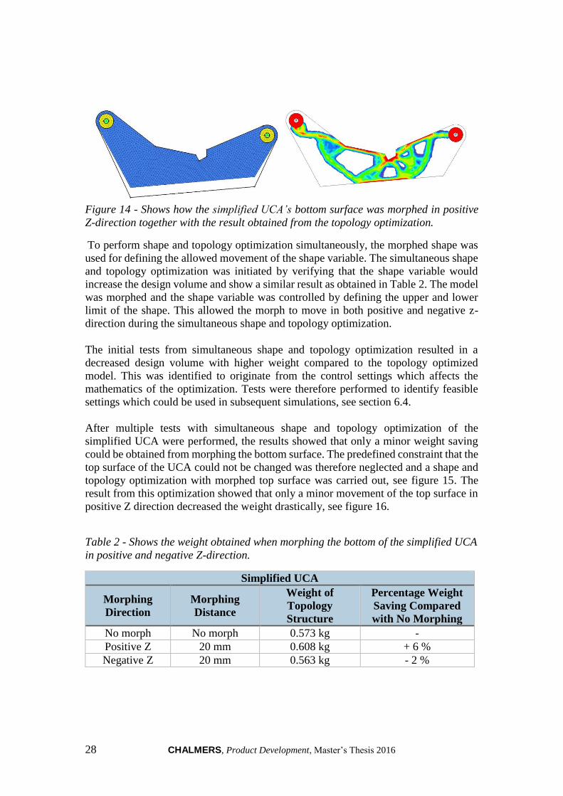
Figure 11 - Topology optimization result of the simplified UCA

CHALMERS, Product Development, Master’s Thesis 2016 27
Figure 12 - Topology optimization result of the simplified LCA
6.2 Shape and Topology Optimization
The next step in the testing was to morph the models in the regions and directions where
the models showed potential for weight savings. To enable morphing a morphing
domain had to be chosen. The morphing domain contains the elements that will share
the impact of the shape change. For the simplified models the design volume, see Figure
9 and 10, was chosen as morphing domain. The top surface of the simplified UCA and
the bottom surface of the simplified LCA was chosen as morphing surfaces.
Next the simplified UCA’s bottom surface was morphed in both positive and negative
Z direction in two separate models, see Figure 13 and 14, to verify that the model with
increased design volume would result in a lighter result after optimization. The result
from the topology optimization is shown in Table 2, which illustrates that increasing
the design volume in the high density element region reduced the weight.
Figure 13 - Shows how the simplified UCA’s bottom surface was morphed in negative
Z-direction together with the result obtained from the topology optimization.
28 CHALMERS, Product Development, Master’s Thesis 2016
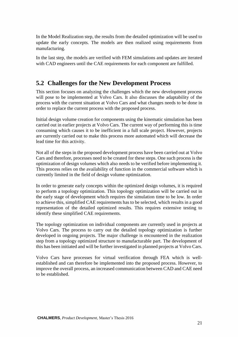
Figure 14 - Shows how the simplified UCA’s bottom surface was morphed in positive
Z-direction together with the result obtained from the topology optimization.
To perform shape and topology optimization simultaneously, the morphed shape was
used for defining the allowed movement of the shape variable. The simultaneous shape
and topology optimization was initiated by verifying that the shape variable would
increase the design volume and show a similar result as obtained in Table 2. The model
was morphed and the shape variable was controlled by defining the upper and lower
limit of the shape. This allowed the morph to move in both positive and negative z-
direction during the simultaneous shape and topology optimization.
The initial tests from simultaneous shape and topology optimization resulted in a
decreased design volume with higher weight compared to the topology optimized
model. This was identified to originate from the control settings which affects the
mathematics of the optimization. Tests were therefore performed to identify feasible
settings which could be used in subsequent simulations, see section 6.4.
After multiple tests with simultaneous shape and topology optimization of the
simplified UCA were performed, the results showed that only a minor weight saving
could be obtained from morphing the bottom surface. The predefined constraint that the
top surface of the UCA could not be changed was therefore neglected and a shape and
topology optimization with morphed top surface was carried out, see figure 15. The
result from this optimization showed that only a minor movement of the top surface in
positive Z direction decreased the weight drastically, see figure 16.
Table 2 - Shows the weight obtained when morphing the bottom of the simplified UCA
in positive and negative Z-direction.
Simplified UCA
Morphing
Direction
Morphing
Distance
Weight of
Topology
Structure
Percentage Weight
Saving Compared
with No Morphing
No morph No morph 0.573 kg -
Positive Z 20 mm 0.608 kg + 6 %
Negative Z 20 mm 0.563 kg - 2 %

CHALMERS, Product Development, Master’s Thesis 2016 29
Figure 15 - Shows how the simplified UCA's top surface was morphed in positive Z-
direction together with the result obtained from the topology optimization
Figure 16 - Graphical representation of the weight saved from bottom and top surface
morphing
A similar investigation was carried out to gain knowledge about the behavior of shape
and topology optimization of the simplified LCA which was used together with the
simplified UCA in the simplified combined model.
6.3 Combined Model Optimization
Once the result for the individual models were obtained and the weight saving potential
were identified, the next step was to couple the two models into one combined model.
The two simplified models were imported into a single model. A coupling was made to
maintain the minimal distance between the two models. To obtain the coupling, a
dependency between the morphed surfaces was created. Using this dependency, a shape
was created such that, when the shape of one model was changed, the other model’s
shape changed accordingly.
0%
5%
10%
15%
20%
25%
30%
5 10 15 20 30
Wei
gh
t S
av
ing
Morphing Distance (mm)
Weight Saving Potential Comparision of Morphing
the Simplfied UCA's Top and Bottom Surface
Bottom surface Top Surface

30 CHALMERS, Product Development, Master’s Thesis 2016
As shown in Figure 17, the top surface of the simplified LCA were coupled with the
bottom surface of the simplified UCA. Figure 18 shows the shape change for the
coupled model in positive and negative z-direction which was used for creating the
shape variable in the optimization. The boundary conditions, loading conditions and
constraints were kept from the individual models. Design variable for topology was
created by selecting the design volume property of both the individual models. The
objective for the simplified combined model was to minimize the total mass of the two
models.
Figure 17 – Illustration of the coupled surfaces in the simplified combined model,
used in the shape and topology optimization
Figure 18 - Illustrates how the simplified combined model was morphed in positive
and negative Z-direction
Coupled surfaces

CHALMERS, Product Development, Master’s Thesis 2016 31
The results from the shape and topology optimization of the simplified combined model
showed that the optimal shape was obtained when the design volume of the simplified
LCA increased and the simplified LCA’s design volume decreased, see Figure 19. The
identified reason for the simplified LCA to increase its design volume is that this was
more beneficial in terms of weight saving compared to increasing the design volume of
the simplified UCA.
Figure 19 – Result obtained from the shape and topology optimization of the simplified
combined model.
Table 3 - Shows the weight obtained when performing topology optimization topology
optimization compared to performing combined shape and topology optimization of the
simplified UCA and LCA.
Model Optimization Type
Weight of
Topology
Structure
Total Weight
Simplified UCA Topology 0.577 kg 1.083 kg
Simplified LCA Topology 0.506 kg
Simplified
Combined Model Shape and Topology 1.073 kg 1.073 kg

32 CHALMERS, Product Development, Master’s Thesis 2016
6.4 Control Setting Test for Shape and Topology
Optimization
Optimization control settings allows the user to set the value for different control
parameters which will override the default setting for that parameter in the optimization.
By doing so, the user is allowed to customize the optimization for a specific purpose.
In this thesis, it was of interest to find the effects of different parameters on the output
of the simultaneous shape and topology optimization. The method used for testing the
control setting was OFAT (One factor at a time), where one parameter was changed at
a time and the result which it produced was observed. The section below presents the
different control settings which were tested.
6.4.1 DESMAX
DESMAX in HyperMesh is used to control the maximum allowed iterations the solver
can run before the optimization is terminated. If the user is only interested in a coarse
topology of the component, DESMAX can be set low to keep the simulation time low.
The default value of DESMAX is 30, which caused the solver to terminate the
simultaneous shape and topology optimization before the solution had converged.
Because of the non-converged result, the optimized models resulted in a decreased
design volume with an increased weight compared to the result from only topology
optimization. Therefore, this control parameter was further investigated with a higher
value to see if the result would be different if it was allowed to converge.
By setting the DESMAX to a higher value, the result converged in the simultaneous
shape and topology optimization of the simplified models. The converged result had
both an increased design volume and decreased weight compared to the result from
only topology optimization. This control parameter was therefore continuously changed
throughout the testing to ensure that the optimization reached convergence.
6.4.2 OBJTOL
The control parameter OBJTOL is the relative convergence criterion of the objective
function which describes how similar two successive iterations of the optimization
should be for the solver to treat the optimization as converged. If the value of this
parameter is lowered, the convergence criterion becomes tighter which drives the solver
to find a result closer to the optimal design. Lowering the value of this parameter,
increases the number of iterations needed for the optimization to converge which
prolongs the simulation time.
During the post-processing of the tests on the simplified models, it was identified that
the design volume still increased during the last iterations of the optimization. The
OBJTOL parameter was set to a lower value than the default to investigate if the design
volumes would continue to expand and generate a lighter result. The result showed that;
the design volume increased, the weight was reduced and the design volume change
became asymptotic with respect to the iterations.

CHALMERS, Product Development, Master’s Thesis 2016 33
6.4.3 MINDENS
The control parameter MINDENS controls the minimum element density that is
allowed for any element in the optimization. This parameter was investigated to see if
the design volume would increase, if a lower value was set compared to the default
value. It was also of interest to identify how much weight the minimum density
elements added to the optimized result. The result from this investigation showed that
when a lower value of the parameter was used, the design volume converged at a larger
increase in design volume. The weight of the component was also lowered considerably
and therefore this parameter was kept lower than the default value in the subsequent
simulations.
6.4.4 MATINIT
The post-processing of the test on the simplified components showed that the design
volume decreased during the initial iterations, then increased in later iterations, and
finally converged at an increased design volume compared to the starting point of the
optimization. The reason for this behavior was identified to be the high initial density
which fulfilled the stiffness constraints and since the objective was to decrease mass,
the most efficient way was through decreasing the design volume. Therefore, the
parameter MATINIT which defines the initial element densities was investigated to see
if this behavior could be avoided.
The value for MATINIT was lowered and the result showed that the design volume
grew continuously during the initial iterations. When the value of MATINIT was
decreased, the stiffness constraints were no longer fulfilled and therefore the design
volume was instead increased in the initial iterations. From these results, it was decided
to have a low value of MATINIT throughout the tests.
6.4.5 Algorithm
There are three algorithms available in HyperMesh to solve an optimization problem;
sequential quadratic programming (SQP), the method of feasible directions (MFD), and
DUAL. SQP is a gradient-based iterative optimization method which is generally used
for nonlinear problems. MFD is based on the principle to iteratively move from one
feasible design to an improved feasible design where the objective function is reduced
as long as the constraints at the new design point is not violated. The DUAL algorithm
is based on separable convex approximation and it is used for problems involving
multiple design variables.
In the testing of the simplified UCA, different algorithms were applied and the result
obtained from each different algorithm did not vary significantly. It was, therefore,
decided to keep the algorithm settings to MFD, which is the default, for subsequent
testing.
6.4.6 DISCRETE
In general, the result from a topology optimization contains large volumes of
intermediate densities. From such results, it can be difficult to distinguish which regions
of the topology should contain material and what regions should be treated as holes.
Therefore, penalty techniques need to be introduced to force the final design to be

34 CHALMERS, Product Development, Master’s Thesis 2016
represented by densities closer to 0 or 1 for each element. The penalization technique
used in OptiStruct is the "power law representation of elasticity properties," which can
be expressed as follows:
Ḵ(𝜌) = 𝜌𝑃𝐾
Where, Ḵ and K represent the penalized and the real stiffness matrix of an element,
respectively, ρ is the density and P is the penalization factor.
The discreteness parameter influences the size of the penalization and by increasing its
value the number of elements that remain between 0 and 1 can be reduced.
The result from the optimization tests of the sample models showed that many of the
elements had intermediate densities between 0 and 1. This was identified to introduce
difficulties in the design realization of the optimized part. The discrete parameter was
investigated to identify if a more prominent design could be obtained from increasing
the penalty factor. The result from this investigation showed that the simultaneous
shape and topology optimization with an increased penalty converged at a smaller
design volume compared to keeping it at its default value. This also increased the
weight of the optimized component and the default value was therefore used in
subsequent simulations.
6.4.7 Member Size Control
The member size control settings provide the functionality to prevent the generation of
small or large beams in the topology optimized structure. In HyperMesh, the MINDIM
parameter is used to control the smallest allowed beam size and MAXDIM is used to
control the largest allowed beam size. Through controlling the beam size, these
parameters can be used to generate an optimized topology for a specific manufacturing
process.
For the simplified UCA, different values for MINDIM were tested in order to determine
the impact it would have on the shape and topology optimization. Figure 20 shows the
topology obtained for the simplified UCA when a MINDIM of 30 was used and Figure
21 the topology when a value of 5 was used.
When MINDIM was used in the optimization, a more prominent topology was
obtained. As the value of MINDIM was increased, the design volume of the model
decreased which caused the weight of the structure to increase (See picture). To find
the optimal value of MINDIM for the specific manufacturing process required a
thorough investigation, and was therefore not included in the subsequent testing.
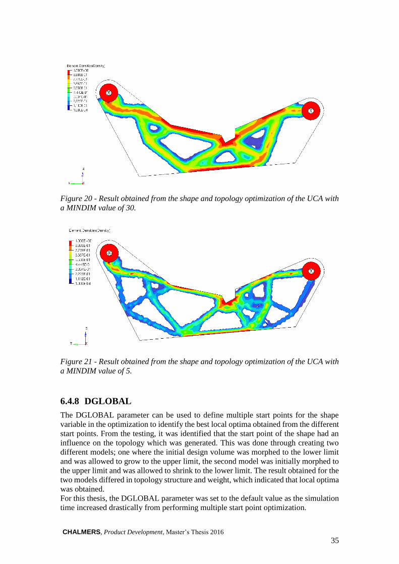
CHALMERS, Product Development, Master’s Thesis 2016 35
Figure 20 - Result obtained from the shape and topology optimization of the UCA with
a MINDIM value of 30.
Figure 21 - Result obtained from the shape and topology optimization of the UCA with
a MINDIM value of 5.
6.4.8 DGLOBAL
The DGLOBAL parameter can be used to define multiple start points for the shape
variable in the optimization to identify the best local optima obtained from the different
start points. From the testing, it was identified that the start point of the shape had an
influence on the topology which was generated. This was done through creating two
different models; one where the initial design volume was morphed to the lower limit
and was allowed to grow to the upper limit, the second model was initially morphed to
the upper limit and was allowed to shrink to the lower limit. The result obtained for the
two models differed in topology structure and weight, which indicated that local optima
was obtained.
For this thesis, the DGLOBAL parameter was set to the default value as the simulation
time increased drastically from performing multiple start point optimization.

36 CHALMERS, Product Development, Master’s Thesis 2016

CHALMERS, Product Development, Master’s Thesis 2016 37
7 Design Volume Optimization Process This chapter contains a detailed process developed for simultaneous optimization of
multiple components. This process was developed based on the knowledge gained from
the simple component testing and contains stepwise process to carry out the
optimization. The process was tested and further developed during the verification
stage, where it was used to optimize the design volumes of the UCA and LCA in the
S90/V90 configuration.
An IDEF0 diagram is used to represent the new process at different abstraction levels.
In the top level, the main function of the process is represented which is split into four
sub-functions representing the main tasks to be carried out in the process. The sub-
functions are further divided into activities to be performed to achieve each main task.
This process is developed through using the features available in HyperWorks, but it
can be adopted to other software.
7.1 Design Volume Optimization
The main function of the process, design volume optimization, is represented by Node
A0 in the IDEF0 diagram, shown in Figure 22. The main inputs to this function are
initial design volume, and CAD and CAE data. The CAD and CAE data includes,
guidelines, boundary & loading conditions, material properties, and manufacturing
constraints etc. The process is controlled by the optimization guidelines produced
during this thesis. The mechanisms needed to carry out this process are man-hours from
CAD & CAE engineers and the software package HyperWorks. This process generates
two outputs; an optimized design volume for each component, and concept geometries
which includes a topology optimized part geometry in the optimized design volume.
These outputs will be sent to the CAD department where the new concept geometry
will be verified against the requirements of the part. If the concept geometry passes the
verification stage it will serve as a basis for developing a concept geometry to be used
in the early stages of development and the design volume will be sent to the CAE
department for detailed optimization.

38 CHALMERS, Product Development, Master’s Thesis 2016
Figure 22 - Shows the IDEF0 diagram at node A0 illustrating is the main function of
the process.
7.2 Sub-functions for Deign Volume Optimization
Figure 23 shows second level of the IDEF0 diagram where the main function at node
A0 was divided into four sub-functions, FE Modeling, Topology Optimization, Shape
and Topology Optimization, and Combined Optimization, which are described in the
sections below. If the execution of any of the sub-functions are unsatisfactory due to
mesh failure, geometry irregularity or morphing errors etc., a design change feedback
is sent to CAD engineer. The CAD engineer will update the CAD model based on the
dialogue and the steps prior to the sub-function where the error occurred will be re-
performed.

CHALMERS, Product Development, Master’s Thesis 2016 39
Figure 23 - Shows the second level of the node A0 in theIDEF0 diagram, illustrating
the four sub-functions of the process; FE Modeling, Topology Optimization, Shape and
Topology Optimization, and Combined optimization.
7.2.1 FE Modeling
The inputs to this sub-function are the initial design volume of the component, and
CAD and CAE data. At this step a FE model for each component will be generated,
which consist of; mesh, boundary conditions, loading conditions, material properties,
and design and non-design volume.
7.2.2 Topology Optimization
The FE model generated at the previous step is used along with optimization data (e.g.,
Stiffness constraint, objective function), to set up a topology optimization for each
component. The topology optimization is executed and the results are post-processed
to identify the regions to be morphed in the shape & topology optimization. The output
from this step also consist of a FE model with topology optimization settings for each
component.
7.2.3 Shape and Topology Optimization
The input to this sub-function are; FE model with topology optimization setup and
knowledge about regions to be morphed for creating shapes. Each individual
component will be morphed depending on the results from the previous step and shape
variables will be created. Simultaneous shape and topology optimization will be
executed for each component and the results from this process will give the knowledge
about the behavior of the components. Another output will be a FE model with shape
and topology optimization setup.

40 CHALMERS, Product Development, Master’s Thesis 2016
7.2.4 Combined Optimization
In this sub-function each FE model with optimization setting will be merged together
into one combined model. The combined model will be morphed with couplings
between the components and from this new shape variables will be created. This
process generates two outputs; an optimized design volume for each component, and
concept geometries which includes a topology optimized part geometry in the
optimized design volume.
The sublevel present in the above process can be further split into further detailed
sublevels to define specific tasks. The next section will discuss the guidelines and
process for each sublevel node.
7.3 FE Modeling
Figure 24 represents the activities performed in the sub-function FE Modeling in the
third level of IDEF0 diagram. The process is divided into four activities; Data
collection, Geometry handling, Mesh creation, and Boundary conditions and load setup
which will be discussed into the following sections.
Figure 24 - Shows the third level of the IDEF0 diagram at node A1, illustrating the
activities performed in the sub-function FE Modeling.

CHALMERS, Product Development, Master’s Thesis 2016 41
7.3.1 Data Collection
Data collection deals with collecting data required for FE modeling and optimization
setup. The data consists of;
initial design volume of each component,
defined design and non-design volumes,
hard points,
material properties,
CAE requirements specific for each component,
manufacturing requirements,
optimization and mesh guidelines.
The guideline for obtaining this data is shown in Appendix 1.
7.3.2 Geometry Handling
This activity deals with cleaning up the geometry model and making it suitable for
generating a mesh. Cleaning up of the geometry involves removing unnecessary edges,
lines, etc. from the geometry model which will increase the quality of the mesh in the
next step. Geometry handling also include dividing the geometry into design and non-
design volume and adding a material property to the respective entity. Refer Appendix
2 shows in detail how the geometry handling is carried out in HyperMesh.
7.3.3 Mesh Creation
In Mesh Creation, the geometry obtained from previous step is used to generate the
mesh as defined in the guideline, see Appendix 3. There are multiple ways to create
mesh for a solid component and depending on the complexity of geometry, different
methods from the guideline can be adopted. In this activity, the mesh should also be
tested by running the “check” simulation. The “check” simulation is used to verify the
inputs of the FE model.
7.3.4 Boundary Condition and Load Setup
This activity involves setting up boundary and loading conditions for each component
in the FE model together with connections at different loading point, see Appendix 4.
These connections are created to closer represent the conditions in the physical
component. The last step in this activity is to verify the inputs of FE model by running
the “check” simulation.
7.4 Topology Optimization
The sub-function Topology Optimization is split into Topology Optimization Setup &
Execution and Topology Optimization Post Processing, see Figure 25. The section
below describes the activities carried out for performing topology optimization of each
component.

42 CHALMERS, Product Development, Master’s Thesis 2016
Figure 25 - Shows the third level of the IDEF0 diagram at node A2, illustrating the
activities performed in the sub-function Topology Optimization.
7.4.1 Topology Optimization Setup & Execution
In this activity, the optimization data obtained from the previous step is used to set up
the responses, objective function, and constraint for the topology optimization. The
design variable for the topology is defined in the model and control settings are applied
according to the guideline in Appendix 5. Each model are sent to the solver for topology
optimization and the results are sent for post processing.
7.4.2 Topology Optimization Post Processing
The post processing is used to interpret the results from the topology optimization of
each individual component and performed using post processing guidelines, see
Appendix 7. The result obtained is checked for convergence to verify that the result has
fulfilled all the constraint. The performance of the topology optimized structure
obtained is noted down for each component to be used for comparison in later activities.
The potential morphing regions are identified by locating the high density regions in
the topology structure which indicates potential increase in performance. These
potential morphing regions are checked against the geometrical constraints for each
component to find where the optimization of design volume should be performed. The
identified morphing regions together with the FE model with topology optimization
settings will be used in the next step for performing shape and topology optimization.

CHALMERS, Product Development, Master’s Thesis 2016 43
7.5 Shape and Topology Optimization
In this section, the three activities; Morph Setup, Shape and Topology Optimization
Setup & Execution, and Shape and Topology Post Processing which are part of sub-
function Shape and Topology Optimization are described, see Figure 26.
Figure 26 - Shows the third level of the IDEF0 diagram at node A3, illustrating the
activities performed in the sub-function Shape and Topology Optimization.
7.5.1 Morph Setup
This activity is performed to create a morphing domain and shape for each model from
the morphing regions identified in the previous step, see Appendix 6. The morphing
domain defines the elements which will share the impact of the morphing. The
morphing is controlled by handles which are automatically created at the edges of the
geometry. By moving the handle in the identified morphing regions, shapes are created.
The valid range for positive and negative morphing distance should be defined for each
shape of each component. The created shapes together with valid range for morphing
distance is used in the next activity to set up the simultaneous shape and topology
optimization.
7.5.2 Shape and Topology Optimization Setup & Execution
In the simultaneous shape and topology optimization, the settings for the topology
optimization are kept from the previous model. The shape variable for this optimization
is created from the shapes obtained from the previous activity, see Appendix 5. The
limits of the shape variable are defined using the values of the valid range of morphing
distance for each shape. The shape variable allows the design volume of the model to
changes within the defined limits.

44 CHALMERS, Product Development, Master’s Thesis 2016
From the simultaneous shape and topology optimization, the optimal shapes are found
through optimizing the topology which identifies if the design volume should grow or
shrink at each iteration until the optimization is terminated. These results are sent for
post processing.
7.5.3 Shape and Topology Optimization Post-processing
The post processing is used to interpret the results from the shape and topology
optimization of each individual component and performed using post processing
guidelines, see Appendix 7. The result obtained is checked for convergence to verify
that the result has fulfilled all the constraint.
In order to identify the increase in performance, the performance of the shape and
topology optimized structure of each component is compared with the performance of
the topology optimization structure obtained at Node A22. If multiple shapes are used
in the optimization for a component, the shape with most performance improvement
potential should be noted together with the direction of shape change to be used when
setting up and verifying the combined model.
7.6 Combined Optimization
This sub-function cover the setup of the combined model where multiple models will
be imported into one single model and linked together using dependencies. The sub-
function is divided into three activities; Combined Model Morph Setup, Combined
Model Shape and Topology Optimization Setup & Execution, and Combined Model
Post Processing, see Figure 27.
Figure 27 - Shows the third level of the IDEF0 diagram at node A4, illustrating the
activities performed in the sub-function Combined Optimization.

CHALMERS, Product Development, Master’s Thesis 2016 45
7.6.1 Combined Model Morph Setup
The FE models of multiple components are imported into one single model where the
distance between the models represents the minimum allowed clearance between the
components. The shapes of the individual model are replaced with combined shapes. In
order to create combined shapes, the morphing domain of the individual models are
linked through creating dependencies between the handles, see Appendix 6. The
dependencies between the handles are created according to the conflicting regions
between the design volumes of two components. The conflicting region are in turn
determined by comparing the shape behavior of the individual result obtained at Node
33 to identify where the two components are limiting each other’s design spaces. The
combined model can consist of conflicting and non-conflicting shapes which can be
optimized simultaneously.
The valid range for positive and negative morphing distance should be defined for each
shape of the combined model. The created shapes together with valid range for
morphing distance is used in the next activity to define the shape variables for the
combine optimization.
7.6.2 Combined Model Shape and Topology Optimization Setup &
Execution
In the combined shape and topology optimization, the design variable for topology from
each individual component is replaced with a combined variable which contains the
design volume of all components in the model. The shape variable for each individual
component is replaced by shape variables created using the combined shapes obtained
from the previous activity, see Appendix 5. The limits of the shape variables are defined
by using the values of the valid range of morphing distance for each combined shape.
The objective function for each component in the combined model is replaced with an
objective which includes all the components.
From the combined shape and topology optimization, the optimal shape is found
through balancing the design volumes of the components in the combined model. The
balancing of the design volumes is determined by the shape and topology changes
which improve the objective function defined for the combined model. These results
are sent for post processing.
7.6.3 Combined Model Post Processing
This combined model post processing activity is used to first interpret and verify the
outputs from the combined optimization and then to deliver an optimized design
volume for each component, and concept geometries which includes a topology
optimized part geometry in the optimized design volume see Appendix 7.
In the verification step, the obtained result is checked for convergence to verify that the
result has fulfilled all the constraints. In order to identify the increase of performance
this process achieved, the combined performances of the optimized components in the
combined model are compared with the sum of the individual performance obtained
from the topology optimized structures obtained at Node A22.

46 CHALMERS, Product Development, Master’s Thesis 2016
The optimized design volume for each component can be delivered in multiple ways,
for example through exporting morphed geometries from HyperMesh, or a description
on how to update the CAD geometry with input from the morphed region and the result
of the end distance of the morph.
The topology optimized structure to be used for generating an early concept geometry
is exported by creating an STL file for a particular ISO value.

CHALMERS, Product Development, Master’s Thesis 2016 47
8 Verification of the Design Volume
Optimization Process This chapter covers the verification of the developed design volume optimization
process and discusses the findings from the implementation of the process in a real case
scenario. This chapter is divided into two sections, the first section consists of the
execution of the developed process for design volume optimization of the LCA and
UCA in the S90/V90 configuration. In the second section the design volume
optimization process is evaluated when performed to optimize the models in the real
case scenario.
8.1 Execution of the Design Volume Optimization
This section describes the execution of the Design Volume Optimization process when
applied to optimize the design volumes of the UCA and LCA in the S90/V90
configuration. The process consists of four sub-functions; FE Modeling, Topology
Optimization, Shape and Topology Optimization, and Combined optimization.
8.1.1 FE Modeling
The CAD models for the initial design volumes of the UCA and LCA together with
other necessary data was gathered to set up the models. The models were divided into
design and non-design volumes followed by geometry cleaning, meshing and
application of loading and boundary conditions.
Figure 28 shows the model setup of the UCA, the load and constraints for the model
are presented in Table 4. The loading in the model is applied in the local z-direction
which is where the stiffness requirement was calculated. Figure 29 shows the model
setup of the LCA, in this model, three different load steps are used to enable the
calculation of three different stiffness requirements, see Table 4.
Figure 28 - Shows the model setup to the UCA.
Design volume
Non-design volume
RBE:s Pt7
Pt1

48 CHALMERS, Product Development, Master’s Thesis 2016
Figure 29 – Shows the model setup of the LCA.
Table 4 - Shows the constrained Degrees Of Freedom (DOFs, loads, and
requirements for the hard points in the LCA and UCA.
Model
Hard
Point
Constrained
DOFs Load
Stiffness
Requirement
UCA
Pt 1 Local 1,2,3,6 -
Pt 7 Local 1,2 1 kN (Local z-
direction) 20 kN/mm
LCA
Pt 3 2,3 - -
Pt 4 1,2,3 - -
Pt 6 3 - -
Pt 18 - 1 kN (Z-direction) 3 kN/mm
Pt 56 - 1 kN (Z-direction) 25 kN/mm
Pt 68 - 1 kN (Z-direction) 10 kN/mm
The “check” simulation was used to verify the FE models and the models were sent for
topology optimization setup in the next sub-function.
8.1.2 Topology Optimization
In this sub-function, the topology optimization was set up for each model with data
collected in the previous sub-function. Responses, constraints and objective function
was defined for each model, see Table 5. The displacement constraint together with the
unit load represents the stiffness requirements for each model. Minimize mass was
chosen as the objective function for the models as the targeted weight for wheel
Pt3
Pt68
Pt6
Pt56
Pt18
Pt4
Design Volume
Non-design Volume

CHALMERS, Product Development, Master’s Thesis 2016 49
suspension components are continuously lowered and the potential weight reduction
was therefore of interest.
Table 5 - Shows the responses, constraints, and objective function used in the
optimization of the LCA and UCA.
Model Response
Type Response Location
Constraint Value
Objective Function
UCA Mass Design Volume - Minimize mass
Displacement Pt 7, Local DOF 3 0.05 mm -
LCA
Mass Design Volume - Minimize mass Displacement Pt 18, DOF 3 0.33 mm - Displacement Pt 56, DOF 3 0.04 mm - Displacement Pt 68, DOF 3 0.10 mm -
Figures 30 and 31 shows the results for the topology optimization of UCA and LCA
respectively. The optimized weights of the topology structure for each model is noted
down to be used as a datum for comparison in later stages, see Table 6.
In the topology structure of the models, the UCA’s bottom and top surfaces as well as
the LCA’s top surface were identified as potential morphing regions, as these contained
high density elements. These identified regions will be used to define the shapes in the
simultaneous shape and topology optimization for each model.
Figure 30 - Shows the topology optimization results of the UCA, used to identify high
density regions.

50 CHALMERS, Product Development, Master’s Thesis 2016
Figure 31 – Shows the topology optimization results of the LCA, used to identify high
density regions.
8.1.3 Shape and Topology Optimization
The design volumes of the UCA and LCA were chosen as morphing domains which
were used to create the shapes in the model.
In the UCA, two shapes were created from the previously identified morphing regions,
one on the top surface and another on the bottom surface of the model. The top surface
was constrained by a body beam which is not a part of the wheel suspension and could
therefore not be changed within the scope of this thesis. But, the topology structure
showed a weight saving potential in the top surface region, it was therefore chosen to
investigate this.
Figure 32 shows the limits of the shape variable defined for the bottom surface of the
UCA which was used in the simultaneous shape and topology optimization. The result
from the simultaneous shape and topology optimization is presented in Figure 33 which
indicates the design volume of the model was increased to save weight. From the post
processing, it was identified that the design volume increased to the maximum allowed
morphing distance which indicated that a lighter result could be obtained by increasing
the allowed morphing distance.
Figure 32 - Illustrates the shape limits of the bottom surface of the UCA in the shape
and topology optimization.

CHALMERS, Product Development, Master’s Thesis 2016 51
Figure 33 - Illustrates the obtained shape and topology optimization result when
allowing shape change in the bottom surface of the UCA.
The limit of the shape variable for the top surface morph of the UCA is shown in Figure
34. The result from the simultaneous shape and topology optimization for the top
surface showed a greater weight savings compared to the morphing the bottom surface,
see Figure 35. This was therefore further investigated by performing multiple
optimizations at different allowed morphing distances for each shape and the
comparison is shown in Figure 36.
Figure 34 - Illustrates the shape limits of the top surface of the UCA in the shape and
topology optimization.

52 CHALMERS, Product Development, Master’s Thesis 2016
Figure 35 - Illustrates the obtained shape and topology optimization result when
allowing shape change in the top surface of the UCA.
Figure 36 - Graphically illustrates the weight saving potential when morphing the top
compared to the bottom surface of the UCA.
The morphing limits of the shape variable for the top surface of the LCA is shown in
Figure 37 and 38. From the figure it can be seen that only a small morphing distance
was allowed in negative Z-direction which was due to limitations caused by the non-
design volume. In the post processing of the result from the simultaneous shape and
topology optimization, it was identified that the optimal result within the allowed
morphing range was obtained by increasing the design volume to the maximum limit,
see Figure 39.
0%
10%
20%
30%
40%
50%
60%
70%
5 10 15 20 30
Per
cen
tag
e W
eig
ht
Sa
vin
gs
Morphing Distance (mm)
Weight Saving Potential Comparision of Morphing
the UCA's Top and Bottom Surface
Bottom surface Top Surface

CHALMERS, Product Development, Master’s Thesis 2016 53
Figure 37 - Illustrates the shape limit in negative Z-direction of the top surface of the
LCA in the shape and topology optimization.
Figure 38 - Illustrates the shape limit in positive Z-direction of the top surface of the
LCA in the shape and topology optimization.
Figure 39 - Illustrates the obtained shape and topology optimization result when
allowing shape change in the top surface of the LCA.

54 CHALMERS, Product Development, Master’s Thesis 2016
The optimal morphing direction for each shape was noted down and used in the
verification of the combined shape and topology optimization.
8.1.4 Combined Optimization
The models of the LCA and UCA were imported into a single model to perform the
balancing of the components design volumes. For the combined optimization, the
objective function was defined to minimize the total mass of the two models. The next
step was to identify the conflicts between the models which was performed through
finding the morphed regions which were constrained by the other model. A conflict
region was identified between the top surface of the LCA and the bottom surface of the
UCA. These conflicting regions were coupled by creating dependencies between the
handles controlling the two surfaces in order to create a shape variable. Figures 40 and
41 shows the limits of the shape variable in negative and positive Z-direction
respectively, which the design volumes were allowed to change during the combined
shape and topology optimization.
The optimized topology structure of the combined model showed that the design
volume of the LCA had increased which forced the design volume of the UCA to
decrease, see Figure 42. The reason for this was identified to be that the LCA saved
more weight compared to the UCA by increasing its design volume. This conclusion
was drawn from comparing the weights of the individual models after topology
optimization with the results from the shape and topology optimization, see Table 6.

CHALMERS, Product Development, Master’s Thesis 2016 55
Figure 40 - Illustrates the shape limit in negative Z-direction of the combined bottom
surface of the UCA and top surface of the LCA in the combined shape and topology
optimization.
Figure 41 - Illustrates the shape limit in positive Z-direction of the combined bottom
surface of the UCA and top surface of the LCA in the combined shape and topology
optimization.

56 CHALMERS, Product Development, Master’s Thesis 2016
Figure 42 - Illustrates the obtained shape and topology optimization result from the
combined model where shape change was allowed in the LCA’s top surface and the
UCA’s bottom surface.
As identified in the shape and topology optimization, the UCA saved more weight from
increasing the volume by morphing the top surface. This was also investigated for the
combined model by creating a second shape variable where the top surface of the UCA
is morphed, see Figure 43. The result from the simultaneous shape and topology
optimization of this model is shown in Figure 44 and the obtained weight is presented
in Table 6.

CHALMERS, Product Development, Master’s Thesis 2016 57
Figure 43 - Illustrates the shape limit of the combined bottom surface of the UCA and
top surface of the LCA together with the limit of a second shape used on the top surface
of the UCA.
Figure 44 - Illustrates the obtained shape and topology optimization result from the
combined model where shape change was allowed in the LCA’s top and bottom surface
and the UCA’s bottom surface.

58 CHALMERS, Product Development, Master’s Thesis 2016
Table 6 – Shows the allowed and final morphing distances and weights from the
optimizations of the UCA and LCA.
Model Optimization
Type
Shape
Variable
Translated
in Z
direction
Shape Variable
Limit Direction Weight of
Topology
Structure
Optimized
Morphing
Distance
+ Z - Z Z Direction
UCA Topology - - - 1.062 kg -
UCA Shape and
Topology
Bottom
surface 35 mm 42 mm 0.939 kg -42 mm
UCA Shape and
Topology Top surface 30 mm 0 mm 0.524 kg +30 mm
LCA Topology - - - 2.902 kg -
LCA Shape and
Topology Top surface 40 mm 0 mm 2.659 kg +40 mm
Combined
Model Topology - - - 3.964 kg -
Combined
Model
(1 shape)
Shape and
Topology
LCA’s top
surface
coupled with
UCA’s bot
surface
35 mm 5 mm 3.942 kg + 8mm
Combined
Model
(2 shapes)
Shape and
Topology
LCA’s top
surface
coupled with
UCA’s bot
surface
35 mm 5 mm
3.229 kg
+35 mm
UCA’s top
surface 30 mm 0 mm +30 mm
8.2 Evaluation of the Design Volume Optimization
In this section the verification of the design volume optimization is evaluated to find
the critical steps of the process and areas of improvements.
When creating the mesh of the LCA it was identified that the received model contained
unnecessary complexity which created problems when creating the mesh. This was
communicated to the CAD engineer who created the design volume which resulted in
an updated design with simpler geometry. This communication was identified to be
critical for the process as the simplified model greatly reduced the time consumption
when creating the morph and for and setting up the coupling of the models in the later
stages.
One area of improvement is the handle creation and management which is dependent
on the complexity of the geometry. The handles are automatically created at each edge,
and if the geometry of a model is complex this results in the creation of numerous
handles which causes difficulties when generating the shapes.
The design volume optimization process is a general process which can be used for
different components and scenarios and differs for each specific scenario it is applied
to. In order to verify the output from each sub-function it is required to understand the

CHALMERS, Product Development, Master’s Thesis 2016 59
output from the previous sub-functions to be able to compare the results and draw valid
conclusions.
The coupling created between the conflicting regions of the models are limited to keep
a fixed distance throughout the simultaneous shape and topology optimization. This
limits models that would benefit from increasing the distance between the conflicting
regions which results in an inferior optimization.
The control settings suggested in the process are created based on the optimal settings
for the sample components and may not be as applicable for other models.
For the combined optimization to be carried out with the right clearance between the
models, it requires the models to be placed at the right position in the coordinate system
prior to being imported to the software.
For the results to be reliable in terms of constraint fulfillment it is critical to investigate
if the result has achieved convergence.

60 CHALMERS, Product Development, Master’s Thesis 2016

CHALMERS, Product Development, Master’s Thesis 2016 61
9 Discussion and Future Work This chapter contains a discussion about the proposed wheel suspension development
process, the design volume optimization process and the optimization cluster, followed
by future work.
9.1 Proposed Wheel Suspension Development Process
From the literature study it was found that there is a trend towards CAE driven
development within the Automotive and Aerospace industries. In the proposed process
CAE driven development is achieved through implementing optimization in the early
stages. In the existing development process at Volvo Cars, the components are
developed with dissimilar viewpoints from different departments. This leads to a
situation where each department work towards fulfilling the requirements specific to
that department with limited emphasis on the impact it has to other departments’
requirements, which leads to numerous iterations of updates between the departments
before all the requirements are fulfilled. By implementing the proposed process the gap
between CAD and CAE could be bridged through creating holistic view of the process
with the component in the center. A holistic view is crucial for the engineers to be able
to make decisions not only from their own department’s perspective but from a system
perspective to execute the process in an effective way.
For implementing the proposed process and CAE driven development, it is essential to
bring CAE requirements early into the process, which can be achieved with different
organizational setups. One alternative is to employ CAE engineers into the Wheel
Suspension department who would perform the design volume optimization. Co-
locating the CAE and CAD engineers would improve interactions, information sharing
and facilitate quick iterations between the design volume optimization and validation.
Another alternative is to train the CAD engineers to perform the design volume
optimization. This special skill set would be beneficial for managing complexity
involved in the development process and enable the engineers from the two departments
to share results through a common language which would improve the interactions.
For the proposed process to be efficient and agile it would be beneficial to automate the
creation of design volumes. This would decrease the lead time to generate the initial
design volumes from the kinematic simulations. The automation would also facilitate
quick loops to verify and update the optimized design volumes with regards to the
requirements of the wheel suspension.
The Detailed Optimization and Early Concept Creation phase in the process are carried
out concurrently which aims to decrease the execution time. The outputs from these
steps will be used in the Model Realization phase to create a concept model to be used
in the FEM verification. In the Early Concept Creation step, a concept will be generated
and used to set up the wheel suspension for early simulations and tests. For the results
of these simulations and tests to still be applicable in the Model Realization phase, the
updates on the model performed with the results from the Detailed Optimization step
should be as small as possible. To achieve this the simplified loading conditions used
in the Design Volume Optimization and Validation phase should create a topology
which closely corresponds to the one created in the Detailed Optimization step. This

62 CHALMERS, Product Development, Master’s Thesis 2016
aspect is not covered in the thesis needs further investigation before the process can be
fully implemented.
A common problem in the realization of structurally optimized models was found
during discussions with experts at Volvo Cars and other thesis members in the
Optimization Arena cluster. In the proposed process an increase in deviation between
the optimized and the realized model causes the component to either under or over
perform in the FEM verification phase. This ultimately prolongs the development
process by requiring bigger updates on the model which leads to more iterations before
a final component is generated.
9.2 Design Volume Optimization Process
The weight requirements in the automotive industry are continuously getting tighter
and the development cycles are shortened which requires new methods. Structural
optimization is one of the developing fields which has the potential of achieving this.
However the processes for executing structural optimization in an industrial
environment is yet to be developed.
Design volume optimization is a novel technique and no specific process for executing
it was found during the literature study. The developed design volume optimization
process could therefore not be benchmarked which makes it uncertain if the process is
the best solution to the problem. Further exploration is therefore needed before the
process is implemented. One way of doing this is to investigate and compare the results
from the second approach that was identified during the thesis.
The Domain and Handle concept was used to create the shape variables for the
simultaneous shape and topology optimization. When the method was applied on the
design volume of the LCA from the S90/V90 configuration, it was proved to be less
suited for complex models. This required the design volume of the LCA to be simplified
before the morphing could be carried out. This simplification might not be possible for
all components which limits the application of the method. There are however other
morphing approaches that have not been evaluated during this thesis which might be
more applicable to complex structures.
The control parameters that was investigated during the sample component testing was
found to have notable effect on the optimization result. Some of the parameters were
closely related to manufacturing constraints of specific manufacturing methods. To
adopt the process to specific manufacturing methods an extensive investigation of the
parameters would be required. This investigation would need to include a method for
finding the optimal value of each parameter for each manufacturing method which was
excluded from this thesis work due to limited time.
From the topology optimization of the UCA it was identified that it had weight saving
potential in expanding the constrained top surface. This constraint was neglected and
from the design volume optimization it was found that expanding the top surface saved
more weight comparing to expanding the bottom surface. Design volume optimization
enables many options to be explored and by quantifying the gain in performance of
each option it can be used to motivate changes to the constraints of a components.

CHALMERS, Product Development, Master’s Thesis 2016 63
9.3 Optimization Cluster
Performing the thesis work in a cluster which included two other Master theses had
several benefits including knowledge sharing discussions regarding common problems,
and networking. Through the weekly meeting within the cluster it was possible to gain
optimization related knowledge which served as a platform for discussing and finding
solutions for various challenges associated with software, optimization realization, etc.
The cluster included members from different departments which provided a broader
network. A broad network was beneficial when mapping and identifying the problems
in the current development process of the wheel suspension.
9.4 Future Work
The proposed process for development involves interactions between different
departments and for the process to be efficient, standards for communication need to
be created. In order to create these standards, an investigation should be carried out to
determine; when information should be shared between the different departments, what
channels should be used to communicate the information and what information that
should be shared at each interaction.
An implementation plan needs to be created for the proposed wheel suspension
development process to determine how and in what order the different parts of the
process should be implemented. This implementation plan and the proposed process
also needs to be financially assessed before the implementation is initiated.
An investigation need to be carried out to find a process for converting the outputs from
the design volume optimization to a concept geometry. This will require a study on how
to interpret the optimization results and how to incorporate manufacturing constraints
into the concept generation step. A study also needs to be carried out to investigate the
different control parameters and settings controlling the optimization simulation in
order to adapt the process to different manufacturing methods.
The coupling created between the conflicting regions of the models are limited to keep
a fixed distance throughout the simultaneous shape and topology optimization. An
investigation is required to develop a coupling technique which only constraints the
models from decreasing the minimum clearance between the models. This would allow
the process to be applicable for a wider variety of scenarios.
The results obtained from using two shapes on the combined model showed that there
is a high potential of saving weight if the design volume of the body beam could be
altered. This requires an investigation of cross departmental collaboration to couple
components belonging to different departments. By implementing this a more optimal
weight and performance could be achieved between multiple subsystems.

64 CHALMERS, Product Development, Master’s Thesis 2016

CHALMERS, Product Development, Master’s Thesis 2016 65
10 Conclusion This thesis work delivered a proposed process for wheel suspension development which
includes CAE driven development and provides a framework for collaboration between
Design and CAE engineers. The CAE driven development is created through
implementing optimization in the early phases which results in frontloading the
activities in the wheel suspension development process.
The thesis work also resulted in a process for design volume optimization of
components which are competing for packaging volume. The process uses structural
optimization to improve the performance of a system by balancing the design volumes
of the components in the system. This process has been verified through performing
design volume optimization on two conflicting components from a real case scenario.
This thesis work has been an initiation of CAE driven development and design volume
optimization at the Wheel Suspension department at Volvo Cars. Recommendations
have been given for future work and to further develop the proposed processes.

66 CHALMERS, Product Development, Master’s Thesis 2016

CHALMERS, Product Development, Master’s Thesis 2016 67
11 References
1. K. H. Andreasson and M. Linder, “Optimization of Wheel Suspension
Packaging”, Department of Product and Production Development, Chalmers
University of Technology, 2016.
2. R. Larsson, “Structural Topology and Shape Optimization” Department of
Applied Mechanics, Chalmers University of Technology, 2016. 3. Chassiskolan, Volvo Cars internal document.
4. J. Reimpell, H. Stoll and J. Betzler, “The automotive chassis”. Oxford:
Butterworth Heinemann, 2001.
5. B. Heissing and M. Ersoy, “Chassis handbook”. Wiesbaden:
Vieweg+Teubner, 2011. 6. Anders Klarbring and Peter W. Christensen, “An Introduction to Structural
Optimization”. Solid Mechanics and its Applications. Springer Science +
Business Media B.V.,2009.
7. Panos Y. Papalambros, Engineering design in integrated product
development. Zielona Gora, 2002.
8. M. Ebrahimi and K. Behdinan, "A Novel Approach for Design and
Optimization of Automotive Aluminum Cross-Car Beam Assemblies", SAE
Technical Paper Series, 2015.
9. Altairuniversity.com, "TOPOLOGY | Altair University", 2016. [Online].
Available: http://www.altairuniversity.com/optimization/topology/. [Accessed:
19- Feb- 2016].
10. K. Sörensen and J. Springael, "Progressive Multi-Objective Optimization",
Int. J. Info. Tech. Dec. Mak., vol. 13, no. 05, pp. 917-936, 2014.
11. M. Velea, P. Wennhage and D. Zenkert, "Multi-objective optimisation of
vehicle bodies made of FRP sandwich structures", Composite Structures, vol.
111, pp. 75-84, 2014.
12. J. Zhu, W. Zhang and L. Xia, "Topology Optimization in Aircraft and
Aerospace Structures Design", Arch Computat Methods Eng, 2015.
13. APPLICATIONS OF OPTISTRUCT OPTIMIZATION TO BODY IN
WHITE DESIGN, Carl Reed Jaguar Cars Limited, Body and trim CAE,
Engineering Centre Coventry CV3 4LF
14. D. Guirguis, K. Hamza, M. Aly, H. Hegazi and K. Saitou, "Multi-objective
topology optimization of multi-component continuum structures via a Kriging-
interpolated level set approach", Struct Multidisc Optim, vol. 51, no. 3, pp.
733-748, 2014.
15. Y. Xie and G. Steven, "A simple evolutionary procedure for structural
optimization", Computers & Structures, vol. 49, no. 5, pp. 885-896, 1993.
16. Q. Li, G. Steven and Y. Xie, "Evolutionary structural optimization for
connection topology design of multi‐component systems", Engineering
Computations, vol. 18, no. 34, pp. 460-479, 2001.
17. M. Wang, X. Wang and D. Guo, "A level set method for structural topology
optimization", Computer Methods in Applied Mechanics and Engineering, vol.
192, no. 1-2, pp. 227-246, 2003.
18. M. Bendsøe and O. Sigmund, Topology optimization. Berlin: Springer, 2003.
19. Z. Zhou, K. Hamza and K. Saitou, "Multi-Objective Topology Optimization of
Spot-Welded Planar Multi-Component Continuum Structures", in 9th World

68 CHALMERS, Product Development, Master’s Thesis 2016
Congress on Structural and Multidisciplinary Optimization, Japan, 2011, pp.
1-10.
20. C. Jackson, Simulation Based Concept Design, 1st ed. Lifecycle Insights,
2013, pp. 1-10.
21. I. Jang and B. Kwak, "Design space optimization using design space
adjustment and refinement", Struct Multidisc Optim, vol. 35, no. 1, pp. 41-54,
2007.
22. Z. Qian and G. Ananthasuresh, "Optimal Embedding of Rigid Objects in the
Topology Design of Structures", Mechanics Based Design of Structures and
Machines, vol. 32, no. 2, pp. 165-193, 2004.
23. A. Yildiz and K. Saitou, "Topology Synthesis of Multicomponent Structural
Assemblies in Continuum Domains", Journal of Mechanical Design, vol. 133,
no. 1, p. 011008, 2011.G. Rangaiah and A. Bonilla-Petriciolet, Multi-objective
optimization in chemical engineering.
24. I. Jang and B. Kwak, "Evolutionary topology optimization using design space
adjustment based on fixed grid", International Journal for Numerical Methods
in Engineering, vol. 66, no. 11, pp. 1817-1840, 2006.
25. L. Hansen and P. Horst, "Multilevel optimization in aircraft structural design
evaluation", Computers & Structures, vol. 86, no. 1-2, pp. 104-118, 2008.
26. F. Ciucci, T. Honda and M. Yang, "An information-passing strategy for
achieving Pareto optimality in the design of complex systems", Res Eng
Design, vol. 23, no. 1, pp. 71-83, 2011.
27. K. Olesen and M. Myers, "Trying to improve communication and
collaboration with information technology", Information Technology &
People, vol. 12, no. 4, pp. 317-332, 1999.
28. S. Chandrasegaran, K. Ramani, R. Sriram, I. Horváth, A. Bernard, R. Harik
and W. Gao, "The evolution, challenges, and future of knowledge
representation in product design systems", Computer-Aided Design, vol. 45,
no. 2, pp. 204-228, 2013.
29. HyperMesh 14.0 Online User Guide, Version 14.0 Altair Engineering Inc.,
2016.
30. Sba.oakland.edu, "The IDEF Process Modeling Methodology - June 1995"
2016. [Online]. Available:
http://www.sba.oakland.edu/faculty/mathieson/mis524/resources/readings/idef
/idef.html. [Accessed: 02- Jun- 2016].

CHALMERS, Product Development, Master’s Thesis 2016 I
Appendix 1 Data Collection Process The various data to be collected for setting up the FE model and optimization problem
are described below:
1. Initial Design Volumes: These will be delivered by a CAD engineer team in
form of CAD models which can be in for example IGES format and should
correspond to the global coordinate system for each component.
2. Design and Non-Design Volumes: The information of design and non-design
volumes should be incorporated in the CAD models of components. The non-
design volume parts such as bushing, etc. should be highlighted in different
color in the model or marked with demarcation lines in the model which will be
useful at later stage to divide the design and non-design volume. If required,
there can be a discussion between design and CAE engineer to identify the
design and non-design volume.
3. Hard Points: The hard points coordinates for each model should be collected
and will be used for setting up of loading and boundary conditions in FE models.
4. Material Data: The material data to be used for the component will be collected.
5. Boundary conditions (fixed dofs, rigid connection at bushing, etc.) and loading
conditions (applied loads at hard points, stiffness requirements etc.) for each
component can be obtained from the CAE team. The standard components have
defined “fe_process” documents which can be obtained from the durability
departments SharePoint website. CAE experts can be consulted if there are any
ambiguity in the data.
6. Mesh guideline documents can be obtained from CAE team which includes
standard guidelines.
7. Any manufacturing constraints to be included in the optimization can be
discussed with the CAE and CAD engineer. The manufacturing data can be used
for control settings in the optimization.
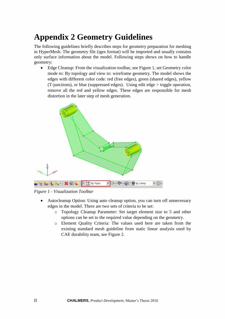
II CHALMERS, Product Development, Master’s Thesis 2016
Appendix 2 Geometry Guidelines The following guidelines briefly describes steps for geometry preparation for meshing
in HyperMesh. The geometry file (iges format) will be imported and usually contains
only surface information about the model. Following steps shows on how to handle
geometry:
Edge Cleanup: From the visualization toolbar, see Figure 1, set Geometry color
mode to: By topology and view to: wireframe geometry. The model shows the
edges with different color code: red (free edges), green (shared edges), yellow
(T-junctions), or blue (suppressed edges). Using edit edge > toggle operation,
remove all the red and yellow edges. These edges are responsible for mesh
distortion in the later step of mesh generation.
Figure 1 - Visualization Toolbar
Autocleanup Option: Using auto cleanup option, you can turn off unnecessary
edges in the model. There are two sets of criteria to be set:
o Topology Cleanup Parameter: Set target element size to 5 and other
options can be set to the required value depending on the geometry.
o Element Quality Criteria: The values used here are taken from the
existing standard mesh guideline from static linear analysis used by
CAE durability team, see Figure 2.

CHALMERS, Product Development, Master’s Thesis 2016 III
Figure 2 - Element Quality Criteria Panel
Although the Autocleanup feature toggles off the edges using the above set
criteria, it may be required to toggle off certain edges manually to make a better
cleanup of the geometry. Look into the model surface and toggle off any close
edges, narrow converging edges, etc. Any protruding small surfaces can be
removed using the surface edit panel. This activity will be based on the
engineer’s judgment. Fewer edges in geometry model will result in a lower
number of control handles generated at the morphing stage.
Convert the surface model into solid model using:
Geometry>Create>Solids>Bounding surface panel. Select the entire surface
and click on create.
Divide design and non-design volumes: Using Solid edit feature, see Figure 3,
the non-design volume parts can be divided from the design volume. Create
separate collector for each part (Bushing, Damper support, etc.) and transfer the
volume to the respective collector.
Figure 3 - Solid edit feature panel
Create material data for the part.
Create property data for design and non-design volume.

IV CHALMERS, Product Development, Master’s Thesis 2016
Assign property data to design and non-design component in the model.

CHALMERS, Product Development, Master’s Thesis 2016 V
Appendix 3 Mesh Guidelines Guidelines for creating a mesh in HyperMesh.
Method 1- Using Volume Tetra: This is one of the simplest method for creating mesh
for solid components. In the Tetramesh panel, see Figure 4, select Volume Tetra:
Set Enclosed Volume and select the solid model.
Set 2D type to Trias
Set 3D type to Tetras
Set Element to Surf/solid comp
Check Use Curvature option and Set Min Elem size to 1, Feature Angle to 30
and Element Size to 5.
Check Cleanup Elements box and click on Mesh button.
Figure 4 - Volume tetra meshing panel
Observe if there are any failed elements generated after meshing. If this occurs, then
undo the mesh generation and go back to geometry and try to toggle off the edges which
resulted into failed mesh. This will be entirely based on complexity of model and
engineer’s judgment. The primary reason for this behavior in mesh generation are extra
or discontinuous edges present in the model. Repeat the above process till the mesh
generated does not have any failed elements.
Next, check the mesh quality, see Figure 5, on how many mesh fails criteria. Press F10
key, a mesh checking tool appears. Select 3-d mesh.
Click on connectivity button to observe if there are any disconnected element
present.
Click on duplicates button to observe if there are any duplicate mesh present.
Set Warpage value to 10 and click the button: Observe if there are any failed
element.
Set aspect value to 8 and click the button: Observe if there are any failed
element.
Figure 5 - Mesh checking panel
If there are few elements, which does not meet these criteria, then the mesh is okay to
proceed. This scattered faulty mesh are difficult to control and moreover for topology
optimization certain level of distorted mesh are allowed. This error can be ignored by
setting control card: PARAM > CHECK NL to NO

VI CHALMERS, Product Development, Master’s Thesis 2016
If there are too many failed elements found at one location, then undo the mesh. Go
back to the geometry and toggle off the edge which causes this. Mesh the model again
and repeat the process until a satisfactory mesh is generated.
Method 2- Using 2D Mesh and Converting into 3D Mesh: In this process, a 2D mesh
is first generated for the given mesh quality. This 2D mesh is then converted into 3D
mesh. This method provide more control on mesh generation and produces a better
mesh than Volume Tetra, and at the same time, this option is more time consuming
compared to volume tetra.
From 2 D panel, see Figure 6, select the Automesh option.
Select the entire surface of the model.
Select the Size and Bias Option
Enter Element Size: 5
Mesh type: Mixed
Choose: Element to Surf Component, Second Order, Keep Connectivity
Map: Check size, skew, link to opposite edges with AR (auto)
Figure 6 - 2D Mesh creation panel
Click on mesh button. To control mesh on surface, option: Mesh Style, biasing
can be explored to control mesh on particular surface. Go to Checks button, set
Warpage value to 10 and observe where the mesh is deforming. Click on create
mesh option.
The mesh generated can be checked by mesh checking tool (F10). Observe how many
2 -D elements failed. If a cluster of failed elements are found at one location, then undo
the mesh, rework on the geometry by using toggle option from edge edit. Once a
satisfactory mesh is obtained, move to the next step.
From 3D panel, see Figure 7, go to Tetra Mesh Panel> Select Tetra Mesh.
Set Fix trias/quads to tetra mesh > Elements > Select the all the 2D Elements
Check fix comp boundaries, update input shells.
Select Create per-volume comps
Click on Mesh.
Figure 7 - 3D Mesh Creation Panel

CHALMERS, Product Development, Master’s Thesis 2016 VII
Check the mesh using the mesh checking tool and verify that the generated mesh are
within the limits, otherwise, reiterate the steps. Now delete the 2D mesh and keep only
3D mesh. Rename the new mesh component generated in the previous step according
to the model.
At this stage, it is recommended to verify whether the generated mesh works or not.
Setup any random fixing constraint and apply random load. Setup the load step for the
load and constraint.
Go to Analysis > OptiStruct > runoption >Check. Click on OptiStruct button and run
the Check Simulation. This command verifies whether the input data mesh is okay or
not. If the software throws an error and rework on meshing and troubleshoot. Remove
the load and constraint from the model.

VIII CHALMERS, Product Development, Master’s Thesis 2016
Appendix 4 Boundary Conditions and
Loading Guidelines The general guideline for setting boundary conditions and loading conditions in
HyperMesh software are as follow:
Create a collector for each RBE (Rigid Body Elements) for the non-design
component.
Create a node at each hard points on the model and move it to the respective
collector.
In the RBE Creation Panel (Figure 8): Go to 1D panel > Rigids > create > Select
the target node (at the hard points node) and select the parent node from the
surface face selection. Follow the guidelines from “fe_procees” for each
individual component on where to setup the rigid connections.
Figure 8 - RBEs creation panel
1. Create collector for SPC and Loads as per the input from load data.
2. Define the constraints at the node and add it to the SPC collector.
3. Define the loads to be applied at the hard points according to the guideline and
add it to the respective collector.
4. Create load step for the model using SPC and Loads defined in the previous
steps for each load case.
5. The FE model is ready and to verify the input data by the “Check” operation in
OptiStruct should be executed.

CHALMERS, Product Development, Master’s Thesis 2016 IX
Appendix 5 Topology and Shape
Optimization Guideline The topology optimization guidelines shows the options present in HyperMesh and the
process to set up the model with optimization settings.
In the Analysis > optimization panel, setup the following:
1. Response setup (Figure 9): Define the response name and select the response
type (mass, static deflection, etc.). For mass response type, select the property
defined by design space. For the displacement response, select the node at the
hard point and select the direction for the response (dof 1, 2, 3 etc.).
Figure 9 - Response setup panel
2. Constraint Setup (Figure 10): Click on the dconstraint button and enter the name
for the constraint. Select the response and set up the upper and lower bound for
the particular hard point depending on the requirement. Select the loadstep for
the constraint.
Figure 10 - Constraint setup panel
3. Objective function (Figure 10): Click on objective button and select the
response to be minimized.
Figure 10 - Objective function setup panel
4. Design variable setup for topology (Figure 11): Click on topology button, enter
design variable name and select the design volume property. Other setting in
the panel can be made depending on the input from manufacturing constraint.
Figure 11 - Topology design variable setup panel

X CHALMERS, Product Development, Master’s Thesis 2016
5. Design variable setup for shape (Figure 12): Click on the shape button. Select
the saved shape from the morphing stage. Enter the upper and lower limit for
the shape (s) as identified in morphing step. Here, multiple shapes can also be
added as shape variables. For creating multiple shape variable, select the option
multiple devsar. Click on create button.
Figure 12 - Shape design variable setup
6. Opti Control Setup (Figure 13) :Click on Opti control button and set the
following value:
a. DESMAX 300
b. OBJTOL 1e-04
c. MATINIT 0.100
d. MINDENS 1e-04
e. OPTMETH MFD
f. DISCRETE Default
Figure 13 - Opti control setup
Note: The value stated above are not standard and are obtained by running multiple
simulations for the sample models.

CHALMERS, Product Development, Master’s Thesis 2016 XI
Appendix 6 Morphing Guideline The morphing guidelines shows the option present in HyperMesh to carry out the
morphing in the models.
7. Morph domain (Figure 14): Define the morphing region using domain by
selecting the design volume region. The morphing domain is very critical to this
process since it defines the extent to which the new shapes to the design volume
can be created and the region where the effect of mesh change will be shared.
Define the morphing region using domain by selecting:
Morphing>Create>Domain. Select 3D domain and pick the elements in the
design volume.
Figure 14 - Morphing domain creation panel
1. Handle creation and management (Figure 15): Depending on the options
selected from software, the handles to move the morph region are automatically
created in the design volume. These handles are present on the edges and on the
places where there is a change in geometry. It is important to check the handles
present and remove the unnecessary handles. It might be required to add certain
handles to make sure the mesh does not deform too much when they are used to
create shape. This step is usually based on engineering judgment and one need
to ready to try different options here.
Figure 15 - Handle creation Panel
2. Creation of new shapes: Depending on the identified high density element
regions, select the handles in the region and translate it in the required direction.
From the Morph panel, select move handle option, see Figure 16. There are
multiple options available to alter the handle movement. Translate the handles
as per the requirement. It is required to find the limitation of morphing in this
step. Try using certain morph distance value and create a shape. If the mesh in
the new shape does not show any error (e.g. folded element that produce
negative Jacobian), then it is good to try a higher value. If the mesh shows an
error for negative Jacobian, then try a lower value. This way, it will be possible
to find the applicable shape distance and then save the newly created shape (as
node perbutation), see Figure 17. The shape created here has upper limit of 1 in
the defined direction. Undo all morph generated in the model.

XII CHALMERS, Product Development, Master’s Thesis 2016
Figure 16 - Move handle panel
Figure 17 - Save shape panel
3. Find the lower limit of shape: Next it is required to find the limitation of the
shape in the opposite direction. In order to find the limitation of the shape, use
apply shape option present in same panel, see Figure 18. Using the apply shape
feature, enter a factor and apply the shape, check if the mesh shows an error. If
the mesh in the new shape does not show any error for folded element, then it
is good to try a higher factor. If the mesh shows an error for folded element,
then try a lower factor. By this step, the engineer will have the knowledge of
the shape, its limitation and the factor with which it can be morphed in the two
direction (positive and negative) representing increase and decrease in design
volume.
Figure 18 - Apply shape panel

CHALMERS, Product Development, Master’s Thesis 2016 XIII
Appendix 7 Post Processing Guidelines This guideline can used for interpreting the result obtained from shape and topology
optimization. Following output files will be required to carry the post processing:
o Filename_des.h3d
o Filename_hist.mvw
o Filename.out
Check Convergence: In order to make sure that the optimization result has been
satisfied all the optimization criteria and has converged, it can be checked by
two ways:
a. Open Filename_hist.mvw file and see the graphs for each criteria
whether it is violated or not.
b. Open the *.out file in the notepad editor and scroll down to the last
iteration. A message will be displayed to indicate whether constraint are
satisfied or violated, see Figure 19.
2. Weight of topology structure: From Filename.out file, note down the final
optimized weight of the geometry as indicated in the last iteration, see Figure
19.
3. Shape design variable limit: From the shape optimization result, the final value
for the design variable limit: upper limit and lower limit will be displayed in
Filename.out file, see Figure 19. This value represents by what factor the shape
actually moved in shape and topology optimization with respect to the defined
shape.
Figure 19 - Sample Filename.out file
4. Run HyperView application and load the model: Filename_des.h3d. Select the
Contour Icon from the menu (Figure 20):

XIV CHALMERS, Product Development, Master’s Thesis 2016
a. Select Result Type as Element Density
b. Averaging method: Simple
Figure 20 - Contour Panel
Click on ISO icon (Figure 21):
c. Select Result Type as Element Density
d. Averaging method: Simple
Figure 21 - Contour ISO view Panel
By dragging the ISO value, you can observe the topology structure in the
component. Also, you can animate the view to observe the topology formation
with each iteration. From this result, the red region represent the high density
element region. Observe the various regions and make a note on where all it is
possible to increase the design volume. Also, the blue region represent low
density elements. These are the regions where it is possible to remove material.
At these region it is possible to reduce the design space. This observations will
be later used in the morphing of the mesh for shape optimization.
5. Run HyperView application and load the model: Filename_des.h3d. Select the
Contour Icon from the menu
a. Select Result Type as Shape Change
b. Direction for shape change
Click on ISO icon:
c. Select Result Type as Shape Change
d. Direction for shape change
Using the above setting, the shape change in the model can be visualized.
6. Export the topology optimized geometry as *.stl file with an iso value at which
the topology seems to be well connected (Tools>Export).