Working Paper/Document de travail 2014-40

Balance Sheets of Financial Intermediaries: Do They Forecast Economic Activity?

by Rodrigo M. Sekkel

2

Bank of Canada Working Paper 2014-40

September 2014

Balance Sheets of Financial Intermediaries: Do They Forecast Economic Activity?

by

Rodrigo M. Sekkel

Canadian Economic Analysis Department Bank of Canada

Ottawa, Ontario, Canada K1A 0G9 rsekkel@bankofcanada.ca

Bank of Canada working papers are theoretical or empirical works-in-progress on subjects in economics and finance. The views expressed in this paper are those of the author.

No responsibility for them should be attributed to the Bank of Canada.

ISSN 1701-9397 © 2014 Bank of Canada

ii

Acknowledgements

I thank Natsuki Arai, Laurence Ball, Jon Faust, Glen Keenleyside, Soojin Jo, Jon Samuels, Hyun Song Shin, Jonathan Wright, Sarah Zubairy and two anonymous referees for useful comments and conversations, as well as comments from participants in the 2013 Latin American Econometric Society Meeting, 2013 Midwest Econometrics Group Meeting, 2013 DIW Macroeconomics Workshop, 2013 IWH/CIREQ Macroeconomics Workshop and the 2014 Society for Nonlinear Dynamics and Econometrics.

iii

Abstract

This paper conducts a real-time, out-of-sample analysis of the forecasting power of various aggregate financial intermediaries’ balance sheets to a wide range of economic activity measures in the United States. I find evidence that the balance sheets of leveraged financial institutions do have out-of-sample predictive power for future economic activity, and this predictability arises mainly through the housing sector. Nevertheless, I show that these variables have very little predictive power during periods of economic expansions and that predictability arises mainly during the financial crisis period.

JEL classification: C53 Bank classification: Econometric and statistical methods

Résumé

Dans cette étude, l’auteur effectue une analyse en temps réel du pouvoir prédictif hors échantillon des données de bilan agrégées de divers intermédiaires financiers relativement à un large éventail de mesures de l’activité économique américaine. Il constate que les bilans des institutions financières à effet de levier permettent de prédire hors échantillon l’évolution future de l’activité économique, et que ce pouvoir se manifeste surtout par le canal du secteur du logement. Néanmoins, il montre que ces variables ont un pouvoir prédictif très faible en période d’expansion économique et que celui-ci apparaît principalement lors de crises financières.

Classification JEL : C53 Classification de la Banque : Méthodes économétriques et statistiques

1 Introduction

The extent of the recent turmoil in financial markets and its long-lasting spillover effects

to the real economy has renewed interest in studies of the interaction between credit conditions

and the macroeconomy. More meaningfully, it has called attention to the role played by

financial intermediaries in the fluctuations of risk premia and economic activity.

This paper conducts a careful examination of the predictive power of different financial

intermediaries’ balance sheets to future changes in a wide set of economic activity measures

in the United States. Unlike previous research, I conduct all my forecasting tests in an

out-of-sample, real-time setting. I report evidence that the balance sheets of some financial

intermediaries, namely security broker-dealers, and, to a lesser extent, shadow banks, have

out-of-sample power in real-time for future economic activity. Nevertheless, I also find that the

informational content of the balance sheets are quite unstable, accruing more significantly in

recessionary periods, and/or times of financial stress. I then show, using data-rich forecasting

methods, that the information contained in these balance sheets is roughly equal to that of

traditional macrofinancial series in normal economic environments.1 On the data front, I

contribute to the real-time forecasting literature by constructing a quarterly real-time data

set of aggregate financial intermediaries’ balance sheets as released quarterly by the Flow of

Funds of the Federal Reserve Board.

My results also point to the relevant channels through which fluctuations in financial

intermediaries’ balance sheets forecast economic growth. I find that the predictive power of

these balance sheets for future GDP arises mainly through the housing sector. Fluctuations in

broker-dealers’ leverage and equity are strong predictors of expected real housing investment

growth. This predictability is to a large extent orthogonal to the information contained in

traditional macro and financial indicators.

Several papers have recently called attention to the importance of financial intermediaries’

balance sheets for the economy. On the theoretical front, a large number of recent papers show

how fluctuations in balance sheets of financial intermediaries impact economic activity and

amplify economic shocks. Meh and Moran (2010), Christensen et al. (2011) and Sandri and

1I define normal economic environments as periods absent of recessions and financial crisis.

2

Valencia (2013) develop dynamic stochastic general-equilibrium (DSGE) models to study how

financial intermediaries’ balance sheets may amplify shocks to the economy, as well as become

the source of economic activity fluctuations themselves, following significant disturbances to

their net worth. These studies generally show that shocks to financial intermediaries’ balance

sheets have a much more disruptive effect on economic activity than shocks to households’

or non-financial firms’ balance sheets. This is mainly due to the higher leverage of financial

intermediaries, which hinders their ability to buffer shocks to their net worth. Thus, an

exogenous shock to financial intermediaries’ net worth leads to a high reduction in their risk-

bearing capacity, resulting in a significant cut in financial intermediation, and hence a fall

in economic activity. By this same mechanism, one would expect that shocks to the highly

leveraged financial intermediaries, such as broker-dealers, have a stronger potential to impact

economic activity than shocks to the commercial banks’ balance sheets.2

On the empirical side, Adrian and Shin (2010a) is one of the first studies to show that

fluctuations in the balance sheets of financial institutions, especially broker-dealers, contain

in-sample forecasting power for future GDP growth. Additionally, Adrian et al. (2010) argue

that the balance sheets of broker-dealers and shadow banks have information for expected

returns of various bond and equity markets in the United States.3 This result holds in- and

out-of-sample, as well as before the financial crisis. Nonetheless, these authors do not study

the out-of-sample predictability of economic activity by means of these financial intermedi-

aries’ balance sheets. Kollmann and Zeugner (2012), on the other hand, show that the leverage

of various sectors of the economy (financial, non-financial firms, and households) has both

in-sample and out-of-sample forecasting power for economic activity. I add to their results

by considering a real-time setting with additional financial intermediaries, more measures

of economic activity, and by conducting a more systematic evaluation of the time-varying

out-of-sample forecasting performance of the different models.

2For a comparison of the balance-sheet dynamics of commercial banks and broker-dealers, see Adrian and Shin(2010b) and Nuno and Thomas (2013).

3Additionally, Adrian et al. (2009) argue that fluctuations in the aggregate balance sheets of broker-dealersforecast exchange rate returns for a large set of countries at weekly, monthly and quarterly horizons, both in- andout-of-sample. Etula (2013) shows that broker-dealers’ asset growth forecasts a wide range of commodity prices atquarterly horizons, both in- and out-of-sample.

3

The paper is organized as follows. Section 2 discusses the data. Section 3 provides an

initial exploration of the forecasting power of balance sheets of financial intermediaries in a

simple set-up. The next section explores how the forecasting power of financial intermediaries’

balance sheets compares to traditional macroeconomic and financial predictors, and examines

its time stability. Section 4 concludes.

2 Data

I use quarterly data of financial intermediaries’ balance sheets, and macroeconomic and fi-

nancial indicators from 1985Q1 to 2010Q4, to study the predictability of a diverse group of

economic activity variables, namely: gross domestic product, industrial production, non-farm

payroll, real private investment, real housing investment, and durable consumption. In this

section, I detail how I constructed my financial intermediaries’ balance sheets, as well as

macrofinancial data set.

In assessing the marginal predictive content of financial variables for real activity using

real-time data, an important issue is that the latter are constantly being revised. I follow

Faust and Wright (2009) and use the data as recorded two quarters after the quarter to which

the data refer as the realized value. For the national income and product accounts data, this

corresponds to the data as recorded in the second revision.

2.1 Financial intermediaries’ balance-sheet data

I investigate the predictive power of aggregate balance-sheet fluctuations of the following

financial intermediaries: (i) commercial banks (CB), comprising commercial banks, credit

unions and savings institutions; (ii) securities broker-dealers (BD); (iii) shadow banks (SB),

comprising issuers of asset-backed securities, finance corporations and funding corporations;

and (iv) agency- and government-sponsored enterprise (GSE)-backed mortgage pools.4 Table

4(i) Commercial banks are financial institutions that raise funds through demand and time deposits as wellas from other sources, such as federal funds purchases and security repurchase agreements, funds from parentcompanies, and borrowing from other lending institutions, and use the funds to make loans, primarily to businessesand individuals, and to invest in securities. (ii) Broker-dealers are financial institutions that buy and sell securitiesfor a fee, hold an inventory of securities for resale, or do both. (iii) Issuers of asset-backed securities (ABS) are

4

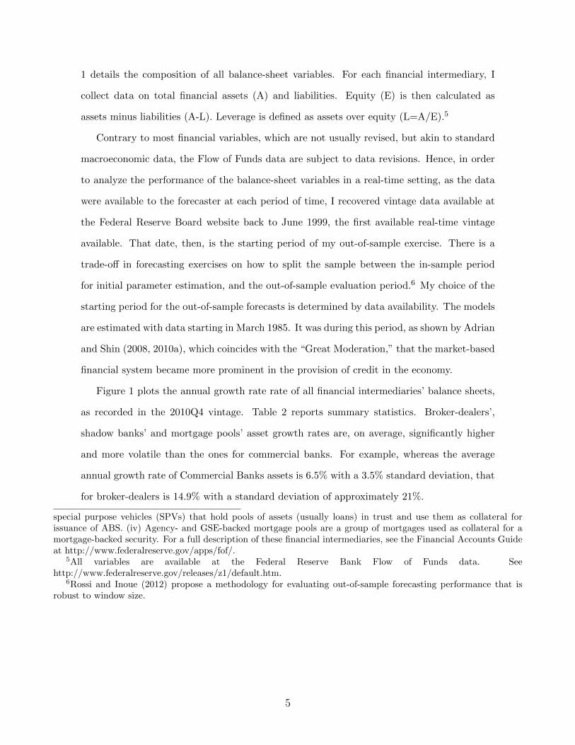
1 details the composition of all balance-sheet variables. For each financial intermediary, I

collect data on total financial assets (A) and liabilities. Equity (E) is then calculated as

assets minus liabilities (A-L). Leverage is defined as assets over equity (L=A/E).5

Contrary to most financial variables, which are not usually revised, but akin to standard

macroeconomic data, the Flow of Funds data are subject to data revisions. Hence, in order

to analyze the performance of the balance-sheet variables in a real-time setting, as the data

were available to the forecaster at each period of time, I recovered vintage data available at

the Federal Reserve Board website back to June 1999, the first available real-time vintage

available. That date, then, is the starting period of my out-of-sample exercise. There is a

trade-off in forecasting exercises on how to split the sample between the in-sample period

for initial parameter estimation, and the out-of-sample evaluation period.6 My choice of the

starting period for the out-of-sample forecasts is determined by data availability. The models

are estimated with data starting in March 1985. It was during this period, as shown by Adrian

and Shin (2008, 2010a), which coincides with the “Great Moderation,” that the market-based

financial system became more prominent in the provision of credit in the economy.

Figure 1 plots the annual growth rate rate of all financial intermediaries’ balance sheets,

as recorded in the 2010Q4 vintage. Table 2 reports summary statistics. Broker-dealers’,

shadow banks’ and mortgage pools’ asset growth rates are, on average, significantly higher

and more volatile than the ones for commercial banks. For example, whereas the average

annual growth rate of Commercial Banks assets is 6.5% with a 3.5% standard deviation, that

for broker-dealers is 14.9% with a standard deviation of approximately 21%.

special purpose vehicles (SPVs) that hold pools of assets (usually loans) in trust and use them as collateral forissuance of ABS. (iv) Agency- and GSE-backed mortgage pools are a group of mortgages used as collateral for amortgage-backed security. For a full description of these financial intermediaries, see the Financial Accounts Guideat http://www.federalreserve.gov/apps/fof/.

5All variables are available at the Federal Reserve Bank Flow of Funds data. Seehttp://www.federalreserve.gov/releases/z1/default.htm.

6Rossi and Inoue (2012) propose a methodology for evaluating out-of-sample forecasting performance that isrobust to window size.

5

2.2 Macroeconomic and financial series

In order to compare the predictability provided by the aggregate financial intermediaries’

balance-sheet variables to more traditional predictors, I construct a panel of commonly used

macroeconomic and financial predictors of economic activity. Since I estimate the models with

only real-time data, the panel is composed of significantly more financial than macroeconomic

series: the number of potential financial predictors (which are not revised) is higher than the

number of commonly available real-time macroeconomic series. All macro series were obtained

with the Federal Reserve Bank of Philadelphia Real-Time Dataset for Macroeconomists. All

the financial series refer to the last day of the second month of each quarter. Table 3 lists the

data used, as well as the transformation applied to each series in order to ensure stationarity.

In total, I use 15 macroeconomic series, 60 financial predictors and 8 different balance-sheet

measures from 4 different financial intermediaries’ sectors.

3 Forecasting models

I start by examining whether simple predictive regressions augmented with balance-sheet

variables provide more accurate forecasts than the simple autoregressive model.

Let yt be the annualized growth rate from t-1 to t of the variable to be forecasted, and

xit the n × 1 predictor vector. yt+h is the h-step-ahead value of the cumulative growth

rate to be forecasted, yt+h =∑h

i=0 yt+i/h. I estimate the following model for each financial

intermediary’s balance-sheet variable separately:

yt+h = α+P∑

j=1

βiyt−j + γxi,t + εt+h, (1)

where yt is the economic activity being forecasted; xi,t is the additional balance-sheet variable

in question. The horizon of the forecast is defined by h. I estimate the above models for h =

0, 1, 2, 3 and 4 quarters ahead. The lag order P of the autoregressive term is defined by the

Bayesian information criterion (BIC).

In order to evaluate the forecasts, I initially report the root mean squared prediction error

6

(RMSPE), defined as

RMSEh =

√√√√ 1

T

T∑t=1

(yt+h − y∗t+h),

where yt+h is the forecast, y∗t+h is the variable as observed two quarters after the quarter to

which the data refer, and T is the number of out-of-sample forecasts.

In order to test whether the ratios of the RMSPEs are different from unity when compar-

ing the financial intermediaries’ balance-sheet forecasts to the benchmark autoregressive (AR)

model, I use the Diebold and Mariano (1995) equal predictive accuracy test. It is known that

when forecasting models are nested, and hence equal in population under the null hypothesis,

the Diebold-Mariano test statistic has a non-standard asymptotic distribution. Clark and

McCracken (2001) and McCracken (2007) provide additional tests to compare nested mod-

els. Nevertheless, Clark and McCracken (2013) show that, in finite samples, the traditional

Diebold-Mariano test statistic provides a good-sized test, even in the case of nested models,

when the correction suggested by Harvey et al. (1997) is used. This approach to inference is

also followed by Faust and Wright (2013) when forecasting inflation.

Table 4 shows the results of these initial forecasts. Mixed results are found for the various

balance-sheet variables. I find evidence that balance-sheet measures associated with security

broker-dealers have a significant forecasting power for some of the economic activity indica-

tors. There is no evidence that commercial banks’ balance sheets provide any information

for forecasting the economic indicators examined here. The inclusion of commercial banks’

and mortgage pools’ balance sheets most often leads to higher RMSPE than the ones from

the benchmark AR models, though this is often not significant, especially for mortgage pools.

This result is consistent with previous findings by Adrian et al. (2010), who find that the

informational content of balance-sheet variables for economic activity and risk premia in eq-

uity and bond markets is mainly concentrated in the highly leveraged broker-dealers financial

intermediaries.

Among the different broker-dealers’ balance-sheet variables (asset, leverage and equity

growth), it is also noteworthy that measures of equity and leverage are significantly more

7

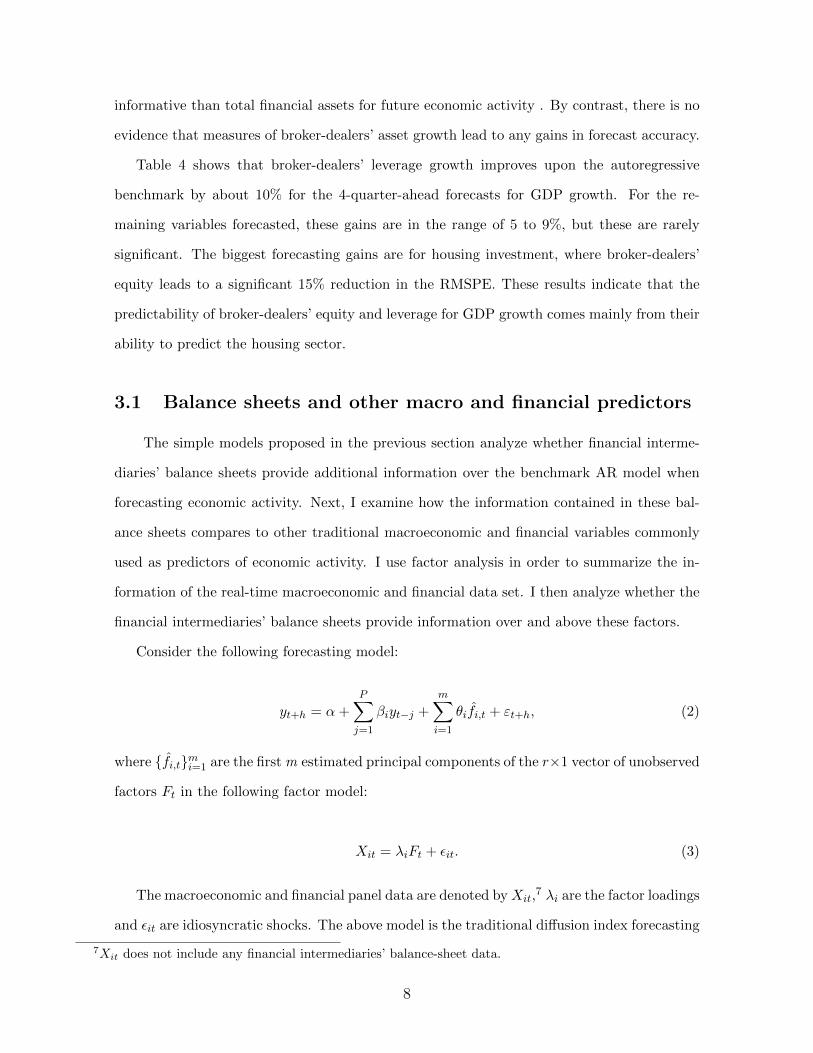
informative than total financial assets for future economic activity . By contrast, there is no

evidence that measures of broker-dealers’ asset growth lead to any gains in forecast accuracy.

Table 4 shows that broker-dealers’ leverage growth improves upon the autoregressive

benchmark by about 10% for the 4-quarter-ahead forecasts for GDP growth. For the re-

maining variables forecasted, these gains are in the range of 5 to 9%, but these are rarely

significant. The biggest forecasting gains are for housing investment, where broker-dealers’

equity leads to a significant 15% reduction in the RMSPE. These results indicate that the

predictability of broker-dealers’ equity and leverage for GDP growth comes mainly from their

ability to predict the housing sector.

3.1 Balance sheets and other macro and financial predictors

The simple models proposed in the previous section analyze whether financial interme-

diaries’ balance sheets provide additional information over the benchmark AR model when

forecasting economic activity. Next, I examine how the information contained in these bal-

ance sheets compares to other traditional macroeconomic and financial variables commonly

used as predictors of economic activity. I use factor analysis in order to summarize the in-

formation of the real-time macroeconomic and financial data set. I then analyze whether the

financial intermediaries’ balance sheets provide information over and above these factors.

Consider the following forecasting model:

yt+h = α+

P∑j=1

βiyt−j +

m∑i=1

θifi,t + εt+h, (2)

where {fi,t}mi=1 are the first m estimated principal components of the r×1 vector of unobserved

factors Ft in the following factor model:

Xit = λiFt + εit. (3)

The macroeconomic and financial panel data are denoted byXit,7 λi are the factor loadings

and εit are idiosyncratic shocks. The above model is the traditional diffusion index forecasting

7Xit does not include any financial intermediaries’ balance-sheet data.

8

framework of Stock and Watson (2002). In order to generate forecasts with diffusion indices,

one needs to choose the number of factors to be included in the forecasting regression. For

the sake of parsimony, I restrict myself to forecasting regressions with the first three factors

F1:3,t.

I first examine how forecasting regressions augmented with the macrofinancial factors, as

in equation (2), and estimated with my real-time data set, compare with the benchmark AR

model. Table 5 shows the results for this comparison. As in Bernanke and Boivin (2003)

and Faust and Wright (2009), I find no gains in forecast accuracy over the benchmark AR

model for the factor-augmented forecasts. As shown by these papers, the real-time nature

of the data is not responsible for the factor model’s poor results. The fact that my panel is

relatively small compared to the data sets traditionally used for factor analysis, as well as the

fact that it significantly overrepresents financial data to the detriment of other macroeconomic

indicators, might explain the factor forecasts’ overall poor results.

Next, I examine how the forecasts generated by the financial intermediaries’ balance-

sheet models as in equation (1) compare with the macrofinancial factors in equation (2).

Table 6 summarizes the results. I find similar improvements over the factor forecasts as for

the benchmark AR models. Nevertheless, most of these improvements are not statistically

significant. A notable exception is again the housing sector, where the gains from forecasting

with broker-dealers’ and shadow banks’ balance sheets at longer horizons are also large and

significant. As in the previous subsection, I find that the forecasting power of financial inter-

mediaries’ balance sheets is concentrated in the sectors most sensitive to credit conditions,

such as housing and durable goods consumption.

3.2 When do (not) financial intermediaries’ balance sheets

add information?

In the previous section, I showed that models augmented with broker-dealers’ leverage

and equity growth, as well as shadow banks’ asset growth, provide significant forecasting

power beyond that already contained in traditional macroeconomic and financial series for

9

future economic activity. Nevertheless, forecasting regressions have recently been shown to

suffer from significant instabilities, as highlighted by Giacomini and Rossi (2010). Hence, one

could envision a situation where forecasting models augmented with financial intermediaries’

balance-sheet variables provide more forecasting power during certain times, such as in periods

marked by financial volatility, than in periods characterized by financial tranquility.

3.2.1 Evidence from Giacomini and Rossi (2010) fluctuation tests

In order to capture the time variation in the relative forecasting performance of these

financial intermediaries’ balance sheets, I apply Giacomini and Rossi (2010) fluctuation tests

for forecast comparisons in unstable environments. Rossi and Sekhposyan (2010) apply the

fluctuation tests to a wide range of models for predicting U.S. GDP growth and inflation.

They find that most of the predictors either completely lost or had their predictive ability

strongly diminished after the mid-1970s.

The focus of Giacomini and Rossi (2010) is the local relative predictive ability of two

competing forecasting models:

rMSFEt =1

m

( t+m/2∑j=t−m/2

ε2t+h −t+m/2∑

j=t−m/2

η2t+h

), (4)

where εt and ηt are the out-of-sample forecast errors of the first (balance sheet) and second

(AR) models, respectively. I construct rolling estimates of the relative mean square forecast

errors (rMSFE) using a two-sided window (m) of 20 quarters to depict the time variation in

the performance of the financial intermediaries’ balance-sheet models relative to that of the

simple AR model.8

The fluctuation tests are based on the following rescaled version of the rMSFE statistic:

FOOSt,m = σ−1m−1/2

( t+m/2∑j=t−m/2

ε2t+h −t+m/2∑

j=t−m/2

η2t+h

), (5)

where σ2 is a heteroscedasticity and autocorrelation consistent estimator of the variance σ2.

The null hypothesis of the tests is that the forecasting performance of both models is

8In the appendix, I test the robustness of the results to different window sizes.

10

equal at each period,

H0 : E(ε2t − η2t ) = 0. (6)

Giacomini and Rossi (2010) show how to approximate the distribution of the fluctuation

tests by functionals of Brownian motions and provide critical values for different significance

levels and window and sample sizes.

Figures 2 to 7 plot the results of the tests, as well as their 10% critical values. Each

figure shows the results for tests conducted with regressions using one financial intermediary’s

balance-sheet variable at a time, as in equation (1). By plotting the time variation in the

FOOSt,m statistic together with the critical values, one can easily see the periods of time when the

statistic crosses the critical values, signalling that the financial intermediaries’ balance-sheet

models outperformed, or were outperformed by, the simple AR benchmark.

It is clear from the figures that balance sheets from commercial banks and mortgage

pools have no forecasting power throughout the whole forecasting sample. For many of the

indicators, models including commercial banks’ leverage and equity produce forecasts that

are actually statistically inferior to the benchmark AR from 2005 to early 2007.

The figures also show that there is a substantial time variation in the forecasting per-

formance of broker-dealers’ equity and leverage growth for economic activity. Whereas fluc-

tuation tests indicate that their forecasting performance was no better than the benchmark

AR model in the first part of the sample, they also show a significant increase in forecasting

power during the last financial crisis and following great recession.

It is also interesting to note that broker-dealers’ equity and leverage growth not only

have a higher forecasting power for housing investment, but that this forecasting power also

arises significantly earlier than for other predicted variables. The fluctuation test signals the

superiority of the broker-dealers’ equity growth model over the benchmark AR as early as

the first semester of 2007.

11

3.3 Real-time vs. revised data

In order to clarify the importance of real-time data for the balance sheet of the financial

intermediaries, this section contrasts the results obtained with real-time data and the ones

estimated with the revised data of balance sheets and macroeconomic aggregates, as they

were observed in the last quarter of 2010.

Results are shown in Table 7. There is little difference in the RMSPE ratios estimated with

fully revised data, as in Bernanke and Boivin (2003) and Faust and Wright (2009). In most

cases, the financial intermediaries’ balance sheet-models with revised data compare slightly

worse with the benchmark AR models than in the fully real-time case. Nevertheless, the

conclusion that broker-dealers’ equity and leverage growth are the most informative predictors

of future economic activity is robust to the use of real-time or revised data.

4 Conclusion

This paper has conducted a time-varying, out-of-sample, real-time analysis of the predic-

tive power of various aggregate financial intermediaries’ balance sheets for a range of economic

activity indicators in the United States. I find that significant forecasting power is restricted

to balance sheets from the more leveraged financial sector, namely broker-dealers. I also show

that there are significant forecasting instabilities in the performance of balance-sheet models.

Through Giacomini and Rossi (2010) fluctuation tests, I find that the positive performance

of broker-dealers’ balance-sheet forecasting models occurs mainly during the crisis period.

12

References

Adrian, T., E. Etula, and H. S. Shin (2009): “Risk appetite and exchange rates,” Federal

Reserve Bank of New York Staff Report, 361.

Adrian, T., E. Moench, and H. S. Shin (2010): “Financial intermediation, asset prices,

and macroeconomic dynamics,” Federal Reserve Bank of New York Staff Report, 422.

Adrian, T. and H. Shin (2008): “Financial Intermediaries, Financial Stability, and Mone-

tary Policy,” Staff Report, Federal Reserve Bank of New York.

Adrian, T. and H. S. Shin (2010a): “Chapter 12 - Financial Intermediaries and Monetary

Economics,” in Handbook of Monetary Economics, ed. by B. Friedman and M. Woodford,

Elsevier, vol. 3 of Handbook of Monetary Economics, 601 – 650.

——— (2010b): “Liquidity and leverage,” Journal of Financial Intermediation, 19, 418–437.

Bernanke, B. and J. Boivin (2003): “Monetary policy in a data-rich environment,” Jour-

nal of Monetary Economics, 50, 525–546.

Christensen, I., C. Meh, and K. Moran (2011): “Bank leverage regulation and macroe-

conomic dynamics,” Bank of Canada Working Paper 2011-32.

Clark, T. and M. McCracken (2001): “Tests of equal forecast accuracy and encompass-

ing for nested models,” Journal of Econometrics, 105, 85–110.

——— (2013): “Chapter 20 - Advances in Forecast Evaluation,” in Handbook of Economic

Forecasting, ed. by G. Elliott and A. Timmermann, Elsevier, vol. 2, Part B of Handbook of

Economic Forecasting, 1107–1201.

Diebold, F. and R. Mariano (1995): “Comparing predictive accuracy,” Journal of Busi-

ness and Economic Statistics, 13, 253–263.

Etula, E. (2013): “Broker-dealer risk appetite and commodity returns,” Journal of Finan-

cial Econometrics, 11, 486–521.

13

Faust, J. and J. H. Wright (2009): “Comparing Greenbook and reduced form forecasts

using a large realtime dataset,” Journal of Business & Economic Statistics, 27, 468–479.

——— (2013): “Chapter 1 - Forecasting Inflation,” in Handbook of Economic Forecasting,

ed. by G. Elliott and A. Timmermann, Elsevier, vol. 2, Part A of Handbook of Economic

Forecasting, 2–56.

Giacomini, R. and B. Rossi (2010): “Forecast comparisons in unstable environments,”

Journal of Applied Econometrics, 25, 595–620.

Harvey, D., S. Leybourne, and P. Newbold (1997): “Testing the equality of prediction

mean squared errors,” International Journal of Forecasting, 13, 281–291.

Kollmann, R. and S. Zeugner (2012): “Leverage as a predictor for real activity and

volatility,” Journal of Economic Dynamics and Control, 36, 1267–1283.

McCracken, M. (2007): “Asymptotics for out of sample tests of Granger causality,” Journal

of Econometrics, 140, 719–752.

Meh, C. and K. Moran (2010): “The role of bank capital in the propagation of shocks,”

Journal of Economic Dynamics and Control, 34, 555–576.

Nuno, G. and C. Thomas (2013): “Bank leverage cycles,” European Central Bank Working

Paper 1524.

Rossi, B. and A. Inoue (2012): “Out-of-sample forecast tests robust to the choice of

window size,” Journal of Business & Economic Statistics, 30, 432–453.

Rossi, B. and T. Sekhposyan (2010): “Have economic models’ forecasting performance

for US output growth and inflation changed over time, and when?” International Journal

of Forecasting, 26, 808–835.

Sandri, D. and F. Valencia (2013): “Financial Crises and Recapitalizations,” Journal of

Money, Credit and Banking, 45, 59–86.

14

Stock, J. and M. Watson (2002): “Forecasting using principal components from a large

number of predictors,” Journal of the American Statistical Association, 97, 1167–1179.

15

Table 1: Composition of Balance-Sheet Variables

Financial Intermediaries Variables

Broker-Dealers (BD) Broker-Dealers

Commercial Banks (CB) Commercial BanksSavings InstitutionsCredit Unions

Shadow Banks (SB) Asset-Backed Securities IssuersFinance CorporationsFunding Corporations

Mortgage Pools (MP) Mortgage Pools

Note: This table shows the composition of all balance-sheet indicators used in the analysis. All data were gath-ered from the Federal Reserve Board Flow of Funds data. Equity is defined as total financial assets minus totalfinancial liabilities, (A− L). Leverage is defined as total financial assets over equity, A/E = A/(A− L).

Table 2: Summary Statistics of Balance-Sheet Explanatory Variables

BDA BDL BDE CBA CBL CBE SBA MPA

Mean 14.86 7.91 11.26 6.58 -3.77 14.30 12.37 10.20Median 15.29 8.61 8.68 7.29 -1.97 10.08 13.09 10.18SD 20.93 29.02 23.35 3.54 16.04 22.90 9.18 17.87Min -40.65 -64.67 -37.30 -1.94 -46.74 -30.27 -21.42 -80.03Max 97.45 100.04 94.31 14.14 46.00 107.83 37.20 45.83AR(1) 0.75 0.72 0.71 0.91 0.73 0.74 0.99 0.99

Note: The balance-sheet sample is quarterly and goes from 1985Q1 to 2010Q4 as recorded in the 2010Q4vintage. All data refer to annual growth rates in percentage points. BDA: Broker-Dealers Asset, BDL:Broker-Dealers Leverage, BDE: Broker-Dealers Equity, CBA: Commercial Banks Asset, CBL: CommercialBanks Leverage, CBE: Commercial Banks Equity, SBA: Shadow Banks Asset, MPA: Mortgage Pools Asset.

16

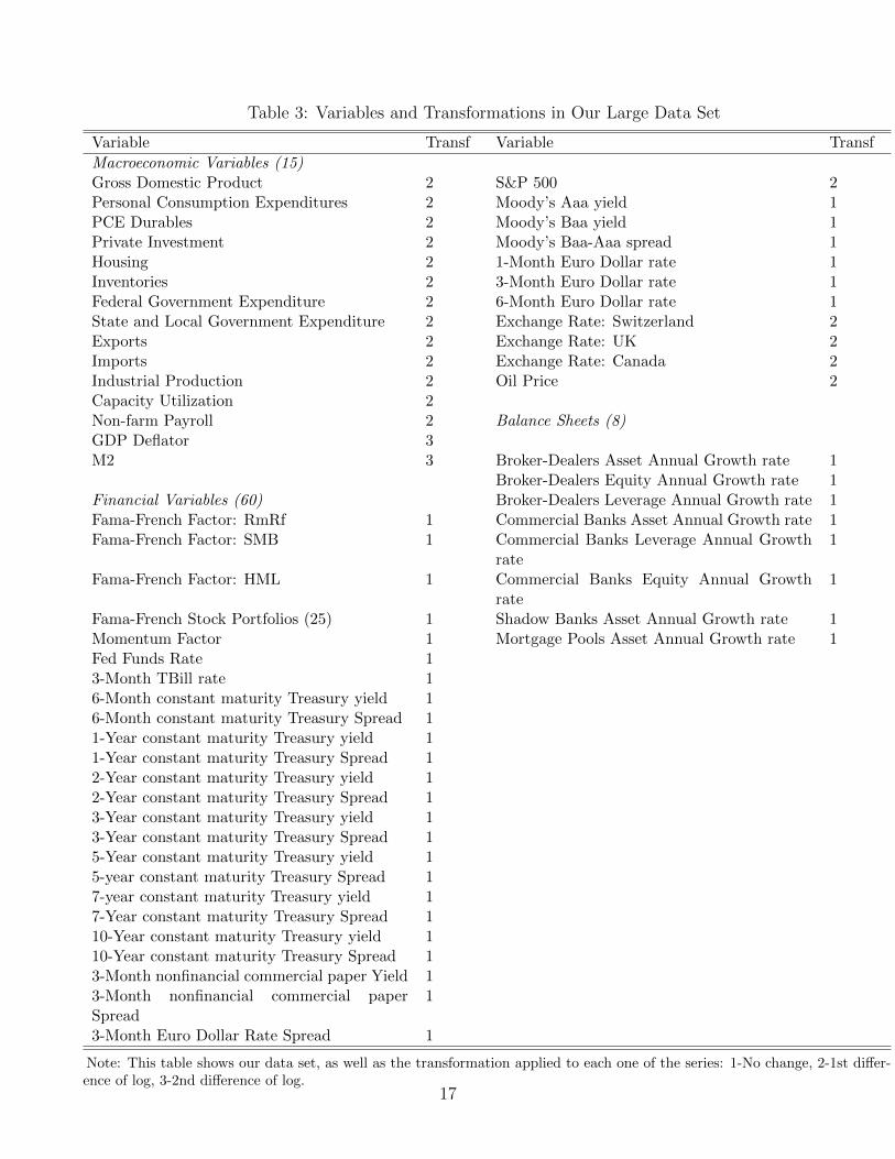
Table 3: Variables and Transformations in Our Large Data Set

Variable Transf Variable Transf

Macroeconomic Variables (15)Gross Domestic Product 2 S&P 500 2Personal Consumption Expenditures 2 Moody’s Aaa yield 1PCE Durables 2 Moody’s Baa yield 1Private Investment 2 Moody’s Baa-Aaa spread 1Housing 2 1-Month Euro Dollar rate 1Inventories 2 3-Month Euro Dollar rate 1Federal Government Expenditure 2 6-Month Euro Dollar rate 1State and Local Government Expenditure 2 Exchange Rate: Switzerland 2Exports 2 Exchange Rate: UK 2Imports 2 Exchange Rate: Canada 2Industrial Production 2 Oil Price 2Capacity Utilization 2Non-farm Payroll 2 Balance Sheets (8)GDP Deflator 3M2 3 Broker-Dealers Asset Annual Growth rate 1

Broker-Dealers Equity Annual Growth rate 1Financial Variables (60) Broker-Dealers Leverage Annual Growth rate 1Fama-French Factor: RmRf 1 Commercial Banks Asset Annual Growth rate 1Fama-French Factor: SMB 1 Commercial Banks Leverage Annual Growth

rate1

Fama-French Factor: HML 1 Commercial Banks Equity Annual Growthrate

1

Fama-French Stock Portfolios (25) 1 Shadow Banks Asset Annual Growth rate 1Momentum Factor 1 Mortgage Pools Asset Annual Growth rate 1Fed Funds Rate 13-Month TBill rate 16-Month constant maturity Treasury yield 16-Month constant maturity Treasury Spread 11-Year constant maturity Treasury yield 11-Year constant maturity Treasury Spread 12-Year constant maturity Treasury yield 12-Year constant maturity Treasury Spread 13-Year constant maturity Treasury yield 13-Year constant maturity Treasury Spread 15-Year constant maturity Treasury yield 15-year constant maturity Treasury Spread 17-year constant maturity Treasury yield 17-Year constant maturity Treasury Spread 110-Year constant maturity Treasury yield 110-Year constant maturity Treasury Spread 13-Month nonfinancial commercial paper Yield 13-Month nonfinancial commercial paperSpread

1

3-Month Euro Dollar Rate Spread 1

Note: This table shows our data set, as well as the transformation applied to each one of the series: 1-No change, 2-1st differ-ence of log, 3-2nd difference of log.

17

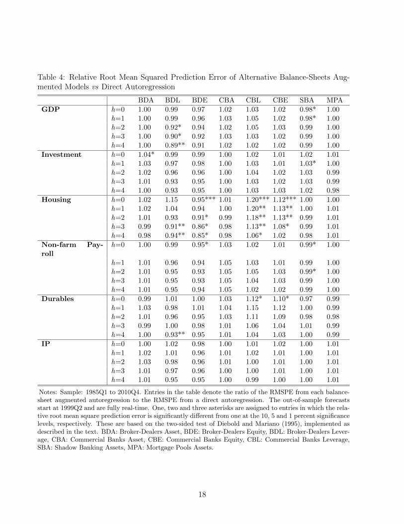
Table 4: Relative Root Mean Squared Prediction Error of Alternative Balance-Sheets Aug-mented Models vs Direct Autoregression

BDA BDL BDE CBA CBL CBE SBA MPA

GDP h=0 1.00 0.99 0.97 1.02 1.03 1.02 0.98* 1.00h=1 1.00 0.99 0.96 1.03 1.05 1.02 0.98* 1.00h=2 1.00 0.92* 0.94 1.02 1.05 1.03 0.99 1.00h=3 1.00 0.90* 0.92 1.03 1.03 1.02 0.99 1.00h=4 1.00 0.89** 0.91 1.02 1.02 1.02 0.99 1.00

Investment h=0 1.04* 0.99 0.99 1.00 1.02 1.01 1.02 1.01h=1 1.03 0.97 0.98 1.00 1.03 1.01 1.03* 1.00h=2 1.02 0.96 0.96 1.00 1.04 1.02 1.03 0.99h=3 1.01 0.93 0.95 1.00 1.03 1.02 1.03 0.99h=4 1.00 0.93 0.95 1.00 1.03 1.03 1.02 0.98

Housing h=0 1.02 1.15 0.95*** 1.01 1.20*** 1.12*** 1.00 1.00h=1 1.02 1.04 0.94 1.00 1.20** 1.13** 1.00 1.01h=2 1.01 0.93 0.91* 0.99 1.18** 1.13** 0.99 1.01h=3 0.99 0.91** 0.86* 0.98 1.13** 1.08* 0.99 1.01h=4 0.98 0.94** 0.85* 0.98 1.06* 1.02 0.98 1.01

Non-farm Pay-roll

h=0 1.00 0.99 0.95* 1.03 1.02 1.01 0.99* 1.00

h=1 1.01 0.96 0.94 1.05 1.03 1.01 0.99 1.00h=2 1.01 0.95 0.93 1.05 1.05 1.03 0.99* 1.00h=3 1.01 0.95 0.93 1.05 1.04 1.03 0.99 1.00h=4 1.01 0.95 0.94 1.05 1.02 1.02 0.99 1.00

Durables h=0 0.99 1.01 1.00 1.03 1.12* 1.10* 0.97 0.99h=1 1.03 0.98 1.01 1.04 1.15 1.12 1.00 0.99h=2 1.01 0.96 0.95 1.03 1.11 1.09 0.98 0.98h=3 0.99 1.00 0.98 1.01 1.06 1.04 1.01 0.99h=4 1.00 0.93** 0.95 1.01 1.04 1.03 1.00 0.99

IP h=0 1.00 1.02 0.98 1.00 1.01 1.02 1.00 1.01h=1 1.02 1.01 0.96 1.01 1.02 1.01 1.00 1.01h=2 1.03 0.98 0.96 1.01 1.00 1.01 1.00 1.01h=3 1.01 0.97 0.96 1.00 1.00 1.01 1.00 1.01h=4 1.01 0.95 0.95 1.00 0.99 1.00 1.00 1.01

Notes: Sample: 1985Q1 to 2010Q4. Entries in the table denote the ratio of the RMSPE from each balance-sheet augmented autoregression to the RMSPE from a direct autoregression. The out-of-sample forecastsstart at 1999Q2 and are fully real-time. One, two and three asterisks are assigned to entries in which the rela-tive root mean square prediction error is significantly different from one at the 10, 5 and 1 percent significancelevels, respectively. These are based on the two-sided test of Diebold and Mariano (1995), implemented asdescribed in the text. BDA: Broker-Dealers Asset, BDE: Broker-Dealers Equity, BDL: Broker-Dealers Lever-age, CBA: Commercial Banks Asset, CBE: Commercial Banks Equity, CBL: Commercial Banks Leverage,SBA: Shadow Banking Assets, MPA: Mortgage Pools Assets.

18

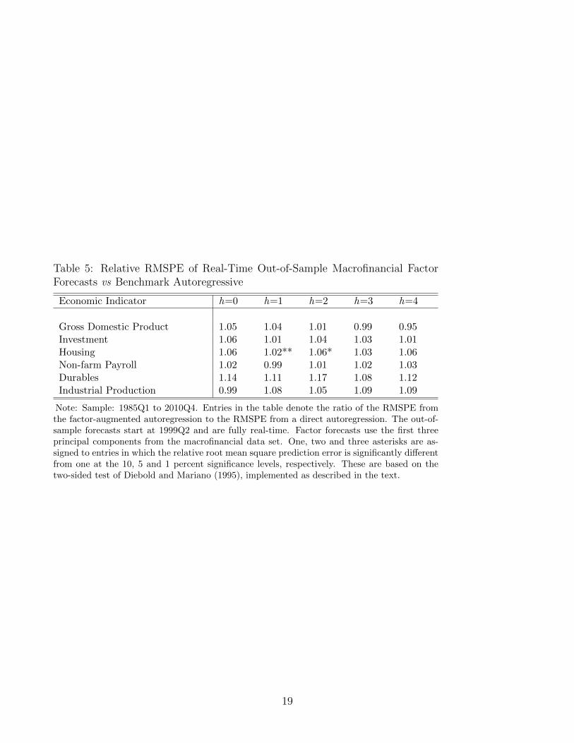
Table 5: Relative RMSPE of Real-Time Out-of-Sample Macrofinancial FactorForecasts vs Benchmark Autoregressive

Economic Indicator h=0 h=1 h=2 h=3 h=4

Gross Domestic Product 1.05 1.04 1.01 0.99 0.95Investment 1.06 1.01 1.04 1.03 1.01Housing 1.06 1.02** 1.06* 1.03 1.06Non-farm Payroll 1.02 0.99 1.01 1.02 1.03Durables 1.14 1.11 1.17 1.08 1.12Industrial Production 0.99 1.08 1.05 1.09 1.09

Note: Sample: 1985Q1 to 2010Q4. Entries in the table denote the ratio of the RMSPE fromthe factor-augmented autoregression to the RMSPE from a direct autoregression. The out-of-sample forecasts start at 1999Q2 and are fully real-time. Factor forecasts use the first threeprincipal components from the macrofinancial data set. One, two and three asterisks are as-signed to entries in which the relative root mean square prediction error is significantly differentfrom one at the 10, 5 and 1 percent significance levels, respectively. These are based on thetwo-sided test of Diebold and Mariano (1995), implemented as described in the text.

19

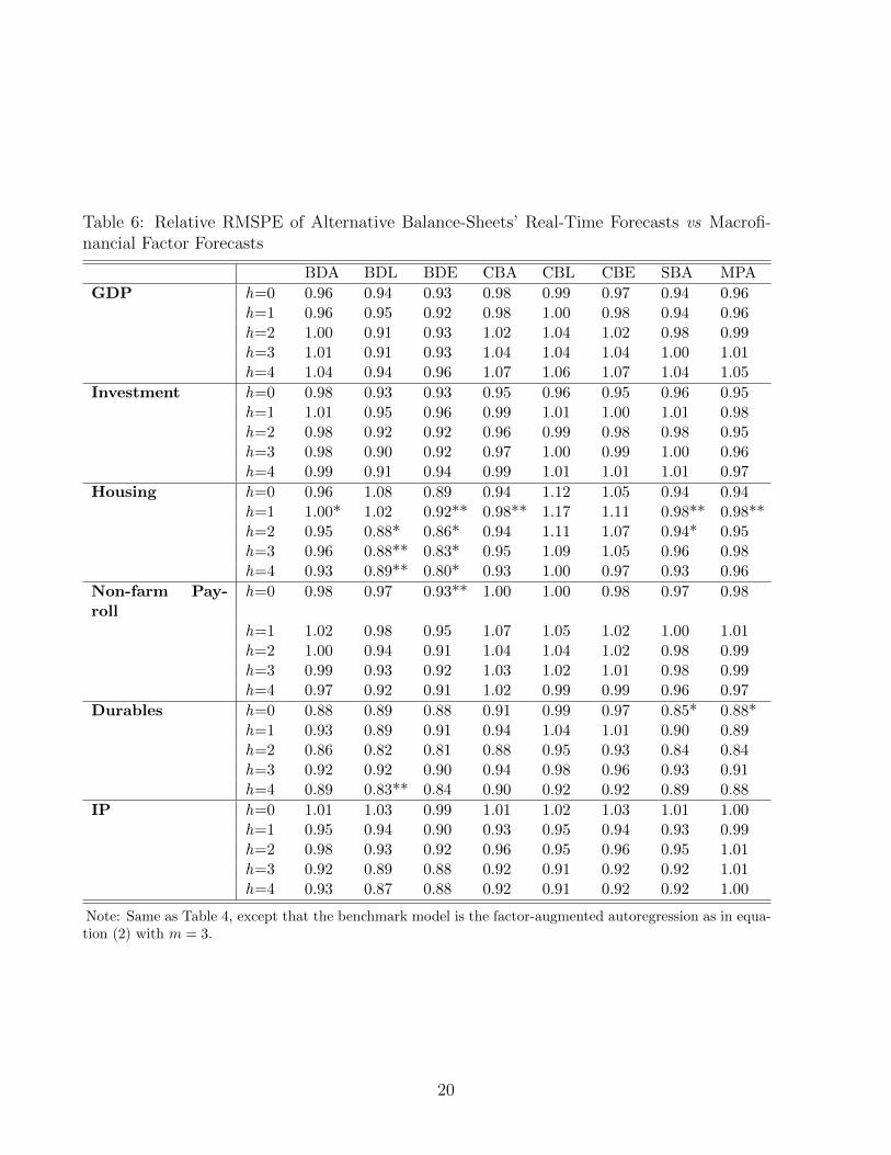
Table 6: Relative RMSPE of Alternative Balance-Sheets’ Real-Time Forecasts vs Macrofi-nancial Factor Forecasts

BDA BDL BDE CBA CBL CBE SBA MPA

GDP h=0 0.96 0.94 0.93 0.98 0.99 0.97 0.94 0.96h=1 0.96 0.95 0.92 0.98 1.00 0.98 0.94 0.96h=2 1.00 0.91 0.93 1.02 1.04 1.02 0.98 0.99h=3 1.01 0.91 0.93 1.04 1.04 1.04 1.00 1.01h=4 1.04 0.94 0.96 1.07 1.06 1.07 1.04 1.05

Investment h=0 0.98 0.93 0.93 0.95 0.96 0.95 0.96 0.95h=1 1.01 0.95 0.96 0.99 1.01 1.00 1.01 0.98h=2 0.98 0.92 0.92 0.96 0.99 0.98 0.98 0.95h=3 0.98 0.90 0.92 0.97 1.00 0.99 1.00 0.96h=4 0.99 0.91 0.94 0.99 1.01 1.01 1.01 0.97

Housing h=0 0.96 1.08 0.89 0.94 1.12 1.05 0.94 0.94h=1 1.00* 1.02 0.92** 0.98** 1.17 1.11 0.98** 0.98**h=2 0.95 0.88* 0.86* 0.94 1.11 1.07 0.94* 0.95h=3 0.96 0.88** 0.83* 0.95 1.09 1.05 0.96 0.98h=4 0.93 0.89** 0.80* 0.93 1.00 0.97 0.93 0.96

Non-farm Pay-roll

h=0 0.98 0.97 0.93** 1.00 1.00 0.98 0.97 0.98

h=1 1.02 0.98 0.95 1.07 1.05 1.02 1.00 1.01h=2 1.00 0.94 0.91 1.04 1.04 1.02 0.98 0.99h=3 0.99 0.93 0.92 1.03 1.02 1.01 0.98 0.99h=4 0.97 0.92 0.91 1.02 0.99 0.99 0.96 0.97

Durables h=0 0.88 0.89 0.88 0.91 0.99 0.97 0.85* 0.88*h=1 0.93 0.89 0.91 0.94 1.04 1.01 0.90 0.89h=2 0.86 0.82 0.81 0.88 0.95 0.93 0.84 0.84h=3 0.92 0.92 0.90 0.94 0.98 0.96 0.93 0.91h=4 0.89 0.83** 0.84 0.90 0.92 0.92 0.89 0.88

IP h=0 1.01 1.03 0.99 1.01 1.02 1.03 1.01 1.00h=1 0.95 0.94 0.90 0.93 0.95 0.94 0.93 0.99h=2 0.98 0.93 0.92 0.96 0.95 0.96 0.95 1.01h=3 0.92 0.89 0.88 0.92 0.91 0.92 0.92 1.01h=4 0.93 0.87 0.88 0.92 0.91 0.92 0.92 1.00

Note: Same as Table 4, except that the benchmark model is the factor-augmented autoregression as in equa-tion (2) with m = 3.

20

Table 7: Relative Root Mean Square Error of Alternative Balance Sheets over BenchmarkAutoregressive - Final Revised Data

BDA BDL BDE CBA CBL CBE SBA MPA

GDP h=0 1.00 1.00 0.98 1.02 1.02 1.03 0.98* 1.00h=1 1.00 0.99 0.97 1.04 1.04 1.05 0.98 1.00h=2 1.01 0.97 0.94 1.05 1.05 1.06 0.98 1.00h=3 1.00 0.95* 0.93 1.04 1.05 1.05 0.99 1.00h=4 1.00 0.94* 0.93* 1.03 1.04 1.04 0.99 1.00

Investment h=0 1.04 1.00 1.01 1.00 1.01 1.02 1.02* 1.01h=1 1.03 0.98*** 1.00 1.00 1.02 1.03 1.03* 1.00h=2 1.02 0.97** 0.98 1.00 1.03 1.04 1.03* 1.00h=3 1.01 0.96** 0.96 0.99 1.04 1.05 1.03 1.00h=4 1.01 0.95** 0.95 0.99 1.05 1.06 1.03 0.98

Housing h=0 1.03 1.00 0.98 1.00 1.14*** 1.16* 1.00 1.01h=1 1.02 0.98 0.97 1.00 1.12* 1.14 1.00 1.01h=2 1.01 0.96 0.96 1.00 1.11** 1.13 0.99 1.01h=3 0.99 0.93* 0.95 0.99 1.10*** 1.11 0.99 1.01h=4 0.98 0.93* 0.97 0.99 1.07*** 1.08 0.98 1.01

Non-farm Pay-roll

h=0 1.00 1.00 0.96* 1.03 1.03 1.07 1.00 1.00

h=1 1.01 0.98 0.94 1.05 1.07 1.11 0.99 1.00h=2 1.01 0.96 0.92* 1.04 1.07 1.11 0.99 1.00h=3 1.01 0.95 0.92* 1.04 1.08 1.11 0.99 1.00h=4 1.01 0.94 0.92* 1.04 1.07 1.11 0.99 1.00

Durables h=0 0.98 1.01 0.99 1.03 1.05 1.07 0.96 1.00h=1 1.01 0.99 0.97 1.05 1.06 1.09 0.99 0.99h=2 1.00 0.98 0.96 1.03 1.06 1.09 0.97 0.99h=3 1.00 0.98 0.97 1.02 1.06 1.09 1.00 0.99h=4 1.00 0.97 0.95 1.01 1.03 1.06 1.00 1.00

IP h=0 1.00 1.01 1.00 0.99 1.01 1.02 0.99 1.00h=1 1.02 1.01 0.98 1.00 1.04 1.05 1.00 1.00h=2 1.02 1.00 0.97 1.00 1.05 1.05 0.99 1.00h=3 1.01 0.99 0.98 1.00 1.05 1.05 1.00 1.00h=4 1.01 0.99 0.97 1.00 1.05 1.06 1.00 1.00

Note: Same as Table 4, except that models used final revised data as of 2010Q4.

21

Figure 1: Balance Sheets Annual Change (%)BDA BDL BDE

1985 1990 1995 2000 2005 2010−50

0

50

100

BDA

1985 1990 1995 2000 2005 2010

−60

−40

−20

0

20

40

60

80

100

120

BDL

1985 1990 1995 2000 2005 2010

−40

−20

0

20

40

60

80

100

120

BDE

CBA CBE CBL

1985 1990 1995 2000 2005 2010−5

0

5

10

15

20

CBA

1985 1990 1995 2000 2005 2010−50

−40

−30

−20

−10

0

10

20

30

40

50

CBL

1985 1990 1995 2000 2005 2010

−20

0

20

40

60

80

100

CBE

SBA

1985 1990 1995 2000 2005 2010−30

−20

−10

0

10

20

30

40

SBA

MPA

1985 1990 1995 2000 2005 2010−80

−60

−40

−20

0

20

40

MPA

Notes: This figure shows the different balance-sheet variables from 1985Q1 to 2010Q4. All data refer to annualgrowth rates in percentage points, as recorded in the 2010Q4 vintage. BDA: Broker-Dealer Asset, BDL: Broker-Dealer Leverage, BDE: Broker-Dealer Equity, CBA: Commercial Banks Asset, CBL: Commercial Banks Leverage,CBE: Commercial Banks Equity, SBA: Shadow Banks Asset, MPA: Mortgage Pools Asset.

22

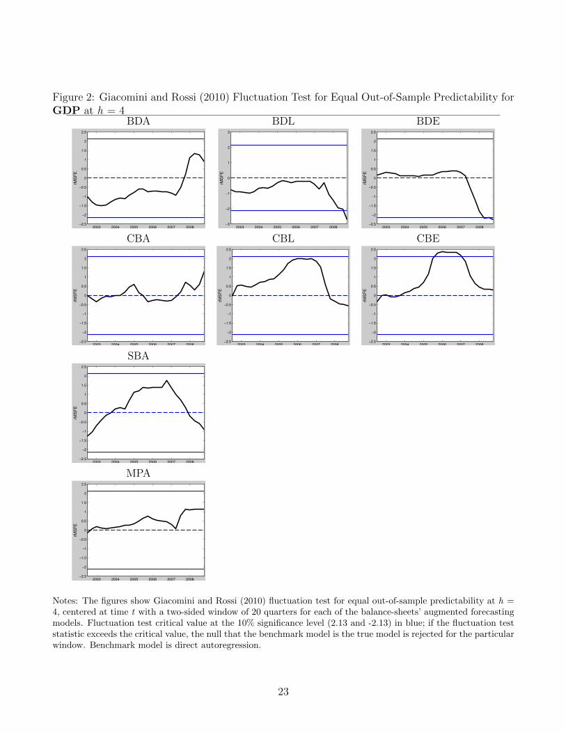
Figure 2: Giacomini and Rossi (2010) Fluctuation Test for Equal Out-of-Sample Predictability forGDP at h = 4

BDA BDL BDE

2003 2004 2005 2006 2007 2008−2.5

−2

−1.5

−1

−0.5

0

0.5

1

1.5

2

2.5

rMS

FE

2003 2004 2005 2006 2007 2008−3

−2

−1

0

1

2

3

rMS

FE

2003 2004 2005 2006 2007 2008−2.5

−2

−1.5

−1

−0.5

0

0.5

1

1.5

2

2.5

rMS

FE

CBA CBL CBE

2003 2004 2005 2006 2007 2008−2.5

−2

−1.5

−1

−0.5

0

0.5

1

1.5

2

2.5

rMS

FE

2003 2004 2005 2006 2007 2008−2.5

−2

−1.5

−1

−0.5

0

0.5

1

1.5

2

2.5

rMS

FE

2003 2004 2005 2006 2007 2008−2.5

−2

−1.5

−1

−0.5

0

0.5

1

1.5

2

2.5

rMS

FE

SBA

2003 2004 2005 2006 2007 2008−2.5

−2

−1.5

−1

−0.5

0

0.5

1

1.5

2

2.5

rMS

FE

MPA

2003 2004 2005 2006 2007 2008−2.5

−2

−1.5

−1

−0.5

0

0.5

1

1.5

2

2.5

rMS

FE

Notes: The figures show Giacomini and Rossi (2010) fluctuation test for equal out-of-sample predictability at h =4, centered at time t with a two-sided window of 20 quarters for each of the balance-sheets’ augmented forecastingmodels. Fluctuation test critical value at the 10% significance level (2.13 and -2.13) in blue; if the fluctuation teststatistic exceeds the critical value, the null that the benchmark model is the true model is rejected for the particularwindow. Benchmark model is direct autoregression.

23

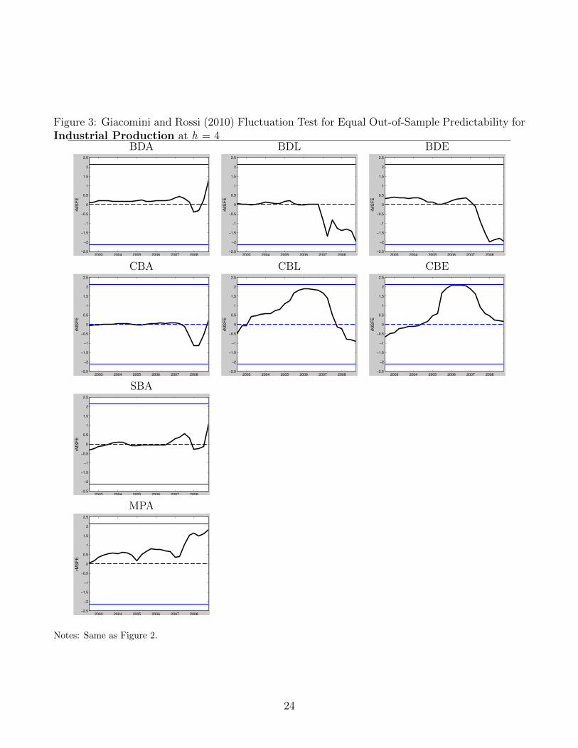
Figure 3: Giacomini and Rossi (2010) Fluctuation Test for Equal Out-of-Sample Predictability forIndustrial Production at h = 4

BDA BDL BDE

2003 2004 2005 2006 2007 2008−2.5

−2

−1.5

−1

−0.5

0

0.5

1

1.5

2

2.5

rMS

FE

2003 2004 2005 2006 2007 2008−2.5

−2

−1.5

−1

−0.5

0

0.5

1

1.5

2

2.5

rMS

FE

2003 2004 2005 2006 2007 2008−2.5

−2

−1.5

−1

−0.5

0

0.5

1

1.5

2

2.5

rMS

FE

CBA CBL CBE

2003 2004 2005 2006 2007 2008−2.5

−2

−1.5

−1

−0.5

0

0.5

1

1.5

2

2.5

rMS

FE

2003 2004 2005 2006 2007 2008−2.5

−2

−1.5

−1

−0.5

0

0.5

1

1.5

2

2.5

rMS

FE

2003 2004 2005 2006 2007 2008−2.5

−2

−1.5

−1

−0.5

0

0.5

1

1.5

2

2.5

rMS

FE

SBA

2003 2004 2005 2006 2007 2008−2.5

−2

−1.5

−1

−0.5

0

0.5

1

1.5

2

2.5

rMS

FE

MPA

2003 2004 2005 2006 2007 2008−2.5

−2

−1.5

−1

−0.5

0

0.5

1

1.5

2

2.5

rMS

FE

Notes: Same as Figure 2.

24

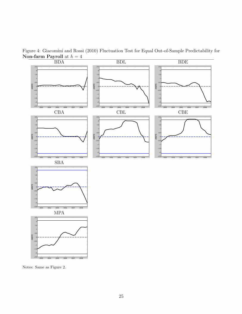
Figure 4: Giacomini and Rossi (2010) Fluctuation Test for Equal Out-of-Sample Predictability forNon-farm Payroll at h = 4

BDA BDL BDE

2003 2004 2005 2006 2007 2008−2.5

−2

−1.5

−1

−0.5

0

0.5

1

1.5

2

2.5

rMS

FE

2003 2004 2005 2006 2007 2008−2.5

−2

−1.5

−1

−0.5

0

0.5

1

1.5

2

2.5

rMS

FE

2003 2004 2005 2006 2007 2008−2.5

−2

−1.5

−1

−0.5

0

0.5

1

1.5

2

2.5

rMS

FE

CBA CBL CBE

2003 2004 2005 2006 2007 2008−2.5

−2

−1.5

−1

−0.5

0

0.5

1

1.5

2

2.5

rMS

FE

2003 2004 2005 2006 2007 2008−2.5

−2

−1.5

−1

−0.5

0

0.5

1

1.5

2

2.5

rMS

FE

2003 2004 2005 2006 2007 2008−2.5

−2

−1.5

−1

−0.5

0

0.5

1

1.5

2

2.5

rMS

FE

SBA

2003 2004 2005 2006 2007 2008−2.5

−2

−1.5

−1

−0.5

0

0.5

1

1.5

2

2.5

rMS

FE

MPA

2003 2004 2005 2006 2007 2008−2.5

−2

−1.5

−1

−0.5

0

0.5

1

1.5

2

2.5

rMS

FE

Notes: Same as Figure 2.

25

Figure 5: Giacomini and Rossi (2010) Fluctuation Test for Equal Out-of-Sample Predictability forInvestment at h = 4

BDA BDL BDE

2003 2004 2005 2006 2007 2008−2.5

−2

−1.5

−1

−0.5

0

0.5

1

1.5

2

2.5

rMS

FE

2003 2004 2005 2006 2007 2008−2.5

−2

−1.5

−1

−0.5

0

0.5

1

1.5

2

2.5

rMS

FE

2003 2004 2005 2006 2007 2008−2.5

−2

−1.5

−1

−0.5

0

0.5

1

1.5

2

2.5

rMS

FE

CBA CBL CBE

2003 2004 2005 2006 2007 2008−2.5

−2

−1.5

−1

−0.5

0

0.5

1

1.5

2

2.5

rMS

FE

2003 2004 2005 2006 2007 2008−2.5

−2

−1.5

−1

−0.5

0

0.5

1

1.5

2

2.5

rMS

FE

2003 2004 2005 2006 2007 2008−3

−2

−1

0

1

2

3

rMS

FE

SBA

2003 2004 2005 2006 2007 2008−2.5

−2

−1.5

−1

−0.5

0

0.5

1

1.5

2

2.5

rMS

FE

MPA

2003 2004 2005 2006 2007 2008−2.5

−2

−1.5

−1

−0.5

0

0.5

1

1.5

2

2.5

rMS

FE

Notes: Same as Figure 2.

26

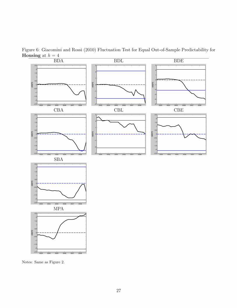
Figure 6: Giacomini and Rossi (2010) Fluctuation Test for Equal Out-of-Sample Predictability forHousing at h = 4

BDA BDL BDE

2003 2004 2005 2006 2007 2008−2.5

−2

−1.5

−1

−0.5

0

0.5

1

1.5

2

2.5

rMS

FE

2003 2004 2005 2006 2007 2008−3

−2

−1

0

1

2

3

rMS

FE

2003 2004 2005 2006 2007 2008−5

−4

−3

−2

−1

0

1

2

3

rMS

FE

CBA CBL CBE

2003 2004 2005 2006 2007 2008−2.5

−2

−1.5

−1

−0.5

0

0.5

1

1.5

2

2.5

rMS

FE

2003 2004 2005 2006 2007 2008−3

−2

−1

0

1

2

3

rMS

FE

2003 2004 2005 2006 2007 2008−2.5

−2

−1.5

−1

−0.5

0

0.5

1

1.5

2

2.5

rMS

FE

SBA

2003 2004 2005 2006 2007 2008−2.5

−2

−1.5

−1

−0.5

0

0.5

1

1.5

2

2.5

rMS

FE

MPA

2003 2004 2005 2006 2007 2008−2.5

−2

−1.5

−1

−0.5

0

0.5

1

1.5

2

2.5

rMS

FE

Notes: Same as Figure 2.

27

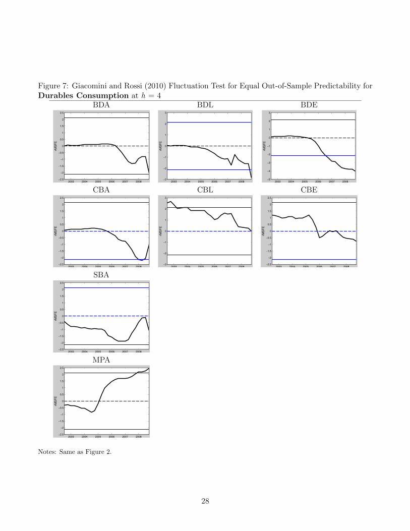
Figure 7: Giacomini and Rossi (2010) Fluctuation Test for Equal Out-of-Sample Predictability forDurables Consumption at h = 4

BDA BDL BDE

2003 2004 2005 2006 2007 2008−2.5

−2

−1.5

−1

−0.5

0

0.5

1

1.5

2

2.5

rMS

FE

2003 2004 2005 2006 2007 2008−3

−2

−1

0

1

2

3

rMS

FE

2003 2004 2005 2006 2007 2008−5

−4

−3

−2

−1

0

1

2

3

rMS

FE

CBA CBL CBE

2003 2004 2005 2006 2007 2008−2.5

−2

−1.5

−1

−0.5

0

0.5

1

1.5

2

2.5

rMS

FE

2003 2004 2005 2006 2007 2008−3

−2

−1

0

1

2

3

rMS

FE

2003 2004 2005 2006 2007 2008−2.5

−2

−1.5

−1

−0.5

0

0.5

1

1.5

2

2.5

rMS

FE

SBA

2003 2004 2005 2006 2007 2008−2.5

−2

−1.5

−1

−0.5

0

0.5

1

1.5

2

2.5

rMS

FE

MPA

2003 2004 2005 2006 2007 2008−2.5

−2

−1.5

−1

−0.5

0

0.5

1

1.5

2

2.5

rMS

FE

Notes: Same as Figure 2.

28