balance sheet effects on monetary and financial spillovers ...mchinn/aci-spillover07_22_2016.pdf ·...
TRANSCRIPT

Preliminary version: July 22, 2016
Balance Sheet Effects on Monetary and Financial Spillovers:
The East Asian Crisis Plus 20
Joshua Aizenman*, Menzie D. Chinn†, Hiro Ito‡
USC and NBER; UW-Madison and NBER; Portland State University
Abstract
We study how the financial conditions in the Center Economies [the U.S., Japan, and the Euro area]
impact other countries, over the period 1986 through 2015. Our methodology relies upon a two-step
approach. We focus on five possible linkages between the center economies (CEs) and the non-Center
economics, or peripheral economies (PHs), and investigate the strength of these linkages. For each of the
five linkages, we first regress a financial variable of the PHs on financial variables of the CEs while
controlling for global factors. Next, we examine the determinants of sensitivity to the CEs as a function of
country-specific macroeconomic conditions and policies, including the exchange rate regime, currency
weights, monetary, trade and financial linkages with the CEs, the levels of institutional development, and
international reserves. Extending our previous work (Aizenman et al. (2015)), we devote special attention
to the impact of currency weights in the implicit currency basket, balance sheet exposure, and currency
composition of external debt. Our results support the view that there is no way for countries to fully
insulate themselves from shocks originating from the CEs. We find that for both policy interest rates and
the real exchange rate (REER), the link with the CEs has been pervasive for developing and emerging
market economies in the last two decades, although the movements of policy interest rates are found to be
more sensitive to global financial shocks around the time of the emerging markets’ crises in the late 1990s
and early 2000s, and since 2008. When we estimate the determinants of the extent of connectivity, we
find evidence that the weights of major currencies, external debt, and currency compositions of debt are
significant factors. More specifically, having a higher weight on the dollar (or the euro) makes the
response of a financial variable such as the REER and exchange market pressure in the PHs more
sensitive to a change in key variables in the U.S. (or the euro area) such as policy interest rates and the
REER. While having more exposure to external debt would have similar impacts on the financial linkages
between the CEs and the PHs, the currency composition of international debt securities matter.
Economies more reliant on dollar-denominated debt issuance tend to be more vulnerable to shocks
emanating from the U.S.
* Aizenman: Dockson Chair in Economics and International Relations, University of Southern California,
University Park, Los Angeles, CA 90089-0043. Phone: +1-213-740-4066. Email: [email protected]. † Chinn: Robert M. La Follette School of Public Affairs; and Department of Economics, University of
Wisconsin, 1180 Observatory Drive, Madison, WI 53706. Phone: +1-608-262-7397. Email:
[email protected] . ‡ Ito (corresponding author): Department of Economics, Portland State University, 1721 SW Broadway,
Portland, OR 97201. Tel/Fax: +1-503-725-3930/3945. Email: [email protected] .
Acknowledgements: The financial support of faculty research funds of University of Southern California, the
University of Wisconsin, Madison, and Portland State University is gratefully acknowledged. All remaining
errors are ours.
2
1. Introduction
On the eve of the 20th year anniversary of the East Asian crisis, we investigate the impact
of balance sheet exposures, economic structure and trilemma choices on the exposure of
countries to shocks emanating from the center. Events over recent decades have vividly
illustrated that balance sheet exposure impact monetary and fiscal spaces, capital mobility, and
exchange market pressure. The evolution of global dynamics during the post-Global Financial
Crisis period led Rey (2013) to propound the hypothesis that exchange rate regimes no longer
insulated countries from global financial cycles – in other words, the demise of the Mundellian
Trilemma. In order to gain further insights regarding these developments, we examine how the
financial conditions of -- and shocks propagated from -- the Center Economies [dubbed CEs,
namely the U.S., Japan, and the Euro area], impact the non CEs economics.
Our empirical method relies upon a two-step approach. We first investigate the extent of
sensitivity of policy interest rate, the real effective exchange rate and several other macro
variables to those of the center economies while controlling for global factors. The estimation is
done for the sample period is 1986 through 2015, using monthly data and in a rolling fashion.
Next, we examine the association of these sensitivity coefficients with country’s trilemma
choices, the real and financial linkages with the center economy, the levels of institutional
development, balance sheet exposure, and the like. Using the methodology of Frankel and Wei
(1996), we estimate the currency weights of the non-ECs economies, and we study the impact of
these weights on the transmission of shocks from the ECs to non-ECs countries (or peripheral
economies, “PHs”).
We find that for both policy interest rates and the real exchange rate [REER], the link
with the CEs has been a dominant factor for developing and emerging market economies
[EMGs] in the last two decades. Furthermore, the developing and EMGs policy interest rates are
more sensitive to global financial shocks around the time of EMGs’ crises in the period
surrounding the turn of the century, and again since the Global Financial Crisis [GFC] of 2008.
In contrast with Rey’s conclusions, we find that the type of exchange rate regime and country’s
currency weights do matter: developing countries or emerging market economies with more
stable exchange rate and more open financial markets are more affected by changes in the policy
interest rates in the CEs. Notably, holding higher levels of foreign reserves tend to help PHs to
shield the impact of changes in the CEs’ policy interest rates, i.e., to retain its monetary
3
autonomy. Exchange rate stability, financial openness, and IR holding are jointly significant for
the group of developing or emerging market countries. As for the external links, financial
linkage through foreign direct investment [FDI] is the most important variable in determining
how shocks of CEs’ monetary policies affect those of other PHs for both developing and EMGs.
A country that receives more FDI from the CE’s tends to be more sensitive to changes in the
monetary policies of the CEs.
Our results show the positive impact of greater exchange rate stability on the REER
connectivity for all the subsample country groups. Greater financial openness also contributes to
greater sensitivity for developing countries, though not significantly as for the EMGs group.
Emerging market countries with larger government debt tend to be less sensitive to the REER of
the center economies. These results may reflect the fact that such countries, which likely face
higher inflationary expectations, often confront challenges in maintaining real exchange rate
stability against the currencies of the major economies despite their general desire to pursue
greater nominal exchange rate stability.
Countries with greater bilateral trade links with the center economies tend to be more
sensitive to the REER movements of the center economies, while countries with more developed
financial markets tend to be less sensitive to the REER movements of the CEs. These results are
consistent with the observation that greater financial development allows a country to have more
flexible exchange rate movements. In other words, such countries can afford to detach their
currency values’ movements from those of the center economies.
Finally, and distinct from our earlier results, we find evidence that the weights of major
currencies, the extent of external debt, and the currency composition of debt are significant
factors. Having a higher weight of the dollar (or the euro) enhances the responsiveness of a
financial variable such as PH REER and EMP to a change in key variables in the U.S. (or the
euro area). While having more exposure to external debt has similar effects on the financial
linkages between the CEs and the PHs, the currency composition of international debt securities
has a differential impact. Those economies more reliant on the dollar for debt issuance tend to be
more vulnerable to shocks occurring in the U.S.
Overall, we find that open macro policy arrangements have not only direct but also
indirect impacts on the linkage between the CEs’ policy interest rates, REER, on developing

4
countries’ EMP. Hence, we can conclude that trilemma policy arrangements do affect the
sensitivity of developing countries to policy changes in the center economies.
2 The Framework of the Main Empirical Analysis
Methodologically, we extend the same approach as followed in Aizenman et al. (2015),
with special focus on different determinants of linkage strength between the CEs and the PHs. To
recap, our analytical process is similar to the two-step estimations employed by Forbes and
Chinn (2004). As the first step, we focus on the five possible linkages between the PHs and the
CEs and investigate the degree of the sensitivity through those linkages. For each of the five
paths of linkages, we regress a financial variable of the PHs on another (or the same) variable of
the CEs while controlling for global factors. In the second step, we treat the estimated degree of
sensitivity as the dependent variable, and examine their determinants among a number of
country-specific variables, including the roles of countries’ macroeconomic conditions or
policies, real or financial linkage with the center economy, or the level of institutional
development of the countries. In this study, our discussion centers on the effect of variables
pertaining to balance sheets of the sample countries such as external debt, the weights of major
currencies in the currency basket, and the share of currencies for debt denomination.
2.1 The Five Path of Linkages – The Channels through which PHs are Susceptible to
Changes in CEs’ Financial Conditions
Before we investigate the linkages between the CEs and the PHs, we must identify what
kind of path of linkages we focus on. In that regard, Figure 1 is helpful. It illustrates how the
variables of our focus tend to be more affected by spillovers of shocks around the globe. More
specifically, the five paths of linkages between the CEs and the PHs are as follows.
Link 1 – Short-term, policy interest rate in the CEs Short-term, policy interest rate in
the PHs: If country i has its monetary policy more susceptible to the monetary policy of one (or
more) of the CEs, the correlation of the policy interest rates between the CEs and PHs is should
be significantly positive, implying a closer linkage between the CEs and PHs. However, a
significantly negative correlation could also mean a closer linkage. If a rise in a CE’s policy rate
could draw capital from the PHs, that could reduce money demand among PHs and therefore
5
lower the policy rates among them while the CEs experience a rise in both money demand and
the policy rate, thus making the correlation negative.4
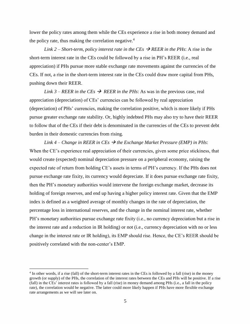
Link 2 – Short-term, policy interest rate in the CEs REER in the PHs: A rise in the
short-term interest rate in the CEs could be followed by a rise in PH’s REER (i.e., real
appreciation) if PHs pursue more stable exchange rate movements against the currencies of the
CEs. If not, a rise in the short-term interest rate in the CEs could draw more capital from PHs,
pushing down their REER.
Link 3 – REER in the CEs REER in the PHs: As was in the previous case, real
appreciation (depreciation) of CEs’ currencies can be followed by real appreciation
(depreciation) of PHs’ currencies, making the correlation positive, which is more likely if PHs
pursue greater exchange rate stability. Or, highly indebted PHs may also try to have their REER
to follow that of the CEs if their debt is denominated in the currencies of the CEs to prevent debt
burden in their domestic currencies from rising.
Link 4 – Change in REER in CEs the Exchange Market Pressure (EMP) in PHs:
When the CE’s experience real appreciation of their currencies, given some price stickiness, that
would create (expected) nominal depreciation pressure on a peripheral economy, raising the
expected rate of return from holding CE’s assets in terms of PH’s currency. If the PHs does not
pursue exchange rate fixity, its currency would depreciate. If it does pursue exchange rate fixity,
then the PH’s monetary authorities would intervene the foreign exchange market, decrease its
holding of foreign reserves, and end up having a higher policy interest rate. Given that the EMP
index is defined as a weighted average of monthly changes in the rate of depreciation, the
percentage loss in international reserves, and the change in the nominal interest rate, whether
PH’s monetary authorities pursue exchange rate fixity (i.e., no currency depreciation but a rise in
the interest rate and a reduction in IR holding) or not (i.e., currency depreciation with no or less
change in the interest rate or IR holding), its EMP should rise. Hence, the CE’s REER should be
positively correlated with the non-center’s EMP.
4 In other words, if a rise (fall) of the short-term interest rates in the CEs is followed by a fall (rise) in the money
growth (or supply) of the PHs, the correlation of the interest rates between the CEs and PHs will be positive. If a rise
(fall) in the CEs’ interest rates is followed by a fall (rise) in money demand among PHs (i.e., a fall in the policy
rate), the correlation would be negative. The latter could more likely happen if PHs have more flexible exchange
rate arrangements as we will see later on.
6
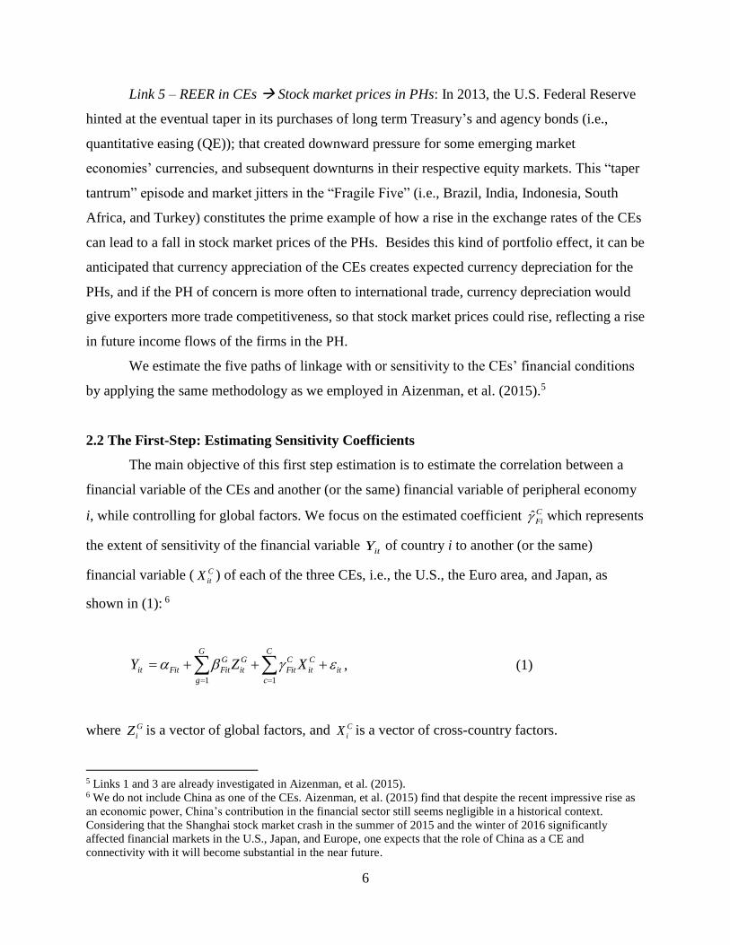
Link 5 – REER in CEs Stock market prices in PHs: In 2013, the U.S. Federal Reserve
hinted at the eventual taper in its purchases of long term Treasury’s and agency bonds (i.e.,
quantitative easing (QE)); that created downward pressure for some emerging market
economies’ currencies, and subsequent downturns in their respective equity markets. This “taper
tantrum” episode and market jitters in the “Fragile Five” (i.e., Brazil, India, Indonesia, South
Africa, and Turkey) constitutes the prime example of how a rise in the exchange rates of the CEs
can lead to a fall in stock market prices of the PHs. Besides this kind of portfolio effect, it can be
anticipated that currency appreciation of the CEs creates expected currency depreciation for the
PHs, and if the PH of concern is more often to international trade, currency depreciation would
give exporters more trade competitiveness, so that stock market prices could rise, reflecting a rise
in future income flows of the firms in the PH.
We estimate the five paths of linkage with or sensitivity to the CEs’ financial conditions
by applying the same methodology as we employed in Aizenman, et al. (2015).5
2.2 The First-Step: Estimating Sensitivity Coefficients
The main objective of this first step estimation is to estimate the correlation between a
financial variable of the CEs and another (or the same) financial variable of peripheral economy
i, while controlling for global factors. We focus on the estimated coefficient C
Fi which represents
the extent of sensitivity of the financial variable itY of country i to another (or the same)
financial variable ( C
itX ) of each of the three CEs, i.e., the U.S., the Euro area, and Japan, as
shown in (1): 6
it
C
c
C
it
C
Fit
G
g
G
it
G
FitFitit XZY 11
, (1)
where G
iZ is a vector of global factors, and C
iX is a vector of cross-country factors.
5 Links 1 and 3 are already investigated in Aizenman, et al. (2015). 6 We do not include China as one of the CEs. Aizenman, et al. (2015) find that despite the recent impressive rise as
an economic power, China’s contribution in the financial sector still seems negligible in a historical context.
Considering that the Shanghai stock market crash in the summer of 2015 and the winter of 2016 significantly
affected financial markets in the U.S., Japan, and Europe, one expects that the role of China as a CE and
connectivity with it will become substantial in the near future.
7
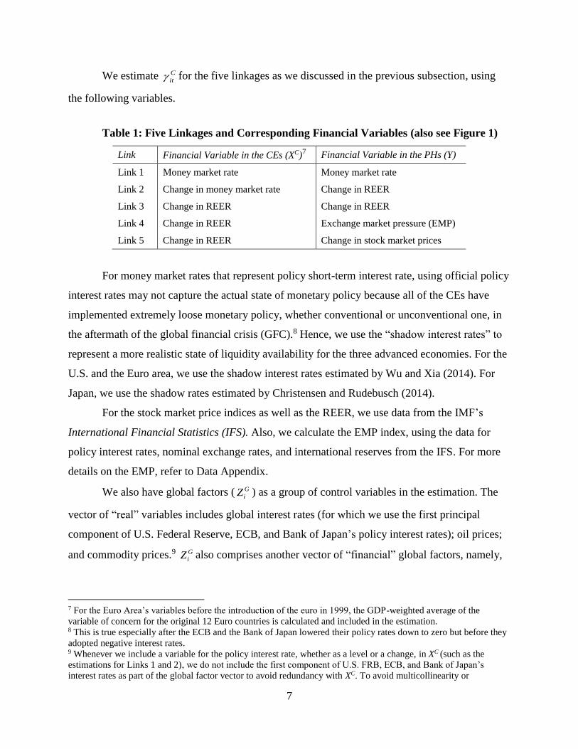
We estimate C
it for the five linkages as we discussed in the previous subsection, using
the following variables.
Table 1: Five Linkages and Corresponding Financial Variables (also see Figure 1)
Link Financial Variable in the CEs (XC)7 Financial Variable in the PHs (Y)
Link 1 Money market rate Money market rate
Link 2 Change in money market rate Change in REER
Link 3 Change in REER Change in REER
Link 4 Change in REER Exchange market pressure (EMP)
Link 5 Change in REER Change in stock market prices
For money market rates that represent policy short-term interest rate, using official policy
interest rates may not capture the actual state of monetary policy because all of the CEs have
implemented extremely loose monetary policy, whether conventional or unconventional one, in
the aftermath of the global financial crisis (GFC).8 Hence, we use the “shadow interest rates” to
represent a more realistic state of liquidity availability for the three advanced economies. For the
U.S. and the Euro area, we use the shadow interest rates estimated by Wu and Xia (2014). For
Japan, we use the shadow rates estimated by Christensen and Rudebusch (2014).
For the stock market price indices as well as the REER, we use data from the IMF’s
International Financial Statistics (IFS). Also, we calculate the EMP index, using the data for
policy interest rates, nominal exchange rates, and international reserves from the IFS. For more
details on the EMP, refer to Data Appendix.
We also have global factors ( G
iZ ) as a group of control variables in the estimation. The
vector of “real” variables includes global interest rates (for which we use the first principal
component of U.S. Federal Reserve, ECB, and Bank of Japan’s policy interest rates); oil prices;
and commodity prices.9 G
iZ also comprises another vector of “financial” global factors, namely,
7 For the Euro Area’s variables before the introduction of the euro in 1999, the GDP-weighted average of the
variable of concern for the original 12 Euro countries is calculated and included in the estimation. 8 This is true especially after the ECB and the Bank of Japan lowered their policy rates down to zero but before they
adopted negative interest rates. 9 Whenever we include a variable for the policy interest rate, whether as a level or a change, in XC (such as the
estimations for Links 1 and 2), we do not include the first component of U.S. FRB, ECB, and Bank of Japan’s
interest rates as part of the global factor vector to avoid redundancy with XC. To avoid multicollinearity or

8
the VIX index from the Chicago Board Options Exchange as a proxy for the extent of investors’
risk aversion as well as the “Ted spread,” which is the difference between the 3-month
Eurodollar Deposit Rate in London (LIBOR) and the 3-month U.S. Treasury Bill yield. The
latter measure gauges the general level of stress in the money market for financial institutions.
We implement the estimation for each of the sample countries for the five links and for
about 100 countries, which include advanced economies (IDC), less developed countries (LDC),
and emerging market countries (EMG) the latter of which is a subset of LDC.10 Inevitably, the
sample size varies depending on data availability. The sample period is 1986 through 2015, using
monthly data, with regressions implemented over non-overlapping three year periods. That
means that we obtain time-varying C
Fit across the panels. For all the estimations, we exclude the
U.S. and Japan. As for the Euro member countries, they are removed from the sample after the
introduction of the euro in January 1999 or they become member countries, whichever comes
first.
2.3 The Second Step: Baseline Model
Once we estimate C
Fit for each of the dependent variables, we regress C
Fit on a number of
country-specific variables. To account for potential outliers on the dependent variable, we apply
the robust regression estimation technique to the following estimation model.
FitFitFitFitFitFit
C
Fit uCRISISINSTLINKMCOMP 543210ˆ (2)
There are four groups of explanatory variables. The first group of explanatory variables is
a set of open macroeconomic policy choices ( iOMP ), for which we include the indexes for
exchange rate stability (ERS) and financial openness (KAOPEN) from the trilemma indexes by
Aizenman, et al. (2013). As another variable potentially closely related to the trilemma
redundancy, we also use the first principal component of oil and commodity prices as a control variable for input or
commodity prices. 10 The emerging market countries (EMG) are defined as the countries classified as either emerging or frontier during
the period of 1980-1997 by the International Financial Corporation plus Hong Kong and Singapore.
9
framework, we include the variable for IR holding (excluding gold) as a share of GDP because
we believe the level of IR holding may affect the extent of cross-country financial linkages.12
The group iMC includes macroeconomic conditions such as inflation volatility, current
account balance, and public finance conditions. As the measure of public finance conditions, we
include gross national debt expressed as a share of GDP.
In addition, we include variables that reflect the extent of linkages with the center
countries (LINK). One linkage variable is meant to capture real, trade linkage, which we measure
as: ip
C
ipip GDPIMPLINKTR _ where C
iIMP is total imports into center economy C from
country i, that is normalized by country i’s GDP. Another linkage variable is financial linkage,
FIN_LINKip. We measure it with the ratio of the total FDI stock and bank lending from country
C in country i both as shares of country i’s GDP.
Another variable that also reflects the linkage with the major economies is the variable
for the extent of trade competition (Trade_Comp). Trade_Comp measures the importance to
country i of export competition in the third markets between country i and major country C.
Shocks to country C, and especially shocks to country C that affects country c’s exchange rate,
could affect the relative price of country C’s exports and therefore affect country i through trade
competition in third markets. See Appendix for the variable construction. A higher value of this
measure indicates country i and major economic C exports products in similar sectors so that
their exported products tend to be competitive to each other.
The fourth group is composed of the variables that characterize the nature of institutional
development (INST), namely, variables for financial development and legal development. For the
measure of the level of financial development, we use the first principal component of financial
development using the data on private credit creation, stock market capitalization, stock market
total value, and private bond market capitalization all as shares of GDP. Likewise, we measure
the level of legal development using the first principal component of law and order (LAO),
bureaucratic quality (BQ), and anti-corruption measures (CORRUPT). Higher values of these
variables indicate better conditions.
To control for economic or financial disruptions, we include a vector of currency and
banking crises (CRISIS). For currency crisis, we use the exchange market pressure (EMP) index
12 Aizenman, et al. (2010, 2011) show the macroeconomic impact of trilemma policy configurations depends upon
the level of IR holding.
10
using the exchange rate against the currency of the base country. The banking crisis dummy is
based on the papers by Laeven and Valencia (2008, 2010, 2012).
The variables in MC and INST are included in the estimations as deviations from the
U.S., Japanese, and Euro Area’s counterparts. The variables in vectors OMP, MC, and INST are
sampled from the first year of each three year panels to minimize the effect of potential
endogeneity. Also, in order to capture global common shocks, we also include time fixed effects.
3 Empirical Results for the Baseline Estimation
3.1 First-Step Estimations – Connectivity with the CEs
As the first step, we estimate the extent of correlation for each of the five financial
linkages while controlling for two kinds of global factors: “real global” and “financial global,”
using the three-year, non-overlapping panels in the 1986-2015 period.
To gain a birds-eye view of the empirical results and the general trend of the groups of
factors that influence the financial links, we focus on the joint significance of the variables
included in the real global and financial global groups, and vector XC the latter of which includes
the financial variables of the CEs for each of the five potential financial links (Table 1 and
Figure 1).
Figure 2 illustrates the proportion of countries for which the joint significance tests are
found to be statistically significant (with the p-value less than 5%) for the real global and
financial global groups, and vector XC for the five financial links. While we present the
proportion for the groups of advanced economies (IDC) and less developed economies (LDC)
after 1992, our discussions focuses on the results of developing countries.13
The graphical depictions in Figure 2 lead to the following conclusions. First, the
influence of the CEs is the greatest for the policy interest rates and the real effective exchange
rates. That is, the policy interest rates and the REER of the CEs affect most joint-significantly
those of the PHs, respectively. This is consistent with the findings reported in Aizenman, et al.
(2015).
Second, the REER of the CEs significantly affects the stock market price changes of the
PHs during and after the Global Financial Crisis [GFC] of 2008, though the impact dwindles
13 We also conduct the same exercise for the subgroup of EMGs. The figures for the EMG group are usually
qualitatively similar to those of the LDC group. Hence, we omit discussing them here.
11
toward the end of the sample period. This and previous findings are consistent with the reactions
expressed by emerging market policy makers – especially those in “Fragile Five” – to the taper
in Fed quantitative easing and the Federal Fund rate increase in December 2015.
Third, the policy interest rates of the CEs do not affect the REER of many PHs. Even
during the GFC and its immediate aftermath, the proportion of the countries for which the policy
interest rates of the CEs are jointly significant is about 20%. A similar observation can be made
for the REER-EMP link.
Fourth, as far as the policy interest rate link between the CEs and the PHs (Link 1) is
concerned, the proportion of joint significance is also relatively high for the group of “financial
global” variables during the GFC and the last three year panel for developing countries and since
the GFC for developed countries and emerging market countries, suggesting global financial
factors have been playing an important role in affecting the policy interest of countries regardless
of income levels. This result is consistent with the Rey’s (2013) thesis of “global financial
cycles.” Not surprisingly, economies are more exposed to global financial shocks during periods
of financial turbulence while also following CEs’ monetary policies.
Figure 3 disaggregates the effect of the CEs. The bars illustrate the proportion of the
countries with significant 𝛾’s for the three CEs: the United States, the euro area, and Japan. We
see the U.S. financial variables exerting the most significant effects on the financial variables of
the PHs for the policy interest rate link and the REER link in most of the time period, and for the
REER-stock market price link during the GFC years. For the policy interest rate and the REER
links, we see the euro area affecting the financial variables of the PHs as well.
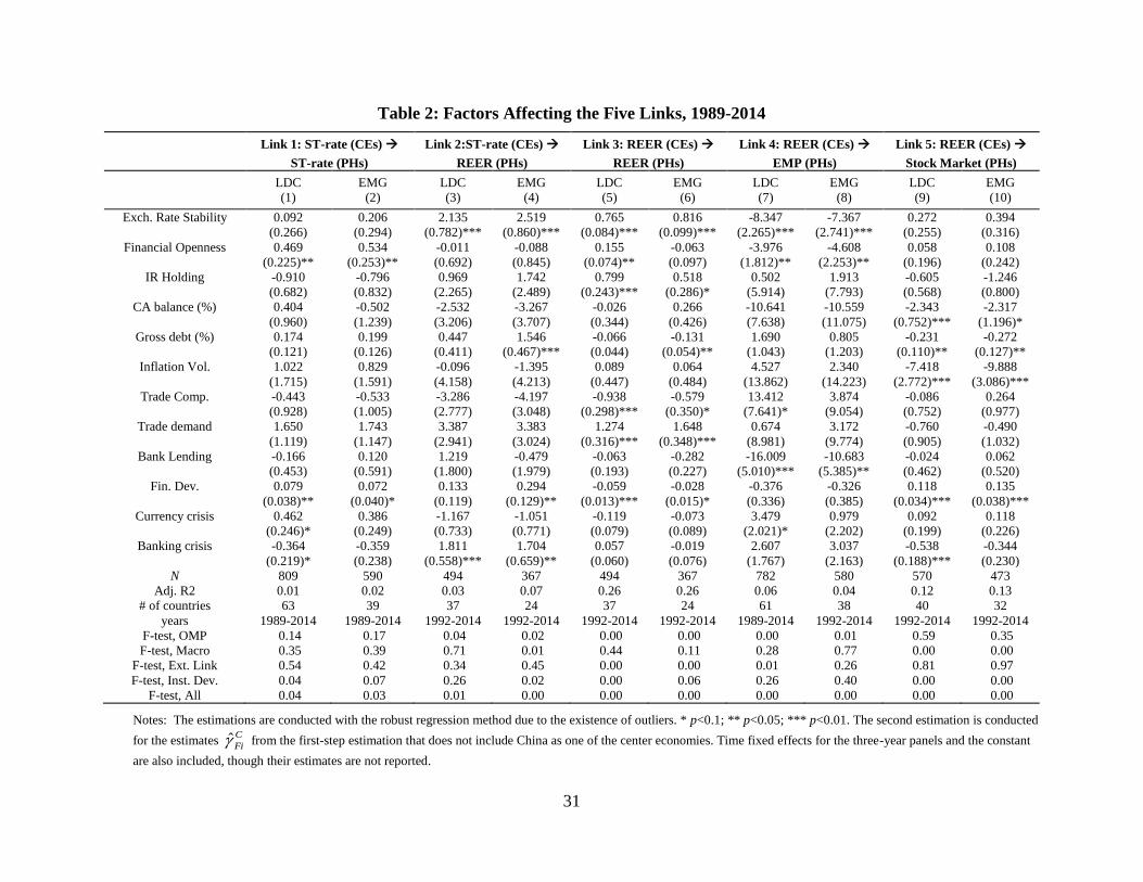
3.2 Results of the Second-Step Estimation
Now, we investigate the determinants of the extent of linkages, C
Fit , using the estimation
model based on equation (2). Table 2 reports the estimation results for the five linkages for the
LDC and EMG samples. The bottom rows of the tables also report the joint significance tests for
each vector of explanatory variables.
We begin by discussing the results for the open macro policy arrangements, namely,
exchange rate stability, financial openness, and IR holding. While PHs with more open financial
markets tend to follow the monetary policy of the CEs, the extent of exchange rate stability they
pursue does not matter (columns 1 and 2). Aizenman, et al. (2015) found a significantly positive
12
estimate for the exchange rate variable, but our estimates are also positive but not statistically
significant.14
The more stable a PH country’s exchange rate movements are, the more sensitive its
REER to the CEs’ policy interest rates or REER (columns 3-6). These results make sense; PHs
preferring more exchange rate stability follow the CEs’ monetary policy or real appreciation of
the CEs’ currencies, which is what we have observed among emerging market economies in
2013-15.
Interestingly, higher levels of IR holding would make it easier for both developing and
emerging market countries to follow the currency real appreciation of the CEs, though there is a
possibility this correlation is capturing reverse causality. Also, not surprisingly, PHs with more
open financial markets tend to guide their REER to follow that of the CEs, though such an
observation cannot be made for the EMG group (columns 5 and 6).
When the CEs experience real appreciation, the more exchange rate stability a PH
pursues, the less pressure it faces on its EMP (columns 7 and 8). At the same time, if the PH has
more open financial markets, it would face less pressure on its EMP when the CEs’ currencies
are appreciating in real terms. The interpretation of this result is difficult; it could be that more
open financial markets are associated with more developed financial markets, that are more
robust to shocks emanating from abroad. Alternatively, countries that are subject to shocks tend
to implement capital controls.
Open macro policies do not seem to matter for the link between the CEs’ REER and the
PHs’ stock market price movements (columns 9 and 10). The F-test for the joint significance for
the open macro variables is far from significant. Instead, the groups of macroeconomic
conditions and institutional characteristics are found to be jointly significant. Interestingly, PHs
with higher debt levels or higher levels of inflation volatility tend to have their stock market
prices falling when the CEs experience currency real appreciation. We infer that weak
macroeconomic conditions lead to capital flight once the CEs experience real appreciation,
which in turn leads equity market declines. The negative estimate on the current account variable
indicates that while PHs running current account deficit tend to experience real depreciation
14 We do not include the growth rate of industrial production in the first-step estimation to maximize the sample size
of the gammas. This, along with the extended sample period, may explain the different estimation results for the
exchange rate stability index.
13
when the CEs’ currencies appreciate in real terms, weaker currencies of PHs could allow their
firms to experience a rise in their income flows, pushing up the stock market prices in those
economies.
4. Impacts of Currency Weights and External Debt
In addition to the baseline model, we investigate the impact of other factors, especially
those which are related to the balance sheets of the countries. The first factor we investigate is
the extent of belonging to the dollar or euro zone. Clearly, the United States was the epicenter of
the GFC. That means that countries that are dollar-oriented or dollar centric in their trade of
goods and services as well as financial assets must have been more exposed to shocks arising
from the U.S. We can make a similar argument about the extent of belonging to the euro zone
especially since the euro area experienced the debt crisis in the 2010s.
The other factor, closely linked with the previous factor, is how exposed countries are in
terms of being indebted externally. Highly indebted countries can be more susceptible to external
shocks, especially if the debt is denominated in foreign currencies. We also investigate the
interactive effects of external debt exposure and the extent of reliance on the major currencies for
debt denomination.
This is a timely question. For the last two decades, the extent of “original sin” – the
inability of developing countries to issue debt in their domestic currencies in international
markets – has been perceived to be declining.15 That stands in contrast to the situation during
emerging market crises of the 1980s through early 2000’s, when all external debt was essentially
foreign currency denominated debt. In such cases, cross border asset-liability currency
mismatches combined with large cross-border holdings meant that currency depreciations could
easily cause liquidity crises.
4.1 Impacts of Currency Weights and Trade with Currency Zones
4.1.1 Model Framework
15 See Hausmann and Panizza (2011), who argue that the decline in the extent of original sin has been only anecdotal
by showing that the decline in original sin has been modest if any. Ito and Rodriguez (2015) also show that the
extent of reliance on foreign currency denomination for issuing international debt has not changed much for the last
two decades.
14
We now investigate the impact of the extent of belong to a major currency zone. When
PHs’ monetary policy makers make decisions, they almost inevitably incorporate the monetary
policy of the issuer of a major currency which they reference to, or they refer to an implicit
currency basket composed of several major currencies. Hence, once a shock arises in a CE,
reactions by the PHs could be affected by the composition of the major currencies in the implicit
currency basket. That is, the degree of sensitivity among the PHs to the policies and economic
conditions of the CEs can depend upon the weights of the currencies in the basket. In the analysis
below, when, say, the dollar has the highest weight in the basket, we regard the economy of
concern as dollar-oriented or belonging to the dollar zone. The currency weights can be
independent of the degree of exchange rate stability a country pursues.
Using the widely-used method developed by Haldane and Hall (1991) and popularized by
Frankel and Wei (1996), we estimate the weights of the dollar, the euro (or the German deutsche
mark and the French franc before the introduction of the euro in 1999), the yen, and the British
sterling with a rolling window of 36 months.16
With the estimated weights, we can test whether and to what extent the weights of
currencies in the basket affect the extent of connectivity between the CEs and the PHs (i.e., 𝛾’s )
using the following model:
(3) ,
ˆ
,,
7
,
6
543210
Fit
EuroUS
Fit
EuroUS
Fit
EuroUS
Fit
FitFitFitFitFit
C
Fit
uCZWDCZW
CRISISINSTLINKMCOMP
where C refers to the CEs: the U.S., the Euro area, and Japan and F to the five financial linkages.
CZWUS, Euro is the estimated weights for the dollar and the euro. 𝐷Γ represents the dummies for
𝛾𝑈𝑆and 𝛾𝐸𝑢𝑟𝑜.17
16 The basic assumption of this exercise is that monetary authorities use an implicit basket of currencies as the
portfolio of official foreign exchange reserves, but that the extent of response to the change in the value of the entire
basket should vary over time and across countries. If the authorities want to maintain a certain level of exchange rate
stability, whether against a single currency or a basket of several currencies, they should allow the currency value to
adjust only in accordance with the change in the entire value of the basket of major currencies. The examples of the
application of this method can be found in Frankel and Wei (1996) among many others. 17 Keep in mind that we have 𝛾𝑈𝑆, 𝛾𝐸𝑢𝑟𝑜, and 𝛾𝐽𝑃for country i in year t as the dependent variable.
15
We focus on 𝜃7, which includes the interaction term between the dummy for 𝛾𝑈𝑆and the
currency zone weight for the dollar (CZWUS) and the one between the dummy for 𝛾𝐸𝑢𝑟𝑜 and the
currency zone weight for the euro (CZWEuro).
If the extent of belonging to a currency zone matters, 𝜃7 must be statistically significant.
Because we have the two dummies for 𝛾𝑈𝑆and 𝛾𝐸𝑢𝑟𝑜, the sensitivity to a shock in Japan is
treated as the baseline. Hence, 𝜃6 represents how the dollar or euro currency weight affects the
degree of sensitivity to a shock originating in Japan.
Hence, for example, if Korea has a high dollar zone weight, the degree of sensitivity to a
financial shock arising from the U.S. (𝛾𝑈𝑆) should be higher if the dollar zone weight (CZWUS) is
higher. Likewise, the impact of the euro weight can be found in 𝜃7. Also, the dollar or euro zone
weight (CZWUS or Euro) should matter less to the shocks occurring in Japan (𝜃6).18
One merit of having estimated currency weights for our sample countries is that, using
the estimated currency weights, we can divide the currency zones’ partners of each non-major
currency economy into five currency zones.19 To do so, every non-G5 economy is divided into
G5-currency zones, based on the estimated G5-currency weights, i.e.,iht , for the economy. For
example, if Thailand has a currency basket, with the USD weight of a%, the DM weight of b%,
the FF weight of c%, the BP weight of d%, and the yen weight of e%, then we assume that a% of
Thailand’s economy belongs to the USD zone, b% to the DM zone, c% to the FF zone, d% to the
UKP zone, and e% to the yen zone. All other non-G5 economies are similarly divided into G5
currency zones. On the other hand, each of the G5 countries is assumed to constitute its own
currency zone. Then, the trade share of a non-G5 economy (say India) with countries belonging
to a major-currency zone can be calculated first by multiplyingiht with bilateral trade with each
partner (say Thailand, while bilateral trade between India and Thailand is defined as the sum of
bilateral exports and imports), and then by summing up all the products over all the bilateral
trade pairs. The ratio of this sum to the economy’s (India’s) total trade is regarded as its trade
share with one of the “major-currency zones.”20
18 That means 𝜽6 should have the opposite sign to 𝜽7 or be insignificant. 19 The choice of the G5 countries is based on the currencies represented by the SDR basket during the sample
period, see https://www.imf.org/external/np/fin/data/rms_sdrv.aspx.
20 For country i, the currency zone share for major currency h is
it
J
j ijtjht
itTRADE
TRADEhSHARE
_
where j is i’s trading
partner ( Jj ) and 1_ H
h ithSHARE .

16
Now, we include the share of trade with respect to the dollar and the euro zones instead
of the dollar and the euro zone weights as follows:
(4) ._ _
ˆ
,,
7
,
6
543210
Fit
EuroUS
Fit
EuroUS
Fit
EuroUS
Fit
FitFitFitFitFit
C
Fit
uCZTHDCZTH
CRISISINSTLINKMCOMP
Like in the previous case, if the shares of trade with countries in the dollar zone or those
in the euro zone matter, 𝜃7 should be statistically significant, and 𝜃6 would capture the impact of
trade with the dollar or euro zone countries on the sensitivity to a financial shock arising from
Japan.21
4.1.2 Estimation Results
Table 3 reports the results for each of the five link regressions. To conserve space,
however, we only report the estimates for the open macro variables and the variables pertaining
to currency weights.
Although the extent of belonging to the dollar zone does not matter for the link between
the CEs’ policy interest rates and the PHs’ REER (Link 2), it does matter for the link between
the CEs’ REER and the PHs’ REER (Link 3). If the U.S. experiences a positive (i.e.,
appreciation) shock to its REER, developing countries with higher USD weights tend to
experience REER appreciation, which also applies to the EMGs. The euro weights are always
positive factors for both subgroups. We can also see for both subgroups, the variable for
exchange rate stability is found to be a significantly positive factor. With these results, we see
that both developing and emerging market countries with higher weights of major currencies in
their baskets tend to have the “fear of floating.” These countries are also affected by greater
financial openness and IR holding as well.
U.S. REER appreciation would lead to an increase in EMP (Link 4) for both LDCs and
EMGs if they have higher dollar zone weights, and more euro-oriented economies tend to have
smaller or more negative impacts.
21 To avoid redundancy, the variable for trade demand by the CEs is removed.
17
U.S. REER appreciation would cause declines in stock markets in LDCs and EMGs if
their dollar zone weights are higher (Link 5), suggesting that U.S. REER appreciation may cause
capital flight from dollar-oriented countries.
When we include the share of trade with respect to the dollar and the euro zones,
generally, the estimation results for these variables remain intact qualitatively but usually with
stronger statistical significance. Obtaining essentially consistent results indicate that both
currency weights and the share of trade with the dollar and euro zones matter for the extent of
spillover linkages to the CEs.
4.2 Impacts of External Debt
We shift our attention to the impact of balance sheet factors on the extent of susceptibility
to shocks occurring in the CEs. In particular, external debt is our focus since it has long argued
that it increases the level of risk exposure.
We examine the impacts of the following variables.
External debt as a share of exports
External debt as a share of GNI
Short-term debt as a share of exports
Short-term debt as a share of total external debt
Short-term debt as a share of IR
We report the results for the five links’ estimations in Table 4. The results for Link 1:
policy interest rate link between the CEs and the PHs show that this link is not affected by how
much PHs owe externally. The estimate for the size of (outstanding) international debt securities
is positive, but it is not statistically significant.
However, the link between the CEs’ policy interest rates and PHs’ REER is affected by
the size of external debt (Link 2). The variables for external debt (as a share of exports or GNI)
are significantly negative for the EMG countries. The results indicate that, for example, a rise in
the U.S. policy interest rate would lead more toward currency real depreciation of a PH if its
total external debt is larger.
Such a negative impact of external debt is also observed when we focus on the REER link
between the CEs and the PHs (Link 3). The estimate on the variable for external debt (as a share
18
of GNI) is significantly negative among the EMGs. However, the estimate on short term debt as
a share of IR holding is significantly positive. It may be that being indebted short-term does not
allow emerging market countries to deviate from the movement of the CEs’ exchange rates
because of the need to roll-over the debt. Although it depends upon currency composition of the
debt, currency movements would change the debt burden in terms of the domestic currency (with
the assumption of price stickiness), which make it more likely that being more indebted short-
term would make PHs to follow the REER of the CEs.
Greater levels of external debt or short-term debt would also make PHs’ EMP more
positively correlated with CE’s REER especially among emerging market countries (Link 4).
These results suggest that if the CEs experience real currency appreciation, that would draw
capital flows from emerging market countries, thereby creating upward pressure on the EMP,
explaining why emerging market crises often unhappy when the CEs -- particularly the U.S. --
implement contractionary monetary policy.
The link between the CEs’ REER change and the PHs’ stock market price changes
become more negative when the PHs are more indebted short-term. Consistent with the previous
case, CEs’ real currency appreciation would cause capital outflows from emerging market
countries, which would cause their stock market prices to fall. Again, being indebted short-term
increases the risk of negative spillover effects from the CEs.
4.3 Impacts of Currency Composition of Debt
We turn now examining how the composition of external debt, holding constant the level
of debt, affects the linkages. For instance, if a peripheral economy has more dollar-denominated
debt, such an economy should be more vulnerable to spillover effects from the U.S., more so
than to spillovers from other CEs. Hence, the currency composition of the debt is important.
As has been widely evidenced, many economies are reliant on the dollar or other hard
currencies to issue international debt. However, such reliance would entail intrinsic instability
because currency depreciation would increase the debt burden in terms of the domestic currency
and cause currency mismatch. If a peripheral country issues a large portion of its international
debt in the dollar while pegging its currency to the dollar, expected depreciation would cause a
self-fulfilling twin (i.e., currency and debt) crisis.
19
Hence, we take a look at the impact of currency compositions in international debt
denomination, focusing the share of dollar-denominated debt. For that, we use the following
specification.
(5) ,
ˆ
76
543210
Fit
US
Fit
US
Fit
US
Fit
FitFitFitFitFit
C
Fit
uCSHDCSH
CRISISINSTLINKMCOMP
where CSHUS is the share of the dollar in a certain variable for debt, namely, either public and
publicly guaranteed debt or international debt securities. More specifically, we test the following
six variables for the share of the dollar in debt denomination:
Dollar-denominated International debt (%) = share of the dollar-denomination in
total international debt securities, Extracted from the Bank for International
Settlements (BIS) Debt Securities Statistics.
Public debt denominated in the dollar (%) = share of dollar-denominated external
long-term public and publicly-guaranteed debt in total PPG. Extracted from the
World Bank’s Global Development Indicators.
Dollar-denominated International debt (%) – financial Institution = share of the
dollar-denomination in total international debt securities issued by financial
institutions.
Dollar-denominated International debt (%) – non-financial Institution = share of the
dollar-denomination in total international debt securities issued by non-financial
corporations, BIS
Dollar-denominated International debt (%) – government sector = share of the
dollar-denomination in total international debt securities issued by government
sector, BIS
We include these variables as both individually and interactively with the dummy for the
correlation with the U.S. (𝛾𝑈𝑆) as we did with the currency weights variables or the variables for
the share of trade with the dollar and the euro. Likewise, the estimate of our focus is 𝜃7, which is
supposed to capture whether and to what extent the share of the dollar in debt affects the
20
spillover effects arising from the U.S. Since we only focus on the effect of the dollar, 𝜃6 would
capture the effect on the share of the dollar in debt denomination on the spillover effects from the
euro area or Japan.
We report the estimation results in Table 5. In the section for Link 1, the policy interest
rate link, we see that for both the LDC and EMG groups, the estimated extent of linkage is
weaker or more negative if the share of the dollar in international debt securities issued by
financial institute is higher. This result is consistent with the result we obtained when examining
the impact of the dollar weight. Considering that the dollar share in international debt and the
dollar weight in the currency basket are correlated (McCauley and Chen, 2015; Ito, McCauley,
and Chen, 2015), this finding is unsurprising.
The higher dollar share in international debt securities a PH has, the more positively
correlated its REER to a policy interest rate change in the U.S. (Link 2). However, that applies
only to the dollar share in international debt securities issued by the government sector of the
PH. One possible explanation is that the PH would fear fluctuations in its exchange rate against
the dollar if it has more government debt denominated in the dollar (“fear of floating”).
Such fear of floating is also evidenced in the REER-REER link (Link 3), whether the
debt is issued by financial institution, non-financial institution, or government sector. The
estimates of the interactions terms between the U.S. gamma and the dollar share in the three
types of international debt are all significantly positive. Simply, if PH’s international debt is
more denominated in the dollar, the PH would try to align its REER with that of the U.S. In fact,
it is not just for international debt securities, the dollar share in public and publicly guaranteed
debt also makes the PH’s REER more sensitive to the U.S. REER.
Given the above result for Link 3, it is not surprising that we also find similar results for
the link between PHs’ EMP and the U.S. REER (Link 4). If the U.S. experiences currency real
appreciation, the PHs’ EMP would be more responsive if the dollar share is higher in the
denomination for international debt issued by either financial or non-financial institutions, or for
public and publicly guaranteed debt.
PHs with more dollar-denominated international debt or public debt also tend to respond
to a change in the U.S. REER more negatively (Link5). As it happened at the time of the “taper
tantrum,” a rise in the U.S. REER leads to stock market price declines among the PHs with
dollar-denominated international debt or public debt.
21
5 Concluding Remarks
Since the U.S. started winding down its unconventional monetary policy in 2013,
emerging market policymakers have anxiously awaited the direction of monetary policy
conducted by advanced economy monetary authorities, especially the Fed. Such concerns
intensified when the Fed terminated its zero interest rate policy in December 2015. In
increasingly integrated global financial markets, connectivity between the center economies and
the peripheral economies has become tighter, increasing the speed and intensity of transmission
and spillover of monetary, financial and policy shocks. This environment has created more
challenges for the policy makers in non-center economies, and indeed has prompted a re-think of
the role of monetary policy and the trilemma hypothesis.
This paper investigates the questions of whether and how the financial conditions of
developing and emerging market countries are affected by the movements of financial variables
in the center economies (the U.S., Japan, and the Euro area). Our empirical method relies upon a
two-step approach. We first investigate the extent of connectivity for the five paths of linkages
between a financial variable of the CEs and another (or the same) financial variable of the PHs
while controlling for global and domestic factors. In the second step, we treat the these estimated
sensitivities as dependent variables, and relate them to a number of country-specific
macroeconomic conditions or policies, real or financial linkages, and the levels of institutional
development. Among these variables, we focus on the impact of balance sheet-related factors,
namely, the weights of major currencies, external debt, and currency compositions of debt.
From the first-step estimation, we find that for both policy interest rates and the REER,
the link with the CEs has been dominant for developing and emerging market economies in the
last two decades. At the same time, the movements of policy interest rates are found to be more
sensitive to global financial shocks around the time of the emerging markets’ crises in the late
1990s and early 2000s, and since the time of the GFC of 2008.
In the second-step estimation, we generally find evidence that the weights of major
currencies, external debt, and currency compositions of debt affect the degree of connectivity.
More specifically, having a higher weight of the dollar or the euro in the implicit currency basket
would make the response of a financial variable such as REER and EMP in the PHs more
sensitive to a change in key variables in the CEs such as policy interest rates and REER. Having
22
more exposure to external debt would have similar impacts on the financial linkages between the
CEs and the PHs. Lastly, we find that currency composition in international debt securities
matter. Generally, those economies more reliant on the dollar for debt issuance tend to be more
vulnerable to shocks occurring in the U.S.
23
References:
Alfaro, Laura, Sebnem Kalemli-Ozcan and Vadym Volosovych, 2008. "Why Doesn't Capital
Flow from Rich to Poor Countries? An Empirical Investigation," The Review of
Economics and Statistics 90(2): 347-368.
Ahmed, S. and A. Zlate. 2013. “Capital Flows to Emerging Market Economies: A Brave New
World?” Board of Governors of the Federal Reserve System International Finance
Discussion Papers, #1081. Washington, D.C.: Federal Reserve Board (June).
Aizenman, Joshua. 2013. “The impossible Trinity – from the Policy Trilemma to the Policy
Quadrilemma,” Global Journal of Economics, 2013, 02:01.
Aizenman, Joshua and Hiro Ito. 2016. “East Asian Economies and Financial Globalization in the
Post-Crisis World” Working Paper #2XXXX (May 2016).
Aizenman, Joshua and Hiro Ito. 2014. “Living with the Trilemma Constraint: Relative Trilemma
Policy Divergence, Crises, and Output Losses for Developing Countries” Journal of
International Money and Finance 49 p.28-51, (May). Also available as NBER Working
Paper #19448 (September 2013).
Aizenman, Joshua, Yin-Wong Cheung, and Hiro Ito. 2015. “International Reserves Before and
After the Global Crisis: Is There No End to Hoarding?” Journal of International Money
and Finance Volume 52 (April 2015), Pages 102–126.
Aizenman, Joshua, Menzie D. Chinn, and Hiro Ito. 2015. “Monetary Policy Spillovers and the
Trilemma in the New Normal: Periphery Country Sensitivity to Core Country
Conditions,” NBER Working Paper #21128 (May 2015).
Aizenman, Joshua, Menzie D. Chinn, and Hiro Ito. 2013. Review of International Economics,
21(3), 447–458 (August).
Aizenman, Joshua, Menzie D. Chinn, and Hiro Ito. 2011. “Surfing the Waves of Globalization:
Asia and Financial Globalization in the Context of the Trilemma,” Journal of the
Japanese and International Economies, vol. 25(3), p. 290 – 320 (September).
Aizenman, Joshua, Menzie D. Chinn, and Hiro Ito. 2010. “The Emerging Global Financial
Architecture: Tracing and Evaluating New Patterns of the Trilemma Configuration,”
Journal of International Money and Finance 29 (2010) 615–641.
24
Caballero, Ricardo, Emmanuel Farhi, and Pierre-Olivier Gourinchas, 2008a, “An Equilibrium
Model of ‘Global Imbalances’ and Low Interest Rates,” American Economic Review,
98(1) (March): 358-393.
Calvo, Guillermo A. and Carmen M. Reinhart. “Fear Of Floating,” Quarterly Journal of
Economics, 2002, v107(2,May), 379-408.
Christensen, J. H. E., and Glenn D. Rudebusch. 2014 “Estimating Shadow-rate Term Structure
Models with Near-zero Yields,” Journal of Financial Econometrics 0, 1-34.
Christiansen, H. and C. Pigott. 1997. “Long-Term Interest Rates in Globalised Markets”, OECD
Economics Department Working Papers no 175.
Chinn, Menzie D. and Hiro Ito. 2007. “Current Account Balances, Financial Development and
Institutions: Assaying the World 'Savings Glut',” Journal of International Money and
Finance, Volume 26, Issue 4, p. 546-569 (June).
Eichengreen, Barry and Ricardo Hausmann. 1999. “Exchange Rates and Financial Fragility,”
Paper presented at the symposium New Challenges for Monetary Policy, August 26–28,
Jackson Hole, WY.
Eichengreen, Barry, Andrew Rose and Charles Wyplosz. 1995. “Exchange Market Mayhem: The
Antecedents and Aftermaths of Speculative Attacks”, Economic Policy, 21, pp. 249-312,
October.
Eichengreen, Barry, Andrew Rose and Charles Wyplosz. 1996. “Contagious Currency Crises:
First Tests”, Scandinavian Journal of Economics, 98(4), pp. 463−484.
Eichengreen, Barry, and Poonam Gupta, 2014, “Tapering Talk: The Impact of Expectations of
Reduced Federal Reserve Security Purchases on Emerging Markets, mimeo (UC
Berkeley: January).
Forbes, Kristin J. and Menzie D. Chinn. 2004. “A Decomposition of Global Linkages in
Financial Markets over Time,” The Review of Economics and Statistics, August, 86(3):
705–722.
Forbes, K. J. and F. E. Warnock, 2012. Capital Flow Waves: Surges, Stops, Flight, and
Retrenchment. Journal of International Economics, 88(2), 235-251.
Frankel, J. and S. J. Wei. 1996. “Yen Bloc or Dollar Bloc? Exchange Rate Policies in East Asian
Economies.” In T. Ito and A Krueger, eds., Macroeconomic Linkage: Savings, Exchange
Rates, and Capital Flows, Chicago: University of Chicago Press, pp 295–329.
25
Fratzscher, M. 2011. “Capital Flows, Push Versus Pull Factors and the Global Financial Crisis,”
NBER Working Paper 17357 (Cambridge: NBER).
Ghosh, A. R., J. Kim, M. Qureshi, and J. Zalduendo, 2012. Surges. IMF Working Paper
WP/12/22.
Ghosh, Atish R., Jonathan David Ostry, and Mahvash Saeed Qureshi. 2014. “Exchange Rate
Management and Crisis Susceptibility: A Reassessment,” IMF Working Papers 14/11,
Washington, D.C.: International Monetary Fund.
Ghosh, Atish R., Jonathan D Ostry, and Mahvash S Qureshi. 2015. “Exchange Rate Management
and Crisis Susceptibility: A Reassessment,” IMF Economic Review, Palgrave Macmillan,
vol. 63(1), pages 238-276, May.
Haldane, A. and S. Hall. 1991. “Sterling’s Relationship with the Dollar and the Deutschemark:
1976–89.” Economic Journal, 101:406 (May).
Hausmann, R. and Panizza, U., 2011. “Redemption or abstinence? original sin, currency
mismatches and counter cyclical policies in the new millennium,” Journal of
Globalization and Development, 2(1).
Huang, Y., X. Wang, and N. Lin. 2013. “Financial Reform in China: Progresses and
Challenges,” In Patrick, H. and Y. C. Park, eds. The Ongoing Financial Development of
China, Japan, and Korea, Columbia University Press, New York: Columbia University.
Hung, J. H. 2009. “China’s Approach to Capital Flows since 1978” In Y.W. Cheung and K.
Wang, ed. China and Asia: Economic and Financial Interactions, Routledge Studies in the
Modern World Economy.
Ito, H. and M. Kawai. 2012. “New Measures of the Trilemma Hypothesis and Their Implications
for Asia.” ADBI Working Paper 381. (February 2012).
Ito, H. and C. Rodriguez. 2015. “Clamoring for Greenbacks: Explaining the Resurgence of the
US Dollar in International Debt.” RIETI Working Paper 15-E-119 (October).
Ito, H., and R. McCauley. 2016. “ Re-dimensionalising global imbalances: current accounts of
currency zones and renminbi management.” BIS Working Paper.
Laeven, L. and F. Valencia. 2010. “Resolution of Banking Crises: The Good, the Bad, and the
Ugly,” IMF Working Paper No. 10/44. Washington, D.C.: International Monetary Fund.
Laeven, L. and F. Valencia. 2012. “Systematic Banking Crises: A New Database,” IMF Working
Paper WP/12/163, Washington, D.C.: International Monetary Fund.

26
Laeven, L. and F. Valencia. 2008. “Systematic Banking Crises: A New Database,” IMF Working
Paper WP/08/224, Washington, D.C.: International Monetary Fund.
Mundell, R.A. 1963. Capital Mobility and Stabilization Policy under Fixed and Flexible
Exchange Rates. Canadian Journal of Economic and Political Science. 29(4): 475–85.
Obstfeld, M. 2014. “Trilemmas and Tradeoffs: Living with Financial Globalization”, mimeo,
University of California, Berkeley.
Obstfeld, M., J. C. Shambaugh, and A. M. Taylor. 2005. “The Trilemma in History: Tradeoffs
among Exchange Rates, Monetary Policies, and Capital Mobility.” Review of Economics
and Statistics 87 (August): 423–438.
Rey, H. 2013. “Dilemma not Trilemma: The Global Financial Cycle and Monetary Policy
Independence,” prepared for the 2013 Jackson Hole Meeting.
Saxena, Sweta C. 2008. “Capital Flows, Exchange Rate Regime and Monetary Policy,” BIS
Papers No 35. Basle: Bank for International Settlements.
Shambaugh, J. C., 2004. The Effects of Fixed Exchange Rates on Monetary Policy. Quarterly
Journal of Economics 119 (1), 301-52.
Wu, Jing Cynthia and Fan Dora Xia. 2014. “Measuring the Macroeconomic Impact of Monetary
Policy at the Zero Lower Bound”, NBER Working Paper No. 20117.

27
Appendix: Data Descriptions and Sources
Policy short-term interest rate – money market rates Extracted from the IMF’s International
Financial Statistics (IFS).
Stock market prices – stock market price indices from the IFS
Sovereign bond spread – the difference between the long-term interest rate (usually 10 year
government bond) and the policy short-term interest rate – i.e., the slope of the yield curve,
IFS.
Real effective exchange rate (REER) – REER index from the IFS. An increase indicates
appreciation.
Global interest rate – the first principal component of U.S. FRB, ECB, and Bank of Japan’s
policy interest rates.
Commodity prices – the first principal component of oil prices and commodity prices, both from
the IFS.
VIX index – It is available in http://www.cboe.com/micro/VIX/vixintro.aspx and measures the
implied volatility of S&P 500 index options.
“Ted spread” – It is the difference between the 3-month Eurodollar Deposit Rate in London
(LIBOR) and the 3-month U.S. Treasury Bill yield.
Industrial production – It is based on the industrial production index from the IFS.
Exchange rate stability (ERS) and financial openness (KAOPEN) indexes – From the trilemma
indexes by Aizenman, et al. (2013).
International reserves – international reserves minus gold divided by nominal GDP. The data are
extracted from the IFS.
Gross national debt and general budget balance – both are included as shares of GDP and
obtained from the World Economic Outlook (WEO) database.
Trade demand by the CEs – ip
C
ipip GDPIMPLINKTR _ where C
iIMP is total imports into center
economy C from country i, that is normalized by country i’s GDP based on the data from the
IMF Direction of Trade database.
FDI provided by the CEs – It is the ratio of the total stock of foreign direct investment from
country C in country i as a share of country i’s GDP. We use the OECD International Direct
Investment database.
Bank lending provided by the CEs – It is the ratio of the total bank lending provided by each of
the CEs to country i shown as a share of country i’s GDP. We use the BIS database.
Trade competition – It is constructed as follows.
k i
i
kW
W
kW
C
kWC
iGDP
Exp
Exp
Exp
CompTradeMaxCompTrade
,
,
,*
)_(
100_
C
kWExp , is exports from large-country c to every other country in the world (W) in industrial
sector k whereas W
kWExp ,is exports from every country in the world to every other country in
the world (i.e. total global exports) in industrial sector k. i
kWExp ,is exports from country i to
every other country in the world in industrial sector k, and GDPi is GDP for country i. We
28
assume merchandise exports are composed of five industrial sectors (K), that is,
manufacturing, agricultural products, metals, fuel, and food.
This index is normalized using the maximum value of the product in parentheses for every
country pair in the sample. Thus, it ranges between zero and one.22 A higher value of this
variable means that country i’s has more comparable trade structure to the center economies.
Financial development – It is the first principal component of private credit creation, stock
market capitalization, stock market total value, and private bond market capitalization all as
shares of GDP.23
Legal development – It is the first principal component of law and order (LAO), bureaucratic
quality (BQ), and anti-corruption measures (CORRUPT), all from the ICRG database. Higher
values of these variables indicate better conditions.
Currency crisis – It is from Aizenman and Ito (2014) who use the exchange market pressure
(EMP) index using the exchange rate against the currency of the base country. We use two
standard deviations of the EMP as the threshold to identify a currency crisis.
Banking crisis – It is from Aizenman and Ito (2014) who follow the methodology of Laeven and
Valencia (2008, 2010, 2012). For more details, see Appendix 1 of Aizenman and Ito (2014).
Exchange market pressure (EMP) index –It is defined as a weighted average of monthly changes
in the nominal exchange rate, the international reserve loss in percentage, and the nominal
interest rate. The nominal exchange rate is calculated against the base country that we use to
construct the trilemma indexes (see Aizenman, et al., 2008). The weights are inversely
related to each country’s standard deviations of each of the changes in the three components
over the sample countries.
)%(%)([)(% ,,,,, btitbtititi rriieEMP
where )/1()/1()/1(
)/1(
%%)(%
%
,,,,
,
rriie
e
titbtiti
ti
, )/1()/1()/1(
)/1(
%%)(%
)(
,,,
,,
rriie
ii
titbti
tbti
,
)/1()/1()/1(
)/1(
%%)(%
%%
,,,,
,
rriie
rr
titbtiti
ti
b stands for the “base country,” which is defined as the country that a home country’s
monetary policy is most closely linked with as in Shambaugh (2004) and Aizenman, et al.
(2013). The base countries are Australia, Belgium, France, Germany, India, Malaysia, South
Africa, the U.K., and the U.S. The base country can change as it has happened to Ireland, for
example. Its base country was the U.K. until the mid-1970s, and changed to Germany since
Ireland joined the European Monetary System (EMS).
To construct the crisis dummies in three-year panels, we assign the value of one if a crisis
occurs in any year within the three-year period.
Share of export/import – The share of country i’s export to, or import from, a major currency
country (e.g., Japan) in country i’s total export or import. The data are taken from the IMF’s
Direction of Trade.
22 This variable is an aggregated version of the trade competitiveness variable in Forbes and Chinn (2004). Their
index is based on more disaggregated 14 industrial sectors. 23 Because the private bond market capitalization data go back only to 1990, the FD series before 1990 are
extrapolated using the principal component of private credit creation, stock market capitalization, and stock market
total values, which goes back to 1976. These two FD measures are highly correlated with each other.
29
Commodity export/import as a percentage of total export/import – Data are taken from the
World Bank’s World Development Indicators and the IMF’s International Financial
Statistics.
Currency weights (CZW) – First, we run the following estimation model:
it
FF
itiFFt
DM
itiDMt
UKP
itiBPt
JY
itiJYti
USD
it eeeee .
Here, eit is the nominal exchange rate of home currency i , against the dollar (USD), yen (JP),
pound (UKP), Deutsche mark (DM), and French franc (FF). The major currencies in the
right-hand side of the estimation equation can be thought of comprising an implicit currency
basket in the mind of the home economy’s policymaker. Therefore,ih , the estimated
coefficient on the rate of change in the exchange rate of major currency h vis-à-vis the U.S.
dollar, represents the weight of currency h in the implicit basket. The weight of the dollar
can be calculated as iFFtiDMtiBPtiJYtiUSt ˆˆˆˆ1ˆ .24 We apply the estimation model
to each of our sample currencies, but estimate it over rolling windows of 36 months. Hence,
the coefficientsih ’s are time-varying in monthly frequency to reflect the assumption that
policymakers keep updating their information sets and, thus, currency weights. This rolling
regression is not run for the G5 currencies, but their currency weights are set at the value of
one, that is, each of the G5 countries is assumed to constitute its own currency zone without
depending on other major-currency exchange rates. For the estimations, we use monthly
data from the IMF’s International Financial Statistics. Outliers observed for the estimated
ˆiht due to financial or macroeconomic turbulences are deleted on a monthly basis. Any
significantly negative ˆiht is assumed to be a missing estimate and a statistically
insignificant negative ˆiht is replaced with a value of zero. Likewise, any ˆ
iht that is
significantly no greater from the value of one is replaced with the value of one, while ˆiht
significantly greater than one is replaced with a missing variable. Once outliers are removed
and some estimates are replaced with other valued on a monthly basis, they are annually
averaged to create annual data series.
Trade share with respect to each currency zone (TSH_CZ) – Using the estimated currency
weights, we first divide the trade partners of each non-major currency economy into five
currency zones. Each of major currency countries is assumed to constitute its own currency
zone. Then, the trade share of a non-G5 economy (say India) with countries belonging to a
major-currency zone can be calculated first by multiplyingiht with bilateral trade with each
partner (say Thailand, so bilateral trade between India and Thailand is defined as the sum of
bilateral exports and imports), and then by summing up all the products over all the bilateral
trade pairs. The ratio of this sum to the economy’s (India’s) total trade is regarded as its trade
share with one of the “major-currency zones.”
Foreign currency-denominated international debt (% of GNI) – International debt securities
denominated in any currency than the domestic currency (of the issuer), normalized by Gross
National Income. The external debt data are extracted from the BIS International Debt
24 If the home currency is pegged to the U.S. dollar (e.g., Hong Kong dollar), then 1ˆ iUSt and 0ˆ
1
ih
H
UShh . For
an economy with its currency pegged to the DM, 1ˆ iDMt .
30
Security Database (IDSD), and GNI is from the World Bank’s Global Development
Indicators (GDI).
External debt as a share of total exports; External debt as a share of GNI; Short-term debt as a
ratio to total exports; Short-term debt as a ratio to total external debt; Short-term debt as a
ratio to total IR holdings – All these data are extracted from the World Bank’s Global
Development Indicators.
Dollar-denominated international debt (%) – International debt securities denominated in the US
dollar as a share of total international debt securities. BIS-IDSD.
Public debt denominated in U.S. dollar (%) – The share of external long-term public and
publicly-guaranteed (PPG) debt contracted in the dollar in total long-term public and
publicly-guaranteed debt. Data are from WDI.
Dollar-denominated international debt (%): Financial institutions – The share of the dollar-
denominated international debt securities in total international debt securities issued by
financial institutions, BIS-IDSD
Dollar-denominated international debt(%): Non-financial institutions – The share of the dollar-
denominated international debt securities in total international debt securities issued by non-
financial corporations, BIS-IDSD
Dollar-denominated international debt(%):Government sector – The share of the dollar-
denominated international debt securities in total international debt securities issued by gov’t
sector, BIS-IDSD
31
Table 2: Factors Affecting the Five Links, 1989-2014
Link 1: ST-rate (CEs)
ST-rate (PHs)
Link 2:ST-rate (CEs)
REER (PHs)
Link 3: REER (CEs)
REER (PHs)
Link 4: REER (CEs)
EMP (PHs)
Link 5: REER (CEs)
Stock Market (PHs)
LDC EMG LDC EMG LDC EMG LDC EMG LDC EMG
(1) (2) (3) (4) (5) (6) (7) (8) (9) (10)
Exch. Rate Stability 0.092 0.206 2.135 2.519 0.765 0.816 -8.347 -7.367 0.272 0.394
(0.266) (0.294) (0.782)*** (0.860)*** (0.084)*** (0.099)*** (2.265)*** (2.741)*** (0.255) (0.316)
Financial Openness 0.469 0.534 -0.011 -0.088 0.155 -0.063 -3.976 -4.608 0.058 0.108
(0.225)** (0.253)** (0.692) (0.845) (0.074)** (0.097) (1.812)** (2.253)** (0.196) (0.242)
IR Holding -0.910 -0.796 0.969 1.742 0.799 0.518 0.502 1.913 -0.605 -1.246
(0.682) (0.832) (2.265) (2.489) (0.243)*** (0.286)* (5.914) (7.793) (0.568) (0.800)
CA balance (%) 0.404 -0.502 -2.532 -3.267 -0.026 0.266 -10.641 -10.559 -2.343 -2.317
(0.960) (1.239) (3.206) (3.707) (0.344) (0.426) (7.638) (11.075) (0.752)*** (1.196)*
Gross debt (%) 0.174 0.199 0.447 1.546 -0.066 -0.131 1.690 0.805 -0.231 -0.272
(0.121) (0.126) (0.411) (0.467)*** (0.044) (0.054)** (1.043) (1.203) (0.110)** (0.127)**
Inflation Vol. 1.022 0.829 -0.096 -1.395 0.089 0.064 4.527 2.340 -7.418 -9.888
(1.715) (1.591) (4.158) (4.213) (0.447) (0.484) (13.862) (14.223) (2.772)*** (3.086)***
Trade Comp. -0.443 -0.533 -3.286 -4.197 -0.938 -0.579 13.412 3.874 -0.086 0.264
(0.928) (1.005) (2.777) (3.048) (0.298)*** (0.350)* (7.641)* (9.054) (0.752) (0.977)
Trade demand 1.650 1.743 3.387 3.383 1.274 1.648 0.674 3.172 -0.760 -0.490
(1.119) (1.147) (2.941) (3.024) (0.316)*** (0.348)*** (8.981) (9.774) (0.905) (1.032)
Bank Lending -0.166 0.120 1.219 -0.479 -0.063 -0.282 -16.009 -10.683 -0.024 0.062
(0.453) (0.591) (1.800) (1.979) (0.193) (0.227) (5.010)*** (5.385)** (0.462) (0.520)
Fin. Dev. 0.079 0.072 0.133 0.294 -0.059 -0.028 -0.376 -0.326 0.118 0.135
(0.038)** (0.040)* (0.119) (0.129)** (0.013)*** (0.015)* (0.336) (0.385) (0.034)*** (0.038)***
Currency crisis 0.462 0.386 -1.167 -1.051 -0.119 -0.073 3.479 0.979 0.092 0.118
(0.246)* (0.249) (0.733) (0.771) (0.079) (0.089) (2.021)* (2.202) (0.199) (0.226)
Banking crisis -0.364 -0.359 1.811 1.704 0.057 -0.019 2.607 3.037 -0.538 -0.344
(0.219)* (0.238) (0.558)*** (0.659)** (0.060) (0.076) (1.767) (2.163) (0.188)*** (0.230)
N 809 590 494 367 494 367 782 580 570 473
Adj. R2 0.01 0.02 0.03 0.07 0.26 0.26 0.06 0.04 0.12 0.13
# of countries 63 39 37 24 37 24 61 38 40 32
years 1989-2014 1989-2014 1992-2014 1992-2014 1992-2014 1992-2014 1989-2014 1992-2014 1992-2014 1992-2014
F-test, OMP 0.14 0.17 0.04 0.02 0.00 0.00 0.00 0.01 0.59 0.35
F-test, Macro 0.35 0.39 0.71 0.01 0.44 0.11 0.28 0.77 0.00 0.00
F-test, Ext. Link 0.54 0.42 0.34 0.45 0.00 0.00 0.01 0.26 0.81 0.97
F-test, Inst. Dev. 0.04 0.07 0.26 0.02 0.00 0.06 0.26 0.40 0.00 0.00
F-test, All 0.04 0.03 0.01 0.00 0.00 0.00 0.00 0.00 0.00 0.00
Notes: The estimations are conducted with the robust regression method due to the existence of outliers. * p<0.1; ** p<0.05; *** p<0.01. The second estimation is conducted
for the estimates C
Fi from the first-step estimation that does not include China as one of the center economies. Time fixed effects for the three-year panels and the constant
are also included, though their estimates are not reported.
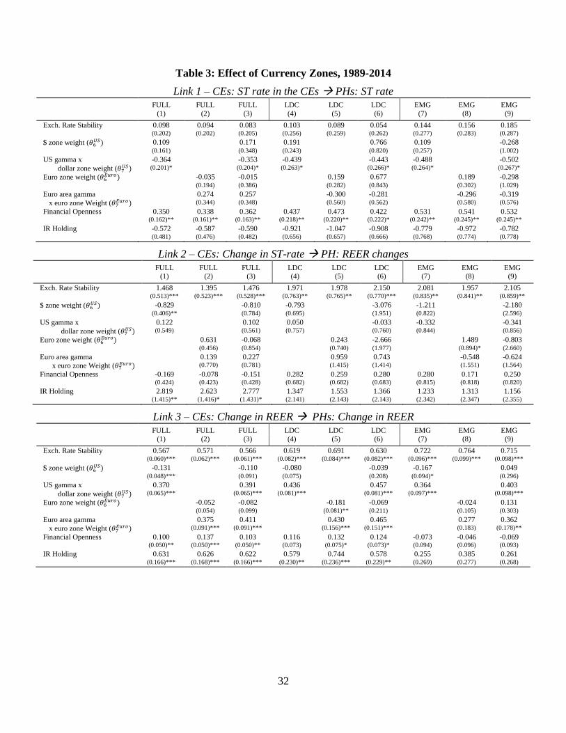
32
Table 3: Effect of Currency Zones, 1989-2014
Link 1 – CEs: ST rate in the CEs PHs: ST rate FULL FULL FULL LDC LDC LDC EMG EMG EMG
(1) (2) (3) (4) (5) (6) (7) (8) (9)
Exch. Rate Stability 0.098 0.094 0.083 0.103 0.089 0.054 0.144 0.156 0.185
(0.202) (0.202) (0.205) (0.256) (0.259) (0.262) (0.277) (0.283) (0.287)
$ zone weight (𝜃6𝑈𝑆) 0.109 0.171 0.191 0.766 0.109 -0.268
(0.161) (0.348) (0.243) (0.820) (0.257) (1.002)
US gamma x -0.364 -0.353 -0.439 -0.443 -0.488 -0.502
dollar zone weight (𝜃7𝑈𝑆) (0.201)* (0.204)* (0.263)* (0.266)* (0.264)* (0.267)*
Euro zone weight (𝜃6𝐸𝑢𝑟𝑜) -0.035 -0.015 0.159 0.677 0.189 -0.298
(0.194) (0.386) (0.282) (0.843) (0.302) (1.029)
Euro area gamma 0.274 0.257 -0.300 -0.281 -0.296 -0.319
x euro zone Weight (𝜃7𝐸𝑢𝑟𝑜) (0.344) (0.348) (0.560) (0.562) (0.580) (0.576)
Financial Openness 0.350 0.338 0.362 0.437 0.473 0.422 0.531 0.541 0.532 (0.162)** (0.161)** (0.163)** (0.218)** (0.220)** (0.222)* (0.242)** (0.245)** (0.245)**
IR Holding -0.572 -0.587 -0.590 -0.921 -1.047 -0.908 -0.779 -0.972 -0.782
(0.481) (0.476) (0.482) (0.656) (0.657) (0.666) (0.768) (0.774) (0.778)
Link 2 – CEs: Change in ST-rate PH: REER changes
FULL FULL FULL LDC LDC LDC EMG EMG EMG (1) (2) (3) (4) (5) (6) (7) (8) (9)
Exch. Rate Stability 1.468 1.395 1.476 1.971 1.978 2.150 2.081 1.957 2.105
(0.513)*** (0.523)*** (0.528)*** (0.763)** (0.765)** (0.770)*** (0.835)** (0.841)** (0.859)**
$ zone weight (𝜃6𝑈𝑆) -0.829 -0.810 -0.793 -3.076 -1.211 -2.180
(0.406)** (0.784) (0.695) (1.951) (0.822) (2.596)
US gamma x 0.122 0.102 0.050 -0.033 -0.332 -0.341
dollar zone weight (𝜃7𝑈𝑆) (0.549) (0.561) (0.757) (0.760) (0.844) (0.856)
Euro zone weight (𝜃6𝐸𝑢𝑟𝑜) 0.631 -0.068 0.243 -2.666 1.489 -0.803
(0.456) (0.854) (0.740) (1.977) (0.894)* (2.660)
Euro area gamma 0.139 0.227 0.959 0.743 -0.548 -0.624
x euro zone Weight (𝜃7𝐸𝑢𝑟𝑜) (0.770) (0.781) (1.415) (1.414) (1.551) (1.564)
Financial Openness -0.169 -0.078 -0.151 0.282 0.259 0.280 0.280 0.171 0.250
(0.424) (0.423) (0.428) (0.682) (0.682) (0.683) (0.815) (0.818) (0.820)
IR Holding 2.819 2.623 2.777 1.347 1.553 1.366 1.233 1.313 1.156
(1.415)** (1.416)* (1.431)* (2.141) (2.143) (2.143) (2.342) (2.347) (2.355)
Link 3 – CEs: Change in REER PHs: Change in REER FULL FULL FULL LDC LDC LDC EMG EMG EMG
(1) (2) (3) (4) (5) (6) (7) (8) (9)
Exch. Rate Stability 0.567 0.571 0.566 0.619 0.691 0.630 0.722 0.764 0.715
(0.060)*** (0.062)*** (0.061)*** (0.082)*** (0.084)*** (0.082)*** (0.096)*** (0.099)*** (0.098)***
$ zone weight (𝜃6𝑈𝑆) -0.131 -0.110 -0.080 -0.039 -0.167 0.049
(0.048)*** (0.091) (0.075) (0.208) (0.094)* (0.296)
US gamma x 0.370 0.391 0.436 0.457 0.364 0.403
dollar zone weight (𝜃7𝑈𝑆) (0.065)*** (0.065)*** (0.081)*** (0.081)*** (0.097)*** (0.098)***
Euro zone weight (𝜃6𝐸𝑢𝑟𝑜) -0.052 -0.082 -0.181 -0.069 -0.024 0.131
(0.054) (0.099) (0.081)** (0.211) (0.105) (0.303)
Euro area gamma 0.375 0.411 0.430 0.465 0.277 0.362
x euro zone Weight (𝜃7𝐸𝑢𝑟𝑜) (0.091)*** (0.091)*** (0.156)*** (0.151)*** (0.183) (0.178)**
Financial Openness 0.100 0.137 0.103 0.116 0.132 0.124 -0.073 -0.046 -0.069 (0.050)** (0.050)*** (0.050)** (0.073) (0.075)* (0.073)* (0.094) (0.096) (0.093)
IR Holding 0.631 0.626 0.622 0.579 0.744 0.578 0.255 0.385 0.261
(0.166)*** (0.168)*** (0.166)*** (0.230)** (0.236)*** (0.229)** (0.269) (0.277) (0.268)

33
Table 3: Continued
Link 4 – CEs: REER changes PHs: EMP FULL FULL FULL LDC LDC LDC EMG EMG EMG
(1) (2) (3) (4) (5) (6) (7) (8) (9)
Exch. Rate Stability -7.891 -6.970 -6.722 -7.551 -7.194 -7.247 -6.989 -6.663 -7.575
(2.118)*** (2.127)*** (2.145)*** (2.182)*** (2.162)*** (2.176)*** (2.622)*** (2.644)** (2.708)***
$ zone weight (𝜃6𝑈𝑆) 0.799 -7.472 -0.210 -4.165 0.302 5.145
(1.704) (3.562)** (2.031) (6.331) (2.377) (8.817)
US gamma x 4.677 3.853 3.590 3.563 5.633 5.574
dollar zone weight (𝜃7𝑈𝑆) (2.117)** (2.133)* (2.179)* (2.159)* (2.416)** (2.435)**
Euro zone weight (𝜃6𝐸𝑢𝑟𝑜) -0.664 -6.715 1.178 -1.653 0.578 7.445
(1.960) (3.907)* (2.224) (6.473) (2.676) (9.079)
Euro area gamma -10.329 -9.768 -9.112 -9.171 -8.532 -8.180
x euro zone Weight (𝜃7𝐸𝑢𝑟𝑜) (3.432)*** (3.468)*** (4.368)** (4.373)** (5.023)* (5.039)
Financial Openness -2.659 -2.124 -2.654 -4.067 -3.931 -3.940 -4.772 -4.357 -4.856 (1.693) (1.667) (1.688) (1.788)** (1.767)** (1.774)** (2.194)** (2.195)** (2.216)**
IR Holding -12.898 -14.236 -12.993 -1.990 -1.886 -2.560 -2.301 -2.519 -2.426
(5.503)** (5.410)*** (5.481)** (5.815) (5.741) (5.765) (7.322) (7.348) (7.395)
Link 5 – CEs: REER changes PH: Stock market price changes
FULL FULL FULL LDC LDC LDC EMG EMG EMG (1) (2) (3) (4) (5) (6) (7) (8) (9)
Exch. Rate Stability -0.089 -0.067 -0.127 0.143 0.099 0.105 0.234 0.112 0.203
(0.164) (0.172) (0.168) (0.229) (0.239) (0.229) (0.277) (0.293) (0.283)
$ zone weight (𝜃6𝑈𝑆) 0.371 0.538 0.538 1.506 0.289 0.676
(0.132)*** (0.249)** (0.201)*** (0.602)** (0.237) (0.856)
US gamma x -1.149 -1.126 -1.521 -1.475 -1.772 -1.705
dollar zone weight (𝜃7𝑈𝑆) (0.160)*** (0.162)*** (0.208)*** (0.208)*** (0.228)*** (0.229)***
Euro zone weight (𝜃6𝐸𝑢𝑟𝑜) -0.079 0.203 -0.193 0.849 -0.021 0.199
(0.155) (0.268) (0.232) (0.604) (0.286) (0.872)
Euro area gamma 0.193 -0.009 0.746 0.540 1.157 0.683
x euro zone Weight (𝜃7𝐸𝑢𝑟𝑜) (0.259) (0.253) (0.451)* (0.433) (0.530)** (0.504)
Financial Openness 0.211 0.097 0.212 0.027 0.010 -0.002 -0.003 0.019 -0.019
(0.135) (0.138) (0.136) (0.179) (0.187) (0.179) (0.215) (0.228) (0.216)
IR Holding -0.610 -0.453 -0.608 -0.530 -0.653 -0.464 -0.427 -0.840 -0.434
(0.388) (0.397) (0.388) (0.531) (0.554) (0.531) (0.703) (0.745) (0.709)
Notes: The estimations are conducted with the robust regression method due to the existence of outliers. * p<0.1; **
p<0.05; *** p<0.01.

34
Table 4: Effects of External Debt
Link 1 CEs: ST rate in the CEs PHs: ST rate Developing Countries (LDC) Emerging Market Countries (EMG)
(1) (2) (3) (4) (5) (6) (7) (8) (9) (10) (11) (12)
Exch. Rate Stability 0.092 -0.185 -0.169 -0.306 -0.272 -0.168 0.206 0.220 0.155 0.116 0.052 0.174
(0.266) (0.381) (0.392) (0.427) (0.383) (0.386) (0.294) (0.427) (0.455) (0.522) (0.427) (0.425) Financial Openness 0.469 0.503 0.509 0.486 0.537 0.508 0.534 0.657 0.659 0.499 0.649 0.658
(0.225)** (0.339) (0.341) (0.373) (0.339) (0.338) (0.253)** (0.381)* (0.380)* (0.445) (0.380)* (0.381)*
IR Holding -0.910 -1.076 -1.069 -1.086 -0.727 -1.136 -0.796 -1.033 -0.995 -0.875 -0.250 -0.981 (0.682) (1.052) (1.047) (1.169) (1.100) (1.080) (0.832) (1.303) (1.318) (1.671) (1.487) (1.313)
External debt -0.004 -0.051
as % exports (0.140) (0.188) External debt -0.049 0.044
as % of GNI (0.376) (0.490) Short-term debt -0.809 -0.754
as % of Exports (0.832) (1.054)
Short-term debt -0.988 -1.089 as % of External debt (1.041) (1.181)
Short-term debt -0.117 0.017
as % of IR (0.293) (0.332)
N 809 532 532 511 532 532 590 377 377 356 377 377 Adj. R2 0.01 -0.00 -0.00 -0.00 0.00 -0.00 0.02 0.00 0.00 -0.01 0.00 0.00
# of countries 63 44 44 44 44 44 39 25 25 25 25 25
Link 2 – CEs: Change in ST-rate PH: REER changes Developing Countries (LDC) Emerging Market Countries (EMG)
(1) (2) (3) (4) (5) (6) (7) (8) (9) (10) (11) (12)
Exch. Rate Stability 2.135 1.977 1.808 2.018 1.838 2.018 2.519 3.693 4.533 3.377 3.306 3.604
(0.782)*** (1.005)* (1.052)* (1.101)* (1.021)* (1.048)* (0.860)*** (1.067)*** (1.177)*** (1.271)*** (1.164)*** (1.059)***
Financial Openness -0.011 -0.595 -0.651 -0.818 -0.648 -0.706 -0.088 -0.607 -0.605 -0.150 -0.056 0.135 (0.692) (0.986) (0.992) (1.021) (0.987) (0.988) (0.845) (1.276) (1.229) (1.397) (1.333) (1.261)
IR Holding 0.969 -1.409 -1.973 -2.718 -1.919 -3.187 1.742 -0.301 2.506 1.112 1.708 -0.215
(2.265) (3.812) (3.909) (4.000) (3.831) (4.129) (2.489) (3.962) (3.903) (4.511) (4.189) (4.084)
External debt -0.579 -1.668
as % exports (0.385) (0.588)***
External debt 0.088 -3.305 as % of GNI (1.028) (1.440)**
Short-term debt -2.611 -3.655
as % of Exports (2.655) (3.373) Short-term debt -0.003 0.901
as % of External debt (3.155) (4.015)
Short-term debt -0.512 -1.397 as % of IR (0.769) (0.864)
N 494 290 290 281 290 290 367 202 202 193 202 202
Adj. R2 0.03 0.01 -0.01 0.00 -0.01 -0.00 0.07 0.09 0.08 0.05 0.03 0.06
# of countries 37 23 23 23 23 23 24 13 13 13 13 13

35
Link 3 – CEs: Change in REER PHs: Change in REER Developing Countries (LDC) Emerging Market Countries (EMG)
(1) (2) (3) (4) (5) (6) (7) (8) (9) (10) (11) (12)
Exch. Rate Stability 0.765 0.601 0.626 0.595 0.599 0.587 0.816 0.913 1.006 0.946 0.902 0.840 (0.084)*** (0.104)*** (0.107)*** (0.112)*** (0.104)*** (0.107)*** (0.099)*** (0.128)*** (0.145)*** (0.148)*** (0.134)*** (0.130)***
Financial Openness 0.155 -0.041 -0.033 -0.049 -0.042 -0.038 -0.063 -0.513 -0.514 -0.546 -0.511 -0.537
(0.074)** (0.102) (0.101) (0.104) (0.101) (0.101) (0.097) (0.153)*** (0.151)*** (0.163)*** (0.153)*** (0.155)***
IR Holding 0.799 0.700 0.757 0.748 0.700 0.771 0.518 0.144 0.332 0.099 0.062 0.411
(0.243)*** (0.394)* (0.398)* (0.406)* (0.391)* (0.422)* (0.286)* (0.474) (0.480) (0.527) (0.482) (0.502)
External debt -0.006 -0.081
as % exports (0.040) (0.070)
External debt -0.096 -0.299
as % of GNI (0.105) (0.177)* Short-term debt -0.116 0.090
as % of Exports (0.270) (0.394)
Short-term debt -0.065 0.403 as % of External debt (0.322) (0.462)
Short-term debt 0.034 0.200
as % of IR (0.079) (0.106)*
N 494 290 290 281 290 290 367 202 202 193 202 202 Adj. R2 0.26 0.31 0.31 0.30 0.31 0.31 0.26 0.36 0.37 0.33 0.34 0.34
# of countries 37 23 23 23 23 23 24 13 13 13 13 13
Link 4 – CEs: REER changes PHs: EMP Developing Countries (LDC) Emerging Market Countries (EMG)
(1) (2) (3) (4) (5) (6) (7) (8) (9) (10) (11) (12)
Exch. Rate Stability -8.347 -9.261 -9.575 -10.517 -9.348 -9.356 -7.367 -12.316 -14.296 -11.545 -8.354 -11.695 (2.265)*** (3.207)*** (3.281)*** (3.550)*** (3.179)*** (3.268)*** (2.741)*** (4.501)*** (4.791)*** (5.273)** (4.426)* (4.430)***
Financial Openness -3.976 -4.116 -4.239 -4.930 -4.666 -4.080 -4.608 -8.189 -7.994 -9.016 -8.115 -7.845
(1.812)** (2.610) (2.627) (2.781)* (2.590)* (2.604) (2.253)** (3.704)** (3.681)** (4.001)** (3.611)** (3.708)**
IR Holding 0.502 7.540 7.410 5.167 6.040 8.156 1.913 13.796 11.415 -6.047 -6.809 14.686
(5.914) (8.918) (8.965) (9.582) (8.933) (9.180) (7.793) (14.168) (14.366) (16.970) (15.415) (14.175)
External debt 0.493 3.526 as % exports (1.140) (1.946)*
External debt 1.115 6.944
as % of GNI (2.975) (4.902) Short-term debt 7.456 18.359
as % of Exports (6.153) (9.249)**
Short-term debt 14.300 37.934 as % of External debt (7.984)* (11.276)***
Short-term debt 0.624 4.277 as % of IR (2.320) (3.241)
N 782 502 502 481 502 502 580 365 365 344 365 365
Adj. R2 0.06 0.07 0.07 0.07 0.07 0.06 0.04 0.06 0.05 0.07 0.09 0.05
# of countries 61 42 42 42 42 42 38 24 24 24 24 24
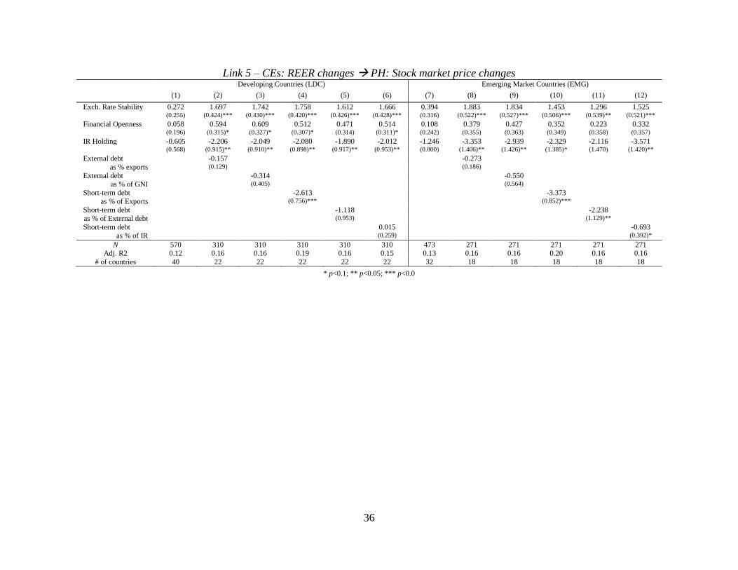
36
Link 5 – CEs: REER changes PH: Stock market price changes Developing Countries (LDC) Emerging Market Countries (EMG)
(1) (2) (3) (4) (5) (6) (7) (8) (9) (10) (11) (12)
Exch. Rate Stability 0.272 1.697 1.742 1.758 1.612 1.666 0.394 1.883 1.834 1.453 1.296 1.525
(0.255) (0.424)*** (0.430)*** (0.420)*** (0.426)*** (0.428)*** (0.316) (0.522)*** (0.527)*** (0.506)*** (0.539)** (0.521)***
Financial Openness 0.058 0.594 0.609 0.512 0.471 0.514 0.108 0.379 0.427 0.352 0.223 0.332
(0.196) (0.315)* (0.327)* (0.307)* (0.314) (0.311)* (0.242) (0.355) (0.363) (0.349) (0.358) (0.357)
IR Holding -0.605 -2.206 -2.049 -2.080 -1.890 -2.012 -1.246 -3.353 -2.939 -2.329 -2.116 -3.571 (0.568) (0.915)** (0.910)** (0.898)** (0.917)** (0.953)** (0.800) (1.406)** (1.426)** (1.385)* (1.470) (1.420)**
External debt -0.157 -0.273
as % exports (0.129) (0.186) External debt -0.314 -0.550
as % of GNI (0.405) (0.564) Short-term debt -2.613 -3.373
as % of Exports (0.756)*** (0.852)***
Short-term debt -1.118 -2.238 as % of External debt (0.953) (1.129)**
Short-term debt 0.015 -0.693
as % of IR (0.259) (0.392)*
N 570 310 310 310 310 310 473 271 271 271 271 271 Adj. R2 0.12 0.16 0.16 0.19 0.16 0.15 0.13 0.16 0.16 0.20 0.16 0.16
# of countries 40 22 22 22 22 22 32 18 18 18 18 18
* p<0.1; ** p<0.05; *** p<0.0

37
Table 5: Effects of External Debt and Currency Weights
Link 1 CEs: ST rate in the CEs PHs: ST rate Developing Countries (LDC) Emerging Market Countries (EMG)
(1) (3) (4) (5) (6) (7) (8) (10) (11) (12) (13) (14)
Exch. Rate Stability 0.092 0.128 -0.235 -0.017 0.500 -0.027 0.206 0.236 -0.125 -0.019 0.502 0.055
(0.266) (0.295) (0.380) (0.340) (0.403) (0.333) (0.294) (0.330) (0.428) (0.444) (0.443) (0.353)
Financial Openness 0.469 0.446 0.625 0.387 0.624 0.548 0.534 0.630 0.712 0.467 0.651 0.509
(0.225)** (0.250)* (0.338)* (0.279) (0.347)* (0.283)* (0.253)** (0.272)** (0.383)* (0.319) (0.350)* (0.298)*
IR Holding -0.910 -0.962 -1.270 -0.927 -0.657 -0.890 -0.796 -0.819 -0.981 -0.494 -0.615 -0.676 (0.682) (0.706) (1.053) (0.760) (1.057) (0.822) (0.832) (0.909) (1.333) (1.042) (1.093) (1.019)
Dollar-denom. Int'l debt(%) -0.267 -0.142
(0.296) (0.348) Dollar share x US gamma -0.224 -0.353
(0.286) (0.288)
Public debt -0.511 -0.236 denominated in USD (%) (0.542) (0.561)
Dollar share (PPG) x US gamma -0.456 -0.801
(0.578) (0.590) Dollar-denom. Int'l debt(%) 0.166 0.050
Financial Inst. (0.276) (0.343)
Dollar share x US gamma -0.714 -0.700 Financial Inst. (0.288)** (0.300)**
Dollar-denom. Int'l debt(%) -0.565 -0.745
Non-Financial Inst. (0.352) (0.389)* Dollar share x US gamma -0.287 -0.399
Non-Financial Inst. (0.314) (0.312)
Dollar-denom. Int'l debt(%)\ 0.030 0.234 Gov't sector (0.359) (0.370)
Dollar share x US gamma -0.161 -0.297
Gov’t Sector (0.330) (0.336)
N 809 565 532 545 429 553 590 445 377 426 372 468
Adj. R2 0.01 0.02 0.00 0.05 0.07 0.00 0.02 0.03 0.01 0.07 0.08 0.01
# of countries 63 40 44 45 35 44 39 29 25 32 28 34
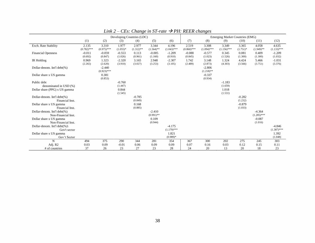
38
Link 2 – CEs: Change in ST-rate PH: REER changes Developing Countries (LDC) Emerging Market Countries (EMG)
(1) (2) (3) (4) (5) (6) (7) (8) (9) (10) (11) (12)
Exch. Rate Stability 2.135 3.310 1.977 2.977 3.344 4.196 2.519 3.308 3.349 3.365 4.058 4.635
(0.782)*** (0.975)*** (1.055)* (1.312)** (1.564)** (1.043)*** (0.860)*** (1.094)*** (1.156)*** (1.751)* (1.949)** (1.133)***
Financial Openness -0.011 -0.059 -0.553 0.113 -0.005 -1.209 -0.088 -0.577 0.345 0.081 0.409 -1.209
(0.692) (0.847) (1.026) (0.961) (1.160) (0.910) (0.845) (1.023) (1.526) (1.300) (1.300) (1.032)
IR Holding 0.969 1.323 -2.320 3.165 2.948 -2.307 1.742 3.148 1.324 4.424 5.466 -1.031 (2.265) (2.620) (3.910) (3.027) (3.253) (3.105) (2.489) (2.873) (4.303) (3.566) (3.751) (3.376)
Dollar-denom. Int'l debt(%) -2.440 -2.806
(0.923)*** (1.218)** Dollar share x US gamma 0.381 -0.337
(0.853) (0.934)
Public debt -0.760 -1.183 denominated in USD (%) (1.447) (1.659)
Dollar share (PPG) x US gamma 0.844 1.018
(1.545) (1.531) Dollar-denom. Int'l debt(%) -0.785 -0.282
Financial Inst. (0.849) (1.232)
Dollar share x US gamma 0.168 -0.879 Financial Inst. (0.885) (1.033)
Dollar-denom. Int'l debt(%) -2.410 -4.364
Non-Financial Inst. (0.991)** (1.285)*** Dollar share x US gamma 0.109 -0.087
Non-Financial Inst. (0.944) (1.016) Dollar-denom. Int'l debt(%)\ -4.175 -4.846
Gov't sector (1.179)*** (1.387)***
Dollar share x US gamma 1.821 1.392 Gov’t Sector (0.989)* (1.048)
N 494 375 290 344 281 354 367 300 202 275 245 303
Adj. R2 0.03 0.09 -0.01 0.06 0.09 0.09 0.07 0.16 0.03 0.12 0.15 0.11
# of countries 37 26 23 27 23 28 24 20 13 20 18 23

39
Link 3 – CEs: Change in REER PHs: Change in REER Developing Countries (LDC) Emerging Market Countries (EMG)
(1) (2) (3) (4) (5) (6) (7) (8) (9) (10) (11) (12)
Exch. Rate Stability 0.765 0.775 0.623 0.823 0.778 0.824 0.816 0.775 0.881 0.881 0.679 0.942
(0.084)*** (0.106)*** (0.106)*** (0.135)*** (0.165)*** (0.115)*** (0.099)*** (0.125)*** (0.132)*** (0.180)*** (0.209)*** (0.125)***
Financial Openness 0.155 0.211 -0.001 0.256 0.185 0.076 -0.063 0.032 -0.445 0.154 0.145 -0.048
(0.074)** (0.092)** (0.103) (0.099)*** (0.122) (0.100) (0.097) (0.117) (0.174)** (0.134) (0.139) (0.113)
IR Holding 0.799 0.799 0.575 1.193 1.062 0.172 0.518 0.733 0.025 1.293 1.062 -0.187 (0.243)*** (0.285)*** (0.394) (0.312)*** (0.342)*** (0.343) (0.286)* (0.329)** (0.491) (0.368)*** (0.402)*** (0.371)
Dollar-denom. Int'l debt(%) -0.083 0.049
(0.100) (0.140)
Dollar share x US gamma 0.082 0.018
(0.093) (0.107) Public debt -0.231 -0.171
denominated in USD (%) (0.146) (0.189)
Dollar share (PPG) x US gamma 0.457 0.198 (0.156)*** (0.175)
Dollar-denom. Int'l debt(%) 0.039 0.172
Financial Inst. (0.087) (0.127) Dollar share x US gamma 0.247 0.173
Financial Inst. (0.091)*** (0.106)
Dollar-denom. Int'l debt(%) -0.065 -0.132 Non-Financial Inst. (0.104) (0.138)
Dollar share x US gamma 0.218 0.137
Non-Financial Inst. (0.099)** (0.109) Dollar-denom. Int'l debt(%)\ 0.010 -0.082
Gov't sector (0.130) (0.152)
Dollar share x US gamma 0.391 0.355 Gov’t Sector (0.109)*** (0.115)***
N 494 375 290 344 281 354 367 300 202 275 245 303
Adj. R2 0.26 0.23 0.32 0.28 0.29 0.27 0.26 0.23 0.34 0.25 0.23 0.29
# of countries 37 26 23 27 23 28 24 20 13 20 18 23
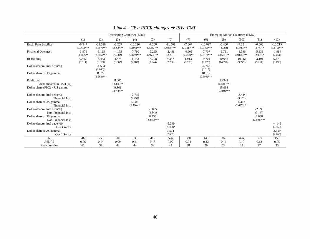
40
Link 4 – CEs: REER changes PHs: EMP
Developing Countries (LDC) Emerging Market Countries (EMG)
(1) (2) (3) (4) (5) (6) (7) (8) (9) (10) (11) (12)
Exch. Rate Stability -8.347 -12.528 -8.209 -10.216 -7.208 -11.561 -7.367 -10.027 -5.480 -9.224 -6.663 -10.215
(2.265)*** (2.697)*** (3.200)** (3.191)*** (3.332)** (2.828)*** (2.741)*** (3.049)*** (4.588) (3.988)** (3.747)* (3.119)***
Financial Openness -3.976 -8.195 -4.175 -7.780 -5.295 -2.498 -4.608 -7.707 -8.731 -8.596 -5.339 -1.994
(1.812)** (2.216)*** (2.582) (2.427)*** (2.660)** (2.261) (2.253)** (2.517)*** (3.671)** (2.878)*** (2.837)* (2.454)
IR Holding 0.502 -4.443 4.874 -6.133 -8.708 9.357 1.913 -9.704 10.046 -10.066 -3.191 9.671 (5.914) (6.829) (8.862) (7.182) (8.544) (7.230) (7.793) (8.825) (14.228) (9.749) (9.261) (9.196)
Dollar-denom. Int'l debt(%) -4.504 -4.748
(2.646)* (3.315)
Dollar share x US gamma 8.029 10.819
(2.562)*** (2.694)*** Public debt 8.605 13.941
denominated in USD (%) (4.275)** (5.545)**
Dollar share (PPG) x US gamma 9.801 15.993 (4.780)** (5.869)***
Dollar-denom. Int'l debt(%) -2.715 -3.444
Financial Inst. (2.431) (3.151) Dollar share x US gamma 6.085 8.412
Financial Inst. (2.520)** (2.687)***
Dollar-denom. Int'l debt(%) -0.895 -2.899 Non-Financial Inst. (2.642) (3.117)
Dollar share x US gamma 8.736 9.630
Non-Financial Inst. (2.455)*** (2.601)*** Dollar-denom. Int'l debt(%)\ -5.349 -4.146
Gov't sector (2.803)* (2.958)
Dollar share x US gamma 3.514 3.959 Gov’t Sector (2.687) (2.765)
N 782 550 502 530 415 526 580 445 365 426 373 459
Adj. R2 0.06 0.14 0.09 0.11 0.13 0.09 0.04 0.12 0.11 0.10 0.12 0.05
# of countries 61 39 42 44 33 42 38 29 24 32 27 33

41
Link 5 – CEs: REER changes PH: Stock market price changes Developing Countries (LDC) Emerging Market Countries (EMG)
(1) (2) (3) (4) (5) (6) (7) (8) (9) (10) (11) (12)
Exch. Rate Stability 0.272 0.033 1.198 -0.268 -0.184 0.358 0.394 0.136 1.170 -0.268 -0.118 0.247
(0.255) (0.256) (0.424)*** (0.288) (0.354) (0.330) (0.316) (0.304) (0.504)** (0.356) (0.387) (0.361)
Financial Openness 0.058 0.331 0.263 0.369 0.300 -0.008 0.108 0.379 0.130 0.293 0.220 0.027
(0.196) (0.210) (0.310) (0.224) (0.271) (0.246) (0.242) (0.237) (0.356) (0.262) (0.280) (0.260)
IR Holding -0.605 -0.650 -1.884 -0.591 -1.614 -1.522 -1.246 -1.611 -3.202 -1.458 -1.467 -2.164 (0.568) (0.599) (0.892)** (0.597) (0.873)* (0.742)** (0.800) (0.805)** (1.358)** (0.855)* (0.924) (0.966)**
Dollar-denom. Int'l debt(%) 0.830 1.032
(0.258)*** (0.325)***
Dollar share x US gamma -1.448 -1.622
(0.231)*** (0.249)*** Public debt -0.256 -0.392
denominated in USD (%) (0.475) (0.498)
Dollar share (PPG) x US gamma -1.916 -1.857 (0.491)*** (0.503)***
Dollar-denom. Int'l debt(%) 0.571 0.619
Financial Inst. (0.218)*** (0.285)** Dollar share x US gamma -1.407 -1.618
Financial Inst. (0.217)*** (0.236)***
Dollar-denom. Int'l debt(%) 0.256 0.283 Non-Financial Inst. (0.258) (0.297)
Dollar share x US gamma -1.752 -1.792
Non-Financial Inst. (0.245)*** (0.253)*** Dollar-denom. Int'l debt(%)\ 0.847 0.893
Gov't sector (0.279)*** (0.304)***
Dollar share x US gamma -1.463 -1.438 Gov’t Sector (0.282)*** (0.289)***
N 570 470 310 451 374 423 473 401 271 391 350 381
Adj. R2 0.12 0.24 0.21 0.25 0.28 0.22 0.13 0.27 0.20 0.27 0.28 0.24
# of countries 40 33 22 36 27 31 32 27 18 29 25 27
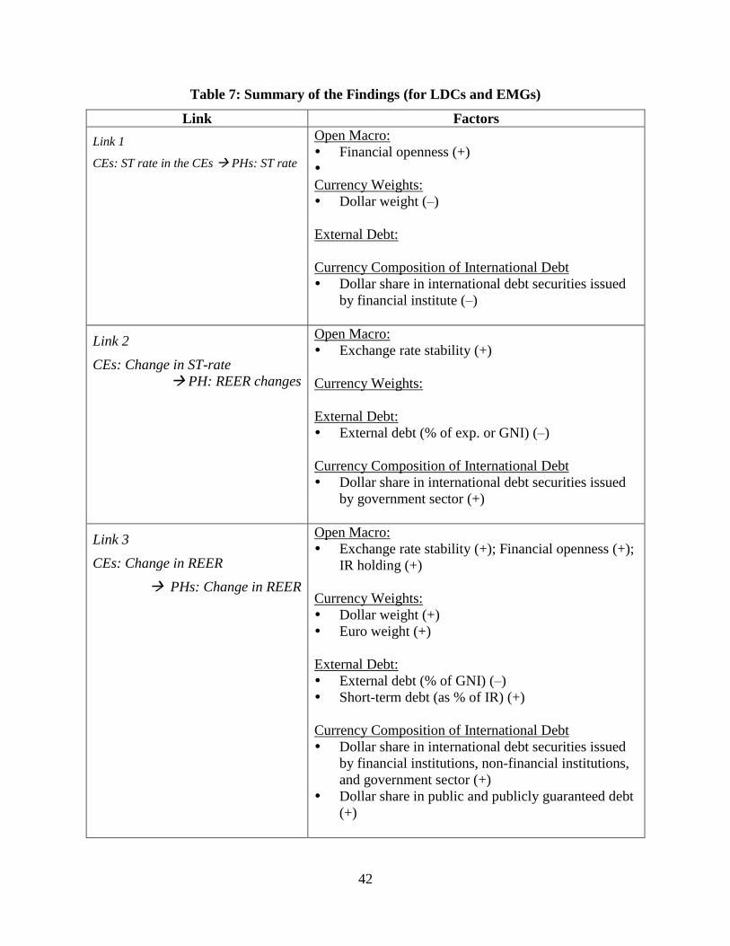
42
Table 7: Summary of the Findings (for LDCs and EMGs)
Link Factors
Link 1
CEs: ST rate in the CEs PHs: ST rate
Open Macro:
Financial openness (+)
Currency Weights:
Dollar weight (–)
External Debt:
Currency Composition of International Debt
Dollar share in international debt securities issued
by financial institute (–)
Link 2
CEs: Change in ST-rate
PH: REER changes
Open Macro:
Exchange rate stability (+)
Currency Weights:
External Debt:
External debt (% of exp. or GNI) (–)
Currency Composition of International Debt
Dollar share in international debt securities issued
by government sector (+)
Link 3
CEs: Change in REER
PHs: Change in REER
Open Macro:
Exchange rate stability (+); Financial openness (+);
IR holding (+)
Currency Weights:
Dollar weight (+)
Euro weight (+)
External Debt:
External debt (% of GNI) (–)
Short-term debt (as % of IR) (+)
Currency Composition of International Debt
Dollar share in international debt securities issued
by financial institutions, non-financial institutions,
and government sector (+)
Dollar share in public and publicly guaranteed debt
(+)
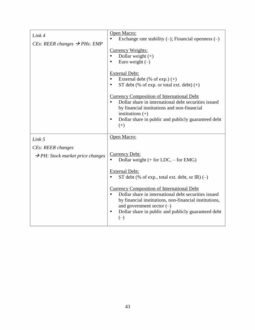
43
Link 4
CEs: REER changes PHs: EMP
Open Macro:
Exchange rate stability (–); Financial openness (–)
Currency Weights:
Dollar weight (+)
Euro weight (–)
External Debt:
External debt (% of exp.) (+)
ST debt (% of exp. or total ext. debt) (+)
Currency Composition of International Debt
Dollar share in international debt securities issued
by financial institutions and non-financial
institutions (+)
Dollar share in public and publicly guaranteed debt
(+)
Link 5
CEs: REER changes
PH: Stock market price changes
Open Macro:
Currency Debt:
Dollar weight (+ for LDC, – for EMG)
External Debt:
ST debt (% of exp., total ext. debt, or IR) (–)
Currency Composition of International Debt
Dollar share in international debt securities issued
by financial institutions, non-financial institutions,
and government sector (–)
Dollar share in public and publicly guaranteed debt
(–)

44
Figure 1: Five Paths of Linkage
US, Euro, Japan(CEs)
Peripheral Economies (PHs)
ST-rate ST-rate
Stock Market
REER REER
EMP EMP
Link 1
Link 3
Link 5
Link 4
Link 2

45
Figure 2: Proportion of Significant F-Tests
(i) CE: Policy Interest Rate PH: Policy Interest Rate
(ii) CE: Policy Interest Rate PH: REER
(iii) CE: REER PH: REER
0.2
.4.6
.81
% o
f S
ig. E
stim
ate
s
1992-19941995-1997
1998-20002001-2003
2004-20062007-2009
2010-20122013-2014
IDC Sample
Real Global Fin. Global
Cross-link
0.2
.4.6
.81
% o
f S
ig. E
stim
ate
s
1992-19941995-1997
1998-20002001-2003
2004-20062007-2009
2010-20122013-2014
LDC Sample
Real Global Fin. Global
Cross-link
0.2
.4.6
.81
% o
f S
ig. E
stim
ate
s
1992-19941995-1997
1998-20002001-2003
2004-20062007-2009
2010-20122013-2014
IDC Sample
Real Global Fin. Global
Cross-link
0.2
.4.6
.81
% o
f S
ig. E
stim
ate
s
1992-19941995-1997
1998-20002001-2003
2004-20062007-2009
2010-20122013-2014
IDC Sample
Real Global Fin. Global
Cross-link
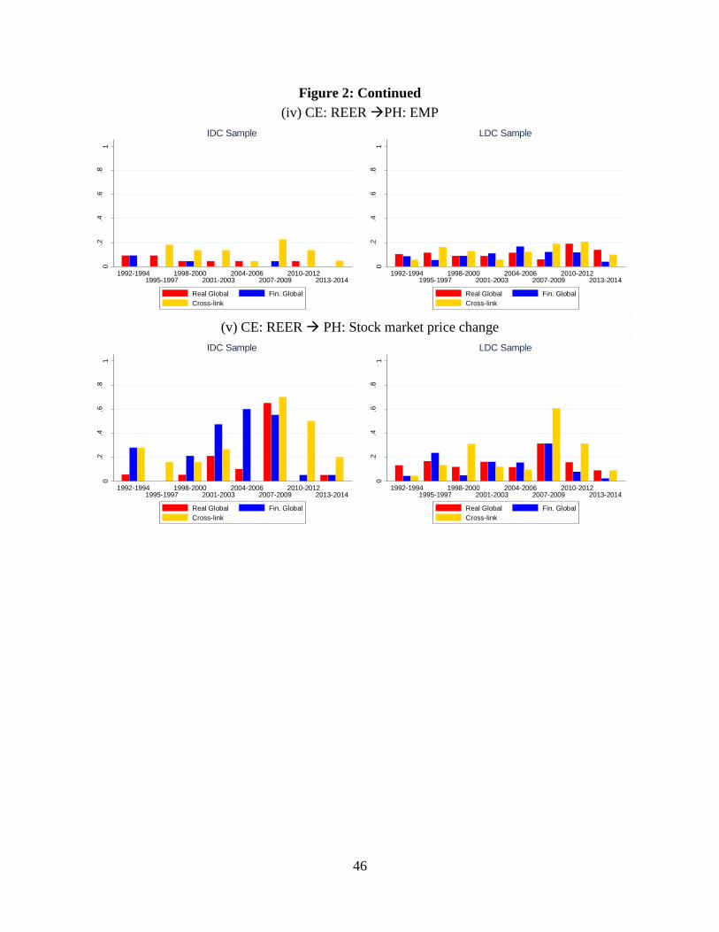
46
Figure 2: Continued
(iv) CE: REER PH: EMP
(v) CE: REER PH: Stock market price change
0.2
.4.6
.81
% o
f S
ig. E
stim
ate
s
1992-19941995-1997
1998-20002001-2003
2004-20062007-2009
2010-20122013-2014
IDC Sample
Real Global Fin. Global
Cross-link
0.2
.4.6
.81
% o
f S
ig. E
stim
ate
s
1992-19941995-1997
1998-20002001-2003
2004-20062007-2009
2010-20122013-2014
LDC Sample
Real Global Fin. Global
Cross-link
0.2
.4.6
.81
% o
f S
ig. E
stim
ate
s
1992-19941995-1997
1998-20002001-2003
2004-20062007-2009
2010-20122013-2014
IDC Sample
Real Global Fin. Global
Cross-link
0.2
.4.6
.81
% o
f S
ig. E
stim
ate
s
1992-19941995-1997
1998-20002001-2003
2004-20062007-2009
2010-20122013-2014
LDC Sample
Real Global Fin. Global
Cross-link

47
Figure 3: Proportion of Significant ��’s
(i) CE: Policy Interest Rate PH: Policy Interest Rate
(ii) CE: Policy Interest Rate PH: REER
(iii) CE: REER PH: REER
0.2
.4.6
.81
% o
f S
ig. E
stim
ate
s
1992-19941995-1997
1998-20002001-2003
2004-20062007-2009
2010-20122013-2014
LDC
U.S. Japan
Euro
0.2
.4.6
.81
% o
f S
ig. E
stim
ate
s
1992-19941995-1997
1998-20002001-2003
2004-20062007-2009
2010-20122013-2014
EMG
U.S. Japan
Euro
0.2
.4.6
.81
% o
f S
ig. E
stim
ate
s
1992-19941995-1997
1998-20002001-2003
2004-20062007-2009
2010-20122013-2014
LDC
U.S. Japan
Euro
0.2
.4.6
.81
% o
f S
ig. E
stim
ate
s
1992-19941995-1997
1998-20002001-2003
2004-20062007-2009
2010-20122013-2014
EMG
U.S. Japan
Euro
0.2
.4.6
.81
% o
f S
ig. E
stim
ate
s
1992-19941995-1997
1998-20002001-2003
2004-20062007-2009
2010-20122013-2014
LDC
U.S. Japan
Euro
0.2
.4.6
.81
% o
f S
ig. E
stim
ate
s
1992-19941995-1997
1998-20002001-2003
2004-20062007-2009
2010-20122013-2014
EMG
U.S. Japan
Euro
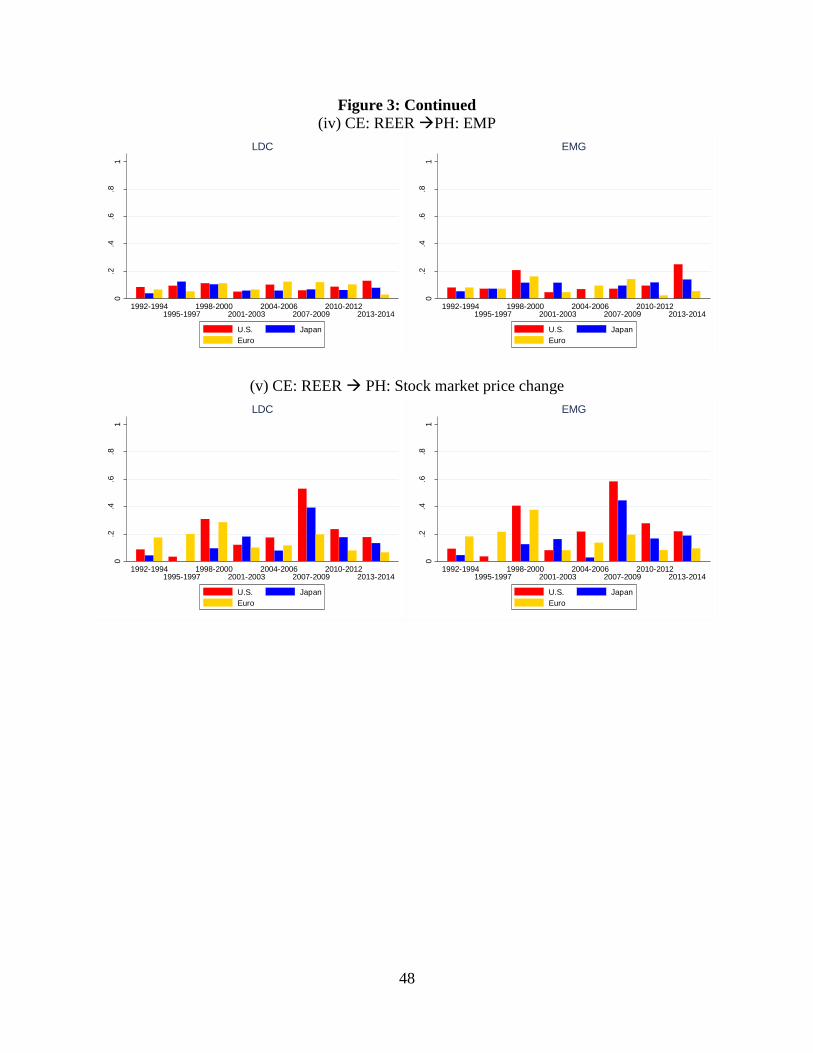
48
Figure 3: Continued
(iv) CE: REER PH: EMP
(v) CE: REER PH: Stock market price change
0.2
.4.6
.81
% o
f S
ig. E
stim
ate
s
1992-19941995-1997
1998-20002001-2003
2004-20062007-2009
2010-20122013-2014
LDC
U.S. Japan
Euro
0.2
.4.6
.81
% o
f S
ig. E
stim
ate
s
1992-19941995-1997
1998-20002001-2003
2004-20062007-2009
2010-20122013-2014
EMG
U.S. Japan
Euro
0.2
.4.6
.81
% o
f S
ig. E
stim
ate
s
1992-19941995-1997
1998-20002001-2003
2004-20062007-2009
2010-20122013-2014
LDC
U.S. Japan
Euro
0.2
.4.6
.81
% o
f S
ig. E
stim
ate
s
1992-19941995-1997
1998-20002001-2003
2004-20062007-2009
2010-20122013-2014
EMG
U.S. Japan
Euro

49