sensors

Article

On Data-Driven Sparse Sensing and LinearEstimation of Fluid Flows

Balaji Jayaraman *,† and S. M. Abdullah Al Mamun

School of Mechanical and Aerospace Engineering, Oklahoma State University, Stillwater, OK 74078, USA;smamun@ostatemail.okstate.edu* Correspondence: jayaramanbalaji@gmail.com† Currently at SciAI LLC.

Received: 9 May 2020; Accepted: 26 June 2020; Published: 4 July 2020�����������������

Abstract: The reconstruction of fine-scale information from sparse data measured at irregularlocations is often needed in many diverse applications, including numerous instances of practicalfluid dynamics observed in natural environments. This need is driven by tasks such as dataassimilation or the recovery of fine-scale knowledge including models from limited data. Sparsereconstruction is inherently badly represented when formulated as a linear estimation problem.Therefore, the most successful linear estimation approaches are better represented by recoveringthe full state on an encoded low-dimensional basis that effectively spans the data. Commonly usedlow-dimensional spaces include those characterized by orthogonal Fourier and data-driven properorthogonal decomposition (POD) modes. This article deals with the use of linear estimation methodswhen one encounters a non-orthogonal basis. As a representative thought example, we focus onlinear estimation using a basis from shallow extreme learning machine (ELM) autoencoder networksthat are easy to learn but non-orthogonal and which certainly do not parsimoniously represent thedata, thus requiring numerous sensors for effective reconstruction. In this paper, we present anefficient and robust framework for sparse data-driven sensor placement and the consequent recoveryof the higher-resolution field of basis vectors. The performance improvements are illustrated throughexamples of fluid flows with varying complexity and benchmarked against well-known POD-basedsparse recovery methods.

Keywords: sparse reconstruction; extreme learning machines; sensors; SVD; POD; compressivesensing

1. Introduction

The challenge of multiscale flow sensing lies in the use of fewer sensors than there arescales. Therefore, deciphering the true multiscale behavior of the system is often accomplishedthrough post-processing. In the case of simulations, the sensor (grid points) budgets are limited bycomputational considerations; therefore, it is necessary to resort to coarse-grained models which inturn are expected to produce nearly accurate outcomes as full-resolution models. Such a situation iscommonly encountered in atmospheric turbulence sensing closer to the surface—in a region calledthe atmospheric boundary layer—where simulation-based research [1,2] has served as a key enablerfor the extraction of the explainable knowledge of coherent structures and underlying mechanisms.In recent times, a major driver for the direct measurement of atmospheric turbulence data has beenthe use of swarms of unmanned vehicles [3,4] flying in the atmosphere, whose capability to extractthe wind velocity vectors [5,6] and turbulent statistics of the atmospheric boundary layer [7] havebeen demonstrated using simulations. This current numerical exploration from our group is one steptowards the ultimate goal of the sparse sensing of turbulent fields using unstructured measurements

Sensors 2020, 20, 3752; doi:10.3390/s20133752 www.mdpi.com/journal/sensors

Sensors 2020, 20, 3752 2 of 31

within large flow fields leveraging unmanned aerial vehicle dynamics. In such practical situationsas those discussed above, measurement data represent the absolute truth and are often acquiredfrom very few probes, limiting their in-depth analysis. A common recourse is to combine such sparsemeasurements with physics-based priors, either in the form of idealized simulations (data assimilation),phenomenology or knowledge of a sparse basis to recover detailed information (sparse recovery).

A second example arises from situations (e.g., computational simulations) in which the data areoften in surplus and consequently offer the best avenue for the in-depth analysis of realistic flowsdue to the high density of computational grid probes. With the growth in computing power and theresulting ability to generate big data, it is easy to recognize the need for rapid low-dimensional analysistools [8–12] and evolutionary models [12–16] and regenerate the high-dimensional state withouta significant loss of information [17]. Thus, tools for encoding information into a low-dimensionalfeature space complement sparse recovery tools that decode compressed information. This, in essence,is a key aspect of leveraging machine learning for fluid flow analysis [18,19] and broadly speaking fothe recovery of coarse-grained information [20].

This work focuses on the algorithmic aspects of recovering a high-dimensional field from sparsedata through data-informed sensor placement for accurate reconstruction of the full system statein situations such as those listed above. Although their deployment in practical settings is notdemonstrated here, the underlying principles are expected to guide users of the technology.

Regarding related work on linear estimation in the basis space, at a conceptual level, sparserecovery is deeply connected to compressive sensing (CS) [21–24] which has made it possible todirectly sample [18] data in real-time without having to collect high-resolution information andthen perform downsampling. Of course, in the case of direct sampling, the recovery algorithmneeds a generic or data-driven basis in which the data are sparse. The recovery of fine-scaleinformation from sparse data has been gaining traction in various manifestations including gappyproper orthogonal decomposition (GPOD) [25,26], Fourier-based compressive sensing (CS) [21–24]and Gaussian kernel-based kriging [27–29]. A tangential application of such ideas is in the accelerationof nonlinear model order reduction using sparse sampling for hyper-reduction [30–33]. Sparserecovery techniques such as GPOD [25,26,30] utilize the knowledge of the POD basis computedoffline from the data ensemble to recast the reconstruction problem in the feature space and solveit using least-squares minimization approaches. Derivatives [25,27,30,34] of this approach includean iterative formulation [25,27,30,34] to successively approximate the POD basis in the event thatthe low-dimensional basis is not known a priori. Nevertheless, these iterative approaches remainimpractical on account of their limited accuracy and computational cost.

While data-driven POD-based approaches can optimally represent the data, they do not generalizewell. Therefore, their use in practice requires a priori knowledge of the basis vectors. One way toovercome this stringent requirement is to adopt computational simulations of the twin dynamicalsystem or model simulations to build the basis library. Nevertheless, such methods find tremendousvalue in data-driven modeling (machine learning, Koopman operator models [13,35]) applications andthe nonlinear model order reduction [10] of systems that are statistically stationary.

Alternatively, one can use a generic basis such as Fourier or wavelets that may not always beeffective at dimensionality reduction on a data-driven basis, especially for inhomogeneous fluid flowphenomena with multiple scales and sharp gradients. The resulting higher-dimensional feature spacerequires more sensors for accurate reconstruction. Consequently, such flow systems are invariablyunder-sampled during sensing, partially due to the algorithm. To recover the higher-dimensionalstate, the best sparse solution is often sought instead of a least-squares estimate that overfits to theundersampled data. The success of compressive sensing (CS) [21–24] lies in achieving this usingl1-norm regularized least-squares reconstruction.

Sparsity-promoting l1 regularized reconstruction can also be combined with a data-driven PODbasis, such as in the reconstruction of sparse flow fields from particle image velocimetry (PIV) data [18]

Sensors 2020, 20, 3752 3 of 31

and pressure measurements around a cylinder surface [19]. Thus the choice of basis has an impact onalgorithmic design.

Regarding sensor placement and sparse recovery, in addition to the choice of the basis space andits relationship with the inversion algorithm, the choice of sparse measurement locations impactssparse recovery. The sparse measurement locations determine what information pertaining to thephysical system is collected and in turn determines the quality of the sparse recovery. In general,identifying “optimal” sensing locations for spatio-temporal fields is an NP-hard problem and an opentopic of research. However, greedy smart sampling methods have been reported in the literaturesuch as using extrema of POD-basis vectors [36,37], hyperreduction approaches such as DEIM forsensing [31,38] and objective-based matrix condition number minimization (or maximization, as thecase may be) using both explicit [26,39] and submatrix volume maximization using QR-pivoting [40].All these methods have primarily been employed with simulation or experimental (using particleimage velocimetry (PIV)) data, where the distributed information of the field is available to identifysensor placement. In addition, there is a vast amount of interesting literature on the greedy sensingof network dynamics with discrete events where extreme event detection, such as faults, is required;for example, water [41–43] or communication networks. Given that the interest in this paper is“super-resolution” or the sparse recovery of continuous fields from sparse measurements, we focus ontechniques such as DEIM and QR-pivoting-based matrix conditioning.

Contribution of This Work

In this article, we explore the use of an arbitrary data-driven basis for sensor placement and sparserecovery applications. Such situations may be encountered in machine learning applications wherebasis spaces that do not optimally span the data may be readily available from other stages of thedata science workflow. An example of such a basis is the modes from dynamic mode decomposition(DMD) [35] or projections available in extreme learning machine (ELM)-based autoencoders [44–46],among others. Such DMD and ELM modes are known to be non-orthogonal, unlike POD-modes,and their suitability for data-driven sensor placement/sparse recovery has not been explored toour knowledge. Further, the arbitrary non-orthogonal basis suffers from a lack of parsimony forlow-dimensional representation and a lack of inherent hierarchy, resulting in larger sensor budgets,inaccurate reconstruction, ineffective sensor placement due to basis non-orthogonality and theenhanced complexity of the inverse problem solution. To this end, we develop a framework thatcombines the Gram–Schmidt orthogonalization of the arbitrary data-driven basis with well knownmethods for data-driven sensor placement and linear sparse estimation.

We systematically analyze the accuracy of this integrated sparse reconstruction (SR) frameworkby comparing it with the corresponding POD-based SR—a standard approach for the linear sparseestimation of fluid flows. The analysis focuses on comparing the basis structure, the basis dimensionfor a chosen representation accuracy, the basis hierarchy for the chosen datasets and the interplay ofSR accuracy with sensor budget and placement. In particular, the effect of sensor placement on sparserecovery has barely been explored in the literature and provides an insight into the practical limitationsof sparse recovery design. In this way, the current effort builds on our earlier research [47,48] thatcharacterized this interplay. For this study, we chose two use cases to demonstrate the methods: alow-dimensional cylinder wake flow at a laminar Reynolds number (Re = 100) and higher dimensionalsea surface temperature field from NOAA.

The rest of manuscript is organized as follows. In Section 2, we review the basics of sparsereconstruction theory and different choices of data-driven bases including POD and ELM. Section 3discusses the role of measurement locations and reviews the approaches for data-driven sensorplacement. In Sections 4 and 6, we summarize the different algorithms employed for SR and trainingdata generation. Section 7 compares the structure of the different data-driven bases, while Section 8compares their performance for the different use cases. We summarize the major conclusions from thisstudy in Section 9.

Sensors 2020, 20, 3752 4 of 31

2. Recovering Resolved Fields from Sparse Data Using Linear Estimation

For certain high-resolution data of fluid flow at any particular instant, x ∈ RN , the correspondingsparse representation may be written as x ∈ RP with P� N. Then, the sparse reconstruction problemis to recover x given x along with information of the sensor locations in the form of the measurementmatrix C ∈ RP×N as

x = Cx. (1)

Often, in practice, it is only the sensor locations that are available; therefore, an imaginaryreconstruction grid may be designed to suit the desired end goals. In this way, the measurement matrixC shows how the sparse data x (of dimension P) are downsampled from better-resolved sensor data,x (of dimension N). In this article, we focus on vectors x that have a sparse representation in a basisspace Φ ∈ RN×K such that K � N and yielding x = Φa. Naturally, the recovery of lost information isnever absolute, as the reconstruction problem is ill-posed; i.e., there are more unknowns than equationsin Equation (1), which rules out least-squares solutions such as x = C+ x.

2.1. Sparse Reconstruction Theory

Sparse reconstruction has theoretical foundations in inverse problem frameworks [49] appliedto diverse fields such as geophysics [50,51] and image processing [52]. Many signals tend to be“compressible” or sparse in some K-sparse bases Φ; i.e.,

x =Nb

∑i=1

φiai or x = Φa, (2)

where Φ ∈ RN×Nb and a ∈ RNb with K significant or non-zero elements. In general, K is not knowna priori for an unknown system with only sparse data available. Further, it is not always obviouswhich K of the Nb basis vectors φi results in the most accurate reconstruction. A prudent and commonapproach is to adopt a more exhaustive basis set of dimension Nb ≈ P > K for a desired K, all of whichwill be naturally smaller than the dimension N of the full-field data, and then to search for the optimalK-sparse solution. In practice, it makes sense to have K, Nb � N, especially if the choice of basis isoptimal, such as for data-driven POD modes. Therefore, the choice of Φ, K, N and Nb represents theoverall problem design. While standard image compression techniques (with transform coding inJPEG and JPEG-2000 compression standards [53]) adopt a sample-and-then-compress approach—i.e.,they collect a high-resolution sample, transform it to a Fourier or wavelet basis space and retainonly a suitable K-sparse structure—techniques such as compressive sensing [21,23,54–56] and sparsereconstruction [12,17,26,39,48] directly infer the K-sparse coefficients by essentially combining thesteps in Equations (1) and (2) as below:

x = CΦa = Θa, (3)

where Θ ∈ RP×Nb relates the basis coefficients a in the feature space and the sparse data x in thephysical space. The challenge of recovering x from the underdetermined system in Equation (1) arisesfrom C being ill-conditioned and N � P. However, when x is sparse in Φ, the recovery of a ∈ RK

using Equation (3) becomes feasible as K ∼ P; that is, solving for K unknowns (in a) using P constraints(x), as per Equation (6). Commonly, the s-norm regularized least squares error s is minimized, which ischosen appropriately to recover x as per Equation (2). The l2-regularized method estimates a such thatthe expression in Equation (4) is minimized.

‖x−Θa‖22 + λ‖a‖2

2. (4)

The exact expression for a uses the left pesudo-inverse of Θ, as given in Equation (4),

Sensors 2020, 20, 3752 5 of 31

a = (Θ)+ x, (5)

where Θ+ =(ΘTΘ + λI

)−1ΘT x . This regularized least-squares approach is nearly identical to the

GPOD algorithm of Everson and Sirovich [30] when Φ is the POD basis. However, X in GPOD containszeros as placeholders for all the missing elements, whereas the above formulation retains only themeasured data points. A possible method to enhance the sparsity of the resulting a is to minimize‖a′‖0; i.e., minimize the number of non-zero elements such that Θa′ = x. It has been shown [57] thatP = K+ 1 (P > K in general) independent measurements are sufficient to recover the sparse coefficientswith high probability using l0 reconstruction. On the other hand, when employing P ≤ K independentmeasurements, the probability of recovering the sparse solution is diminished. Compressedsensing [58–61] overcomes the computational difficulties with NP-complex l0-reconstruction usingl1 methods that guarantee the near-exact recovery of K-sparse coefficients. The reconstruction ofl1 is a relatively simple convex optimization problem as compared to l0 and solvable using linearprogramming techniques such as basis pursuit [21,54,62], shrinkage [63] and sequential thresholdedleast-squares approaches [64]. These different methods solve the constrained reconstruction problemin Equation (6) with complexity O(N3) for Nb ≈ N at the cost of needing P > O(Klog(Nb/K))measurements [21,54,58] to exactly reconstruct the K-sparse vectors.

l1 reconstruction : a = min ‖a′‖1 such that Θa′ = x

l1 cost function to minimize : min ‖x−Θa‖22 + λ‖a‖1

(6)

As reported in prior efforts [47,48], the interplay between the design choices of Nb, K, P and the choiceof algorithm are non-trivial and impact the reconstruction quality. For clarity, Nb is the candidatebasis dimension, meaning that Nb / N and K is the desired system reconstruction dimension, whichdetermines the best possible sparse recovery quality; P is the available sensor budget. Often, P ≥ Kis required for reasonably accurate sparse recovery. In addition to the sensor budget, the sensorplacement also plays an important role as it is tied to the structure of individual basis functions in Φ todetermine the condition of Θ. Therefore, it makes sense to ensure the sensor–basis vector relationshiphelps improve the sparse recovery quality. Often, this involves placing sensors in such a way that themeasurement basis (rows of C) is incoherent with the data basis Φ. Smart sensor placement strategiesprovide a more structured approach by taking into account the underlying physics and coherence ofthe data.

2.2. Computation of Data-Driven Basis

Given the central role that basis choice plays in the sparse recovery of continuous fields, especiallywith limited data, it is important to consider φis that are customized to the data. Among otherfactors, such as the carrying signatures of the physical phenomena, this also results in a parsimoniousrepresentation of the data. In fact, it has been shown [18] that the data-driven POD basis outperformsthe generic cosine basis when performing reconstruction with small amounts of data, while theaccuracy becomes comparable with more data. In this work, we explore two classes of data-drivenspaces, namely POD and extreme learning machine (ELM) bases, with POD-based SR serving as abenchmark for data-driven SR.

Proper Orthogonal Decomposition (POD) Basis

Proper orthogonal decomposition (POD) is a popular approach for dimensionality reduction.The POD modes are computed from the eigendecomposition of the symmetric, positive, definitetwo-point spatial (or temporal) correlation tensor of the data snapshots. The appropriately scaledeigenvectors represent the singular vectors or POD modes in space or time—as the case may be—for agiven dataset. These POD modes or singular vectors form an orthogonal basis that optimally representsthe data snapshots in terms of the least-squares approach. Therefore, the detailed flow field can be

Sensors 2020, 20, 3752 6 of 31

reconstructed using only a few (relative to the system state dimension) coefficients; therefore, this isattractive for dimensionality reduction. Obviously, not all systems have a fast decaying singularvalue spectrum; therefore, the extent of dimension reduction is problem-dependent. Given that fluidmechanics problems typically have a much larger state dimension than the number of snapshots(N � M), the POD problem is reformulated as the eigendecomposition of the two-point temporalcorrelation tensor of dimension M×M [65]. Denoting the full state data snapshots as X ∈ RN×M

(different from x ∈ RN) where N, M are the state and snapshot dimensions, the symmetric temporalcorrelation matrix CM ∈ RM×M (Equation (7)) can be built and the eigendecomposition performed asshown in Equation (8).

CM = XTX. (7)

CMV = VΛ. (8)

where V = [v1, v2, . . . , vM] represent the eigenvectors and the diagonal elements of Λ denote theeigenvalues [λ1, λ2, . . . , λM]. . The POD/singular value decomposition (SVD) modes Φ and coefficientsa (for the linear expansion as shown in Equation (2)) can then be estimated as per Equations (9) and (10).

Φ = XV√

Λ−1. (9)

a = ΦTX. (10)

The method of snapshots limits the maximum number of POD basis vectors to M, which is typicallysmaller than the dimension of full state vectors, N. Further dimension reduction may be achievedusing singular value thresholding such that K < M modes are retained.

2.3. ELM Autoencoder Basis

In this paper, we explore methods for dealing with unconventional data-driven bases that arecommonly encountered in sparse data-driven modeling. For example, it is not uncommon to adoptradial basis functions (RBFs) to generate continuous representations of discrete measurements due totheir suitability for representing a wide variety of unknown flow physics [11]. In this work, we leveragebases generated from extreme learning machines (ELMs) [44,45]—a class of shallow neural networkregressors employing a Gaussian prior that was used as encoder–decoder maps for a given data set byZhou et al. [46,66,67]. The ELM-autoencoder is a single hidden-layer feedforward neural network(SLFN) with randomized projection followed by the Gaussian activation of the data onto hidden nodesand a linear map to the output (the same as the input). By setting the number of hidden nodes to asmall fraction of the input/output feature dimension, we generate sparse representations of the state,as shown in Figure 1. Given snapshots of data X ∈ RN×M (or simply xj ∈ RN for j = 1 . . . M), we relatethe full state data to a K-dimensional feature space vector using the ELM autoencoder, as shown belowin Figure 1 and Equation (11).

xj =K

∑i=1

φiaji =

K

∑i=1

φihi(xj) =K

∑i=1

φig(wTi xj + bi) (11)

where xj ∈ RN is a snapshot of the input data with j as the snapshot index, wi ∈ RN is the randominput weight vector, bi is the random bias, g(.) is the activation function (chosen as the Gaussian;i.e., g(z) = e−(z

2)) operating on the linearly transformed input state to yield and hi and φi ∈ RN

(Φ ∈ RN×K) are the weights that map hidden layer features to the output. In matrix form, the linearEquation (11) can be written as in Equation (12), where a is the matrix of outputs (with elements aj

i)

Sensors 2020, 20, 3752 7 of 31

from the hidden layer and h(xj) = [h1(xj), · · · , hk(xj)] = [aj1, · · · , aj

k], which represents the outputcorresponding to the input snapshot xj.

Figure 1. Schematic of the extreme learning machine (ELM) autoencoder network. In this architecture,the output features are the same as input features.

X = Φa; a =

a11 · · · a1

k...

. . ....

aM1 · · · aM

k )

T

=

h(x1)...

h(xM)

T

=

h1(x1) · · · hk(x1)...

. . ....

h1(xM) · · · hk(xM)

T

(12)

The output weights in matrix form for a given X are shown in Equation (13).

X =

x11 · · · x1

N...

. . ....

xM1 · · · xM

N

T

; Φ =

φ11 · · · φN

1...

. . ....

φ1k · · · φN

k

T

(13)

Using Equation (12), Φ is estimated in a least squares sense as in Equation (14).

Φtrain = Φ = Xa+ = Xa+train (14)

The columns of Φ represent the ELM-basis, and the density of the hidden layer determines theeffective system dimension. However, a major drawback of this basis is the lack of orthogonality.It is well known that orthogonal bases yield parsimonious representations of the data as comparedto their non-orthogonal counterparts, therefore requiring fewer sensors for a similar reconstructionquality [47]. In addition, basis orthogonality is useful for data-driven sensor placement using methodssuch as discrete empirical interpolation method (DEIM) [31]. To this end, we extend the ELM basisgeneration with a Gram–Schmidt procedure (Algorithm 1) to generate an orthogonal ΦELM−GS whichspans more or less the same subspace as ΦELM. This particular step represents a one-time cost but canresult in greatly improved properties for sparse recovery, as will be seen from the results presented inthe later sections.

Sensors 2020, 20, 3752 8 of 31

Algorithm 1: Gram–Schmidt Orthogonalization of ELM Basis (ELM-GS)input :N dimensional non-orthogonal basis [φ1,φ2,. . . ,φK]output :N dimensional orthogonal basis [φorth

1 ,φorth2 ,. . . ,φorth

K ]

1 Define the projection: Π(φ, φorth) =

⟨φorth, φ

⟩⟨φorth, φorth

⟩2 for k = 1 to K do3 if k = 1 then4 φOrth

k = φ1;5 else6 φOrth

k = φk - ∑k−1j=1 Π(φ, φorth)φk

7 end8 end

3. Sensor Placement, Data Basis and Incoherence

It is well known that recovery quality is tied to sensor placement (structure of measurementmatrix, C), budget and the choice of basis, Φ [48]. Specifically, the sensor placement needs to beincoherent with respect to the low-dimensional basis Φ [23], and this is usually accomplished byusing a randomized measurement matrix for Φ. In this study, we restrict ourselves to single-pixelmeasurements with C of the form C← [e$1 , e$2 , . . . , e$p ]

T , where e$p is column vector with zeros anda value of one at the sensor index p. The purpose of making C (Equations (1)–(3)) incoherent withrespect to the basis Φ is to ensure that the measurements distributed in space excite the different modesand ensure CΦ is not rank-deficient. This is usually quantified in terms of the coherency number, µ, asshown in Equation (15) [68],

µ(C, Φ) =√

N · maxi≤P, j≤K

∣∣〈ci, Φj〉∣∣ , (15)

where ci is a row vector in C (i.e., ci = e$j ) and φj is a column vector of Φ. µ which typically ranges from1 (incoherent) to

√N (coherent). The smaller the µ, the fewer measurements are needed to reconstruct

the data. There are many metrics that can be leveraged for improving sensor placement. However,identifying a truly optimal sensor arrangement is combinatorially hard and therefore an active areaof research. There is a current search for greedy sensor placement algorithms with near-optimalperformance by leveraging a variety of optimization surrogates [26,37,69,70]. In the context of flowreconstruction, sensor placement can be viewed as a problem of identifying and activating only afew rows of the basis matrix Φ such that the matrix Θ (for P = K = Nb) or its variants M = ΘTΘ orM = ΘΘT (depending on if P > K = Nb or P < K = Nb respectively) have low condition numbers,as schematically illustrated in Figure 2.

Figure 2. Schematic illustration of sparse sensor placement. The pastel-colored rectangles representrows activated by the sensors denoted in the measurement matrix through dark squares.

In this study, we consider two different greedy approaches for nearly optimal sensor placement insparse recovery applications, namely the discrete empirical interpolation method (DEIM) [31,71] and

Sensors 2020, 20, 3752 9 of 31

reduced matrix QR-factorization with column pivoting [40] instead of choosing sensors at randomlocations within the region. These approaches are summarized below for completeness.

The most simple and efficient sensor placement strategy is to sample at random locations bychoosing the first P values from a random permutation of the entire sensor array of dimension N.Several ideas can also be adopted, such as K-means clustering, as was used in [12].

Sensors generated from the pivot matrix in QR factorization (with column pivoting) are designedto minimize the condition number of the matrix Θ or M = ΘΘT to improve the full state recovery.Specifically, the reduced matrix QR factorization [72] decomposes any given real matrix A ∈ RS×T

with a full column rank into a unitary matrix Q ∈ RS×T and an upper triangular matrix R ∈ RT×T .QR factorization with column pivoting yields AD = QR, with D ∈ RT×T being a square columnpermutation matrix containing ones and zeros such that the diagonal values of R , rii form a decreasingsequence. Therefore, choosing the first P columns of A and first P rows of D maximizes the determinantof the submatrix AD for a given budget P. Given that the measurement matrix C selects columnsof ΦT (or rows of Φ) and interpreting AD as ΘT = ΦTCT , the connection between the permutationmatrix D and the measurement matrix C can be directly observed. Using C = DT ensures that thesubmatrix volume of Θ is maximized and its condition number minimized. We refer the reader to thework presented in [40,48] for a more detailed discussion of the algorithm.

In contrast, the discrete empirical interpolation method (DEIM) [31,71] iteratively tests the lineardependence of the columns of Θ = CΦ to identify each sensor location. Here, we identify interpolationpoints (with indices $j) with the most linear dependence error relative to previously determinedinterpolation points. The primary idea behind DEIM is to estimate a high-dimensional state usinginformation at sparsely sampled interpolation points which can be adopted for sensor placement insparse recovery. While the sequence of input bases is not critical for the QR-pivoting based approach,it is important for DEIM. Therefore, the sensor placement will depend on basis choice. Secondly,the orthogonality of the basis ensures the interpolation indices are hierarchical and non-repeating.Therefore, the sensor placement methods are not as effective with non-orthogonal bases.

4. Sparse Recovery Algorithm

In addition to basis generation and data-driven sensor placement, the choice of linear estimationapproaches is also critical (Section 2.1). This choice depends on the combination of sensor budgetand basis dimension. In this work, we adopt the l2 sparse reconstruction (summarized throughEquations (3) and (4)) with K ≤ M basis vectors (Φ), which is also the dimension of the featurevector a. Least-squares reconstruction demands the candidate basis dimension, Nb, be the same as K,the reconstruction dimension. The naming convention adopted is as follows: xj ∈ RN denotes theinstantaneous jth full flow state with the entire dataset of M snapshots denoted by X ∈ RN×M. Thealgorithm used in this work applies to both single and batch-style reconstruction in series and parallel.

One can construct the measurement matrix—i.e., C ∈ RN×N or C ∈ RP×N—depending on thedimension of the sparse data vector; that is, whether xj ∈ RN or RP. In this work, we consistently usethe high-dimensional version of xj which is similar to the earlier work on gappy POD methods [30].For high-resolution data xj ∈ RN with a chosen basis of φk ∈ RN , the low-dimensional features,aj ∈ RK, are obtained as per Equation (16). We also define the masked (incomplete) data xj ∈ RN ,corresponding measurement matrix C ∈ RN×N and mask vector m ∈ RN . Since the GPOD resultsin a larger measurement matrix (N × N ) with numerous rows of zeros, the mask vector (containing1s and 0s) bypasses the added computational complexity by operating on xj through a point-wisemultiplication operator < · >; i.e., xj =< mj · xj >, where each element of xj multiplies with thecorresponding element of mj. This compact representation allows the mj to be different for eachsnapshot if desired.

xj =K

∑k=1

φkajk; xj =< m · xj >= Cxj. (16)

Sensors 2020, 20, 3752 10 of 31

In SR, we recover the full data from the masked data given in Equation (17) by estimating thecoefficients aj (in the l2 sense) with the basis φk generated offline. As the masked basis vectors are notnecessarily orthogonal, the coefficient vector aj is approximated by minimizing the least-squares errorEj (Equation (18)).

xj ≈ mK

∑k=1

ajkφk. (17)

Ej =

∣∣∣∣∣∣∣∣∣∣xj −m

K

∑k=1

ajkφk

∣∣∣∣∣∣∣∣∣∣2

2

=∣∣∣∣∣∣xj −m · Φaj

∣∣∣∣∣∣22=∣∣∣∣∣∣xj − CΦaj

∣∣∣∣∣∣22=

∣∣∣∣∣∣∣∣∣∣xj −

K

∑k=1

ajkφk

∣∣∣∣∣∣∣∣∣∣2

2

. (18)

where m is multiplied point-wise with each column of Φ to yield φk. The above formulation is validfor a case in which the measurement locations are static. In the case of the dynamically evolving sensorplacement, the mask vector mj changes with every snapshot xj for j = 1..M. The error Ej representsthe individual snapshot reconstruction error that is be minimized to estimate the features aj. It is easilyseen that one has to minimize the different Ejs separately to estimate the entire coefficient matrix,a ∈ RK×M for the entire batch of snapshots. In the above formulation, Φ is analogous to CΦ = Θ inEquation (3).

To minimize Ej, its derivative is computed with respect to aj resulting in the normal equation given

by Maj = f j where Mk1,k2 = 〈φk1, φk2〉 or M = ΦTΦ and f jk = 〈xj, φk〉 or f j = ΦT xj. The recovered

solution is given by xSRj =

K∑

k=1φk aj

k.

4.1. Sequential Thresholding for l1 Regularized Least Squares

Two situations commonly need to be handled: (i) a case with very few sensors—i.e., P �Nb—requiring the effective recovery dimension K to be smaller than the candidate basis dimension Nb;or (ii) a case in which the candidate basis has no inherent ordering—a key enabler for incrementallybetter reconstruction. In both situations mentioned above, the algorithm needs to be able to identifythe K-best coefficients a for sparse recovery, which in turn requires sparsity-promoting l1 normminimization reconstruction as given by Equation (6) . In this work, we adopt an iterative sequentialleast-squares thresholding framework to extend the least-squares algorithm used above, and this ispresented in Algorithm 2. The idea here is to repeatedly “shrink” the least-squares coefficients using athreshold hyperparameter.

Sensors 2020, 20, 3752 11 of 31

Algorithm 2: l1-based algorithm: Sparse reconstruction with known basis, Φ.

input :Full data ensemble X ∈ RN×M

Incomplete data X ∈ RN×M

The mask vector m ∈ RN .The chosen sparsity Ksparse

output :Approximated full data X ∈ RN×M

1 Compute masked basis function: Φ = mΦ, where Φ ∈ RN×K f ull

2 Initial guess for Coefficients a = pinv(Φ) ∗ X, where a ∈ RK f ull×M

3 Set a tolerance ε4 while ‖anew − aold‖2 > ε do5 for each snapshot index j ≤ M do6 Create a row vector λ where λj = kth

sparse highest value fromabsolute(aj);

7 end8 for j ≤ M do9 for each element in aj index i ≤ K f ull do

10 if aji < λj then

11 Put aji = 0 ;

12 Remove ith column from Φ;13 end14 end15 aj(places of non zero elements) = pinv(Φ) ∗ xj ;16 end17 anew = a ;18 end19 Approximated full data x = Φ ∗ anew

5. Algorithmic Complexity

In this brief section, we present the algorithmic complexity of the above methods. Computingthe POD basis requires O(N×M2) operations, where N, M are the full state and snapshot dimensions,respectively. The subsequent cost of sparse recovery is O(N× K×M) for both methods, where K ≤ M isthe desired recovery dimension. In practical flows with a low-dimensional structure, POD is expectedto result in a smaller K than other classes of a data-driven basis. This helps limit the sensor budget andreconstruction cost. Further, since the snapshot dimension (M) is tied to the basis dimension (K), the largerthe K, the more snapshots (of dimension M) are needed, resulting in a higher computational cost.

The complexity of sensor placement depends on the method chosen. For example,QR factorization with column pivoting requires O(N3) operations for an N × N matrix and O(NM2)

for an N ×M matrix. The DEIM method involves a complexity of O(NM3) when retaining M PODmodes and identifying M sensors with a full state dimension of N. These estimates are consistent withour experience of deploying DEIM and QR-pivoting approaches on the datasets reported in this work.

6. Sparse Recovery Use Cases

To demonstrate the performance of sparse recovery using the ELM-GS basis for different sensorplacements, we consider two representative flow fields, namely a low-dimensional cylinder wakeflow and a more complex geophysical field of sea surface temperature data from NOAA. The SRperformance using ELM-GS basis is compared with that of POD-based SR.

6.1. Low-Dimensional Cylinder Wake Flow

As the first use case, we consider the data-driven sparse reconstruction of the cylinder wakeflow fields at a Reynolds number of Re = 100 involving unsteady wake dynamics (see Figure 3).

Sensors 2020, 20, 3752 12 of 31

The two-dimensional flow data is modeled using a higher-order spectral Galerkin framework [73]Nektar++ to capture the vortex roll-up process and eddying structure. Specifically, we adopt a fourthorder spectral expansion within each element to solve the incompressible Naiver–Stokes equations,

∇ · u = 0, (19a)

∂u∂t

+ u · ∇u = −∇P/ρ + ν∇2u, (19b)

where u and v are horizontal and vertical velocity components, P is the pressure field and ν is the fluidviscosity. The simulation domain used extends over−25D ≤ x ≤ 45D and−20D ≤ y ≤ 20D, where Dis the diameter of the cylinder. To reduce the state dimension, we consider a reduced domain of extent−2D ≤ x ≤ 10D and −3D ≤ y ≤ 3D that encompasses the key flow dynamics. The resulting statedimension is ∼24,000 for each variable, and data snapshots are recorded every ∆t = 0.2. The meshdistribution ensures that the thin shear layers near the surface are resolved, as is the transient wake physics.

The time-evolution of the cylinder wake flow (Figure 3) shows the wake instability and limit-cycledynamics (Figure 4). The rapid decay of the singular value spectrum (Figure 5) clearly shows that thesystem evolves in a low-dimensional space. In this study, we use 300 snapshots collected (every 0.2non-dimensional time units) over 60 non-dimensional times, T = Ut

D which represents ∼10 cycles ofthe dynamics.

(a) T = 25 (b) T = 68 (c) T = 200

Figure 3. Isocontour plots of the stream-wise velocity component for the cylinder flow atRe = 100 at T = 25, 68, 200, showing the evolution of the flow field. Here, T represents the timenon-dimensionalized by the advection time-scale.

(a) 2D view (b) 3D view

Figure 4. The temporal evolution of the first three normalized proper orthogonal decomposition (POD)coefficients for the limit cycle cylinder flow at Re = 100.

Sensors 2020, 20, 3752 13 of 31

Figure 5. Singular value spectrum of the data matrix for both the cylinder wake flow at Re = 100 andthe sea surface temperature(SST) data.

6.2. Global Sea Surface Temperature (SST) Data

Representing a more complicated use case for the methods presented in this article, the sea surfacetemperature (SST) dataset represents synoptic-scale ocean turbulence and is made available by theNational Oceanic & Atmospheric Administration (NOAA) (https://www.esrl.noaa.gov/psd/).

The data represent a filtered turbulent field as they represent the daily mean temperature fromhigh-resolution blended analysis for the year 2018. The dataset includes daily snapshots (for 365 days)of a temperature field with a spatial resolution of 0.25◦ longitude × 0.25◦ latitude, resulting in a totalstate dimension of 720× 1440. Of this full state dimension of 1,036,800 observations, only 691,150(≈ 69%) measurements correspond to non-landed regions and are used here. The singular value spectra(Figure 5) for this dataset shows a slow decay of eigenvalues as compared to the low-dimensional wakeflow and is therefore higher dimensional. In spite of the turbulent nature of this data, the dynamics ofthe POD features in Figure 6 show nearly periodic evolution at the large scales.

(a) Temporal evolution of POD features (b) Phase plot

Figure 6. The temporal evolution of the first three normalized POD coefficients for the sea surfacetemperature (SST) data.

7. Assessment of Dimensionality, Basis Structure and Hierarchy for Sparse Recovery

7.1. Dimensionality

Data-driven bases vary in their capacity to represent full state information as quantified throughthe number of basis vectors of a given basis set to represent the full state up to a desired accuracy;i.e., the system dimensionality in a given basis space. For a POD basis that is energy-optimal, theknowledge of the singular value spectrum (Equation (8)) precisely informs us of the energy content in

each mode and also allows for characterization of the cumulative energy, EK =K∑

k=1

λk(λ1+λ2+···+λM)

× 100

as retained in the reconstruction up to a desired mode K. For the low-dimensional limit cycle wakedynamics at Re = 100, two and five POD modes (of the 300 basis vectors computed) are requiredto capture 95% and 99% of the energy content (variance), respectively. We also compute errPOD

K =

Sensors 2020, 20, 3752 14 of 31

∣∣∣∣X−ΦPODK×N aPOD

K×M

∣∣∣∣2, where ΦPOD

K×N , aPODK×M represents the matrix comprising K POD vectors and the

corresponding coefficients for the different snapshots, respectively. Relating the system dimension withenergy from the singular value spectrum and reconstruction error offers a way to compare differentbases that may be “ordered” and “unordered” in some way.

In such situations, characterizing the system dimension K through the reconstruction error(with respect to the true data) offers a way forward. For example, in the case of ELM, the trainingerror from the ELM network (Equation (14)) may be used. The error is quantified according to theFrobenius norms denoted by errELM

K =∣∣∣∣X− XELM

K

∣∣∣∣2 and errELM−GS

K =∣∣∣∣∣∣X− XELM−GS

K

∣∣∣∣∣∣2

using

the K-modal reconstruction of the flow fields, XELMK = ΦELM

train,K×N aELMtrain,K×M = ΦELM

K×N aELMK×M and

XELM−GSK = ΦELM−GS

train,K×N aELM−GStrain,K×M = ΦELM−GS

K×N aELM−GSK×M , respectively. A simple method of estimating

the system dimension in any basis is to compare the reconstruction error with the correspondingPOD-based reconstruction which optimally captures the variance in the data. Figure 7 shows thecomparison of the decay of representation errors with dimension for the different bases, and Table 1quantifies the dimension corresponding to 95% and 99% energy in terms of POD singular value spectra.We clearly see from Figure 7a that the POD basis offers the most parsimonious representation of thedata (K95 = 2, K99 = 5), followed by ELM-GS (K95 = 6, K99 = 7) and ELM (K95 = 16, K99 = 19).The corresponding values for the high-dimensional SST data are also tabulated. The ELM-GS is onlyslightly more expensive than POD (Figure 7b), although it spans nearly the same subspace as theELM basis.

(a) ELM; ELM-GS; POD (Cylinder) (b) ELM-GS; POD (Cylinder)

(c) ELM; ELM-GS; POD (SST) (d) ELM-GS; POD (SST)

Figure 7. Reconstruction error (errPODK , errELM

K , errELM−GSK ) decay using different numbers of bases

(K) for POD, ELM and Gram–Schmidt extreme learning machine (ELM-GS) bases, considering bothcylinder wake data (top row) and sea surface temperature (SST) data (bottom row).

Sensors 2020, 20, 3752 15 of 31

Table 1. Dimension estimation (K95 and K99) for POD, ELM and ELM-GS corresponding to 95% and99% energy using a POD reconstruction for both cylinder wake and sea surface temperature (SST) data.

Case Basis

POD ELM ELM-GS

Cylinder K95 2 16 5K99 5 19 7

SST K95 9 92 16K99 66 195 83

7.2. Basis Structure

Having compared the dimension of the data in different basis subspaces, we also look at thetopology of the basis vectors. In Figure 8, we compare the first six modes for the POD, ELM andELM-GS for the cylinder wake flow. The well-known orthogonal structure of the POD basis for thecylinder wake contrasts with the qualitative similar structure of the ELM modes (modes 1–3 and5–6 are similar to each other), while that of the ELM-GS displays a tendency to transition from theELM modal structure to the orthogonal POD modal structure with increasingly smaller eddies at thehigher modes. This semblance of scale hierarchy of the ELM-GS modes contributes to their ability toaccurately represent data using fewer modes. We quantify the basis orthogonality using the productΦTΦ for both ELM and ELM-GS in Figure 9. These plots show clear diagonal dominance for theELM-GS basis.

7.3. Basis Hierarchy

For a given dataset , the generated POD modes offer built-in ordering; i.e., one can sequentiallyinclude more modes to generate increasingly accurate representations of the true data. This is notlikely the case for non-optimal basis choices such as Fourier or ELM bases. Here, we explore thisaspect of the basis hierarchy for ELM and ELM-GS bases in comparison to that of POD modes byincrementally adding basis vectors to recover the flow field while tracking the error decrease in thereconstructed field. Outcomes from this analysis are presented in Figure 10 for both the chosen datasets.We clearly observe that both ELM-GS and POD show a systematic decrease of the reconstruction errorwith an increase in the number of basis vectors, K, and the error decay is rapid for low-dimensionalreconstruction; in contrast, for the ELM basis, we clearly see a non-monotonic error decay, althoughthe overall trend shows an error decrease as expected. These trends are verified for the multiple choicerandom initialization of the weights in the ELM training, as denoted by the seed β. The outcomesclearly show that ELM-GS introduces a consistent basis hierarchy independent of the ELM trainingand is therefore a robust choice for sparse recovery applications.

Sensors 2020, 20, 3752 16 of 31

(a) POD Mode-1 (b) ELM Mode-1 (c) ELM-GS Mode-1

(d) POD Mode-2 (e) ELM Mode-2 (f) ELM-GS Mode-2

(g) POD Mode-3 (h) ELM Mode-3 (i) ELM-GS Mode-3

(j) POD Mode-4 (k) ELM Mode-4 (l) ELM-GS Mode-4

(m) POD Mode-5 (n) ELM Mode-5 (o) ELM-GS Mode-5

(p) POD Mode-6 (q) ELM Mode-6 (r) ELM-GS Mode-6

Figure 8. Comparison of the first six modes of POD, ELM and ELM-GS. The POD and ELM-GS sharesimilar structures, possibly due to their underlying orthogonality, while ELM represents repeatingstructures not unlike POD modes 1 and 2.

(a) ELM (SST) (b) ELM-GS (SST) (c) ELM (Cylinder)

0.1

0.2

0.3

0.4

0.5

0.6

0.7

0.8

0.9

(d) ELM-GS (Cylinder)

Figure 9. ΦTΦ contour plot of ELM and ELM-GS basis for both cylinder wake and sea surfacetemperature (SST) data. Red indicates a value of one, and blue indicates a value of zero.

Sensors 2020, 20, 3752 17 of 31

(a) POD (Cylinder) (b) POD (SST)

(c) ELM (Cylinder) (d) ELM (SST)

(e) ELM-GS (Cylinder) (f) ELM-GS (SST)

Figure 10. Plots showing how the error decays with the increase of basis number for all three casesPOD, ELM and ELM-GS for both cylinder wake data (left column) and sea surface temperature (SST)data (right column). For ELM and ELM-GS, the different realizations corresponding to the differentrandom seeds used for the network weights in the ELM (SLFN) training are shown, as well as theaverage error over 20 different training samples.

8. Assessment of Sparse Reconstruction Performance

8.1. Sparse Reconstruction Experiments, Analysis Methods and Error Quantifications

Having explored the ability of the different basis spaces to approximate the data, we now assesstheir linear sparse estimation performance using multiple sensor placement strategies. To accomplishthis, we reconstruct the full field from sparse data using numerically simulated flow fields andobservation datasets (NOAA-SST). In the offline stage, the full field representation is used to learnthe data-driven basis and sensor locations. In practice, the sensor locations are identified using priorknowledge of the system. The concept of data-driven sensor placement is adopted here with the aimof identifying choices that provide robust outcomes with accuracy. In this study, we design sensorsas fixed (in time) single-point measurements using random or smart sampling algorithms such asDEIM or QR-factorization with column pivoting. This offline step yields at most M bases (M is the

Sensors 2020, 20, 3752 18 of 31

number of snapshots) for use in the reconstruction process in Equation (2) (candidate basis dimensionof Nb = M) and P (desired) sensor locations. The desired recovery dimension K can be chosen as Nbor smaller (K < Nb). The earlier discussion from Section 2 and prior studies [48] shows us that, for achosen K, P ≥ K is likely to generate reasonable results using l2 reconstruction with K = Nb. If Nb islarge, the best subset of K bases is generally chosen to generate an accurate reconstruction by lookingfor a K-sparse solution using l1 methods. If the basis vectors are ordered in terms of their “relevance”to this dataset, then the best subset of K-bases will also be the first K-bases of the sequence. We use thisas a way to verify the basis hierarchy in POD and ELM-GS by comparing the outcomes from l1 (withM = Nb > K) and l2 (with Nb = K) methods. Once the basis hierarchy is established, we evaluatethe reconstruction performance by comparing the true flow field with those from SR using POD andELM-GS bases for an ensemble of numerical experiments spread over different sensor budgets, P, andreconstructed system dimensions, K, using l2 methods.

Assessing the accuracy of the sparse recovery outcomes across a wide range of design parametersis challenging. For example, two POD modes may generate the same reconstruction accuracy asfive ELM-GS modes, as shown in Table 1. Further, two different flows may have different scaleseparations and therefore dimensionality in a basis space. To address this, we first define the variousnormalized metrics for the comparison and generalization of outcomes as used in our earlier work [47,48]. We recount these briefly for completeness.

To illustrate these ideas, we note that two POD modes capture 95% of the energy for the cylinderwake flow (KPOD

95 = 2) while the SST data require nine modes (KPOD95 = 9). Therefore, analysis

across different flow regimes and algorithms requires thenormalization of the system dimension asK∗ = K/K95 and a normalized sensor budget, P∗ = P/K95, to be handled. Using this, we design anensemble of sparse recovery experiments in the normalized P∗ − K∗ space over the range 1 < K∗ < 6and 1 < P∗ < 12 for the different choices of bases and sensor placements. The lower bound of oneaspect is chosen so that the minimally accurate reconstruction captures 95% of the energy—this choiceis left to the user. To quantify the flow field recovery performance for the different problem designs,we define the mean squared reconstruction error as

εSRK∗ ,P∗ =

1M

1N

M

∑j=1

N

∑i=1

(Xi,j − XSRi,j )

2, (20)

where X is the true data and XSR is the recovered field using sparse measurements; N and M representthe state and snapshot dimensions affiliated with indices i and j, respectively. We also define the meansquared errors εFR

K∗95and εFR

K∗ for the full reconstruction (FR) using the different bases; namely, POD andELM-based SR are

εFRK∗95

=1M

1N

M

∑j=1

N

∑i=1

(Xi,j − XFR,K∗95i,j )2; εFR

K∗ =1M

1N

M

∑j=1

N

∑i=1

(Xi,j − XFR,K∗i,j )2, (21)

where XFR is the reconstruction using exact coefficients for the different bases, K∗95 = K95/K95 = 1 isthe normalized system dimension corresponding to 95% energy capture and K∗ = K/K95 representsthe desired reconstructed system dimension. Therefore, the FR errors represent the best case values;i.e., lower bounds for the sparse recovery errors. This enables us to define normalized error metricsrepresenting the absolute (ε1) and relative (ε2) measures as

ε1 =εSR

K∗ ,P∗

εFRK∗95

, ε2 =εSR

K∗ ,P∗

εFRK∗

. (22)

These normalized metrics allow us to compare both the “absolute” and relative reconstructionquality for a given problem design (i.e., P, K). While ε1 represents the SR error normalized bythe corresponding full reconstruction error for 95% energy capture, ε2 represents the relative SRperformance obtained by normalizing the SR error with the FR error for the desired reconstruction

Sensors 2020, 20, 3752 19 of 31

accuracy (for dimension K). These normalized metrics enable us to compare the different SRalgorithms/design choices across different flow regimes.

8.2. Basis Hierarchy in ELM-GS and POD Bases

We have shown through the decay of reconstruction errors in Section 7.3 that POD and ELM-GSbases have inherent hierarchical structures for flow recovery. Here, we establish the same by comparinga K-sparse recovery of high-resolution data from heavily downsampled data using both l2 and l1minimization approaches. For these experiments using the cylinder wake flow data, we build a candidatebasis library of dimension 200 from which the desired sparse solution is estimated using DEIM-basedsparse measurements. DEIM-based sensing is attractive due to its computational efficiency and theability to identify physically relevant sensor locations. In Figure 11, we compare the reconstructedinstantaneous flow field and estimated sparse coefficients with the corresponding ground truth for acase with P∗ = 18, K∗ = 9. For both the POD and ELM-GS basis, we see that l1 minimization using thesequential thresholded least squares (Section 4.1) excite only the first few coefficients (Figure 11a,c), similarto l2 minimization, thereby verifying that the bases are ordered in terms of their relevance to the data.Leveraging this outcome, we pursue the rest of this analysis using least-squares minimization methods.

(a) POD (l1) (b) POD (l1)

(c) ELM-GS (l1) (d) ELM-GS (l1)

Figure 11. Normalized projected and reconstructed coefficient a ((a) and (c)) and The line contourcomparison of the streamwise velocity between the actual CFD solution field (blue) and theenergy-based SR reconstruction (red) using the l1 SR algorithm for both POD and ELM-GS-basedreconstruction ((b) and (d)) at K∗ = 9, P∗ = 18.

8.3. Comparison of Sensor Placement Using ELM-GS and POD Bases

Using knowledge of the underlying data-driven bases, data/physics-informed sensor placementcan be determined, as discussed in Section 3; this can in turn be used for sparse recovery. In this study,we use both ELM-GS and POD bases to identify smart sensors, as shown in Figure 12 for the cylinderwake flow and SST data. The red dots in the plots are generated using the POD-basis, while the bluedots are estimated using ELM-GS. We also include the random sensor placement for comparisonpurposes. The different columns in each of these figures correspond to different normalized sensorbudgets, P∗. As ELM-GS is slightly higher dimensional than POD, we see more blue squares inthe figures than red dots. Unlike random sensor placement, the physics-informed sensor placementmethods—namely DEIM and QR pivoting—generate sensors in the dynamically relevant regions of theflow; specifically, the wake region of the cylinder and the coastal regions for the SST data in Figure 12.That said, both ELM-GS and POD-based sensors identify hardly any of the same locations for both of

Sensors 2020, 20, 3752 20 of 31

these different flow patterns. The overlap in sensor locations observed for random placement is due tothe algorithm sampling the raw full state data.

(a) Cylinder Random (P∗ = 3) (b) SST Random (P∗ = 2)

(c) Cylinder DEIM (P∗ = 3) (d) SST DEIM (P∗ = 2)

(e) Cylinder QR (P∗ = 3) (f) SST QR (P∗ = 2)

Figure 12. Sensor locations chosen using random (top row), discrete empirical interpolation method(DEIM) (middle row) and QR-pivoting (bottom row) sensor placement methods for budgets of P∗ = 3for cylinder flow (left) and P∗ = 2 for SST data (right). Red dots: POD-basis-based sensor location;blue square: ELM-GS-basis-based sensor locations.

8.4. Sparse Recovery Error Dependence on Sensor Budget and System Dimension using ELM-GS andPOD Bases

In this section, we analyze the sparse recovery performance using the different sensor placementsand basis choices over the parameter space of the normalized sensor budget P∗ and system dimensionK∗ for both classes of fluid flows. We refer the reader to Section 8.1 for the experimental details anddefinition of the error metrics. Given that the parameter space for our analysis is four-dimensional,we focus only on the major conclusions instead and limit in-depth analysis using instantaneous flowfields to a few instances. In Figure 13, we present 12 different isocontour plots of the normalizederror metrics ε1 and ε2 (see Equations (21) and (22)) corresponding to three different sensor placementstrategies and two different bases for the sparse recovery of the cylinder wake flow. The correspondingfigure for the SST data is presented in Figure 14. In general, the smaller the sensor budget, the moresensitive the SR is to bad sensor placement. This observation tends to be applied to highly parsimoniouslow-dimensional bases such as POD as compared to less parsimonious bases such as ELM [47,48].In this study, we assess how orthogonalized ELM-GS bases fare with respect to the different sensorplacement methods. As mentioned above, ε1 represents an absolute normalized error; i.e., an SR error

Sensors 2020, 20, 3752 21 of 31

in the estimated flow field normalized by an error quantity that is specific to the given flow, whereasε2 represents a relative normalized error using normalization by an error metric not only specific to theflow, but also to that particular dimension, K, up to which the system recovery is sought. Therefore,one can see that as the sensor budget P and the targeted recovery dimension K increase, ε1 shoulddecrease, but only up to the corresponding full data reconstruction error, εFR

K∗ . Consequently, ε2 shouldasymptote to a value of unity at a large enough P∗.

(a) ε1 (Random) ELM-GS (b) ε2 (Random) ELM-GS (c) ε1 (Random) POD (d) ε2 (Random) POD

(e) ε1 (DEIM) ELM-GS (f) ε2 (DEIM) ELM-GS (g) ε1 (DEIM) POD (h) ε2 (DEIM) POD

(i) ε1 (QR-pivot) ELM-GS (j) ε2 (QR-pivot) ELM-GS (k) ε1 (QR-pivot) POD (l) ε2 (QR-pivot) POD

Figure 13. Isocontours of the normalized mean squared ELM-GS (a,b,e,f,i,j) and POD-based (c,d,g,h,k,l)sparse reconstruction errors (l2 norms) using DEIM (top row), QR-pivoting (middle row) and random(bottom row) sensor placements for cylinder wake data. Left: normalized absolute error metric, ε1.Right: normalized relative error metric, ε2. The black line corresponds to P∗ = K∗ and separates theover-sampled form under-sampled regions.

Sensors 2020, 20, 3752 22 of 31

(a) ε1 (Random) ELM-GS (b) ε2 (Random) ELM-GS (c) ε1 (Random) POD (d) ε2 (Random) POD

(e) ε1 (DEIM) ELM-GS (f) ε2 (DEIM) ELM-GS (g) ε1 (DEIM) POD (h) ε2 (DEIM) POD

(i) ε1 (QR) ELM-GS (j) ε2 (QR) ELM-GS (k) ε1 (QR) POD (l) ε2 (QR) POD

Figure 14. Isocontours of the normalized mean squared ELM-GS (a,b,e,f,i,j) and POD-based (c,d,g,h,k,l)sparse reconstruction errors (l2 norms) using random (top row), DEIM (middle row) and QR-pivoting(bottom row) sensor placements for sea surface temperature (SST) data. Left: normalized absoluteerror metric, ε1. Right: normalized relative error metric, ε2. The black line corresponds to P∗ = K∗ andseparates the over-sampled form under-sampled regions.

Against this background, we now evaluate the SR performance over the entire parametric designspace. We see that for the all the different sensor placements and basis choices, the ε1 contours inFigures 13 and 14 mostly display characteristic L-shaped contour variations in line with the expecteddecay of error metrics at higher P and K values. Similarly, the ε2 contours in general tend to approachvalues of unity for P∗ > K∗. The impact of the sensor placements and basis choices is particularly clearin the finer details. In particular, we focus on the marginally over-sampled region; that is, the regionwhere P∗ & K∗. This is motivated by the fact that all the different sampling strategies work favorablyin the highly over-sampled regime with P∗ � K∗. Similarly, in the highly under-sampled limit withP∗ < K∗, the linear estimation problem is ill-posed, which produces sparse recovery errors irrespectiveof the choice of sensor placement. Therefore, a sensitivity to choices of basis and sensor placement isnaturally observed in the marginally over-sampled region. In this part of the design space, we observethat both ELM-GS and POD bases show higher errors for QR-pivoting and random sensor placement,while DEIM generates smaller errors. Additionally, DEIM shows fast error decay with an increasein P∗ as compared to QR-pivoting and random sensor placement. Comparing ELM-GS and POD,we see that ELM-GS shows higher errors and slower decay rates with an increase in P∗ compared tothe POD-basis for both random sensors and QR-pivoting. Overall, both sets of bases show highererrors when using these sensor placement strategies for the low-dimensional cylinder wake while theirperformance is relatively accurate when using DEIM.

For the higher-dimensional NOAA-SST dataset, both ELM-GS and POD show reasonable SRaccuracy when using both QR-pivoting and random sensing. However, ELM-GS shows slightly fastererror (ε2) decay with P∗ compared to POD-based SR when using QR-based sensors. With DEIM sensorplacement, ELM-GS shows reasonable SR accuracy, but error ε2 decays slowly with P∗ as compared toPOD-based SR, which shows very high levels of accuracy. Overall, for these high-dimensional data,

Sensors 2020, 20, 3752 23 of 31

ELM-GS offers consistent performance across the different sensor arrangements including QR-pivoting,while POD-based SR shows clear benefits from DEIM.

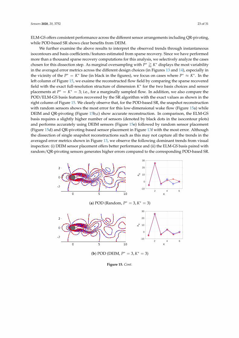
We further examine the above results to interpret the observed trends through instantaneousisocontours and basis coefficients/features estimated from sparse recovery. Since we have performedmore than a thousand sparse recovery computations for this analysis, we selectively analyze the caseschosen for this dissection step. As marginal oversampling with P∗ ' K∗ displays the most variabilityin the averaged error metrics across the different design choices (in Figures 13 and 14), especially inthe vicinity of the P∗ = K∗ line (in black in the figures), we focus on cases where P∗ ≈ K∗. In theleft column of Figure 15, we exaime the reconstructed flow field by comparing the sparse recoveredfield with the exact full-resolution structure of dimension K∗ for the two basis choices and sensorplacements at P∗ = K∗ = 3; i.e., for a marginally sampled flow. In addition, we also compare thePOD/ELM-GS basis features recovered by the SR algorithm with the exact values as shown in theright column of Figure 15. We clearly observe that, for the POD-based SR, the snapshot reconstructionwith random sensors shows the most error for this low-dimensional wake flow (Figure 15a) whileDEIM and QR-pivoting (Figure 15b,c) show accurate reconstruction. In comparison, the ELM-GSbasis requires a slightly higher number of sensors (denoted by black dots in the isocontour plots)and performs accurately using DEIM sensors (Figure 15e) followed by random sensor placement(Figure 15d) and QR-pivoting-based sensor placement in Figure 13f with the most error. Althoughthe dissection of single snapshot reconstructions such as this may not capture all the trends in theaveraged error metrics shown in Figure 13, we observe the following dominant trends from visualinspection: (i) DEIM sensor placement offers better performance and (ii) the ELM-GS basis paired withrandom/QR-pivoting sensors generates higher errors compared to the corresponding POD-based SR.

2 4 6K

-10

0

10

20

30

aK

(a) POD (Random, P∗ = 3, K∗ = 3)

2 4 6K

-10

0

10

20

30

aK

(b) POD (DEIM, P∗ = 3, K∗ = 3)

Figure 15. Cont.

Sensors 2020, 20, 3752 24 of 31

2 4 6K

-10

0

10

20

30

aK

(c) POD (QR, P∗ = 3, K∗ = 3)

5 10 15K

-10

0

10

20

30

aK

(d) ELM-GS (Random, P∗ = 3, K∗ = 3)

5 10 15K

-10

0

10

20

30a

K

(e) ELM-GS (DEIM, P∗ = 3, K∗ = 3)

5 10 15K

-10

0

10

20

30

aK

(f) ELM-GS (QR, P∗ = 3, K∗ = 3)

Figure 15. Left column: Comparison of line contours of streamwise velocity between the true flowfield (blue) and SR reconstruction (red) for Re = 100 using random and DEIM sensor placement atP∗ = 3, K∗ = 3 (marginally sampled) using both ELM-GS and POD SR. Right column: comparison ofthe estimated coefficients a using the entire data (blue circle) and the downsampled data (red star).

For the high-dimensional SST, we examine the instantaneous flow field and basis featuresestimated for the marginally oversampled case P∗ = 3 and K∗ = 2 in Figure 16. In particular, we notethat POD-based SR (Figure 16a–c) shows lower errors in the estimation of the basis features for DEIMwith a relative degradation in performance for both random and QR-pivoting-based sensors, increasingin that order. The ELM-GS counterpart in Figure 16d–f shows larger deviations from the ground truthfor random sensing while showing improved accuracy for DEIM and QR pivoting. Once again, thetrends from single snapshot reconstruction dissection of the NOAA-SST data are consistent with thosegleaned from the averaged error metrics in Figure 14; in particular, it is shown that ELM-GS performs

Sensors 2020, 20, 3752 25 of 31

better with QR-pivoting for this dataset as compared to POD-based SR. The superior performance ofDEIM for both these use cases is not surprising as the sensor placement algorithm directly leveragesknowledge of the basis vectors used in the SR step. However, the performance for both POD andELM-GS-based SR with QR-pivoting generates results that are problem-dependent. To investigate this,we inspect the matrix condition numbers below.

2 4 6 8 10 12 14 16 18K

500

0

500

1000

a K

(a) POD (Random, P∗ = 3, K∗ = 2)

2 4 6 8 10 12 14 16 18K

500

0

500

1000

a K

(b) POD (DEIM, P∗ = 3, K∗ = 2)

2 4 6 8 10 12 14 16 18K

0

500

1000

a K

(c) POD (QR, P∗ = 3, K∗ = 2)

5 10 15 20 25 30K

500

0

500

a K

(d) ELM-GS (Random, P∗ = 3, K∗ = 2)

Figure 16. Cont.

Sensors 2020, 20, 3752 26 of 31

5 10 15 20 25 30K

500

0

500

a K

(e) ELM-GS (DEIM, P∗ = 3, K∗ = 2)

5 10 15 20 25 30K

1000

500

0

500

a K

(f) ELM-GS (QR, P∗ = 3, K∗ = 2)

Figure 16. Left column: SR plot for sea surface temperature (SST) data with POD and ELM-GS basisusing random, DEIM and QR sensor placement sampled marginally (P∗ = 3, K∗ = 2). Right column:comparison of the estimated coefficients a using the entire data (blue circle) and the downsampleddata (red star). Contour color: dark blue represents a temperature equal to or below 15◦celsius and redrepresents a temperature equal or above 35◦celsius.

A key metric that impacts SR performance in linear estimation methods is the condition numberof the matrix, θ. Consistent with the least-squares minimization algorithm used in this work, weexplore the condition number for ΘTΘ in Table 2 for different bases, P∗ − K∗ combinations and sensorplacement methods for the reconstruction of the NOAA-SST dataset.

Table 2. Condition number estimation of ΘTΘ for both POD and ELM-GS basis-based SR usingdifferent sensor placement methods on sea surface temperature (SST) data. We have bolded the metricssmaller than a cutoff of 200 to highlight the low condition number cases.

Data: SST Random QR DEIM

POD

Marginally sampled(K* = 2, P* = 2) 2.95 × 105 1.21× 104 35.30

Marginally sampled(K* = 2, P* = 2 (+2)) 2.24× 103 1.28× 103 35.96

Marginally oversampled(K* = 2, P* = 3) 2.19× 102 1.22× 102 30.52

Oversampled(K* = 2, P* = 4) 66.98 36.84 23.64

ELM-GS

Marginally sampled(K* = 2, P* = 2) 5.87× 105 8.99× 103 1.72× 104

Marginally sampled(K* = 2, P* = 2 (+3)) 9.28× 103 1.22× 103 1.35× 103

Marginally oversampled(K* = 2, P* = 3) 197.18 74.78 74.42

Oversampled(K* = 2, P* = 4) 45.60 33.33 29.96

Sensors 2020, 20, 3752 27 of 31

We clearly see that POD-based SR shows smaller (O(100)) condition numbers for DEIM sensorplacement, even for the marginally sampled cases. For QR-pivoting and random sensing, we see thatsignificant oversampling with P∗ = 2K∗ is needed to ensure the condition number drops to reasonablevalues. In comparison, ELM-GS shows larger condition numbers than POD-based SR on average,but it is more sensitive to sensor budgets than sensor placement; that is, higher sensor budgets in themarginally oversampled and oversampled limits result in smaller condition numbers, even for randomand QR-pivoting-based sensing. This is in contrast to POD-based SR, which shows large conditionnumbers for similar SR designs. In summary, this analysis confirms that SR performance improveswith oversampling and sensor placement, which is tied to the data. While POD-based SR respondsbetter to high-quality data-informed sensor placement methods such as DEIM, ELM-GS respondsbetter to oversampling even with random and less-than-ideal sensing strategies. This explains thebetter SR accuracy generated for the NOAA-SST dataset using ELM-GS with QR-pivoting in themarginally sampled limit as compared to POD-based SR.

9. Discussion and Conclusions

In this work, we have presented a framework for data-driven sensor placement and sparsereconstruction using arbitrary non-orthogonal bases that may be encountered in a machine learningworkflow to handle complex dynamical systems. Although this work has adopted projections usingELM autoencoder maps for the low-dimensional representation of the data, the methods presentedhere can, in principle, be applied to any arbitrary class of basis vectors. Naturally, the success of theprocedure depends on the effectiveness of the basis vectors in approximating the space described by thedata. In addition to the lack of parsimony, arbitrary non-orthogonal basis tend to suffer from ineffectivesensor placement and high algorithmic complexity. In this study, we pair the ELM-basis, which suffersfrom these deficiencies, with a Gram–Schmidt orthogonalization step to build an ELM-GS basisspace as a mitigation step. We compare the basis structure, data-driven sensing and sparse recoveryperformance of ELM-GS with that using the POD basis.

We observe a reduction of nearly an order of magnitude in the basis dimension for ELM-GSto achieve desired data reconstruction accuracy, which in turn allows for a substantial reduction insensor requirements for sparse recovery. In fact, most linear estimation algorithms require a sensorbudget P & cK, where K is the desired recovery dimension and c is a pre-constant; that is, O(1− 10).The larger the K, the larger the sensor budget P. This relationship between P and K has been verifiedin our earlier work [48] and also confirmed in this study for the ELM-GS basis in Section 8.4. In fact,our analysis shows that the pre-constant c for the ELM-GS basis is ≈ 1.5. In addition, the topologyof the orthogonal ELM-GS modes mimics that of the POD modes for the same data. Therefore,the resulting data-driven sensor placements for both POD and ELM-GS bases show a significantoverlap of locations, as reported in Section 8.3. Further, the ELM-GS basis also possesses a built-inhierarchy similar to the POD basis—a trait useful in sparse recovery applications. This allows us toadopt computationally efficient least-squares minimization algorithms to solve the linear estimationproblem instead of a more expensive convex optimization problem in a l1 formulation.

Reconstructing low-dimensional flows from sparse data, we observe that both POD andELM-GS-based methods generate similar trends, with DEIM-based sensors showing the highestaccuracy followed by QR-pivoting and random sensing. On average, ELM-GS-based SR generatesslightly higher errors and slower error decay within the sensor budget P in a marginally oversampledregime for both classes of flows considered in the work. However, exceptions do exist, especiallywhen recovering high-dimensional systems such as the SST fields where the different linear estimationmethods show reduced accuracy. This is an expected consequence of dealing with multiscale systems,as most sparse estimation methods tend to do well in capturing the larger-scale dynamics but donot work as well at smaller scales. We note that POD-based SR responds better to improved sensorplacement from DEIM, while ELM-GS-based SR responds more to slight oversampling, even with

Sensors 2020, 20, 3752 28 of 31

less-than-ideal sensor placement, such as by using random sensors. This robustness of ELM-GS tosensor placement is valuable in practical settings where sensors are often distributed randomly.

Author Contributions: B.J. designed the study. S.M.A.A.M.; developed the codes with input from B.J.; S.M.A.A.M.carried out the analysis with input from B.J.; S.M.A.A.M. developed a partial draft of the manuscript; B.J. producedthe final written manuscript. All authors have read and agreed to the published version of the manuscript.

Funding: This research received no external funding.

Acknowledgments: We acknowledge computational resources from HPCC at Oklahoma State University.

Conflicts of Interest: The authors declare no conflict of interest.

References

1. Jayaraman, B.; Brasseur, J. Transition in Atmospheric Boundary Layer Turbulence Structure from Neutral toModerately Convective Stability States and Implications to Large-scale Rolls. arXiv 2018, arXiv:1807.03336

2. Jayaraman, B.; Brasseur, J. Transition in atmospheric turbulence structure from neutral to convective stabilitystates. In Proceedings of the 32nd ASME Wind Energy Symposium, National Harbor, MD, USA, 13–17January 2014; p. 0868.

3. Davoudi, B.; Taheri, E.; Duraisamy, K.; Jayaraman, B.; Kolmanovsky, I. Quad-rotor flight simulation inrealistic atmospheric conditions. AIAA J. 2020, 58, 1992–2004.

4. Allison, S.; Bai, H.; Jayaraman, B. Modeling trajectory performance of quadrotors under wind disturbances.In Proceedings of the 2018 AIAA Information Systems-AIAA Infotech@ Aerospace Meeting, Kissimmee, FL,USA, 8–12 January 2018; p. 1237.

5. Allison, S.; Bai, H.; Jayaraman, B. Wind estimation using quadcopter motion: A machine learning approach.Aerosp. Sci. Technol. 2020, 98, 105699.

6. Allison, S.; Bai, H.; Jayaraman, B. Estimating wind velocity with a neural network using quadcoptertrajectories. In Proceedings of the AIAA Scitech 2019 Forum, San Diego, CA, USA, 7–11 January 2019; p.1596.

7. Jayaraman, B.; Allison, S.; Bai, H. Estimation of Atmospheric Boundary Layer Turbulence Structure usingModelled Small UAS Dynamics within LES. In Proceedings of the AIAA Scitech 2019 Forum, San Diego,CA, USA, 7–11 January 2019; p. 1600.

8. Holmes P.; Lumley, J.L.; Berkooz, G.; Rowley, C.W. Turbulence, Coherent Structures, Dynamical Systems AndSymmetry; Cambridge University Press: New York, NY, USA, 2012.

9. Berkooz, G.; Holmes, P.; Lumley, J.L. The proper orthogonal decomposition in the analysis of turbulentflows. Annu. Rev. Fluid Mech. 1993, 25, 539–575.

10. Taira, K.; Brunton, S.L.; Dawson, S.T.; Rowley, C.W.; Colonius, T.; McKeon, B.J.; Schmidt, O.T.; Gordeyev, S.;Theofilis, V.; Ukeiley, L.S. Modal analysis of fluid flows: An overview. AIAA J. 2017, 4013–4041.

11. Jayaraman, B.; Lu, C.; Whitman, J.; Chowdhary, G. Sparse Convolution-based Markov Models for NonlinearFluid Flows. arXiv 2018, arXiv:1803.08222

12. Jayaraman, B.; Lu, C.; Whitman, J.; Chowdhary, G. Sparse feature map-based Markov models for nonlinearfluid flows. Comput. Fluids 2019, 191, 104252.

13. Rowley, C.W.; Dawson, S.T. Model reduction for flow analysis and control. Annu. Rev. Fluid Mech. 2017,49, 387–417.

14. Puligilla, S.C.; Jayaraman, B. Neural Networks as Globally Optimal Multilayer Convolution Architecturesfor Learning Fluid Flows. arXiv 2018, arXiv:1806.08234

15. Puligilla, S.C.; Jayaraman, B. Deep multilayer convolution frameworks for data-driven learning of fluidflow dynamics. In Proceedings of the 2018 Fluid Dynamics Conference, Atlanta, GA, USA, 25–29 June 2018;p. 3091.

16. Lu, C.; Jayaraman, B. Data-driven modeling for nonlinear fluid flows. In Proceedings of the 23rd AIAAComputational Fluid Dynamics Conference, Denver, CO, USA 5–9 June 2017; p. 3628.

17. Brunton, S.L.; Proctor, J.L.; Tu, J.H.; Kutz, J.N. Compressed sensing and dynamic mode decomposition.J. Comput. Dyn. 2015, 2, 165–191.

18. Bai, Z.; Wimalajeewa, T.; Berger, Z.; Wang, G.; Glauser, M.; Varshney, P.K. Low-dimensional approach forreconstruction of airfoil data via compressive sensing. AIAA J. 2014, 53, 920–933.

Sensors 2020, 20, 3752 29 of 31

19. Bright, I.; Lin, G.; Kutz, J.N. Compressive sensing based machine learning strategy for characterizing theflow around a cylinder with limited pressure measurements. Phys. Fluids 2013, 25, 127102.

20. Fukami, K.; Fukagata, K.; Taira, K. Super-resolution reconstruction of turbulent flows with machine learning.J. Fluid Mech. 2019, 870, 106–120.

21. Candès, E.J. Compressive sampling. In Proceedings of the International Congress of Mathematicians,Madrid, Spain, 22–30 August 2006; Volume 3, pp. 1433–1452.

22. Tropp, J.A.; Gilbert, A.C. Signal recovery from random measurements via orthogonal matching pursuit.IEEE Trans. Inf. Theory 2007, 53, 4655–4666.

23. Candès, E.J.; Wakin, M.B. An introduction to compressive sampling. IEEE Signal Process Mag. 2008, 25, 21–30.24. Needell, D.; Tropp, J.A. CoSaMP: Iterative signal recovery from incomplete and inaccurate samples.

Appl. Comput. Harmon. Anal. 2009, 26, 301–321.25. Bui-Thanh, T.; Damodaran, M.; Willcox, K. Aerodynamic data reconstruction and inverse design using

proper orthogonal decomposition. AIAA J. 2004, 42, 1505–1516.26. Willcox, K. Unsteady flow sensing and estimation via the gappy proper orthogonal decomposition.

Comput. Fluids 2006, 35, 208–226.27. Venturi, D.; Karniadakis, G.E. Gappy data and reconstruction procedures for flow past a cylinder.

J. Fluid Mech. 2004, 519, 315–336.28. Gunes, H.; Sirisup, S.; Karniadakis, G.E. Gappy data: To Krig or not to Krig? J. Comput. Phys. 2006,

212, 358–382.29. Gunes, H.; Rist, U. On the use of kriging for enhanced data reconstruction in a separated transitional

flat-plate boundary layer. Phys. Fluids 2008, 20, 104109.30. Everson, R.; Sirovich, L. Karhunen–Loeve procedure for gappy data. JOSA A 1995, 12, 1657–1664.31. Chaturantabut, S.; Sorensen, D.C. Nonlinear model reduction via discrete empirical interpolation. SIAM J.

Sci. Comput. 2010, 32, 2737–2764.32. Dimitriu, G.; Stefanescu, R.; Navon, I.M. Comparative numerical analysis using reduced-order modeling

strategies for nonlinear large-scale systems. J. Comput. Appl. Math. 2017, 310, 32–43.33. Zimmermann, R.; Willcox, K. An accelerated greedy missing point estimation procedure. SIAM J. Sci. Comput.

2016, 38, A2827–A2850.34. Saini, P.; Arndt, C.M.; Steinberg, A.M. Development and evaluation of gappy-POD as a data reconstruction

technique for noisy PIV measurements in gas turbine combustors. Exp. Fluids 2016, 57, 1–15.35. Schmid, P.J. Dynamic mode decomposition of numerical and experimental data. J. Fluid Mech. 2010,

656, 5–28.36. Hanagud, S.; de Noyer, M.B.; Luo, H.; Henderson, D.; Nagaraja, K. Tail buffet alleviation of high-performance

twin-tail aircraft using piezostack actuators. AIAA J. 2002, 40, 619–627.37. Cohen, K.; Siegel, S.; McLaughlin, T. Sensor placement based on proper orthogonal decomposition modeling

of a cylinder wake. In Proceedings of the 33rd AIAA Fluid Dynamics Conference and Exhibit, Orlando, FL,USA, 23–26 June 2003; p. 4259.

38. Barrault, M.; Maday, Y.; Nguyen, N.C.; Patera, A.T. An ‘empirical interpolation’method: application toefficient reduced-basis discretization of partial differential equations. C. R. Math. 2004, 339, 667–672.

39. Yildirim, B.; Chryssostomidis, C.; Karniadakis, G. Efficient sensor placement for ocean measurements usinglow-dimensional concepts. Ocean Model. 2009, 27, 160–173.

40. Manohar, K.; Brunton, B.W.; Kutz, J.N.; Brunton, S.L. Data-Driven Sparse Sensor Placement for Reconstruction:Demonstrating the Benefits of Exploiting Known Patterns. IEEE Control Syst. 2018, 38, 63–86.

41. Sarrate, R.; Nejjari, F.; Blesa, J. Sensor placement for monitoring. In Real-Time Monitoring and OperationalControl of Drinking-Water Systems; Springer: Glasgow, UK, 2017; pp. 153–173.

42. Cugueró-Escofet, M.À.; Puig, V.; Quevedo, J. Optimal pressure sensor placement and assessment for leaklocation using a relaxed isolation index: Application to the Barcelona water network. Control Eng. Pract.2017, 63, 1–12.

43. Sela, L.; Amin, S. Robust sensor placement for pipeline monitoring: Mixed integer and greedy optimization.Adv. Eng. Inform. 2018, 36, 55–63.

44. Huang, G.B.; Zhu, Q.Y.; Siew, C.K. Extreme learning machine: theory and applications. Neurocomputing2006, 70, 489–501.

Sensors 2020, 20, 3752 30 of 31

45. Huang, G.B.; Wang, D.H.; Lan, Y. Extreme learning machines: a survey. Int. J. Mach. Learn. Cybern. 2011,2, 107–122.

46. Zhou, H.; Huang, G.B.; Lin, Z.; Wang, H.; Soh, Y.C. Stacked extreme learning machines. IEEE Trans. Cybern.2015, 45, 2013–2025.

47. Al Mamun, S.; Lu, C.; Jayaraman, B. Extreme learning machines as encoders for sparse reconstruction. Fluids2018, 3, 88.

48. Jayaraman, B.; Al Mamun, S.; Lu, C. Interplay of Sensor Quantity, Placement and System Dimension inPOD-Based Sparse Reconstruction of Fluid Flows. Fluids 2019, 4, 109.

49. Tarantola, A. Inverse Problem Theory and Methods for Model Parameter Estimation; SIAM: Philadelphia, PA,USA, 2005; Volume 89

50. Arridge, S.R.; Schotland, J.C. Optical tomography: Forward and inverse problems. Inverse Prob. 2009,25, 123010.

51. Tarantola, A.; Valette, B. Generalized nonlinear inverse problems solved using the least squares criterion.Rev. Geophys. 1982, 20, 219–232.

52. Neelamani, R. Inverse problems in image processing. Ph.D. Thesis, Rice University, Houston, TX, USA, July 2004.53. Mallet, S. A Wavelet Tour of Signal Processing; Academic Press: San Diego, CA, USA, 1998.54. Donoho, D.L. Compressed sensing. IEEE Trans. Inf. Theory 2006, 52, 1289–1306.55. Baraniuk, R.G. Compressive sensing [lecture notes]. IEEE Signal Process Mag. 2007, 24, 118–121.56. Baraniuk, R.G.; Cevher, V.; Duarte, M.F.; Hegde, C. Model-based compressive sensing. IEEE Trans. Inf. Theory

2010, 56, 1982–2001.57. Sarvotham, S.; Baron, D.; Wakin, M.; Duarte, M.F.; Baraniuk, R.G. Distributed compressed sensing of jointly

sparse signals. In Proceedings of the Asilomar Conference on Signals, Systems, and Computers, PacificGrove, CA, USA, 1 November 2005; pp. 1537–1541.

58. Candès, E.J.; Romberg, J.; Tao, T. Robust uncertainty principles: Exact signal reconstruction from highlyincomplete frequency information. IEEE Trans. Inf. Theory 2006, 52, 489–509.

59. Candes, E.J.; Romberg, J.K.; Tao, T. Stable signal recovery from incomplete and inaccurate measurements.Commun. Pure Appl. Math. 2006, 59, 1207–1223.

60. Candes, E.J.; Tao, T. Near-optimal signal recovery from random projections: Universal encoding strategies?IEEE Trans. Inf. Theory 2006, 52, 5406–5425.

61. Candes, E.J.; Romberg, J.K. Signal recovery from random projections. In Computational Imaging III;International Society for Optics and Photonics, Electronic Imaging: San Jose, CA, USA, 2005; Volume 5674,pp. 76–87.

62. Chen, S.S.; Donoho, D.L.; Saunders, M.A. Atomic decomposition by basis pursuit. SIAM Rev. 2001,43, 129–159.

63. Tibshirani, R. Regression shrinkage and selection via the lasso. J. R. Stat. Soc. Ser. B (Methodol.) 1996, 267–288.64. Brunton, S.L.; Proctor, J.L.; Kutz, J.N. Discovering governing equations from data by sparse identification of

nonlinear dynamical systems. Proc. Natl. Acad. Sci. USA 2016, 113, 3932–3937.65. Sirovich, L. Turbulence and the dynamics of coherent structures. I. Coherent structures. Q. Appl. Math. 1987,

45, 561–571.66. Zhou, H.; Soh, Y.C.; Jiang, C.; Wu, X. Compressed representation learning for fluid field reconstruction from

sparse sensor observations. In Proceedings of the 2015 International Joint Conference on Neural Networks(IJCNN), Killarney, Ireland, 12–17 July 2015; pp. 1–6.

67. Kasun, L.L.C.; Zhou, H.; Huang, G.B.; Vong, C.M. Representational learning with extreme learning machinefor big data. IEEE Intell. Syst. 2013, 28, 31–34.

68. Candes, E.; Romberg, J. Sparsity and incoherence in compressive sampling. Inverse Prob. 2007, 23, 969.69. Csató, L.; Opper, M. Sparse on-line Gaussian processes. Neural Comput. 2002, 14, 641–668.70. Kubrusly, C.S.; Malebranche, H. Sensors and controllers location in distributed systems—A survey.

Automatica 1985, 21, 117–128.71. Chaturantabut, S.; Sorensen, D.C. A state space error estimate for POD-DEIM nonlinear model reduction.

SIAM J. Numer. Anal. 2012, 50, 46–63.

Sensors 2020, 20, 3752 31 of 31

72. Trefethen, L.N.; Bau, D., III. Numerical Linear Algebra; SIAM: Philadelphia, PA, USA, 1997; Volume 50.73. Cantwell, C.D.; Moxey, D.; Comerford, A.; Bolis, A.; Rocco, G.; Mengaldo, G.; De Grazia, D.; Yakovlev, S.;

Lombard, J.E.; Ekelschot, D.; others. Nektar++: An open-source spectral/hp element framework.Comput. Phys. Commun. 2015, 192, 205–219.

c© 2020 by the authors. Licensee MDPI, Basel, Switzerland. This article is an open accessarticle distributed under the terms and conditions of the Creative Commons Attribution(CC BY) license (http://creativecommons.org/licenses/by/4.0/).