bagwell 1 - verity software house · bagwell 7 the left panel shows a typical cell cycle analysis...

Modeling Kinetic Processes Without The Benefit Of Time As A Measurement

Bagwell 1

The literature is rich with articles describing mathematical models that can represent kineticprocesses. Many times, however, there are systems were it is difficult to directly measuretime or relative time. This lecture shows that even without the benefit of time as ameasurement, complex kinetic progressions can be successfully modeled. Theapplications of this technology were originally intended to study cellular progressions incytometry, but the theory is sufficiently general to handle any type of system where one canmake correlated measurements on numerous objects, but just can’t directly measure time.

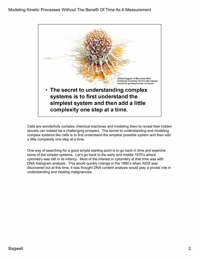
Cells are wonderfully complex chemical machines and modeling them to reveal their hiddensecrets can indeed be a challenging prospect. The secret to understanding and modelingcomplex systems like cells is to first understand the simplest possible system and then adda little complexity one step at a time.

One way of searching for a good simple starting point is to go back in time and examinesome of the simpler systems. Let’s go back to the early and middle 1970’s wherecytometry was still in its infancy. Most of the interest in cytometry at that time was withDNA histogram analysis. This would quickly change in the 1980’s when AIDS wasdiscovered but at this time, it was thought DNA content analysis would play a pivotal role inunderstanding and treating malignancies.


Bagwell 2

The first time I saw the story of “what is a DNA histogram” was in the mid-1970’s whenMack Fulwyler, the inventor of cell sorters, was giving a black-board talk on DNA histogramanalysis. From what we can gather, he was describing what he had been taught by MarvVan Dilla or Phil Dean at Los Alamos. He began by drawing two axis (1) which he labeledas Cell Age and DNA Content (2). Cell Age was a relative time scale that ranged from 0(right after division) to 1 (just before division). Cells begin the cycle with 2C (complements)of DNA and when the DNA synthetic machinery turns on, their nuclear DNA increases untilthe genome is duplicated at 4C (top graph). Thus, the cycle naturally divides into G1, S,and G2M phases along the Cell Age axis.

Mack then drew two more axes below the first graph. The x-axis was the same, Cell Age,but the y-axis was labeled as Number (Number of Events). He indicated that the density ofevents or cells immediately after cell division, Cell Age=0, for asynchronous population ofdividing cells was 2X and just before the cells divide, was X. For an exponentially growingpopulation the theoretical relationship was a decreasing exponential starting at 2X andending at X where X was dependent on the area under the curve.

He then drew two more axes with DNA Content on the x-axis and Number on the y-axisand labeled the graph as an Ideal DNA Histogram. He showed that the area under the G1part of the curve is represented as a spike with its height equal to the area and likewise, theG2M part of the curve was also a spike with the same height as its respective area. Hereasoned that as Cell Age moved from left to right, the DNA content would increase in theDNA Histogram plot and the number of events would decrease as a truncated exponential.


Bagwell 3

What Mack really did was show that the Ideal DNA Histogram could be derived from twofunctions that were related to Cell Age.


Bagwell 3

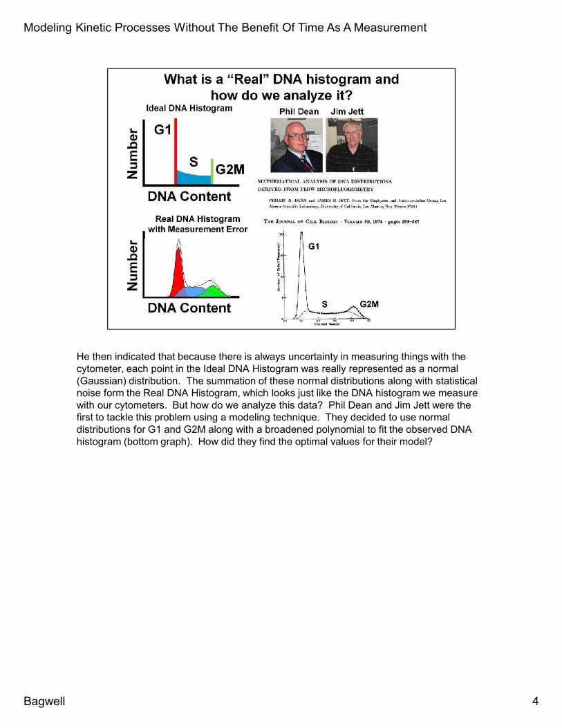
He then indicated that because there is always uncertainty in measuring things with thecytometer, each point in the Ideal DNA Histogram was really represented as a normal(Gaussian) distribution. The summation of these normal distributions along with statisticalnoise form the Real DNA Histogram, which looks just like the DNA histogram we measurewith our cytometers. But how do we analyze this data? Phil Dean and Jim Jett were thefirst to tackle this problem using a modeling technique. They decided to use normaldistributions for G1 and G2M along with a broadened polynomial to fit the observed DNAhistogram (bottom graph). How did they find the optimal values for their model?


Bagwell 4

The modeling process involves mathematically quantifying the overall degree of differencebetween the model and the observed data points. Typically, this is done by summing theweighted squared differences known as chi-square. For a single parameter in the model,this can be visualized as a special response function that has some set of valleys, whereone is deeper than all the others. This valley is called the true minimum. Modeling beginswith an estimate that is close enough to the True Minimum that it can follow the gradientthrough an iterative process to the optimum value. This method is easily extended to manymodel parameters. It’s important to distinguish between a model parameters and acytometric measurement often called a parameter.

The Dean and Jett broadened polynomial required the optimization of 9 model parameters.It began a vigorous search for the optimal model for DNA histogram analysis.


Bagwell 5

Quite a few DNA models have been proposed over the years and some of them are shownabove. Sometime in the middle 1990’s the estimation and modeling algorithms reached alevel of sophistication where the modeling process became largely automatic no matterwhat the complexity of the DNA sample. The program MutliCycle evolved from principallyPeter Rabinovitches work and ModFit resulted from mine.


Bagwell 6


Bagwell 7

The left panel shows a typical cell cycle analysis with one of the testing data sets and theright panel shows conventional gating analysis of the same data. Cell cycle analyses arenow completely automatic and therefore the results from the program are reproducible.Any operator given the same data should receive the same exact results.


Bagwell 8

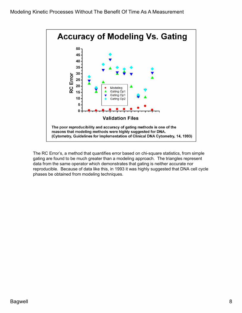
The RC Error’s, a method that quantifies error based on chi-square statistics, from simplegating are found to be much greater than a modeling approach. The triangles representdata from the same operator which demonstrates that gating is neither accurate norreproducible. Because of data like this, in 1993 it was highly suggested that DNA cell cyclephases be obtained from modeling techniques.

Unfortunately, is was very difficult to extend this modeling approach to multiple dimensions.The desire was to be able to model immunofluorescence data, but the complexity of thedata and the resultant models was large enough to make computer solutions impractical.Although most cytometrists knew that gating was subjective and error prone, it was largelyignored because there was no viable alternative.


Bagwell 9

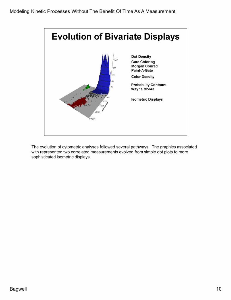
The evolution of cytometric analyses followed several pathways. The graphics associatedwith represented two correlated measurements evolved from simple dot plots to moresophisticated isometric displays.


Bagwell 10

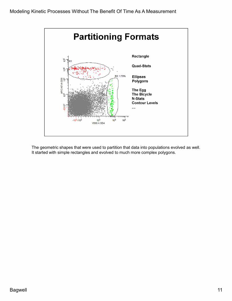
The geometric shapes that were used to partition that data into populations evolved as well.It started with simple rectangles and evolved to much more complex polygons.


Bagwell 11

Initially we used simple gates where a histogram was gated on events that were inside arectangle. Fairly early on, this process was abstracted in the Ortho 2150 computer systemand refined by Ray Lafebvre in his development of LYSYS. Over time it was found thatmost immunologists wanted to divide their populations into ever smaller populations usinghierarchical or containment gates. This work was pioneered by Wayne Moore and MarioRoederer.


Bagwell 12

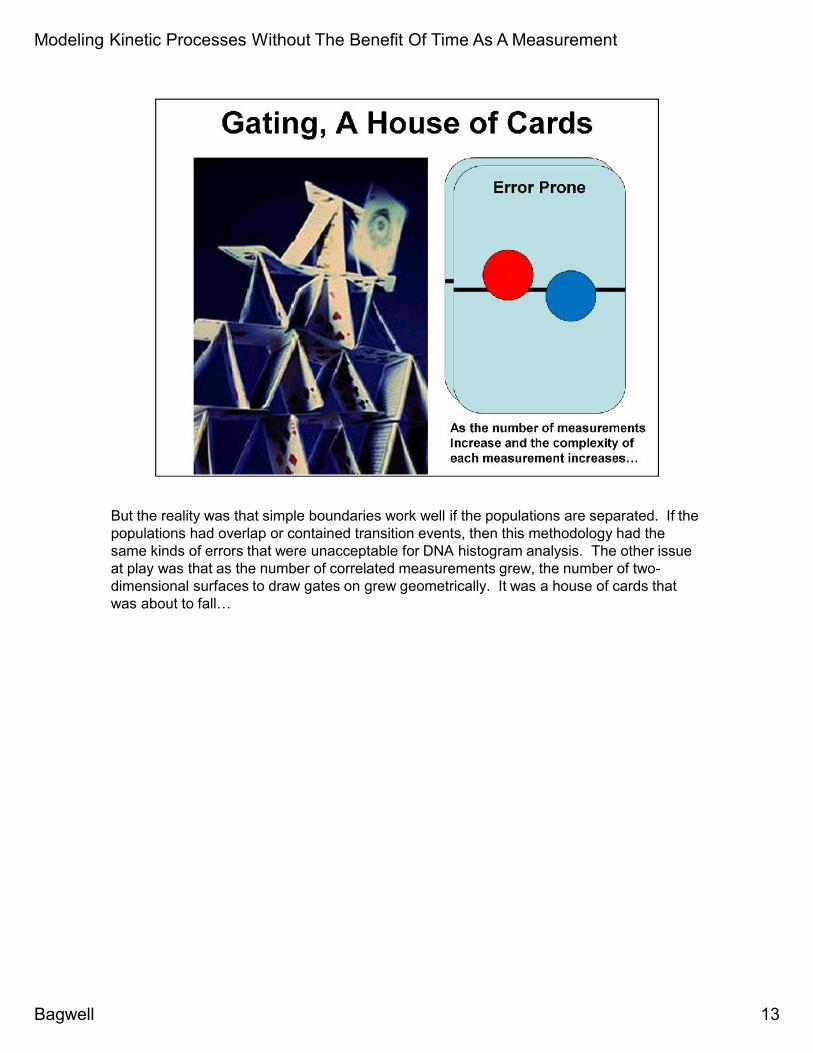
But the reality was that simple boundaries work well if the populations are separated. If thepopulations had overlap or contained transition events, then this methodology had thesame kinds of errors that were unacceptable for DNA histogram analysis. The other issueat play was that as the number of correlated measurements grew, the number of two-dimensional surfaces to draw gates on grew geometrically. It was a house of cards thatwas about to fall…


Bagwell 13

Knowing what we now know about modeling complex systems, it would be wonderful to goback in time and change how we initially viewed the modeling process as it pertained tocytometric DNA histograms. We were a lot closer to the correct solution than most peoplerealize.


Bagwell 14

If we could go back in time, I would come up to Mack after he gave his talk on what a DNAhistogram is in and talk with him. I would say something like, Mack, I enjoyed your talk, butI think I can show you a much better way of understanding and analyzing DNA histograms.Mack might say something like, “OK, let’s hear it.”

First of all, Mack, if you eliminate Cell Age and do the modeling in measurement space,modeling will essentially be relegated to the one-dimensional world of DNA histogramanalysis for over 30 years. So, let’s begin by not eliminating Cell Age and get rid of thisconcept of the Ideal DNA Histogram. This path doesn’t lead us to where we need to go.


Bagwell 15

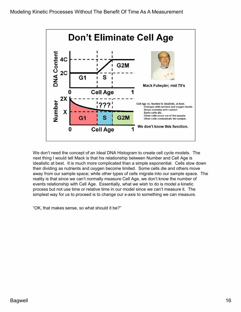
We don’t need the concept of an Ideal DNA Histogram to create cell cycle models. Thenext thing I would tell Mack is that his relationship between Number and Cell Age isidealistic at best. It is much more complicated than a simple exponential. Cells slow downtheir dividing as nutrients and oxygen become limited. Some cells die and others moveaway from our sample space; while other types of cells migrate into our sample space. Thereality is that since we can’t normally measure Cell Age, we don’t know the number ofevents relationship with Cell Age. Essentially, what we wish to do is model a kineticprocess but not use time or relative time in our model since we can’t measure it. Thesimplest way for us to proceed is to change our x-axis to something we can measure.

“OK, that makes sense, so what should it be?”


Bagwell 16

What we can do is define the Number relationship such that it has constant cell density allthe way along the x-axis (see above). Since our boundaries are 0 to 1, this means that they-axis intercept is simply the number of events measured or n.

Mack puts his hand on his chin and says, “well, if you are going to make that definition, thenthe boundaries between G1 and S and S and G2M will need to change.”

That’s right, Mack, let’s change these boundaries to where ever they need to go to beconsistent with our data (arrows).


Bagwell 17

Notice, Mack, that these boundaries are now at the fraction of G1 (fG1) and the fraction ofG1 plus the fraction of S (fG1+fS). In other words, as soon as we defined the constantdensity relationship, our x-axis changed to cumulative fraction. Just to make this conceptclearer, let’s use a specific example. If the fraction of G1 in our population were 0.6, thenthe first G1/S boundary would be placed at 0.6. If the S-phase had a fraction of 0.15, thenthe second S/G2M boundary would be at 0.6+0.15 or 0.75.

“OK, I see that”, Mack says. “But that means that our DNA Content vs. CumulativeFraction function needs to be changed as well for the model to be totally consistent.”

That’s right, Mack, let’s make that change as well.


Bagwell 18

At this point, Mack, we have a consistent model of cell cycle involving two relationships withCumulative Fraction.

“OK, Bruce, I’m liking this so far. What’s next?”

The next enhancement to your DNA histogram story involves how you introduced thevariability of the measurement and biology into the model. The correct way of doing it,Mack, is to integrate that information into this model at this level. We can do this byproviding our model with 95% confidence limits. In the case of DNA content measured withlinear amplifiers, this means that the width of our 95% confidence limits will increase asDNA content increases.

“Bruce, I can see that this model now captures all the essential information that is containedin a DNA histogram, but what is troubling me is how are you going to fit it to the observeddata?”

Mack, there are a few more steps we need to take before we’re ready to do this.


Bagwell 19

The first step is that we can merge the DNA Content and Number axes together by creatinga probability distribution from both of them. If we were to look at this function using coloredcontours, it would look as shown above. This one plot merges cumulative fraction orprogression (x-axis), DNA Content (y-axis), and probability (z-axis).

Before examining how to analyze the data, it’s easier to first see how this data structure cangenerate DNA histogram-like data. Models should be able to generate as well as analyzedata. The procedure is quite simple. First, we randomly choose a location along theprogression axis (1). Given this location, we use the probability distribution at this locationto randomly pick our DNA Content (2). This means that we are using the probabilityinformation in the vertical direction to appropriately choose the DNA Content value. If werepeat this procedure thousands of times, we produce a set of data that is very much likethe data we obtain when we measure cells for their DNA content.


Bagwell 20

“OK, Bruce, I think I can visualize the synthesis process, but I’m still troubled by how all thisallows us to fit our model to an observed DNA histogram? “

It turns out, Mack, that if you reverse this random picking process, you set the stage foranalysis. By reversing, I mean that when you observe a single DNA content value (y-axis),you use the above probability distribution to randomly pick a horizontal position (1) alongthe progression axis. Usually we bin this axis into a set of 100 states. If you repeat thisprocess thousands of times, you will obtain a uniform distribution of state frequencies if themodel is consistent with the observed data. This is not an approximation, Mack. If themodel and the data are consistent with each other, the resultant state frequencies will be asuniform as possible given counting error.

We can quantify how uniform this distribution is use this as a model response function tosearch for the best model parameters. That’s how the system can fit observed data to ournew model. We call this approach Probability State Modeling or PSM.


Bagwell 21

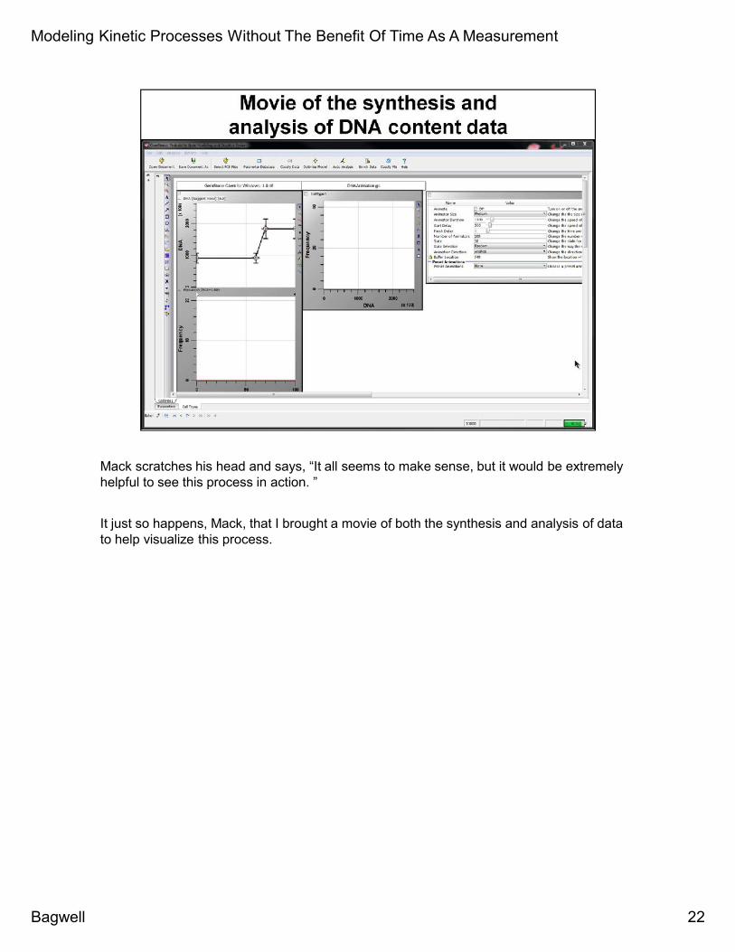
Mack scratches his head and says, “It all seems to make sense, but it would be extremelyhelpful to see this process in action. ”

It just so happens, Mack, that I brought a movie of both the synthesis and analysis of datato help visualize this process.


Bagwell 22


Bagwell 23


Bagwell 24

“I see how this works now, Bruce. Just as a point of curiosity, how accurate is it inestimating %G1, %S, and %G2M as compared to the more traditional modeling methods?”

If we compare the computed errors using chi-square statistics for Probability State Modeling(PSM) and Cell Cycle Analysis (CCA), we find that in general both methods produceanalysis results that are quite comparable. PSM does have a few advantages over CCA,however. With traditional modeling, if you have two model components of similar shapethat are overlapped, CCA will become unstable and yield unreliable results; whereas, PSMsimply assigns each model component equal numbers of events and is perfectly stable.

“I assume, Bruce, that you’re showing me this new approach because it does somethingthat traditional modeling methods can not.”

That’s right, Mack. We are now in a position to model data with numerous correlatedmeasurements. By defining our model as we have, we can potentially model any numberof markers that modulate over some progression. This is something we were never able todo before.

We can theoretically add any number of markers we want to our model of progression. Thefirst marker could be DNA, but it could be any other relation as well. It’s also very easy toextend the algorithms to either synthesize data from all these parameter profiles or toanalyze them.


Bagwell 25


Bagwell 26

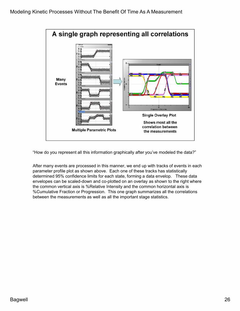
“How do you represent all this information graphically after you’ve modeled the data?”

After many events are processed in this manner, we end up with tracks of events in eachparameter profile plot as shown above. Each one of these tracks has statisticallydetermined 95% confidence limits for each state, forming a data envelop. These dataenvelopes can be scaled-down and co-plotted on an overlay as shown to the right wherethe common vertical axis is %Relative Intensity and the common horizontal axis is%Cumulative Fraction or Progression. This one graph summarizes all the correlationsbetween the measurements as well as all the important stage statistics.

“Just a few more questions, Bruce. It seems to me that it should be very complicated tofigure out the proper parameter profile to use for each measurement. For DNA, it was easysince this is a well-known relationship to most biologists. But some of the new markers arenot so well-known. How do you handle this complexity issue?”

It ends up that it is far easier to model these complex populations than you might think.Mack, the way to get at this answer is to use a hypothetical example and see how to applythe technique of probability state modeling to it. Let’s say we have some five-color datathat looks at five markers (A, B, C, D, and E) for two hypothetical populations. To getstarted we need to know that the population of interest for us has a lot of C marker on itssurface (C+). We refer to this as our selection marker. To tell the system we’re interestedin C+ we use a constant parameter profile that selects for the events of interest (1).

We then choose a relation that we do know something about. In this case, suppose weknow that Marker A is up-regulated in our progression much like our DNA content exampleand we model it as we did our DNA (2).


Bagwell 27

What happens next is really quite amazing. Once the system has modeled Marker A, it haspartially ordered the events along the x-axis. This means that when we look at Marker B,we can usually tell how it varies with A without any a priori knowledge. The decision of howto model Marker B can be entirely automatic (3).

After it has finished with B, it now can use both the A and B information to better define D.An appropriate parameter profile can then be chosen for D completely automatically. Thisprocess continues until all the markers have been modeled.

“You don’t have a movie that shows this process in action do you? “

Of course I do…


Bagwell 28


Bagwell 29

“OK, Bruce, let’s see some actual applications with some of the instruments capable oftaking numerous correlated measurements.”

The first application we applied this technique to was modeling the B-cell lineage in humanbone marrow. When examining normal B-cell lineage progression, it is quite impressive tosee the sharp transitions that B-cells go through in the bone marrow. When thedimensionality issue is eliminated, it is easier to appreciate the genetic program at work.


Bagwell 30

Another application is the changes in CD8 T-cells as they interact with specific antigens inthe peripheral blood.


Bagwell 31

This slide shows a PNH abstract and poster shown at CYTO 2011 by Ben Hunsberger,demonstrating how PSM can automate this widely ordered test. Interestingly, these modelshave no progressions at all.


Bagwell 32

Stem cell enumeration, CYTO2011 abstract and poster by Don Herbert, is another exampleof the PSM automation capabilities where the models have no progressions.


Bagwell 33

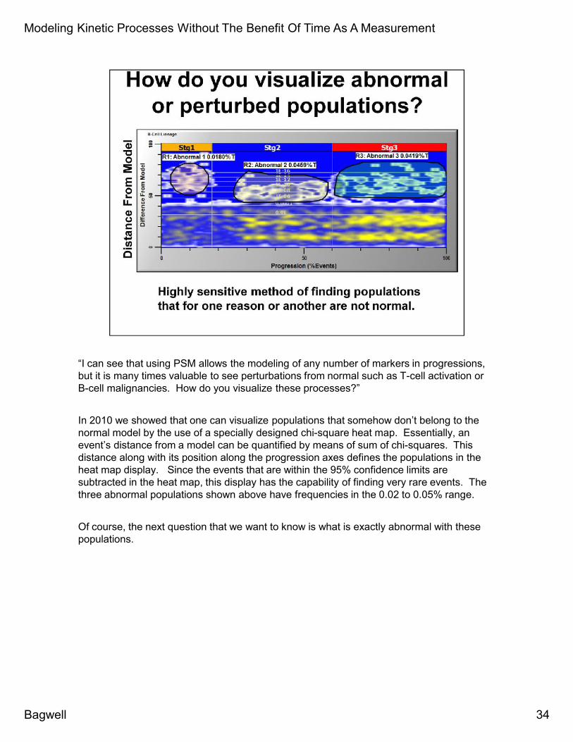
“I can see that using PSM allows the modeling of any number of markers in progressions,but it is many times valuable to see perturbations from normal such as T-cell activation orB-cell malignancies. How do you visualize these processes?”

In 2010 we showed that one can visualize populations that somehow don’t belong to thenormal model by the use of a specially designed chi-square heat map. Essentially, anevent’s distance from a model can be quantified by means of sum of chi-squares. Thisdistance along with its position along the progression axes defines the populations in theheat map display. Since the events that are within the 95% confidence limits aresubtracted in the heat map, this display has the capability of finding very rare events. Thethree abnormal populations shown above have frequencies in the 0.02 to 0.05% range.

Of course, the next question that we want to know is what is exactly abnormal with thesepopulations.


Bagwell 34

The first comprehensive method of finding all phenotype combinations was the PRISMboard designed by Jim Wood and the EPICS Division team. Later, in the 1990’s, this typeof logic was generalized to include the results of boolean gates with WinList’s FCOM logic.More recently, Mario Roederer has used the same kind of logic and generalized it toinclude patient group averaging and the use of pie charts to graphically represent all thephenotypes.

Modeling of progressions offers the opportunity to extend the concept gates (in or out) tothree states (normal, lower-than-normal, and higher-than-normal). Also, these calculationscan be applied within specific stages of the progressions referred to as zones (see aboveslide, bottom). Probably most important, however, is that since it is a result of modeling, allboundaries are positioned automatically with no human bias.


Bagwell 35

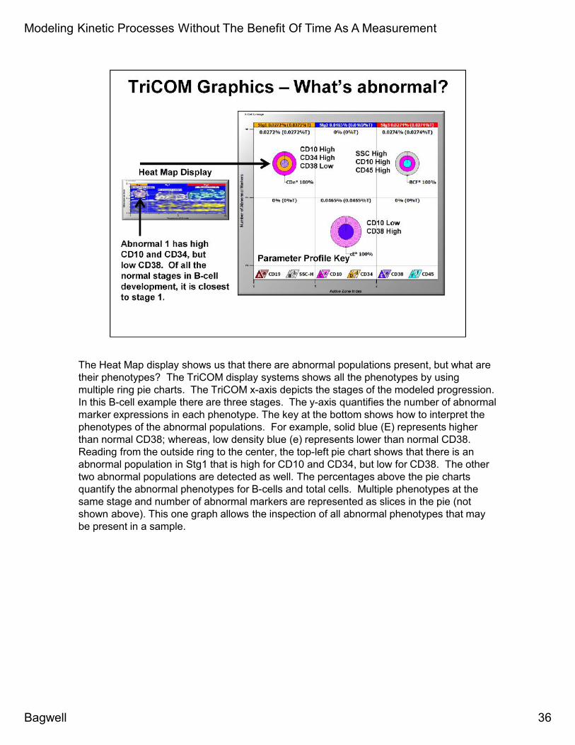
The Heat Map display shows us that there are abnormal populations present, but what aretheir phenotypes? The TriCOM display systems shows all the phenotypes by usingmultiple ring pie charts. The TriCOM x-axis depicts the stages of the modeled progression.In this B-cell example there are three stages. The y-axis quantifies the number of abnormalmarker expressions in each phenotype. The key at the bottom shows how to interpret thephenotypes of the abnormal populations. For example, solid blue (E) represents higherthan normal CD38; whereas, low density blue (e) represents lower than normal CD38.Reading from the outside ring to the center, the top-left pie chart shows that there is anabnormal population in Stg1 that is high for CD10 and CD34, but low for CD38. The othertwo abnormal populations are detected as well. The percentages above the pie chartsquantify the abnormal phenotypes for B-cells and total cells. Multiple phenotypes at thesame stage and number of abnormal markers are represented as slices in the pie (notshown above). This one graph allows the inspection of all abnormal phenotypes that maybe present in a sample.


Bagwell 36


Bagwell 37

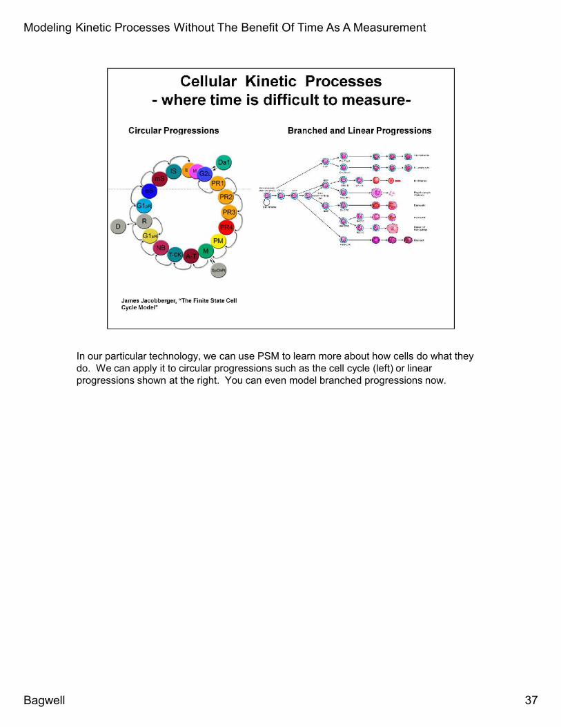
In our particular technology, we can use PSM to learn more about how cells do what theydo. We can apply it to circular progressions such as the cell cycle (left) or linearprogressions shown at the right. You can even model branched progressions now.

Any time it is difficult or impossible to measure time and you want to model the kineticprocess, probability state modeling can be used. It works best when there are manymeasured objects with correlated measurements.


Bagwell 38

I should make a few comments about clustering before leaving this lecture. Clustering hasalways shown great promise since it scales very well with number of correlatedmeasurements. Initially Gary Salzman and Robert Murphy explored its potential incytometry starting late in the 1960’s and published a number of papers and chaptersthrough out the 1970’s and 1980’s. Since then, there have been numerous differentstrategies proposed for clustering, but it really has never become mainstream. I suspectthe reason for this is three-fold. The first issue is that clustering algorithms many timesdivide well-known populations into multiple parts and also many times fails to find low-frequency continuums that connect the clusters. The second issue is that clusteringgenerally has a number of user-defined parameters that can radically change the finalsolution. The animation shows an example of how the boundaries around clusters cansuddenly and dramatically change. The third issue is more insidious. After the clusteringalgorithm has identified the clusters, the next question is do these cluster represent. Sincemost clustering algorithms are devoid of biologic information, the user or biologist must usetraditional methods to identify the found clusters. If clustering is suppose to be a solution tothe dimensionality problem, requiring the inspection of bivariates to understand themeaning of the clusters is not really a solution that will work for very high-dimensional data.

Recently, a new clustering method has been devised by Sean Bendall at Stanford that mayobviate some of these limitations. Since it creates numerous micro-clusters via a processcalled agglomeration, it may not have a tendency to eliminate the continuums betweenpopulations that we normally use to understand the meaning of the data. Also, it looks asthough it has some biologic constraints so that the cluster interrelationships areimmediately evident by someone with some knowledge of the biologic process being


Bagwell 39

studied. However, it is new and it is not yet known how sensitive it is to subjective userdecisions and how automated it can become over the next few years.


Bagwell 39


Bagwell 40


Bagwell 41

The Verity team made the creation of Probability State Modeling possible. Thanks guys!


Bagwell 42

bagwell 1 - verity software house · bagwell 7 the left panel shows a typical cell cycle analysis...

Documents