backbone fragility and the local search cost peak

Journal of Artificial Intelligence Research 12 (2000) 235-270 Submitted 12/99; published 5/00

Backbone Fragility and the Local Search Cost Peak

Josh Singer [email protected]

Division of Informatics, University of Edinburgh80 South Bridge, Edinburgh EH1 1HN, United Kingdom

Ian P. Gent [email protected]

School of Computer Science, University of St. AndrewsNorth Haugh, St. Andrews, Fife KY16 9SS, United Kingdom

Alan Smaill [email protected]

Division of Informatics, University of Edinburgh80 South Bridge, Edinburgh EH1 1HN, United Kingdom

Abstract

The local search algorithm WSat is one of the most successful algorithms for solvingthe satisfiability (SAT) problem. It is notably effective at solving hard Random 3-SATinstances near the so-called ‘satisfiability threshold’, but still shows a peak in search costnear the threshold and large variations in cost over different instances. We make a numberof significant contributions to the analysis of WSat on high-cost random instances, usingthe recently-introduced concept of the backbone of a SAT instance. The backbone is the setof literals which are entailed by an instance. We find that the number of solutions predictsthe cost well for small-backbone instances but is much less relevant for the large-backboneinstances which appear near the threshold and dominate in the overconstrained region.We show a very strong correlation between search cost and the Hamming distance to thenearest solution early in WSat’s search. This pattern leads us to introduce a measure of thebackbone fragility of an instance, which indicates how persistent the backbone is as clausesare removed. We propose that high-cost random instances for local search are those withvery large backbones which are also backbone-fragile. We suggest that the decay in costbeyond the satisfiability threshold is due to increasing backbone robustness (the oppositeof backbone fragility). Our hypothesis makes three correct predictions. First, that thebackbone robustness of an instance is negatively correlated with the local search cost whenother factors are controlled for. Second, that backbone-minimal instances (which are 3-SATinstances altered so as to be more backbone-fragile) are unusually hard for WSat. Third,that the clauses most often unsatisfied during search are those whose deletion has the mosteffect on the backbone. In understanding the pathologies of local search methods, we hopeto contribute to the development of new and better techniques.

1. Introduction

Why do some problem instances require such a high computational cost for algorithms tosolve? Answering this question will help us to understand the interaction between searchalgorithms and problem instance structure and can potentially suggest principled improve-ments, for example the Minimise-Kappa heuristic (Gent, MacIntyre, Prosser, & Walsh,1996; Walsh, 1998).

In this paper we study the propositional satisfiability problem (SAT). SAT is importantas it was the first and is perhaps the archetypal NP-complete problem. Furthermore, many

c©2000 AI Access Foundation and Morgan Kaufmann Publishers. All rights reserved.

Singer, Gent & Smaill

AI tasks of practical interest such as constraint satisfaction, planning and timetabling canbe naturally encoded as SAT instances.

A SAT instance C is a propositional formula in conjunctive normal form. C is a bagof m clauses which represents their conjunction. A clause is a disjunction of literals, whichare Boolean variables or their negations. The variables constitute a set of n symbols V . Anassignment is a mapping from V to {true, false}. The decision question for SAT asks whetherthere exists an assignment which makes C true under the standard logical interpretationof the connectives. Such an assignment is a solution of the instance. If there is a solution,the SAT instance is said to be satisfiable. In this study, assignments where a few clausesare unsatisfied are also important. We refer to these as quasi-solutions. k-SAT is the SATproblem restricted to clauses containing k literals. Notably, the k-SAT decision problemis NP-hard for k ≥ 3 (Cook, 1971). In several NP-hard decision problems, such as 3-SAT, certain probabilistic distributions of instances parameterised by a “control parameter”exhibit a sharp threshold or “phase transition” in the probability of there being a solution(Cheeseman, Kanefsky, & Taylor, 1991; Gent et al., 1996; Mitchell, Selman, & Levesque,1992). There is a critical value of the control parameter such that instances generatedwith the parameter in the region lower than the critical value (the underconstrained region)almost always have solutions. Those generated from the overconstrained region where thecontrol parameter is higher than the critical value almost always have no solutions.

In many problem distributions, this threshold is associated with a peak in search costfor a wide range of algorithms. Instances generated from the distribution with the controlparameter near the critical value are hardest and cost decays as we move from this valueto lower or higher values. This behaviour is of interest to basic AI research. Being devoidof any regularities, random instances represent the challenge faced by an algorithm in theabsence of any assumptions about the problem domain, or once all knowledge about it hasbeen exploited in the design of the algorithm or transformation of the problem instance.

Random k-SAT is a parameterised distribution of k-SAT instances. In Random k-SAT,n is fixed and the control parameter is m/n. Varying m/n produces a sharp threshold in theprobability of satisfiability and an associated cost peak for a range of complete algorithms(Crawford & Auton, 1996; Larrabee & Tsuji, 1992). The cost peak pattern in Randomk-SAT has been conjectured to extend to all reasonable complete methods by Cook andMitchell, (1997) who also give an overview of analytic and experimental results on theaverage-case hardness of SAT distributions.

In this paper we study the behaviour of local search on Random k-SAT. The term localsearch encompasses a class of procedures in which a series of assignments are examined withthe objective of finding a solution. The first assignment is typically selected at random.Local search then proceeds by moving from one assignment to another by “flipping” (i.e.inverting) the truth value of a single variable. The variable to flip is chosen using a heuristicwhich may include randomness, an element of hill-climbing (for example on the number ofsatisfied clauses) and memory. Usually, local search is incomplete for the SAT decisionproblem: there is no guarantee that if a solution exists, it will be found within any timebound. Unlike complete procedures, local search cannot usually prove for certain that nosolution exists.

It is a relatively recent discovery (e.g. Selman, Levesque and Mitchell, 1992) that theaverage cost for local search procedures scales much better than that of the best complete

236


procedures at the critical value of m/n in Random 3-SAT. More recent studies, (e.g. Parkesand Walser, 1996) have confirmed this in detail. Therefore in any system where completenessmay be sacrificed, local search procedures have an important role to play, and this is whythey have generated so much interest in recent years.

If we restrict ourselves to those instances of the distribution which are satisfiable andincrease the control parameter, there is a peak in the cost for local search procedures tosolve the instances near the critical value in several constraint-like problems (Clark, Frank,Gent, MacIntyre, Tomov, & Walsh, 1996; Hogg & Williams, 1994). In the underconstrainedregion, the average cost increases with m/n due to the decreasing number of solutions perinstance (Clark et al., 1996). However, in the overconstrained region, the cost decreases withm/n although the number of solutions per instance continues to fall. Several researchershave noted this fact with surprise (Clark et al., 1996; Parkes, 1997; Yokoo, 1997) since thenumber of solutions does not change in any special way near the critical value. Why, then,should the cost of satisfiable instances peak near the critical value, and then decay?

Parkes (1997) provided an appealing answer to the first part of this question in his studyof the backbone of satisfiable Random 3-SAT instances. For satisfiable SAT instances, thebackbone is the set of literals which are logically entailed by the clauses of the instance1.Variables which appear in these entailed literals are each forced to take a particular truthvalue in all solutions. Parkes’ study demonstrated that in instances from the undercon-strained region, only a small fraction of the variables, if any, appear in the backbone.However, as the control parameter is increased towards the critical value, a subclass ofinstances which have large backbones, mentioning around 75-95% of the variables, rapidlyemerges. Soon after the control parameter is increased into the overconstrained region theselarge-backbone instances account for all but a few of the satisfiable instances. Parkes alsoshowed that for a fixed value of the control parameter, the cost for the local search proced-ure WSat is strongly influenced by the size of the backbone. This suggests that the peak inaverage WSat cost near the critical value as the control parameter is increased may be dueto the emergence of large-backbone instances at this point. Parkes noted that for any givensize of backbone, the cost is actually higher for instances from the underconstrained regionand falls as the control parameter is increased. He also identified this fall as indicative ofanother factor which produces the overall peak in cost. The main aim of this paper is toidentify the factor responsible for this pattern; why are some instances with a certain sizeof backbone more costly to solve than others?

The remainder of the paper is organised as follows. In Section 2 we review the detailsof the WSat algorithm and the Random k-SAT distribution and discuss the experimentalconditions which were used. We also elucidate the patterns in cost which we intend toexplain and show how the number of solutions and the backbone size interact. In Section3 we identify a remarkable pattern in WSat’s search behaviour which clearly distinguisheshigh cost from lower cost instances of a certain backbone size. WSat is usually drawnearly on in the search to quasi-solutions where a few clauses are unsatisfied. On high costinstances, these quasi-solutions are distant from the nearest solution, while on lower costinstances of equal backbone size, they are less distant. In Section 4 we develop a causalhypothesis, postulating a structural property of instances which induces a search space

1. Here, our use of the term “backbone” follows Monasson, Zecchina, Kirkpatrick, Selman and Troyansky(1999a, 1999b) whose definition of the backbone is equivalent to ours for satisfiable instances.

237


structure which in turn causes the observed search behaviour and thus the cost pattern. Wesuggest that instances of a certain backbone size are of high cost when they are backbone-fragile, i.e. when the removal of a few clauses at random results in an instance with agreatly reduced backbone size. We discuss how this property may be measured and showhow as the control parameter is increased, instances of a certain backbone size become lessbackbone-fragile.

A hypothesis is only of true scientific merit if it makes correct predictions. Our hy-pothesis made three correct predictions for which we provide experimental evidence. InSection 5 we show that the degree to which an instance is backbone-fragile accounts forsome of the variance in cost when the control parameter and the backbone-size are fixed.In Section 6 we consider the generation of instances which are very backbone-fragile. Ifclauses are removed such that the backbone is unaffected, we found that the resulting in-stances became progressively more backbone-fragile. Eventually, no more clauses can beremoved without affecting the backbone and the instance is said to be backbone minimal.Our hypothesis correctly predicts that as clauses are removed in this way from Random3-SAT instances, the cost becomes considerably higher. In Section 7 we show that the hy-pothesis makes a correct prediction relating to the search behaviour: the clauses which aremost often unsatisfied during search are those whose removal most affects the backbone. InSection 8 we relate this study to previous research and give suggestions for further work.Finally, Section 9 concludes.

2. Background

In this section we discuss the local search algorithm WSat, the measurement of computa-tional cost for it and its representativeness of local search algorithms in general. We alsoreview the Random k-SAT distribution and the overall cost pattern for WSat on Randomk-SAT. Finally we look at how backbone size and the number of solutions interact to affectthe cost.

2.1 The WSat Algorithm

The term WSat was first introduced by Selman et al. (1994). It refers to a local searcharchitecture which has also been the subject of a number of subsequent empirical studies(Hoos, 1999a; McAllester, Selman, & Kautz, 1997; Parkes & Walser, 1996; Parkes, 1997).A pseudocode outline of the WSat algorithm is given in Figure 1. An important featureof WSat is that, unlike earlier local search algorithms, it chooses an unsatisfied clauseand then flips a variable appearing in that clause: Select-variable-from-clause mustreturn a variable mentioned in clause. This architecture was first seen in the “random walkalgorithm” due to Papadimitriou (1991). WSat may use different strategies for Select-

variable-from-clause. In this study, we used the “SKC” strategy introduced by Selman,Kautz and Cohen (1994); we refer to this combination simply as WSat. Pseudocode forthe SKC strategy is given in Figure 2.

We follow Hoos (1998) in our approach to measuring the computational cost of SATinstances for our local search algorithm WSat. Rather than run-times, we measure run-lengths : the number of flips taken to find a solution. We set the noise level p to 0.55, whichHoos found to be approximately optimal on Random 3-SAT. Hoos and Stutzle (1998) showed

238


WSat(C, Max-tries, Max-flips, p)for i = 1 to Max-tries

T := a random assignmentfor j = 1 to Max-flips

clause := an unsatisfied clause of C, selected at randomv := Select-variable-from-clause(clause, C, p)T := T with v’s value “flipped”if T is satisfying

return Tend if

end forend forreturn “no satisfying assignment found”

Figure 1: The WSat local search algorithm

Select-variable-from-clause(clause, C, p)for each variable x mentioned in clause

breaks[x] := the number of clauses in C which wouldbecome unsatisfied if x were flipped

end forif there is some variable y from clause such that breaks[y] = 0

return such a variable, breaking ties randomlyelse

with probability 1− preturn a variable z from clause

which minimises breaks[z], breaking ties randomlywith probability p

return a variable z from clausechosen randomly

end if

Figure 2: The SKC variable selection strategy

that run lengths on all but the easiest instances are exponentially distributed for many localsearch variants. This implies that the random “restart” mechanism (the re-randomisationof T after Max-flips flips) is not significantly worthwhile.

239


It is not known to date whether, without using restart, WSat will almost surely (i.e. withprobability approaching 1) find a solution on satisfiable 3-SAT instances if given unlimitedflips. If a local search algorithm will eventually find a solution under these conditions, it issaid to be probabilistically approximately complete (PAC). Hoos (1999a) proved whetherseveral local search algorithms were PAC and Culberson and Gent (1999a) proved thatWSat is PAC for the 2-SAT case. Hoos (1998) observed that his data suggested WSat

could be PAC. We set Max-tries to 1 and Max-flips infinite on all runs reported in thispaper. A solution was found in every run, which is further evidence that WSat may bePAC.

Another implication of the exponential distribution of run lengths is that a large numberof samples must be taken to obtain a good estimate of the mean. Following Hoos, we usethe median of 1000 WSat runs on each instance as our descriptive statistic representingWSat’s search cost on that instance. This appears to give a stable estimate of the cost(as it is less sensitive to the long tail than the mean) with only a moderate amount ofcomputational effort.

One objection to studying a single algorithm from the local search class is that it may notbe representative: results obtained for the algorithm may not generalise to other membersof the class. While we accept this objection, there is evidence that under certain conditions,one local search algorithm is actually to a large extent representative of the whole class.For example Hoos (1998) found a very high correlation between the computational costs ofrandom instances of pairs of different local search algorithms, including WSat. This alsosuggests that there is some algorithm-independent property of these instances which resultsin high cost for this class of algorithms.

2.2 Random k-SAT

We use the well-studied Random k-SAT distribution (Franco & Paull, 1983; Mitchell et al.,1992) with k = 3. Random k-SAT is a distribution of k-SAT instances, parameterised bythe ratio of clauses to variables m/n. Let V be the fixed set of Boolean variable symbols ofsize n. To generate an instance from Random k-SAT with m clauses and n variables, eachclause in C is independently chosen by randomly selecting as its literals k distinct variablesfrom V and independently negating each with probability 1

2 . There is no guarantee that allvariables are mentioned in the instance or that it will not contain duplicate clauses.

As local search cannot solve unsatisfiable instances, we filter these out using a completeSAT procedure. In order to control for the effects of the backbone size, we will also needto isolate the portion of the satisfiable part of the distribution for which the backbone sizeis of a certain value. This is obtained by calculating the backbone size of each satisfiableinstance and discarding those whose backbone is not of the required size. We will term thiscontrolling the backbone size. Satisfiable instances with certain backbone sizes are rare atcertain values of m/n. For example when m/n is 4.49, we found that only 1 in about 20,000generated instances is satisfiable with a backbone size of 10. Hence generation of instancesin this way can be somewhat costly in computational terms. This was therefore one of thelimits on the value of n for which data could be collected.

240


We were primarily interested in the threshold region of the control parameter, where thecost peak occurs: the region near the point at which 50% of the instances are satisfiable.We looked at the region between 90% and 20% satisfiability.

2.3 A Pattern in WSat Cost for Random 3-SAT

In Figure 3 we show the peak in WSat cost which has been mentioned e.g. by Parkes(1997). The peak is slightly above the 50% point (4.29) for the median but appears to shiftdown for higher percentiles. A similar pattern was noticed by Hogg and Williams (1994) inlocal search cost for graph colouring.

4 4.1 4.2 4.3 4.4 4.50

1000

2000

3000

4000

5000

6000

7000

8000

9000

cost

m/n

25th

50th

75th

90th

95th

Figure 3: The cost peak for WSat as m/n is varied. At each level of m/n, we generated5000 satisfiable instances. We measured per-instance WSat cost for each of these.Each line in the plot gives a different point in the cost distribution, e.g. the 90thpercentile is the difficulty of the 500th most costly instance for WSat.

Both Parkes (1997) and Yokoo (1997) suggest that the local search cost peak shown forWSat in Figure 3 is a result of two competing factors. As m/n is increased the numberof solutions per instance falls and this causes the onset of high cost. However, the numberof solutions continues to fall in the overconstrained region but the cost decreases. Theremust therefore be a second factor whose effect outweighs that of the number of solutions inthe overconstrained region so as to cause the fall in cost. The main aim of this paper is toidentify this factor. A pattern in WSat cost on Random 3-SAT identified by Parkes (1997)

241


is our starting point. Parkes observed that for a given backbone size and n, the averagecost falls as m/n is increased.

Figure 4 shows the fall in WSat cost for n = 100 Random 3-SAT instances. Eachpoint in the plot is the median cost of 1000 instances2 and the length of the bars is theinterquartile range of instance cost. The fall in cost is an approximately exponential decayfor a range of m/n near the threshold and for a range of backbone sizes. The rate of decayis affected by the backbone size, with the cost of large-backbone instances decaying fastest.The length of the error bars in Figure 4 along with the log scale of the cost axis indicatesthat the distribution of per-instance cost is also positively skewed even once backbone sizeis controlled. For example at the point where m/n is 4.11 and backbone size is 0.9n thedifference between the 75th percentile and the median is about 4000 whereas between themedian and the 25th percentile it is about half that. The spread of cost is large, particularlyrelative to the effect of the control parameter. We do not think that a significant portionof this variance in the cost among instances is due to errors in our estimates of the cost foreach instance.

4 4.05 4.1 4.15 4.2 4.25 4.3 4.35 4.4 4.45 4.5

103

104

m/n

cost

backbone size = 0.9 nbackbone size = 0.5 nbackbone size = 0.1 n

Figure 4: The effect of varying m/n on cost while backbone size is controlled.

2. The cost of each instance is defined as the median run length of 1000 runs so each point in Figure 4 is amedian of medians.

242


2.4 The Number of Solutions when Backbone Size is Controlled

We studied the effect of the number of solutions on WSat cost. The number of solutionswas determined using a modified complete procedure. For small-backbone instances, therewas some evidence that the number of solutions actually increases with m/n, at least in theoverconstrained region. Figure 5 shows a plot of the number of solutions, with backbonesize controlled at 0.1n. Each point is the median of 1000 instances and the bars show theinterquartile range. This possible increase in the number of solutions may help to explainthe fall in cost for small-backbone instances, but it appears to be too weak an effect toaccount for it in full.

4 4.05 4.1 4.15 4.2 4.25 4.3 4.35 4.4 4.45 4.510

4

105

106

m/n

num

ber

of s

olut

ions

backbone size = 0.1 n

Figure 5: Number of solutions with n = 100, m/n varied, and backbone size controlled at0.1n.

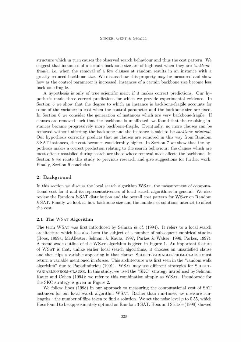
We studied the relationship between the number of solutions and the WSat cost withbackbone size controlled at different values. Figure 6 shows a log-log plot of the number ofsolutions against cost, where m/n is 4.29 and backbone size is 0.1n. A linear least squaresregression (lsr) fit is superimposed. Table 1 gives summary data on the log-log scatter plotfor different backbone sizes through the transition : the gradient and intercept of lsr fits,the product-moment correlation r and the rank correlation.

The number of solutions is strongly and negatively related to the cost for smaller back-bone sizes through the transition and the strength of the relationship is fairly constant asm/n is varied. We speculate that the strong relationship on these instances arises because

243


m/n Backbone Intercept Gradient r Rank corr.size of lsr fit of lsr fit

4.03 0.1n 3.8993 −0.1967 −0.7808 -0.77310.5n 4.1410 −0.2123 −0.6761 -0.66990.9n 4.2070 −0.1372 −0.1307 -0.1365

4.11 0.1n 3.8727 −0.1989 −0.7696 -0.76690.5n 4.1551 −0.2304 −0.6834 -0.68550.9n 4.1387 −0.1336 −0.1275 -0.1291

4.18 0.1n 3.7867 −0.1911 −0.7664 -0.77600.5n 4.0533 −0.2180 −0.6932 -0.69740.9n 4.0202 −0.1146 −0.1159 -0.1217

4.23 0.1n 3.7771 −0.1932 −0.7829 -0.78730.5n 3.9890 −0.2140 −0.6729 -0.68670.9n 3.9891 −0.1270 −0.1317 -0.1329

4.29 0.1n 3.7309 −0.1910 −0.7787 -0.78440.5n 3.9169 −0.2076 −0.6921 -0.69410.9n 3.7836 −0.0610 −0.0612 -0.0534

4.35 0.1n 3.6981 −0.1896 −0.8007 -0.79940.5n 3.8933 −0.2133 −0.6872 -0.69670.9n 3.8173 −0.1018 −0.1044 -0.0903

4.41 0.1n 3.6083 −0.1782 −0.7784 -0.76280.5n 3.8445 −0.2094 −0.7024 -0.70850.9n 3.7772 −0.1120 −0.1179 -0.1045

4.49 0.1n 3.5483 −0.1748 −0.7972 -0.79320.5n 3.7577 −0.2043 −0.6954 -0.69910.9n 3.6228 −0.0842 −0.0992 -0.0783

Table 1: Data on log-log correlations between number of solutions and cost with n = 100,m/n varied and backbone size fixed at different values.

244


102

103

104

105

106

107

108

102

103

104

number of solutions

cost

m/n = 4.29, backbone size = 0.1 n

Figure 6: Scatter plot of number of solutions and cost with n = 100, m/n = 4.29 andbackbone size fixed at 0.1n.

finding the backbone is straightforward and the main difficulty is encountering a solutiononce the backbone has been satisfied. The density of solutions in the region satisfying thebackbone is then important. For larger backbone sizes, the number of solutions is lessrelevant to the cost. No significant change in the number of solutions for large backboneinstances was observed as m/n was varied. That the number of solutions and the cost arenot strongly related for these instances is unsurprising, as the large backbone size impliesthat the solutions lie in a compact cluster and local search’s main difficulty is finding thiscluster (i.e. satisfying the backbone). Therefore we expect that the density of solutionswithin the cluster is not so important. Hoos (1998) observed that the correlation betweennumber of solutions and local search cost becomes small in the overconstrained region. Thiscan now be explained simply by the fact that the large-backbone instances dominate in thisregion.

3. Search Behaviour: the Hamming Distance to the Nearest Solution

In order to suggest the cause of the cost decay for large-backbone instances which wasobserved in Section 2.3, we made a detailed study of WSat’s search behaviour, i.e. theassignments visited during search. We report on this exploratory part of the research in

245


this section. We explain the somewhat novel search behaviour metrics which were usedbefore giving results and our discussion of them.

3.1 Definitions and Methods

Assuming a local search algorithm is PAC, in any given run of unlimited length, fb, thenumber of flips taken to find the first assignment where at most b clauses are unsatisfied, iswell-defined for b ≥ 0. f0 is then equal to the run length.

A particular run of a local search algorithm then consists of a series of assignmentsT0, T1, ..., Tf0 , where Ti is the assignment visited after i flips have been made. We found thaton Random 3-SAT with n = 100, an assignment satisfying all but a few clauses was quicklyfound and that during the remainder of the search, few clauses (1 - 10) were unsatisfied.As shown by Gent and Walsh (1993) in GSat, there is a rapid hill-climbing phase, which isalso suggested by Hoos (1998), followed by a long plateau-like phase in which the numberof unsatisfied clauses is low but constantly changing. In our experiments we used f5 as anarbitrary indicator of the length of the hill-climbing phase. Unlike in GSat, in WSat thereis no well-defined end point for the hill-climbing phase, since short bursts of hill-climbingcontinue to occur for the rest of the search. We think that using fb as the indicator withany value of b between 1 and 10 would give similar results.

Local search proceeds by flipping variable values and so we might expect that the Ham-ming distance between the current assignment and the nearest solution may also be ofinterest. The Hamming distance between two assignments hd(T1, T2) is simply the numberof variables which T1 and T2 assign differently. We studied the Hamming distance betweenthe current assignment T and the solution Tsol of C for which hd(T, Tsol) is minimised. Weabbreviate this hdns(T,C) (Hamming distance to nearest solution). For any assignmentT , hdns(T,C) may be calculated by using a complete SAT procedure which is modified sothat every solution to C is visited and its Hamming distance from T calculated.

3.2 Results

In this section, data is based on Random 3-SAT instances with n = 100 and backbone sizecontrolled at various values between 0.1n and 0.9n. Recall that to control backbone ata certain value, we generate satisfiable Random 3-SAT instances as usual and discard allthose whose backbone is not of the required size. We varied m/n from the point of 90%satisfiability (4.03) to the point of 20% satisfiability (4.49). hdns(Tf5 , C) is the Hammingdistance between the first assignment at which no more than 5 clauses are unsatisfied andthe nearest solution. For each instance we calculated the median value for f5 and the meanvalue for hdns(Tf5 , C) based on 1000 runs of WSat. In the plots in Figures 7 and 8, eachpoint is the median of 1000 instances.

Figure 7 shows the effect of varying m/n on f5 when backbone size is controlled. Thevalues for f5 are low compared to the cost and the range is very small. So although thecost to find a solution varies considerably from instance to instance, quasi-solutions arequickly found no matter what the overall cost. However, there are some notable effects ofbackbone size and m/n on f5. As might be expected, on the larger backbone instances, forwhich overall cost is generally higher, WSat takes slightly longer to find a quasi-solution.The effect of m/n is unexpected. If backbone size is controlled at 0.5n or more, as m/n is

246


increased WSat takes slightly longer to find a quasi-solution, although simultaneously costis decreasing as we have seen in Figure 4.

4 4.05 4.1 4.15 4.2 4.25 4.3 4.35 4.4 4.45 4.580

90

100

110

120

130

140

150

160

170

m/n

f 5

backbone size = 0.9 nbackbone size = 0.7 nbackbone size = 0.5 nbackbone size = 0.3 nbackbone size = 0.1 n

Figure 7: The effect of varying m/n on f5 while backbone size is controlled.

Figure 8 shows the effect of varying m/n on hdns(Tf5 , C) when the effects of backbonesize are controlled for. In this plot, the bars give the interquartile range. The spread ofvalues for mean hdns(Tf5 , C) at each point is also small relative to the effect of varyingm/n. Again the positive effect of backbone size on hdns(Tf5 , C) is as one might expectsince backbone size affects cost.

With backbone size controlled, as m/n is increased through the satisfiability threshold,mean hdns(Tf5 , C) decreases linearly for a wide range of backbone values. Hence, althougha quasi-solution (Tf5) is usually quickly found, on the instances of lower m/n this quasi-solution is considerably Hamming-distant from the nearest solution. As m/n is increased,while the backbone size is controlled, this effect is gradually lessened.

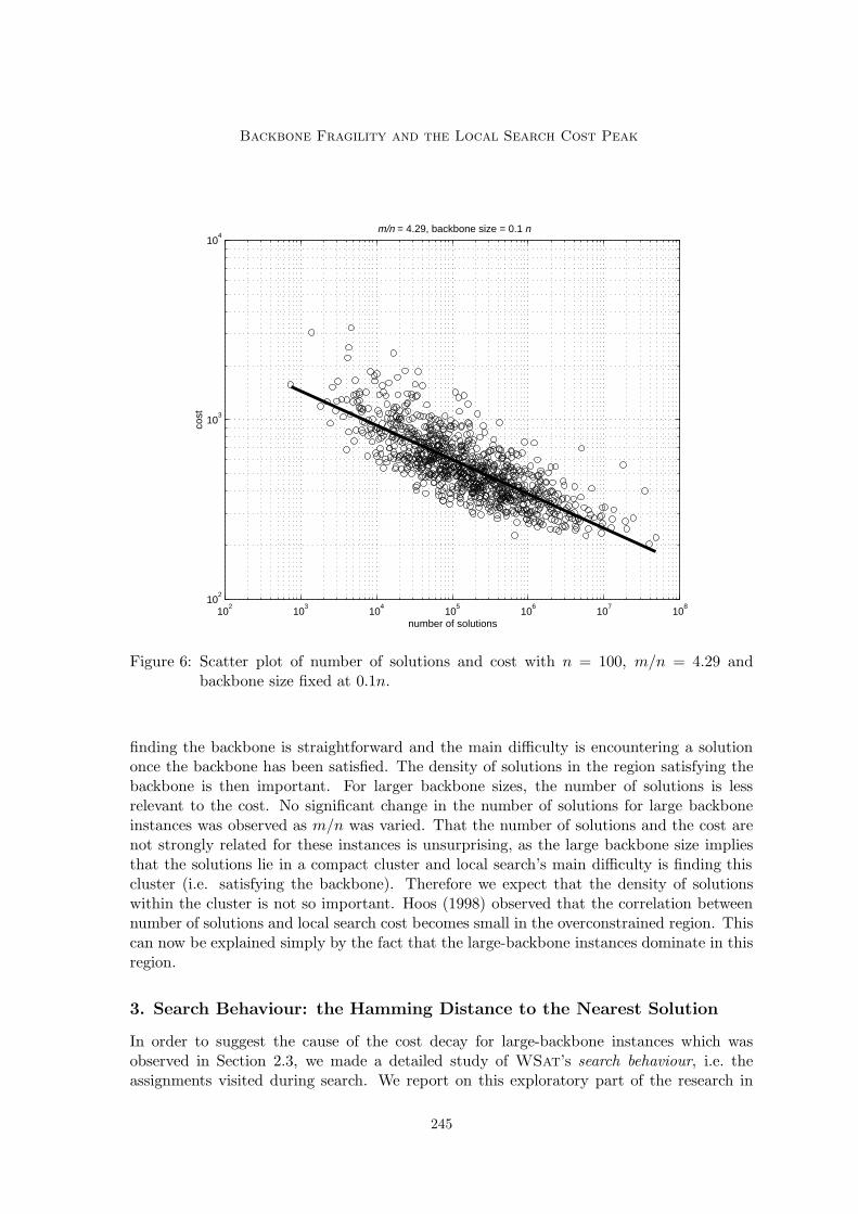
We also looked at the relationship between the search behaviour and the cost whenm/n was fixed and the backbone size was controlled. We found that in this case variancein hdns(Tf5 , C) accounts for most of the cost variance. Figure 9 shows a plot of the meanhdns(Tf5 , C) against the cost with backbone size controlled at 0.5n and m/n fixed at 4.29.An lsr fit is superimposed. The plot suggests hdns(Tf5 , C) is linearly related to log of cost.

Table 2 gives the intercept and gradient for lsr fits and r values with backbone sizecontrolled at three values and m/n varied. Variance in hdns(Tf5 , C) accounts for most ofthe variance in cost at three different backbone sizes and this is consistent through the

247


4 4.05 4.1 4.15 4.2 4.25 4.3 4.35 4.4 4.45 4.515

20

25

30

35

40

45

m/n

hdn

s(T

f 5,C)


Figure 8: The effect of varying m/n on hdns(Tf5 , C) while backbone size is controlled.

threshold. The scatter plots (not shown) and linear lsr fits to the data were similar inshape to that of Figure 9 and so are consistent with a linear relationship. The r values aregreatest for small-backbone instances but the reasons for this are unclear. Possibly, sincethe search is shorter on the small-backbone instances, success follows quickly after f5 andso hdns(Tf5 , C) is a better indicator of the likelihood of finding a solution.

Figure 8 showed that while backbone size is controlled, hdns(Tf5 , C) falls linearly as m/nis increased. The gradient of the fall is about −14. Table 2 showed that if backbone size iscontrolled and m/n fixed, hdns(Tf5 , C) is linearly related to log of cost, with the gradientof the fit being around 0.08. Given that this linear relationship continues to hold with aconstant gradient as m/n is varied (in fact the gradient decreases slightly) and assumingthat increasing m/n is not affecting the cost by other means, we would expect a lineardecrease in log of mean cost with gradient −1.12, which is only slightly steeper than theobserved decrease in log of median cost shown in Figure 4.

So the results are consistent with the idea that whatever factor causes the cost to decayexponentially as m/n is varied does so largely by causing hdns(Tf5 , C) to fall linearly.

3.3 Discussion

We have identified a pattern in search behaviour which is strongly related to the patternin cost discussed in Section 2.3. Our interpretation of this pattern is as follows. In each

248


m/n Backbone size Intercept Gradient rof lsr fit of lsr fit

4.03 0.1n 1.0528 0.0844 0.94450.5n 0.6928 0.0925 0.87690.9n 0.7065 0.0895 0.7308

4.11 0.1n 1.0166 0.0868 0.95110.5n 0.6315 0.0955 0.88520.9n 0.8158 0.0867 0.7196

4.18 0.1n 1.0858 0.0839 0.95560.5n 0.8090 0.0895 0.87990.9n 0.8109 0.0864 0.7195

4.23 0.1n 1.1290 0.0821 0.95810.5n 0.8343 0.0887 0.89740.9n 0.7480 0.0878 0.7691

4.29 0.1n 1.1289 0.0826 0.95500.5n 1.0032 0.0828 0.89350.9n 0.8382 0.0856 0.7579

4.35 0.1n 1.1664 0.0811 0.96280.5n 0.9835 0.0842 0.89960.9n 0.9835 0.0808 0.7728

4.41 0.1n 1.2029 0.0795 0.95650.5n 1.0274 0.0830 0.91350.9n 1.1070 0.0768 0.7816

4.49 0.1n 1.2458 0.0777 0.96610.5n 1.1472 0.0787 0.91970.9n 1.1930 0.0742 0.8086

Table 2: Data on correlations between hdns(Tf5 , C) and log10 cost with n = 100 and m/nand backbone size fixed at different values.

249


16 18 20 22 24 26 28 30 32 34 3610

2

103

104

105

hdns(Tf5

,C)

cost

Figure 9: The relationship of hdns(Tf5 , C) to log of cost when backbone size is controlledat 0.5n and m/n is fixed at 4.29.

instance the quasi-solutions which WSat visits form interconnected areas of the search spacesuch that local search can always move to a solution from them, without often moving to anassignment where many clauses are unsatisfied. The evidence for this is simply that WSat

runs are apparently always successful but visit the assignments where more clauses areunsatisfied very infrequently. Frank, Cheeseman and Stutz (1997) also mentioned in theiranalysis of GSat search spaces that in Random 3-SAT, local minima where few clauseswere unsatisfied can usually be escaped by unsatisfying just one clause.

We believe that in instances of higher cost this quasi-solution area extends to parts of thesearch space which are Hamming-distant from solutions, whereas in instances of lower costthe area is less extensive. The mean Hamming distance between the early quasi-solutionTf5 and the nearest solution is an accurate indicator of how extensive the quasi-solutionarea is. This interpretation suggests why hdns(Tf5 , C) is so strongly correlated with cost:the extensiveness of the quasi-solution area determines how costly it is to search. It alsosuggests why, on instances of higher cost, quasi-solutions are found slightly more quickly:when the quasi-solution area is extensive, from a random starting point a shorter series ofhill-climbing flips is required to find a quasi-solution.

250


The mean hdns(Tf5 , C) decreases linearly as m/n is increased while backbone size iscontrolled. At the same time, cost decays exponentially. We think this is because as m/nis increased, the quasi-solution area becomes progressively less extensive.

4. A Causal Hypothesis

The pattern in search behaviour from Section 3 and our interpretation of it suggested acausal hypothesis to account for the decay in cost discussed in Section 2.3 and hence theoverall peak. The key to this hypothesis is a property of SAT instances: backbone fragility.This property is qualitatively consistent with the above observations. Most importantly,although backbone fragility has implications for an instance’s search space topology, it isa property based on the logical structure of the SAT instance. In this section we motivateand define backbone fragility, discuss how it may be measured and show how it relates tothe patterns reported in Sections 2.3 and 3.

4.1 Backbone Fragility : Motivation

Suppose B is a small sub-bag of the clauses of a satisfiable SAT instance C, such thatthere exists a set of quasi-solutions QB where at most the clauses B are unsatisfied. Whatstructural property of C would cause the quasi-solutions QB to be attractive to WSat?We already know that if the backbone of a Random 3-SAT instance is small, its solutionsare found with little search (Parkes, 1997). The solutions to C −B (C −B denotes C withone copy of each member of B removed) are either solutions to C or members of QB. Ifwe assume that the assignments which are attractive to WSat on C are approximatelythe same assignments which are attractive on C − B, then the members of QB (which aresolutions of C−B) will be attractive in C when the backbone of C−B is small, particularlyif C’s backbone is large. Furthermore for any TB ∈ QB, the number of variables which donot appear in the backbone of C−B is an upper bound on hdns(TB, C), so a large reductionin the backbone size allows for high hdns(TB, C). To summarise, if the removal of a certainsmall sub-bag of clauses causes the backbone size to be greatly reduced, we can expect thatquasi-solutions where only these clauses are unsatisfied will be attractive to WSat andpossibly Hamming-distant from the nearest solution.

We are interested in quasi-solutions in general rather than those in QB. If removing arandom small set of clauses on average causes a large reduction in the backbone size, wesay that the instance is backbone-fragile. Where the effect on the backbone is smaller onaverage, the instance is backbone-robust. If a large-backbone instance is backbone-fragile, byextension of the above argument we expect that in general quasi-solutions will be attractiveand they may be Hamming-distant from the nearest solution. Hence this idea is consistentwith our observations and interpretation in Section 3: backbone fragility approximatelycorresponds to how extensive the quasi-solution area is.

The idea that backbone fragility is the underlying factor causing the search behaviourpattern is appealing for other reasons. For each entailed literal l of C, there must be asub-bag of clauses in C whose conjunction entails l. For any given backbone size, as clausesare added, for any given entailed literal l we expect that the extra clauses allow alternativecombinations of clauses which entail l. Hence after adding clauses whilst controlling thebackbone size, the random removal of clauses will have less effect on the backbone since

251


the fact that a literal is entailed depends less on the presence of particular sub-bags. Asclauses are added, we expect that instances will become less backbone-fragile. Given thehypothetical relationship between backbone fragility and the search behaviour, this wouldthen explain qualitatively why the search behaviour changes as it does when m/n is varied.We think that because backbone fragility is a property of the instance’s logical structure, itsstudy may also lead to further results about complexity issues, but we postpone discussionof this until Section 8.

4.2 The Measurement of Backbone Robustness

We now define a measure of the backbone robustness of an instance which will allow us totest predictions of the hypothesis. We take the instance C and delete clauses at random,halting the process when the backbone size is reduced by at least half. At this point werecord as the result the number of deleted clauses. This constitutes one robustness trial.Our metric for backbone robustness is the mean result of all such possible trials, i.e. theaverage number of random deletions of clauses which must be made so as to reduce thebackbone size by half.

It is infeasible to compute the results of all possible robustness trials. Therefore, whenmeasuring backbone robustness of an instance we estimated it by computing the average ofa random sample of trials. We used at least 100 robustness trials in each case and in orderto ensure a reasonably accurate estimate, we continued to sample more robustness trialsuntil the standard error was less than 0.05 × the sample mean (in which case our estimateof the mean was accurate to within about 10% at the 95% confidence level). With n = 100,using satisfiable instances from near the satisfiability threshold whose backbone size wascontrolled at 50, usually less than 250 robustness trials were required for the estimate toconverge in this way. Even then, backbone robustness was costly to compute.

There were different possible metrics for backbone fragility/robustness, but we foundthat the metric described above gave the clearest results for our purposes without an unne-cessarily complicated definition. Other metrics, such as the reduction in backbone size whena random fixed fraction of clauses are removed, may be more suitable in other contexts.

4.3 The Change in Backbone Robustness as the Control Parameter is Varied

As discussed in Section 4.1 we expect that if backbone size is controlled, backbone robustnessincreases as m/n is increased. Since our measure of backbone robustness is defined in termsof the size of the backbone, it is most useful when comparing instances of equal backbonesize.

We found that increasing the control parameter made instances more backbone-robust,as expected. Figure 10 shows the effect on backbone robustness of increasing m/n throughthe satisfiability threshold while n = 100 and backbone size is controlled. Each point is themedian of 1000 instances.

We note that backbone robustness as defined by our measure is generally higher forinstances with larger backbones. We think that this is because on the large-backboneinstances, the backbone must be reduced by a larger number of literals in each fragility trialand that this requires more clauses to be removed.

252


4 4.05 4.1 4.15 4.2 4.25 4.3 4.35 4.4 4.45 4.54

6

8

10

12

14

16

18

20

22

m/n

back

bone

rob

ustn

ess


Figure 10: Backbone robustness through the satisfiability transition, with backbone sizefixed at 0.1n 0.5n and 0.9n.

5. A Correct Prediction about Cost Variance

We may assert that the fall of cost observed with the increase in the control parameteris due to the change in some other factor F , as for example Yokoo (1997) has. Such anassertion makes an important and testable prediction: that any variation in F when thecontrol parameter is fixed accounts for some of the variation in cost. However there maybe other factors whose influence on the cost is so great as to obscure the effect of F whenthe control parameter is fixed. To best reveal the effect of F , if there is any, the effects ofsome other factors may have to be controlled for.

Backbone robustness is our proposed factor F . The backbone size is another factorwhich strongly influences the cost. Our result in this section is that when the effects ofm/n and backbone size are controlled for, i.e. when they are fixed, the effects of backbonerobustness can be seen quite clearly for large-backbone instances.

5.1 Correlation Data

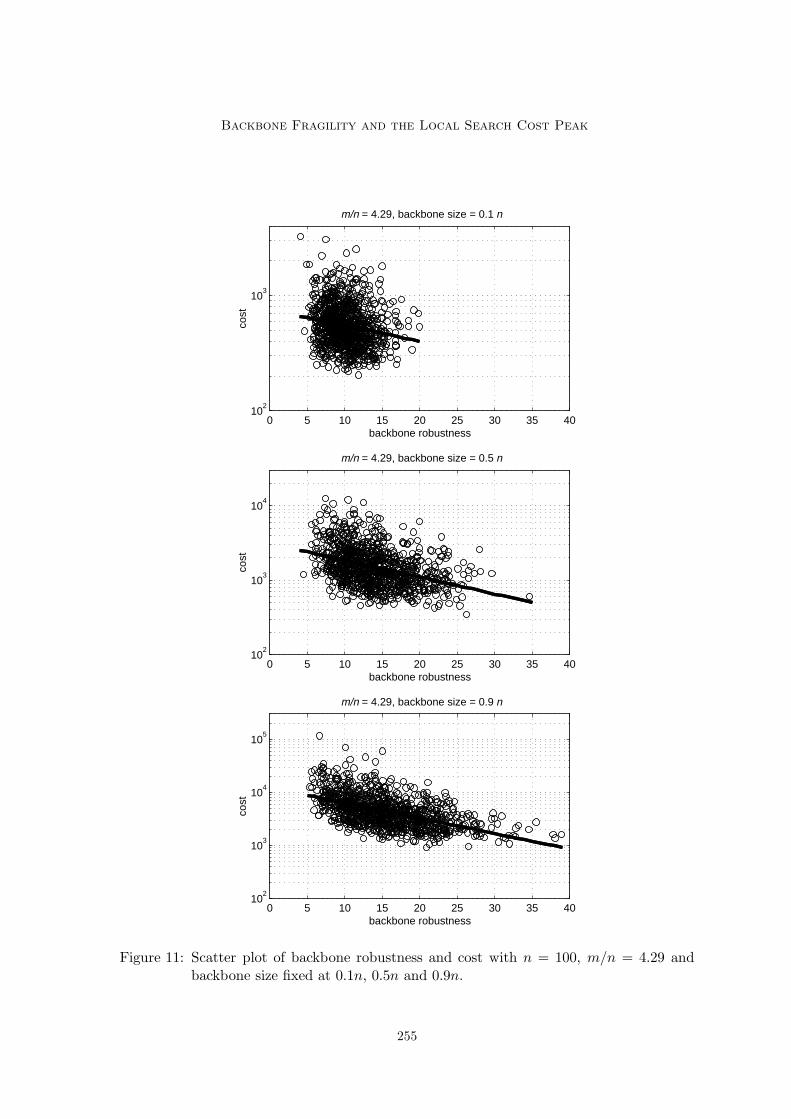
Figure 11 shows a plot of the log cost against the measure of backbone robustness forRandom 3-SAT instances with n = 100, m/n 4.29 and backbone size controlled at 0.1n,0.5n and 0.9n. A linear lsr fit is superimposed in each case. Table 3 gives the intercept,

253


m/n Backbone size Intercept Gradient r r−95% r+95% Rank corr.of lsr fit of lsr fit coefficient

4.03 0.1n 3.0338 −0.0204 −0.1928 −0.2506 −0.1400 −0.19340.5n 3.7075 −0.0370 −0.3730 −0.4191 −0.3235 −0.37130.9n 4.2846 −0.0419 −0.4711 −0.5165 −0.4251 −0.4699

4.11 0.1n 2.9639 −0.0134 −0.1490 −0.2088 −0.0873 −0.14020.5n 3.6675 −0.0351 −0.3891 −0.4355 −0.3417 −0.37700.9n 4.2287 −0.0370 −0.4535 −0.5001 −0.4065 −0.4662

4.18 0.1n 2.9365 −0.0146 −0.1745 −0.2356 −0.1149 −0.16630.5n 3.6067 −0.0302 −0.3840 −0.4272 −0.3389 −0.37380.9n 4.1811 −0.0338 −0.5306 −0.5687 −0.4921 −0.5466

4.23 0.1n 2.9257 −0.0155 −0.2107 −0.2659 −0.1553 −0.21160.5n 3.5142 −0.0239 −0.3643 −0.4105 −0.3154 −0.34360.9n 4.1313 −0.0312 −0.5253 −0.5645 −0.4818 −0.5457

4.29 0.1n 2.8766 −0.0136 −0.1894 −0.2483 −0.1300 −0.20530.5n 3.4903 −0.0225 −0.3863 −0.4350 −0.3395 −0.39960.9n 4.0934 −0.0290 −0.5325 −0.5721 −0.4931 −0.5467

4.35 0.1n 2.8261 −0.0109 −0.1671 −0.2250 −0.1105 −0.17240.5n 3.4325 −0.0199 −0.3734 −0.4222 −0.3244 −0.37820.9n 3.9939 −0.0237 −0.4984 −0.5394 −0.4555 −0.5243

4.41 0.1n 2.7925 −0.0100 −0.1763 −0.2321 −0.1175 −0.16830.5n 3.3772 −0.0172 −0.3452 −0.3954 −0.2919 −0.35820.9n 3.9284 −0.0211 −0.5152 −0.5582 −0.4692 −0.5270

4.49 0.1n 2.7164 −0.0073 −0.1392 −0.1926 −0.0841 −0.13550.5n 3.3506 −0.0170 −0.4034 −0.4585 −0.3516 −0.40270.9n 3.8720 −0.0198 −0.5549 −0.5949 −0.5125 −0.5604

Table 3: Data on the correlation between backbone robustness and log10 cost with n = 100and m/n and backbone size fixed at different values.

gradient and r values for lsr fits with backbone size controlled at the same three values andwith m/n varied through the threshold.

The r values suggest an effect of backbone robustness on cost, particularly for largebackbone sizes. For smaller backbone sizes, we imagine that finding the backbone is less ofan issue and so backbone fragility, which hinders this, has less of an effect. For the largerbackbone sizes, we think the main difficulty for WSat is satisfying the backbone; backbonefragility is then important. However, given the somewhat unclear shape of the scatter plots,there are several concerns as to the significance of the correlation, which we now addressusing some simple statistical methods.

254


0 5 10 15 20 25 30 35 4010

2

103

backbone robustness

cost


0 5 10 15 20 25 30 35 4010

2

103

104

backbone robustness

cost


0 5 10 15 20 25 30 35 4010

2

103

104

105

backbone robustness

cost


Figure 11: Scatter plot of backbone robustness and cost with n = 100, m/n = 4.29 andbackbone size fixed at 0.1n, 0.5n and 0.9n.

255


5.2 An Artifact of the Distributions of the Variables?

One concern is that the observed r could also have arisen simply because of the distributionsof the two variables rather than because of any relationship between them. This is a seriousconcern here as the distributions are unknown.

The null hypothesis, H0 is that the value of r which results from the distributions of thetwo variables is equal to the observed r. A randomisation method can be used to test H0.See Appendix A for details of this method. For each data set presented, 1000 randomisedpairings of the data were constructed. In each case, we found that the observed r doesnot fall within the range of the sampling distribution of r for randomised pairings. H0 cantherefore be rejected at the 99.9% confidence level.

The r coefficient, given above, can be greatly affected by outliers. Therefore the rankcorrelation coefficient, which is less affected, was also calculated. The rank correlation isalso given in Table 3. We found that in each case the rank correlation coefficient is notconsiderably different from the r coefficient. This demonstrates that the observed r was notgreatly affected by outliers.

5.3 Confidence Intervals for the Correlation

Given that there is a relationship between the two variables which is not merely an artifactof the distributions or of outliers, how accurate is our measurement of r? A bootstrapmethod can be used to obtain bounds on a confidence interval for this statistic. Again, thereader is referred to Appendix A for details of this method. Using this method with 1000pseudo-samples we obtained lower and upper bounds on the 95% confidence interval for r,which are also given in Table 3 as r−95% and r+95% respectively. The data implies with 95%confidence, the upper bounds on the amount of error in our estimates of r2 are betweenabout 0.02 and 0.05.

6. A Correct Prediction about Very Backbone-Fragile Instances

Our hypothesis proposes that high backbone fragility of instances quite accurately representsthe factor which (via the search behaviour patterns uncovered in Section 3) causes highWSat cost for those instances. However, it is plausible that the high backbone fragility isa by-product of some unmeasured latent factor and that it is not causally related to thecost.

To help establish the causal link between backbone fragility and cost, we therefore cre-ated sets of random SAT instances which had higher backbone fragility than usual Random3-SAT instances. This is to some degree following the methodological precedent of Bayardoand Schrag (1996), who created random instances which contained small unsatisfiable sub-instances but which had few constraints overall. These were often found to be exceptionallyhard for the complete procedure Ntab. Their experiments thereby helped establish thatthis feature of instance structure was the cause of exceptionally high cost for completeprocedures.

We cannot easily set backbone fragility directly, since it is not a generation parameter.One manipulation experiment which is possible is the use of an instance generation proced-ure which results in instances with a higher backbone fragility. Our hypothesis predicts that

256


instances generated using such a procedure will be harder than Random 3-SAT instances.In this section we define such a procedure and test the prediction. It may be that our pro-cedure is also manipulating the latent factor. However, since the procedure is specificallydesigned to increase backbone fragility, a correct prediction here still lends credibility toour hypothesis.

6.1 Backbone-minimal Sub-instances

Suppose we have a SAT instance C and we remove a clause such that the backbone is notaffected by the removal of the clause. If such clauses are repeatedly removed, eventuallythe instance will be such that no clause can be removed without disturbing the backbone.In this case we have a backbone-minimal sub-instance (BMS) of C. More formally, we havethe following definition:

Definition A SAT instance C ′ is a BMS of C iff

• C ′ is a sub-instance of C (i.e. a sub-bag of the clauses) such that C ′ has the samebackbone as C.

• for each clause c of C ′ there exists a literal l such that:

1. C ′ → l

2. (C ′ − {c}) ∧ ¬l is satisfiable

i.e. every strict sub-instance of C ′ has a strictly smaller backbone than the back-bone of C ′ 2

BMSs can be seen as satisfiable analogues of the minimal unsatisfiable sub-instances(MUSs) of unsatisfiable instances studied by amongst others Culberson and Gent (1999b)in the context of graph colouring and Gent and Walsh (1996) and Bayardo and Schrag(1996) in satisfiability. An MUS of an instance C is a sub-instance which is unsatisfiable,but such that the removal of any one clause from the sub-instance renders it satisfiable.Just as all unsatisfiable instances must have an MUS, all satisfiable SAT instances musthave a BMS. Having a BMS does not depend on having a non-empty backbone – if thebackbone of the instance is empty, its BMS is the empty sub-instance. An instance canhave more than one BMS. Different BMSs of an instance may share clauses. One BMS ofan instance cannot be a strict sub-instance of another.

Suppose the backbone of a satisfiable instance C is the set of literals {l1, l2, . . . , lk}. Letd be the clause ¬l1 ∨ ¬l2 ∨ . . . ∨ ¬lk. Then we have the following useful fact:

Theorem C ′ is a BMS of C iff C ′ ∧ d is an MUS of C ∧ d 2

A simple proof of the above is given in Appendix B. Due to this fact, methods for studyingMUSs can be applied to the study of BMSs. We can study the BMSs of a satisfiableinstance C by finding the backbone of C and then studying the MUSs of C ∧ d: each ofthese corresponds to a BMS of C since d must be present in every MUS of C ∧ d.

To find a BMS of C we determine the backbone, then find a random MUS of C∧d usingthe same MUS-finding method as Gent and Walsh (1996) and remove d from the result.

257


Instances Backbone robustness10th percentile Median 90th percentile

Preserve-backbone(C, 0, C ′) 8.5845 12.9700 20.6300Preserve-backbone(C, 5, C ′) 7.7374 12.0317 19.1700Preserve-backbone(C, 10, C ′) 7.1977 11.0851 17.3500Preserve-backbone(C, 20, C ′) 6.0690 9.3913 14.5351Preserve-backbone(C, 40, C ′) 4.2622 6.4899 9.9900Preserve-backbone(C, 80, C ′) 2.0745 2.8661 3.9851BMS 1.0200 1.0600 1.1600

Table 4: The effect of Preserve-backbone on backbone robustness.

6.2 Interpolating Between an Instance and one of its BMSs

Once a BMS C ′ has been established, we can also study the effects of interpolation betweenC and C ′ by removing at random from C some of the clauses which do not appear inC ′. This is equivalent to removing clauses at random such that the backbone is preserved.Preserve-backbone(C, mr, C ′) will denote C with mr clauses, which do not appear inthe BMS C ′, removed at random. The resulting instance will have the same backbone asC.

Just as increasing m/n while controlling the backbone size causes backbone robustnessto increase, we have found that deleting clauses such that the backbone is unaffected causesbackbone robustness (as measured above) to decrease, as one might expect.

We used 500 Random 3-SAT instances with n = 100 and m/n = 4.29. For each instancewe found one BMS. We then used Preserve-backbone to interpolate with mr set atvarious values. Table 4 shows the effect of increasing mr on backbone robustness. TheBMSs of the threshold instances are so backbone-fragile that the removal of just one clausefrom them is likely to reduce the backbone by a half or more.

Our hypothesis predicts that as this interpolation from C to C ′ proceeds, the costfor local search increases because the backbone robustness decreases. It is conceivable,although it would be very surprising, that removing any clauses from random instancesnear the threshold generally makes their cost for local search increase. If this were thecase, any increase in cost during interpolation towards a BMS could merely be due to theremoval of clauses per se rather than the removal of clauses whilst preserving the backbone.To control for this possibility we also removed clauses according to two other procedures.The procedure Random(C, mr) removes mr clauses from C at random. The procedureReduce-backbone(C, mr) removes mr clauses such that each time a clause is removed,the size of the backbone is reduced. The clause to be removed is chosen randomly from allsuch clauses. This procedure therefore uses the opposite removal criterion to Preserve-

backbone. If the backbone becomes empty, no further clauses are removed.Figure 12 shows the effect on per-instance cost of applying the three clause removal

procedures to the same set of 500 Random 3-SAT threshold instances. Each plot is themedian per-instance cost.

258


0 10 20 30 40 50 60 70 8010

2

103

104

mr

cost

Preserve−backboneReduce−backboneRandom

Figure 12: The effect of the three clause removal procedures on median per-instance cost.

We observe that removing clauses randomly or such that the backbone is strictly re-duced, causes cost to be reduced, so the removal of clauses does not in itself cause highercost. The Reduce-backbone procedure causes a greater initial fall in cost, as the back-bone size is reduced more quickly than with Random. However, the cost then stabilises forReduce-backbone because the backbone becomes empty and thereafter no more clausesare removed.

Removing clauses according to Preserve-backbone causes the local search cost toincrease by an amount approximately exponential in the number of clauses removed. Table5 gives more data on this effect and also cost data for BMSs. The interpolation shifts thewhole distribution up, not just the median. The median cost of the BMSs, which are themost backbone-fragile of all the instances, is more than three times that of the 90th costpercentile of Random 3-SAT instances.

The BMSs of these instances had between 254 and 318 clauses. The above resultstherefore demonstrate the existence of instances in the underconstrained region which aremuch harder than the typical instances from near the satisfiability threshold. However sincethese were not obtained by sampling from Random 3-SAT directly, we do not know howoften they occur. As far as we know, they are vanishingly rare and therefore, in contrastto exceptionally hard instances for complete algorithms, it seems unlikely that they affectthe mean cost. Also, while Gent and Walsh (1996) showed that the exceptionally hard

259


Instances Per-instance cost10th percentile Median 90th percentile

Preserve-backbone(C, 0, C ′) 517 1450 5175Preserve-backbone(C, 5, C ′) 537 1515 5657Preserve-backbone(C, 10, C ′) 557 1608 6009Preserve-backbone(C, 20, C ′) 570 1803 7037Preserve-backbone(C, 40, C ′) 643 2295 10683Preserve-backbone(C, 80, C ′) 816 4154 24313BMS 1556 16945 135883

Table 5: The effect of Preserve-backbone on per-instance cost.

instances for complete algorithms are hard for a different reason from that of thresholdinstances, BMSs are apparently hard for the same reason – because they are backbone-fragile.

One useful by-product of this section is a means of generating harder test instances forlocal search variants without increasing n. However these instances do require O(m + n)complete searches to generate: O(n) to determine satisfiability and the backbone and O(m)to reduce to a BMS.

7. A Correct Prediction about Search Behaviour

Recall that in the motivating discussion of Section 4.1 it was suggested that the quasi-solutions in QB would be attractive if the backbone of C−B was small. That is to say thatthe clauses of B are more likely to be the set of unsatisfied clauses if the removal of theclauses of B has a large effect on the backbone. This part of the hypothesis also makes aprediction about search behaviour – that clauses most often unsatisfied by WSat should bethose whose removal reduces the backbone size most. In this section we show this predictionto be correct.

We looked at individual instances which were cost percentiles from a set of 5000 Randomk-SAT instances with n = 100 and m/n = 4.29. Per-instance cost was determined as inprevious sections. For each clause in the instance, we calculated the number of backboneliterals which were no longer entailed if the clause was removed. This is a simple measure ofthe backbone contribution (bc) of the clause – how much the backbone size depends on thepresence of the clauses. If a clause’s backbone contribution is high, it is termed a backbone-critical clause. We made 1000 runs of WSat on each instance under the same conditions asin previous sections. During search, each time the current assignment changed we recordedwhether each clause was unsatisfied. The result of averaging the number of times the clausewas unsatisfied over all runs gives the unsatisfaction frequency (uf) of that clause.

Figure 13 shows a plot of these two quantities for the clauses of the instance whose costwas median of 5000 threshold instances. We note from this figure that the clauses whosepresence contributes the most to the backbone are more often unsatisfied than averageduring WSat search.

260


0 5 10 15 20 2510

0

101

102

103

backbone contribution

unsa

tisfa

ctio

n fr

eque

ncy

Figure 13: Scatter plot of unsatisfaction frequency against backbone contribution for theclauses of the cost median of 5000 instances, m/n = 4.29, n = 100.

Table 6 confirms this pattern. Each row of the table gives data for one instance. Weselected cost percentiles; individual instances of varying degrees of difficulty. For examplethe row labelled ‘30th’ corresponds to the instance whose cost is the 1500th in rank fromthe easiest to the most difficult of the 5000 instances, while the 50th percentile instanceis the one used to produce Figure 13. The third and fourth columns give the mean andstandard deviation of the unsatisfaction frequency over all clauses in the instance and thelast two columns give the same statistics for the sub-bag of the clauses which were mostbackbone-critical (their backbone contribution was in the top 10%).

Table 7 shows that the converse effect is also present: the clauses which are most oftenunsatisfied (their unsatisfaction frequency is in the top 10%) are more backbone-critical thanaverage. Although an effect is quite clear from the means, there are sometimes particularlylarge standard deviations in bc values for the most frequently unsatisfied clauses. Thisis because, as can be seen from Figure 13, some clauses are very often unsatisfied eventhough removing them on their own does not affect the backbone size at all. We havefound in other experiments that the removal of these clauses along with other small randombags of clauses does on average reduce the backbone size considerably. The large standarddeviations therefore arise because the true backbone contribution of these clauses is notapparent when using this simple measure.

261


Cost Backbone All clauses Most backbone-Percentile size critical clauses

uf mean uf std. dev. uf mean uf std. dev.10th 16 11.3430 8.0704 20.8703 8.873020th 11 13.1079 10.9596 30.1817 16.873030th 13 21.0207 16.3680 41.4660 21.114240th 36 22.9825 21.3118 56.6841 27.466050th 48 29.5615 25.9275 72.0704 38.777960th 25 36.2940 35.6327 96.1664 54.308170th 63 52.4198 48.1078 119.7691 66.818780th 70 92.2623 87.7827 167.3428 149.805890th 93 108.3124 127.1968 306.7200 198.6933

Table 6: Unsatisfaction frequencies of clauses in different cost percentile instances.

Cost Backbone All clauses Most oftenPercentile size unsatisfied clauses

bc mean bc std. dev. bc mean bc std. dev.10th 16 0.5921 1.2358 2.0909 1.852920th 11 0.4848 1.0380 1.7727 1.963230th 13 0.3963 1.2405 1.8409 2.449040th 36 1.8089 4.2411 8.3182 6.462050th 48 1.0629 3.2781 6.3182 6.604360th 25 1.3800 3.4920 7.7500 5.779470th 63 3.3916 8.8630 14.9091 15.812680th 70 0.6946 3.4577 2.5909 7.860290th 93 3.0653 10.0376 16.9318 20.6436

Table 7: Backbone contributions of clauses in different cost percentile instances.

262


For instances of different costs at the satisfiability threshold, the clauses which are mostlikely to be unsatisfied during search have a higher backbone contribution than average.Conversely, the clauses which have the largest backbone contribution are more likely to beunsatisfied during search. This section therefore demonstrates that as well as explainingdifferences in cost between instances, the backbone fragility hypothesis can also explaindifferences in the difficulty of satisfying particular clauses during search.

8. Related and Further Work

Clark et al. (1996) showed that the number of solutions is correlated with search cost fora number of local search algorithms on random instances of different constraint problems,including Random 3-SAT. The pattern was confirmed by Hoos (1998) using an improvedmethodology. Clark et al.’s work was the first step towards understanding the variance incost when the number of constraints is fixed. We have followed their approach both bylooking at the number of solutions and by using linear regression to estimate strengths ofrelationships between factors.

Schrag and Crawford (1996) made an early empirical study of the clauses (includingliterals) which were entailed by Random 3-SAT instances. Parkes (1997), whose study isalso discussed in Section 1, looked in detail at backbone size in Random 3-SAT and its effecton local search cost. He also linked the position of the cost peak to that of the satisfiabilitythreshold by the emergence of large-backbone instances which occurs at that point. Parkesalso identified the fall in WSat cost for instances of a given backbone size. This wastherefore the basis for our study. Parkes conjectured that the presence of a “failed cluster”may be the cause of high WSat cost for some large-backbone Random 3-SAT instances.According to this hypothesis, the addition of a single clause could remove a group of solutionswhich is Hamming distant from the remaining solutions, reducing the size of the backbonedramatically. Such a clause would then have a large backbone contribution. Therefore ourexplanation for the general high cost of the threshold region has certain features in commonwith Parkes’ conjecture. In particular we agree that it is the presence of clauses with alarge backbone contribution which causes high cost. This is especially demonstrated by ourresults from Section 7.

Frank et al. (1997) studied in detail the topology of the GSat search space induced bydifferent classes of random SAT instances. Their study discussed the implications of searchspace structure for future algorithms, as well as the effects of these structures on algorithmssuch as GSat. They also noted that some local search algorithms such as WSat may beblind to the structures they studied because they search in different ways to GSat.

Yokoo (1997) also addressed the question of why there is a cost peak for local searchas m/n is increased. The approach was to analyse the whole search space of small sat-isfiable random instances. While in this study, we have only examined SAT, Yokoo alsoshowed his results generalised to the colourability problem. Yokoo used a deterministichill-climbing algorithm. He studied the number of assignments from which a solution isreachable (solution-reachable assignments) via the algorithm’s deterministic moves, whichlargely determines the cost for the algorithm.

We followed Yokoo in looking for a factor competing with the number of solutions whoseeffect on cost changes as m/n is increased. The factor which Yokoo proposed as the cause

263


of the overall fall in cost was the decrease in the number of local minima – assignmentsfrom which no local move decreased the number of unsatisfied clauses. The decrease inthis number was demonstrated as m/n is increased. The decrease was attributed to thedecreasing size of “basins” (interconnected regions of local minima with the same numberof unsatisfied clauses). Yokoo claimed (p. 363) that:

“adding constraints [...] makes the [instance] easier by decreasing the numberof local minima”.

However, we do not think it is clear a priori what the relationship between the numberof local minima and the cost is in a given instance and Yokoo did not study it sufficientlyto convince us of his explanation. In contrast with Yokoo, we have studied in detail therelationship between the backbone fragility of instances and WSat’s cost on these instancesand confirmed it by testing predictions of our hypothesis. Also, we studied instance proper-ties that related to the logical structure of the clauses rather than the search space topologywhich was induced as we think this has more potential to generalise across algorithms andeven to address complexity issues, as we explain towards the end of this section.

Hoos (1998) also analysed the search spaces of SAT instances in relation to local searchcost by looking at two new measures of the induced objective function which he defined,including one based on local minima. Although via these measures, Hoos was not able toaccount for the Random 3-SAT cost peak, he found that the features were correlated withcost for some SAT encodings of other problems and has also shown (Hoos, 1999b) that hismeasures can help distinguish between alternative encodings of the same problem.

How does the pattern we have uncovered fit in to other work on what makes instancesrequire a high cost to solve? Gent and Walsh (1996) looked at the probability that an unsat-isfiable SAT instance became satisfiable if a fixed number of clauses are removed at random.The unsatisfiable instances which had the highest computational cost for a complete pro-cedure were found to be those which were unsatisfiability-fragile – their unsatisfiability wassensitive to the random removal of clauses. It may therefore be that the fragility of an in-stance’s unsatisfiability or backbone size is the cause of high computational cost both in thecontext of complete procedures and incomplete local search, which would be an interestinglink between the two algorithm classes. This link may form the basis of a possible explan-ation of the reasons why threshold Random 3-SAT instances may be universally hard inthe average case, as opposed to merely costly for some class of algorithms. Recent work byMonasson et al. (1999a, 1999b) has suggested that parameterised distributions of instanceswhich are hard in the average case, e.g. Random 3-SAT, exhibit a discontinuity in thebackbone size3 as the control parameter is varied, whereas in polynomial time average-casedistributions, such as Random 2-SAT, the backbone size changes smoothly. They proposethat the complexity of the distribution is linked to the presence of this discontinuity. Weconjecture that this may be because in the asymptotic limit, instances which are backbone-or unsatisfiability-fragile only persist as n is increased where there is such a discontinuity.This line of research may therefore establish a testable causal mechanism for this pattern,showing how the properties of the instance distributions affect algorithm performance.

It would be interesting to compare backbone fragility in different random distributionsof 3-SAT instances, such as those introduced by Bayardo and Schrag (1996) and by Iwama,

3. Monasson et al.’s definition of the backbone also extends to unsatisfiable instances.

264


Miyano and Asahiro (1996) to see whether differences in local search cost could be explained.A method which generates satisfiable instances which are quickly solved by local search isanalysed by Koutsoupias and Papadimitriou (1992) and Gent (1998). Random clauses areadded to the formula as in Random 3-SAT but only if they do not conflict with a certainsolution which is set in advance. We conjecture that overconstrained examples of these arequickly solved by local search because they are very backbone-robust.

An interesting possibility mentioned by Hoos and Stutzle (1998) suggested by the expo-nential run length distribution, was that local search is equivalent to random generate-and-test in a drastically reduced search space. We conjecture that this reduced search spacecorresponds to the quasi-solution area. Measurements of hdns(TB, C) for quasi-solutionsTB may therefore be indicative of the extensiveness of this reduced search space, especiallysince this metric is linearly correlated with log cost. Further experimentation in this veinmay therefore reveal more about the topology of the reduced search space which could inturn lead to better local search algorithms designed to exploit this knowledge.

Finally, we should emphasise that the notions of backbone and backbone-fragility areequally applicable to non-random SAT instances. In future we may be able to confirm thatthe results we have shown for random SAT instances apply equally to benchmark and real-world SAT instances. However, one caveat here is that entailed literals may be uncommonin these instances and we may need to study the fragility of other sets of entailed formulas.

9. Conclusion

We have reconsidered the question of why cost for local search peaks near the Random3-SAT satisfiability threshold. The overall pattern is one of two competing factors. Thecause of the onset of high cost as the control parameter is increased has been previouslyestablished as the decreasing number of solutions. We have proposed that the cause of thesubsequent fall in cost is falling backbone fragility.

We found a striking pattern in the search behaviour of the local search algorithm WSat.For instances of a given backbone size, in the underconstrained region of the control para-meter, WSat is attracted early on to quasi-solutions which are Hamming-distant from thenearest solution. This distance is also very strongly related to search cost. As the controlparameter is increased, the distance decreases. We suggested backbone fragility was thecause of this pattern.

We defined a measure of backbone robustness. Backbone-fragile instances have lowrobustness. We were then able to test predictions of the hypothesis that the fall in backbonefragility is the cause of the overall decay in cost as the control parameter is increased. Wefound that the hypothesis made three correct predictions. Firstly that the degree to whichan instance is backbone-fragile is correlated with the cost when the effects of other factorsare controlled for. Secondly, that when Random 3-SAT instances are altered so as to bemore backbone-fragile (by removing clauses without disrupting the backbone) their costincreases. Thirdly, that the clauses most often unsatisfied during search are those whosedeletion has most effect on the backbone.

We now summarise our interpretation of the evidence. In the underconstrained region,instances with small backbones are predominant. In this region, the rapid hill-climbingphase typically results in an assignment which is close to the nearest solution (and probably

265


satisfies the backbone). Since finding the small backbone is largely accomplished by hill-climbing, typical cost for WSat is low in this region and variance in cost is due to variancein the density of solutions in the region of the search space where the backbone is satisfied.

In the threshold region, large-backbone instances quickly appear in large quantities.For large-backbone instances, the main difficulty for local search is to identify the backbonerather than to find a solution once the backbone has been identified. The identification of alarge backbone may be accomplished by the rapid hill-climbing phase to a greater or lesserextent. We think that this extent is determined by the backbone fragility of the instance.If a large-backbone instance is backbone-fragile the hill-climbing phase is ineffective andresults in an assignment which is Hamming-distant from the nearest solution (probablyimplying that much of the backbone has not been identified). Then a costly plateau searchis required to find a solution. Hence when the rare large-backbone instances do occur in theunderconstrained region, they are extremely costly to solve because of their high backbonefragility.

If a large-backbone instance is more backbone robust, the rapid hill-climbing phase ismore effective in determining the backbone and the plateau phase is shorter. So overallthe instance is less costly for WSat to solve. Hence for large-backbone instances, sincebackbone fragility increases as we add clauses, cost decreases. In the overconstrained region,large backbone instances are dominant and so backbone fragility becomes the main factordetermining cost. Hence cost decreases in this region. Our hypothesis proposes the followingexplanation for the cost peak: Typical cost peaks in the threshold region because of theappearance of many large-backbone instances which are still moderately backbone-fragile,followed by the increasing backbone robustness of these instances.

Acknowledgments

This research was supported by UK Engineering and Physical Sciences Research Councilstudentship 97305799 to the first author. The first two authors are members of the cross-university Apes research group (http://www.cs.strath.ac.uk/~apes/). We would liketo thank the other members of the Apes group, the anonymous reviewers of this and anearlier paper and Andrew Tuson for invaluable comments and discussions.

266


Appendix A: Randomisation and Bootstrap Tests

We summarise the methods as used in this context. Further explanation of these methodsis given in Cohen (1995).

A.1 Randomisation for Estimating the Correlation Coefficient due to theDistributions of the Variables

Randomisation can be used to estimate the correlation coefficient between the two variableswhich results simply from their distributions rather than from any relationship. We startwith the two vectors of data x = 〈x1, x2, . . . , xN 〉 and y = 〈y1, y2, . . . , yN 〉. If the correlationcoefficient is merely due to the distributions of x and y, then it is not dependent on anyparticular xi being paired with yi. Therefore to calculate the correlation coefficient resultingmerely from the distributions we pair the x and y data randomly.

We construct K randomisations. Each randomisation consists of a vector y′, which issimply a random permutation of y. For each randomisation, we calculate the correlationcoefficient between x and y′ – note that each value xi is now paired with a random valuefrom y. These randomised correlation coefficients give us an estimate of the correlationcoefficients resulting from the distributions of the variables. If K is large enough, we willhave an accurate estimate which can be compared with the correlation coefficient in theobserved data.

A.2 Bootstrap Estimation of Confidence Intervals for Correlation Coefficients

We have an original sample 〈(x1, y1), (x2, y2), . . . (xN , yN )〉 ofN pairs. A pseudo-sample fromthe original also consists of N pairs. The jth pair in the pseudo-sample (xbj , y

bj) = (xq, yq)

where q is a random number between 1 and N . Each pair in the pseudo-sample is chosenindependently i.e. pairs are sampled from the original with replacement. We assume thatour original sample of pairs of data is representative of the whole population of such pairs.Given this, composing pseudo-samples is just like sampling from the whole population.Therefore by measuring the correlation coefficient of many pseudo-samples, we can studywhat the correlation coefficient would have looked like had we taken many sets of samplesfrom the whole population. From the distribution of the correlation coefficient among manypseudo-samples (the bootstrap sampling distribution) we can infer bounds on the confidenceinterval for the observed correlation coefficients.

Many pseudo-samples are taken, and the correlation coefficient is calculated for each ofthe pseudo-samples. This gives the bootstrap sampling distribution of the correlation coef-ficient. The 97.5th percentile of this distribution is an upper bound on the 95% confidenceinterval for the correlation coefficient, and the 2.5th percentile is a lower bound.

Appendix B: The Relationship Between BMSs and MUSs

Let C be a satisfiable SAT instance and {l1, l2, . . . , lk} be the set of all literals entailed byC. Let d be the clause ¬l1 ∨ ¬l2 ∨ . . . ∨ ¬lk.

Theorem C ′ is a BMS of C iff C ′ ∧ d is an MUS of C ∧ d 2

267


Proof Suppose C ′ is a BMS of C. Then C ′ ∧ d, which is a sub-instance of C ∧ d, mustbe unsatisfiable, as d violates every literal in the backbone of C ′. If d is removed from C ′∧d,the result C ′ is satisfiable. If any other clause c is removed from C ′∧d, there must be someliteral from the backbone of C ′, li say, such that (C ′ − {c}) ∧ ¬li is satisfiable. Therefore,since ¬li is also a literal of d, (C ′ − {c}) ∧ d is satisfiable. Therefore C ′ ∧ d is an MUS ofC ∧ d.

Conversely, suppose C ′ ∧ d is an MUS of C ∧ d. Since C ′ ∧ d is minimally unsatisfiable,C ′ is satisfiable. Since C ′ is a sub-instance of C, the backbone of C ′ must be a subset of thebackbone of C. Suppose there were some literal lj which was in the backbone of C but notin the backbone of C ′. Then there would be a solution to C ′∧¬lj. This would then also bea solution to C ′ ∧ d, since ¬lj is one literal of d. This contradicts C ′ ∧ d being unsatisfiableand so there can be no lj i.e. C ′ and C must have the same backbone.

C ′ ∧ d is minimally unsatisfiable. Therefore for any clause c of C ′, (C ′ − {c}) ∧ d issatisfiable. Any solution to (C ′ − {c}) ∧ d must make some literal ¬lk of d true, and musttherefore also be a solution to (C ′ − {c}) ∧ ¬lk. Therefore lk, which is in the backbone ofC ′, is not in the backbone of (C ′ − {c}). Hence C ′ is a BMS of C 2

References

Bayardo, R. J., & Schrag, R. (1996). Using CSP Look-Back Techniques to Solve Excep-tionally Hard SAT Instances. In Proceedings of the Second International Conferenceon the Principles and Practice of Constraint Programming, pp. 46–60. Springer.

Cheeseman, P., Kanefsky, B., & Taylor, W. (1991). Where the Really Hard Problems Are.In Proceedings of IJCAI-91, pp. 331–340. Morgan Kaufmann.

Clark, D., Frank, J., Gent, I. P., MacIntyre, E., Tomov, N., & Walsh, T. (1996). Local Searchand the Number of Solutions. In Proceedings of the Second International Conferenceon the Principles and Practice of Constraint Programming, pp. 119–133. Springer.

Cohen, P. (1995). Empirical Methods for Artificial Intelligence. The MIT Press.

Cook, S. (1971). The Complexity of Theorem-Proving Procedures. In Proc. 3rd Ann. ACMSymp. on Theory of Computing, pp. 151–158.

Cook, S., & Mitchell, D. (1997). Finding Hard Instances of the Satisfiability Problem: ASurvey. In Satisfiability Problem: Theory and Applications, Vol. 35 of DIMACS Seriesin Discrete Mathematics and Theoretical Computer Science, pp. 1 – 18. AmericanMathematical Society.

Crawford, J. M., & Auton, L. D. (1996). Experimental Results on the Crossover Point inRandom 3SAT. Artificial Intelligence, 81, 31–57.

Culberson, J., & Gent, I. P. (1999a). On the Completeness of WalkSAT for 2-SAT. Tech.rep. APES-15-1999, APES Research Group.Available from http://apes.cs.strath.ac.uk/apesreports.html.

268


Culberson, J., & Gent, I. P. (1999b). Well out of reach: Why hard problems are hard. Tech.rep. APES-13-1999, APES Research Group.Available from http://apes.cs.strath.ac.uk/apesreports.html.

Franco, J., & Paull, M. (1983). Probabilistic analysis of the Davis Putnam procedure forsolving the satisfiability problem. Discrete Applied Math., 5, 77–87.

Frank, J., Cheeseman, P., & Stutz, J. (1997). When Gravity Fails: Local Search Topology.J. Artificial Intelligence Research, 7, 249–281.

Gent, I. P. (1998). On the Stupid Algorithm for Satisfiability. Tech. rep. APES-02-1998,APES Research Group.Available from http://apes.cs.strath.ac.uk/apesreports.html.

Gent, I. P., MacIntyre, E., Prosser, P., & Walsh, T. (1996). The Constrainedness of Search.In Proceedings of AAAI-96, pp. 246–252. AAAI Press / The MIT Press.

Gent, I. P., & Walsh, T. (1993). An Empirical Analysis of Search in GSAT. J. ArtificialIntelligence Research, 1, 47–59.

Gent, I. P., & Walsh, T. (1996). The satisfiability constraint gap. Artificial Intelligence,81, 59–80.

Hogg, T., & Williams, C. P. (1994). The hardest constraint problems: a double phasetransition. Artificial Intelligence, 69, 359–377.

Hoos, H. (1998). Stochastic Local Search - Methods, Models, Applications. Ph.D. thesis,Darmstadt University of Technology.

Hoos, H. (1999a). On the Run-time Behaviour of Stochastic Local Search Algorithms forSAT. In Proceedings of AAAI-99, pp. 661–666. AAAI Press / The MIT Press.

Hoos, H. (1999b). SAT-Encodings, Search Space Structure, and Local Search Performance.In Proceedings of IJCAI-99, pp. 296–302. Morgan Kaufmann.

Hoos, H., & Stutzle, T. (1998). Characterising the Run-time Behaviour of Stochastic LocalSearch. Tech. rep. AIDA-98-01, Darmstadt University of Technology.

Iwama, K., Miyano, E., & Asahiro, Y. (1996). Random generation of test instances with con-trolled attributes. In Cliques, Coloring, and Satisfiability, Vol. 26 of DIMACS Seriesin Discrete Mathematics and Theoretical Computer Science, pp. 377–394. AmericanMathematical Society.

Koutsoupias, E., & Papadimitriou, C. H. (1992). On the greedy algorithm for satisfiability.Information Processing Letters, 43 (1), 53 – 55.

Larrabee, T., & Tsuji, Y. (1992). Evidence for a Satisfiability Threshold for Random 3CNFFormulas. Tech. rep. UCSC-CRL-92-42, Jack Baskin School of Engineering, Universityof California, Santa Cruz.

269


McAllester, D., Selman, B., & Kautz, H. (1997). Evidence for Invariants in Local Search.In Proceedings of AAAI-97, pp. 321–326. AAAI Press / The MIT Press.

Mitchell, D., Selman, B., & Levesque, H. (1992). Hard and Easy Distributions of SATProblems. In Proceedings of AAAI-92, pp. 459–465. AAAI Press / The MIT Press.

Monasson, R., Zecchina, R., Kirkpatrick, S., Selman, B., & Troyansky, L. (1999a). 2+P-SAT: Relation of Typical-Case Complexity to the Nature of the Phase Transition.Random Structures and Algorithms, 15, 414 – 440.

Monasson, R., Zecchina, R., Kirkpatrick, S., Selman, B., & Troyansky, L. (1999b). Determ-ining computational complexity from characteristic ‘phase transitions’. Nature, 400,133–137.

Papadimitriou, C. H. (1991). On selecting a satisfying truth assignment. In Proc. 32ndIEEE Symp. on the Foundations of Comp. Sci., pp. 163–169.

Parkes, A. (1997). Clustering at the Phase Transition. In Proceedings of AAAI-97, pp.340–345. AAAI Press / The MIT Press.

Parkes, A., & Walser, J. (1996). Tuning Local Search for Satisfiability Testing. In Proceed-ings of AAAI-96, pp. 356–362. AAAI Press / The MIT Press.

Schrag, R., & Crawford, J. (1996). Implicates and prime implicates in Random 3-SAT.Artificial Intelligence, 81, 199–222.

Selman, B., Kautz, H., & Cohen, B. (1994). Noise Strategies for Improving Local Search.In Proceedings of AAAI-94, pp. 337–343. AAAI Press / The MIT Press.

Walsh, T. (1998). The Constrainedness Knife-Edge. In Proceedings of AAAI-98, pp. 406–411. AAAI Press / The MIT Press.

Yokoo, M. (1997). Why Adding More Constraints Makes a Problem Easier for Hill-ClimbingAlgorithms: Analysing Landscapes of CSPs. In Proceedings of the Third InternationalConference on the Principles and Practice of Constraint Programming, pp. 356–370.Springer.

270

backbone fragility and the local search cost peak

Documents