back propagation neural networks - ksvi.mff.cuni.czmraz/swprojects/knocker/user manual/back... ·...

KNOCKER

Back Propagation Neural Networks User Manual

Author: Lukáš Civín Library: BP_network.dll Runnable class: NeuralNetStart

Document: Back Propagation Neural Networks /28

KNOCKER


Content: 1 INTRODUCTION TO BACK-PROPAGATION MULTI-LAYER NEURAL NETWORKS............................... 3 2 BP NETWORK – USER INTERFACE .......................................................................................................... 4

2.1 MAIN WINDOW ................................................................................................................................................ 4 2.1.1 Main Menu.................................................................................................................................................. 4 2.1.2 Data-Grid .................................................................................................................................................... 5 2.1.3 List of the networks ................................................................................................................................... 5 2.1.4 Parameters of Networks............................................................................................................................ 6 2.1.5 Progress bar ................................................................................................................................................ 6

2.2 CREATING A NEW NETWORK............................................................................................................................ 7 2.2.1 Defining input and output columns........................................................................................................ 7 2.2.2 Defining a new network............................................................................................................................ 8

2.3 SAVING NETWORK TO FILE ............................................................................................................................. 12 2.4 OPENING NETWORK FROM FILE ..................................................................................................................... 13 2.5 DELETING NETWORK FROM MEMORY............................................................................................................ 14 2.6 UPDATING NETWORK IN MEMORY ................................................................................................................. 14 2.7 VISUALIZING NETWORK ................................................................................................................................. 15 2.8 TRAINING NETWORK ...................................................................................................................................... 17 2.9 ERROR VISUALIZATION .................................................................................................................................. 18 2.10 GETTING A NEW VERSION OF DATA................................................................................................................ 20 2.11 DATA CLASSIFICATION ................................................................................................................................... 21

2.11.1 Selecting input columns...................................................................................................................... 21 2.11.2 Selecting output columns ................................................................................................................... 21 2.11.3 Rounding the output........................................................................................................................... 22 2.11.4 Name of the new version.................................................................................................................... 23

3 NEURAL NETWORK – TUTORIALS ....................................................................................................... 24 3.1 CREATING A NEW NETWORK.......................................................................................................................... 24 3.2 TRAINING NETWORK ...................................................................................................................................... 24 3.3 ERROR VISUALIZATION................................................................................................................................... 25 3.4 CLASSIFICATION ............................................................................................................................................. 26 3.5 WHERE CAN YOU SEE THE RESULT?................................................................................................................ 26

4 REQUIREMENTS ..................................................................................................................................... 28 5 SAMPLES................................................................................................................................................. 28

KNOCKER

1 Introduction to Back-Propagation multi-layer neural networks

Lots of types of neural networks are used in data mining. One of the most popular types is multi-layer perceptron network and the goal of the manual has is to show how to use this type of network in Knocker data mining application. Multi-layer perceptron is usually used for classification or prediction methods of data mining. User usually wants the network to split input data into some groups (classify them). There are always some necessary steps in lifetime cycle:

• Preparing data (and also understanding them) • Preparing network • Training network • Classifying

We presume that you have prepared data. This document will help you with preparing and training network to get the best network for classification as possible. After all, data classification is very simple. The network is trained using Back-propagation algorithm with many parameters, so you can tune your network very well. Remember, you can use only numbers (type of integers, float, double) to train the network! And it is presumed that all data are normalized into <0,1> interval. The better you prepare your data, the better results you get. Detailed information about MBA can be found at following links: http://en.wikipedia.org/wiki/Artificial_neural_network#Multi-layer_perceptronhttp://www.tek271.com/articles/neuralNet/IntoToNeuralNets.htmlhttp://cortex.snowseed.com/neural_networks.htm


http://en.wikipedia.org/wiki/Artificial_neural_network#Multi-layer_perceptron

http://www.tek271.com/articles/neuralNet/IntoToNeuralNets.html

http://cortex.snowseed.com/neural_networks.htm

KNOCKER

2 BP network – User interface This module consists of Main window, visualizing window and some other dialogs.

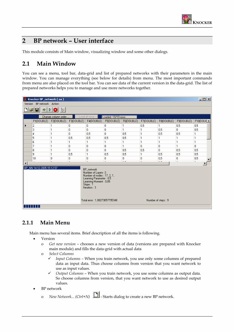
2.1 Main Window You can see a menu, tool bar, data-grid and list of prepared networks with their parameters in the main window. You can manage everything (see below for details) from menu. The most important commands from menu are also placed on the tool bar. You can see data of the current version in the data-grid. The list of prepared networks helps you to manage and use more networks together.

2.1.1 Main Menu

Main menu has several items. Brief description of all the items is following. • Version

o Get new version – chooses a new version of data (versions are prepared with Knocker main module) and fills the data-grid with actual data

o Select Columns Input Columns – When you train network, you use only some columns of prepared

data as input data. Thus choose columns from version that you want network to use as input values.

Output Columns – When you train network, you use some columns as output data. So choose columns from version, that you want network to use as desired output values.

• BP network

o New Network... (Ctrl+N) - Starts dialog to create a new BP network.


KNOCKER

o Open Network... (Ctrl+O) - Opens saved network from a special XML file. This file is in a specific format, please, use only files created by this module.

o Save Network... (Ctrl+S) - Saves created network into a special XML file. You have to specify a name and a location of the network.

o Delete – Deletes chosen network from the memory (not the file from disk!). o Update – Updates chosen network. Remember, that only certain parameters of the

network can be changed.

o Visualize network – Opens a new window with the network visualization o Error visualizing – Opens a new window with graph of global errors of the network

during the cycles. • Action

o Train (F5) - Trains the network through given data until stopping parameter is reached.

o Step Train (Shift+F5) - Trains the network through given data only by one cycle.

o Cancel Training - Stops the training of the network. o Classify... (F6) – Starts a small wizard to classify data with trained network

2.1.2 Data-Grid

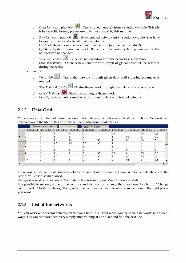
You can see current data of chosen version in the data grid. So when module starts, or choose Version> Get new version in the Menu, this grid will be filled with current data values.

There you can see values of currently selected version. Columns have got same names as in database and the type of values is also mentioned. Data-grid is read only, so you can’t edit data. If you want to, use Main Knocker module. It is possible to see only some of the columns and also you can change their positions. Use button “Change column order” to start a dialog. There, select the columns you want to see and move them to the right places you want.

2.1.3 List of the networks

You can work with several networks in the same time. It is useful when you try to train networks in different ways. You can compare them very simply after training at one place and find the best one.


KNOCKER

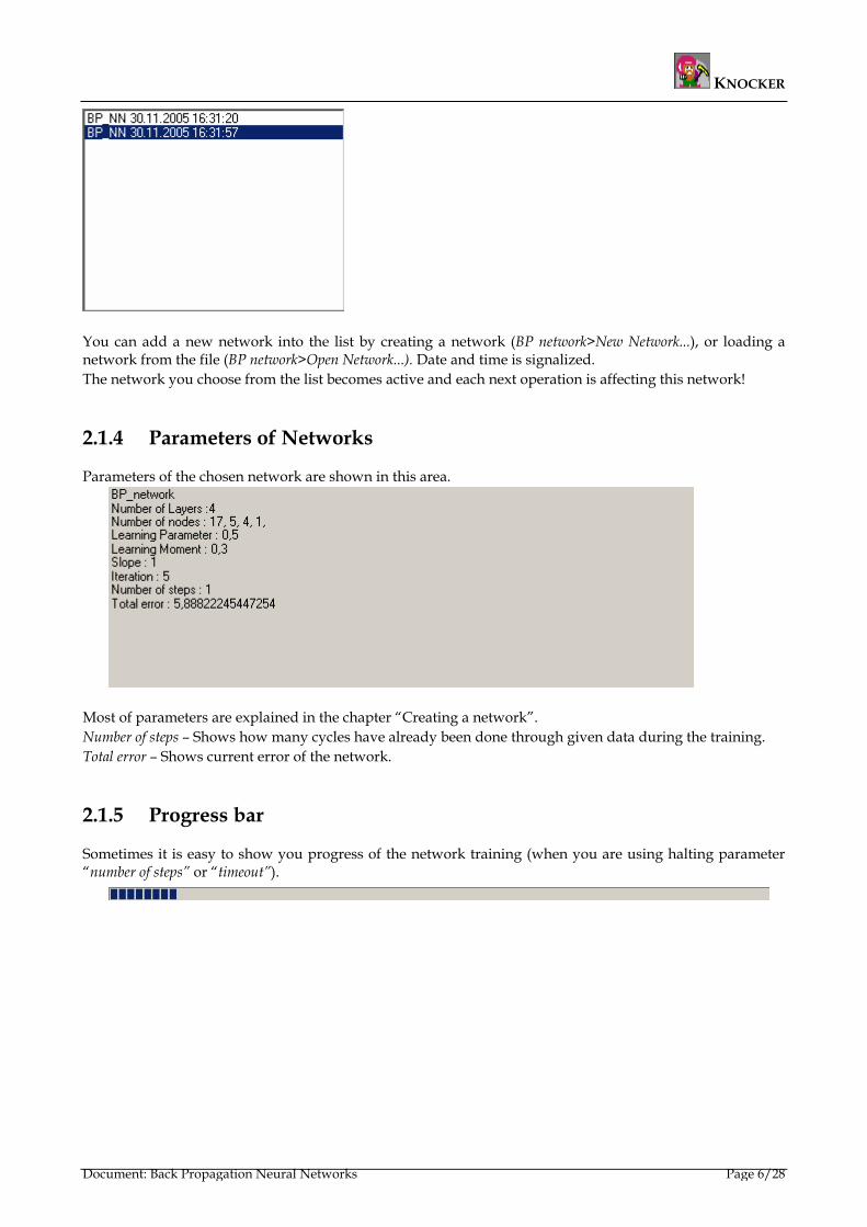
You can add a new network into the list by creating a network (BP network>New Network...), or loading a network from the file (BP network>Open Network...). Date and time is signalized. The network you choose from the list becomes active and each next operation is affecting this network!

2.1.4 Parameters of Networks

Parameters of the chosen network are shown in this area.

Most of parameters are explained in the chapter “Creating a network”. Number of steps – Shows how many cycles have already been done through given data during the training. Total error – Shows current error of the network.

2.1.5 Progress bar

Sometimes it is easy to show you progress of the network training (when you are using halting parameter “number of steps” or “timeout”).


KNOCKER

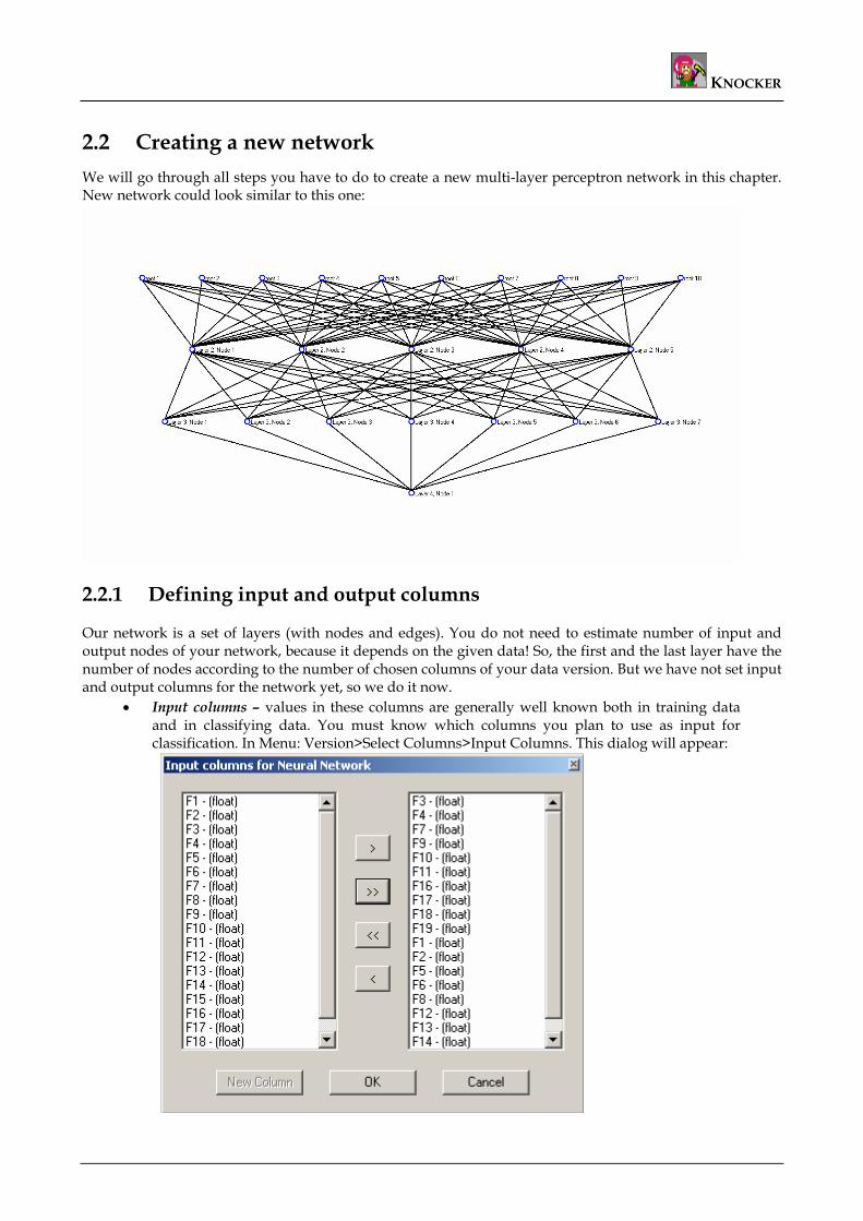
2.2 Creating a new network We will go through all steps you have to do to create a new multi-layer perceptron network in this chapter. New network could look similar to this one:

2.2.1 Defining input and output columns

Our network is a set of layers (with nodes and edges). You do not need to estimate number of input and output nodes of your network, because it depends on the given data! So, the first and the last layer have the number of nodes according to the number of chosen columns of your data version. But we have not set input and output columns for the network yet, so we do it now.

• Input columns – values in these columns are generally well known both in training data and in classifying data. You must know which columns you plan to use as input for classification. In Menu: Version>Select Columns>Input Columns. This dialog will appear:


KNOCKER

You can see all columns of the current version in the left rectangle. The right one tells you which columns will be used as input columns. Use:

- To copy one selected column from source into chosen input columns

- To copy all items from the source into chosen input columns

- To move all items from chosen input columns into the list of all columns

- To move one selected item from chosen input columns into the source When you have selected all input columns, press “OK” and your selection will be saved. When you press “Cancel”, your selection will not be saved.

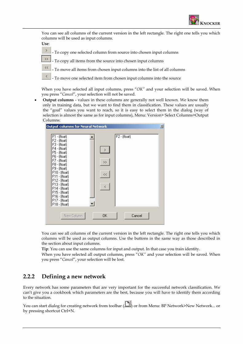
• Output columns - values in these columns are generally not well known. We know them only in training data, but we want to find them in classification. These values are usually the “goal” values you want to reach, so it is easy to select them in the dialog (way of selection is almost the same as for input columns), Menu: Version> Select Columns>Output Columns:

You can see all columns of the current version in the left rectangle. The right one tells you which columns will be used as output columns. Use the buttons in the same way as those described in the section about input columns. Tip: You can use the same columns for input and output. In that case you train identity. When you have selected all output columns, press “OK” and your selection will be saved. When you press “Cancel”, your selection will be lost.

2.2.2 Defining a new network

Every network has some parameters that are very important for the successful network classification. We can’t give you a cookbook which parameters are the best, because you will have to identify them according to the situation.

You can start dialog for creating network from toolbar ( ) or from Menu: BP Network>New Network... or by pressing shortcut Ctrl+N.


KNOCKER

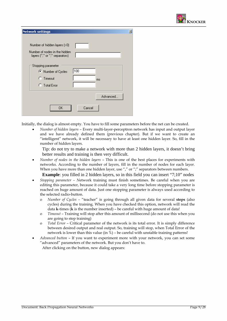
Initially, the dialog is almost empty. You have to fill some parameters before the net can be created.

• Number of hidden layers – Every multi-layer-perceptron network has input and output layer and we have already defined them (previous chapter). But if we want to create an “intelligent” network, it will be necessary to have at least one hidden layer. So, fill in the number of hidden layers. Tip: do not try to make a network with more than 2 hidden layers, it doesn’t bring better results and training is then very difficult.

• Number of nodes in the hidden layers – This is one of the best places for experiments with networks. According to the number of layers, fill in the number of nodes for each layer. When you have more than one hidden layer, use “,” or “;” separators between numbers. Example: you filled in 2 hidden layers, so in this field you can insert “7;10” nodes

• Stopping parameter – Network training must finish sometimes. Be careful when you are editing this parameter, because it could take a very long time before stopping parameter is reached on huge amount of data. Just one stopping parameter is always used according to the selected radio-button. o Number of Cycles – “teacher” is going through all given data for several steps (also

cycles) during the training. When you have checked this option, network will read the data k-times (k is the number inserted) – be careful with huge amount of data!

o Timeout – Training will stop after this amount of millisecond (do not use this when you are going to step training)

o Total Error – Critical parameter of the network is its total error. It is simply difference between desired output and real output. So, training will stop, when Total Error of the network is lower than this value (in %) – be careful with unstable training patterns!

• Advanced button – If you want to experiment more with your network, you can set some “advanced” parameters of the network. But you don’t have to.

After clicking on the button, new dialog appears:


KNOCKER

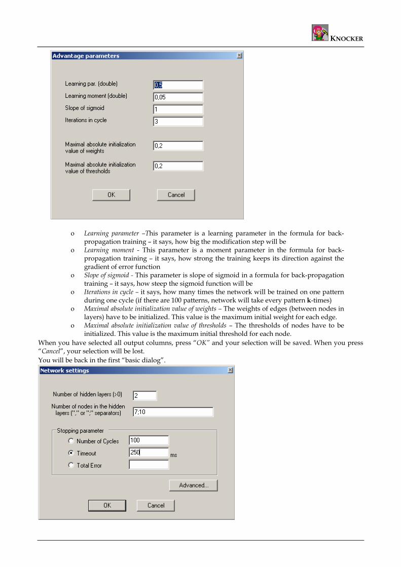
o Learning parameter –This parameter is a learning parameter in the formula for back-propagation training – it says, how big the modification step will be

o Learning moment - This parameter is a moment parameter in the formula for back-propagation training – it says, how strong the training keeps its direction against the gradient of error function

o Slope of sigmoid - This parameter is slope of sigmoid in a formula for back-propagation training – it says, how steep the sigmoid function will be

o Iterations in cycle – it says, how many times the network will be trained on one pattern during one cycle (if there are 100 patterns, network will take every pattern k-times)

o Maximal absolute initialization value of weights – The weights of edges (between nodes in layers) have to be initialized. This value is the maximum initial weight for each edge.

o Maximal absolute initialization value of thresholds – The thresholds of nodes have to be initialized. This value is the maximum initial threshold for each node.

When you have selected all output columns, press “OK” and your selection will be saved. When you press “Cancel”, your selection will be lost. You will be back in the first “basic dialog”.


KNOCKER

• OK button – program controls given parameters and creates a new BP network

After this definition, the visualization window will appear according to the created network. You can find more information about this window in a separate chapter named “Visualization”.

This window is for your information.


KNOCKER

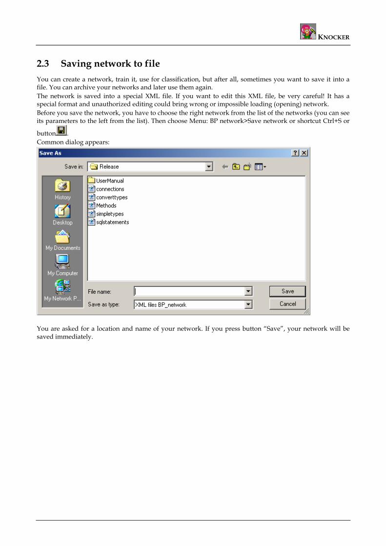
2.3 Saving network to file You can create a network, train it, use for classification, but after all, sometimes you want to save it into a file. You can archive your networks and later use them again. The network is saved into a special XML file. If you want to edit this XML file, be very careful! It has a special format and unauthorized editing could bring wrong or impossible loading (opening) network. Before you save the network, you have to choose the right network from the list of the networks (you can see its parameters to the left from the list). Then choose Menu: BP network>Save network or shortcut Ctrl+S or

button . Common dialog appears:

You are asked for a location and name of your network. If you press button “Save”, your network will be saved immediately.


KNOCKER

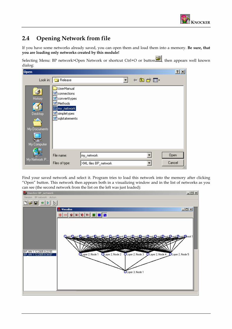
2.4 Opening Network from file If you have some networks already saved, you can open them and load them into a memory. Be sure, that you are loading only networks created by this module!

Selecting Menu: BP network>Open Network or shortcut Ctrl+O or button , then appears well known dialog:

Find your saved network and select it. Program tries to load this network into the memory after clicking “Open” button. This network then appears both in a visualizing window and in the list of networks as you can see (the second network from the list on the left was just loaded):


KNOCKER

2.5 Deleting Network from memory Every created network is saved in a memory and you can delete it. Just select it in the list of networks and choose Delete in Menu: BP network>Delete.

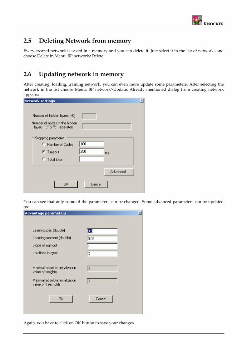
2.6 Updating network in memory After creating, loading, training network, you can even more update some parameters. After selecting the network in the list choose Menu: BP network>Update. Already mentioned dialog from creating network appears:

You can see that only some of the parameters can be changed. Some advanced parameters can be updated too:

Again, you have to click on OK button to save your changes.


KNOCKER

2.7 Visualizing network If you want to study your network, you should have idea about its structure. We have already seen a window with visualized network, but we haven’t spoken about it yet. We are going to describe the structure now.

In Menu: BP network>Visualize network or clicking on button . A special window appears.

It has two parts:

• Toolbar – helps you working with the visualized network more comfortable

o Zoom in and Zoom out the network

o Zoom in/out axis independently

o Set exact space of each node in the pixels

o Fit the tree to the window

o Fit the tree to the window always when resizing the window. Toggle button, default is pushed

• Network view – shows the structure of currently selected network. Be careful, input nodes are at the top part of the view! (Named root...). You can see input node(s), nodes of hidden layer(s) and output node(s). There are edges between them too. When you click on the edge, additional information about this node and its edges appears. Example:


KNOCKER

Selected node has a red color now. Try clicking on other nodes to see their parameters.


KNOCKER

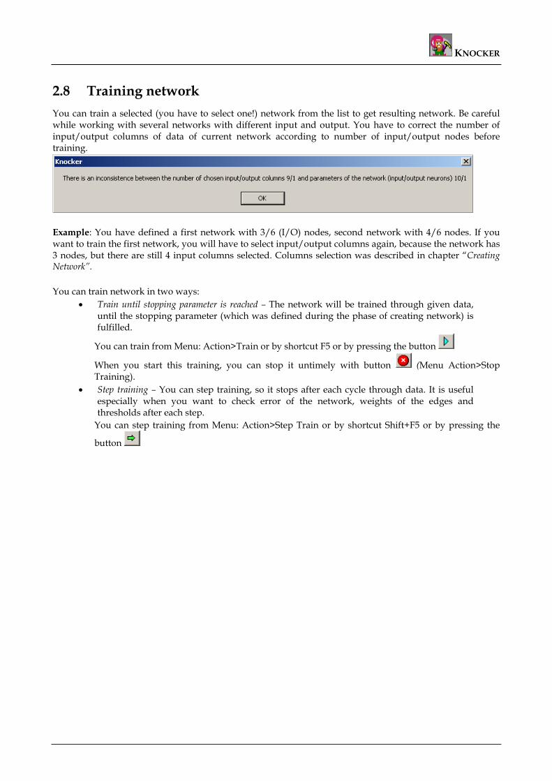
2.8 Training network You can train a selected (you have to select one!) network from the list to get resulting network. Be careful while working with several networks with different input and output. You have to correct the number of input/output columns of data of current network according to number of input/output nodes before training.

Example: You have defined a first network with 3/6 (I/O) nodes, second network with 4/6 nodes. If you want to train the first network, you will have to select input/output columns again, because the network has 3 nodes, but there are still 4 input columns selected. Columns selection was described in chapter “Creating Network”. You can train network in two ways:

• Train until stopping parameter is reached – The network will be trained through given data, until the stopping parameter (which was defined during the phase of creating network) is fulfilled.

You can train from Menu: Action>Train or by shortcut F5 or by pressing the button

When you start this training, you can stop it untimely with button (Menu Action>Stop Training).

• Step training – You can step training, so it stops after each cycle through data. It is useful especially when you want to check error of the network, weights of the edges and thresholds after each step.

You can step training from Menu: Action>Step Train or by shortcut Shift+F5 or by pressing the

button


KNOCKER

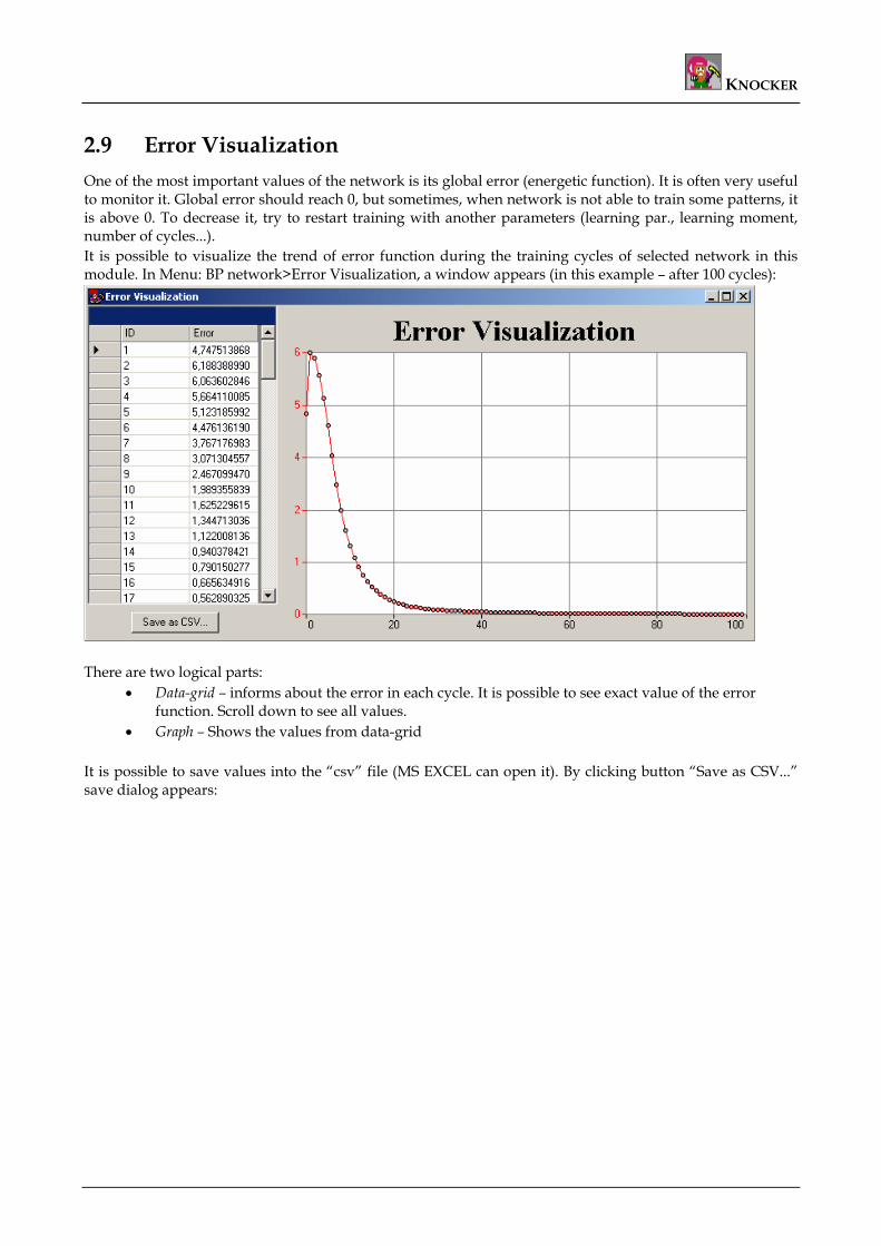
2.9 Error Visualization One of the most important values of the network is its global error (energetic function). It is often very useful to monitor it. Global error should reach 0, but sometimes, when network is not able to train some patterns, it is above 0. To decrease it, try to restart training with another parameters (learning par., learning moment, number of cycles...). It is possible to visualize the trend of error function during the training cycles of selected network in this module. In Menu: BP network>Error Visualization, a window appears (in this example – after 100 cycles):

There are two logical parts:

• Data-grid – informs about the error in each cycle. It is possible to see exact value of the error function. Scroll down to see all values.

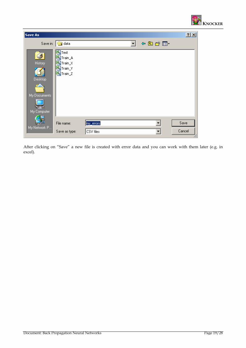
• Graph – Shows the values from data-grid It is possible to save values into the “csv” file (MS EXCEL can open it). By clicking button “Save as CSV...” save dialog appears:


KNOCKER

After clicking on “Save” a new file is created with error data and you can work with them later (e.g. in excel).


KNOCKER

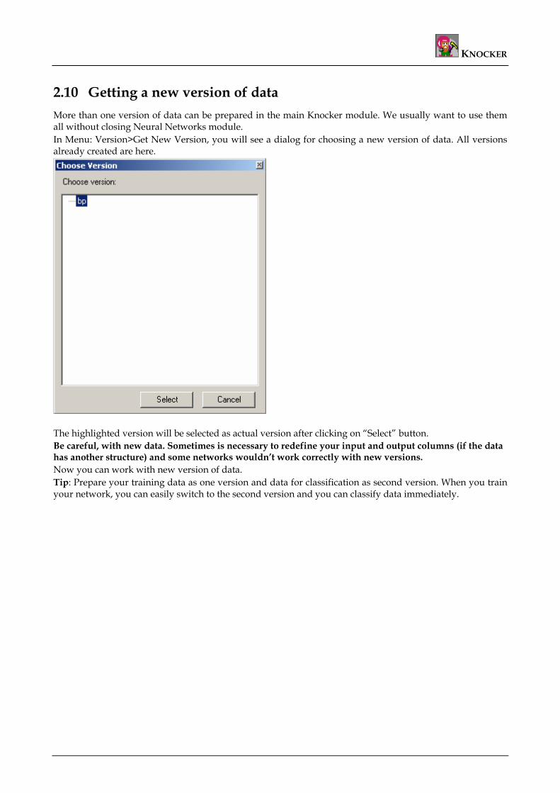
2.10 Getting a new version of data More than one version of data can be prepared in the main Knocker module. We usually want to use them all without closing Neural Networks module. In Menu: Version>Get New Version, you will see a dialog for choosing a new version of data. All versions already created are here.

The highlighted version will be selected as actual version after clicking on “Select” button. Be careful, with new data. Sometimes is necessary to redefine your input and output columns (if the data has another structure) and some networks wouldn’t work correctly with new versions. Now you can work with new version of data. Tip: Prepare your training data as one version and data for classification as second version. When you train your network, you can easily switch to the second version and you can classify data immediately.


KNOCKER

2.11 Data classification Classification is the last step and after all the work, it is like a prize. There are some steps which are necessary for successful classification:

• Trained network (the network is created or loaded and trained) • Data for classification (usually special version of data)

Classification is solved as a “wizard”. You have to go through some dialogs before your data are classified. If you press “Cancel” button, all steps will be lost. “OK” button is a gate to next dialog. In Menu: choose Action>Classify or use shortcut F6 to start classification sequence.

2.11.1 Selecting input columns

Be sure that you have selected correct columns for classification. Number of input columns should be the same as number of input nodes. This dialog was described in chapter 2.2.1

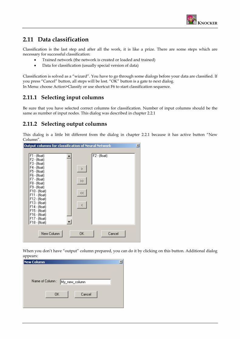
2.11.2 Selecting output columns

This dialog is a little bit different from the dialog in chapter 2.2.1 because it has active button “New Column”.

When you don’t have “output” column prepared, you can do it by clicking on this button. Additional dialog appears:


KNOCKER

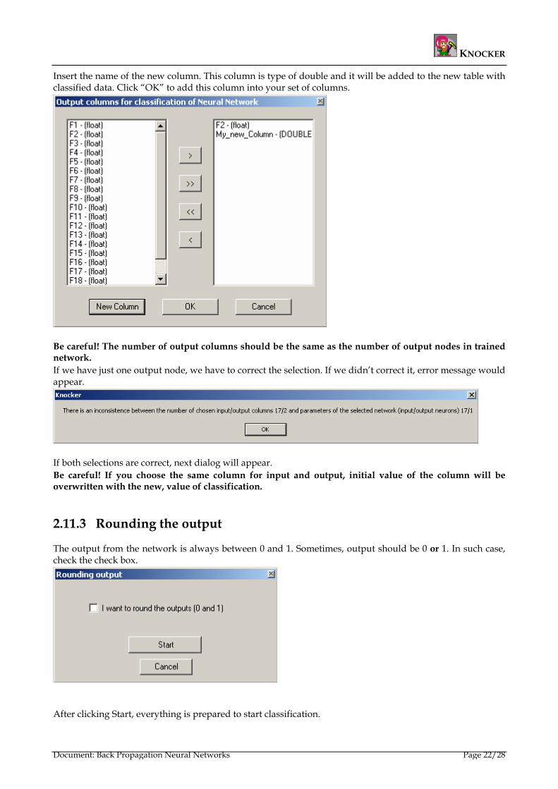
Insert the name of the new column. This column is type of double and it will be added to the new table with classified data. Click “OK” to add this column into your set of columns.

Be careful! The number of output columns should be the same as the number of output nodes in trained network. If we have just one output node, we have to correct the selection. If we didn’t correct it, error message would appear.

If both selections are correct, next dialog will appear. Be careful! If you choose the same column for input and output, initial value of the column will be overwritten with the new, value of classification.

2.11.3 Rounding the output

The output from the network is always between 0 and 1. Sometimes, output should be 0 or 1. In such case, check the check box.

After clicking Start, everything is prepared to start classification.


KNOCKER

2.11.4 Name of the new version

Classification inserts new values into the version; so new version must be created. Fill in its name. Its creation is the last step before classification.

Click “Save” and classification starts. Tip: If you want to see your new classified data then select your new version in “Menu: Version->Get New Version”:

You will see your new data in the data-grid.


KNOCKER

3 Neural Network – Tutorials There will be described one common task for back-propagation neural networks in this chapter – identity(7). We would like our network to learn all patterns – all 7-bit binary numbers (input is a 7-bit binary number and the output should be the same 7-bit binary number).

3.1 Creating a new network We have already prepared the version with data. It is available as Identity7.csv

1. Selecting input/output columns As it is described in chapter 2.2.1, choose all 7 columns as input columns and then all 7 columns as output columns.

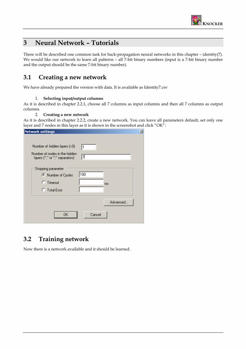
2. Creating a new network As it is described in chapter 2.2.2, create a new network. You can leave all parameters default, set only one layer and 7 nodes in this layer as it is shown in the screenshot and click “OK”:

3.2 Training network Now there is a network available and it should be learned.


KNOCKER

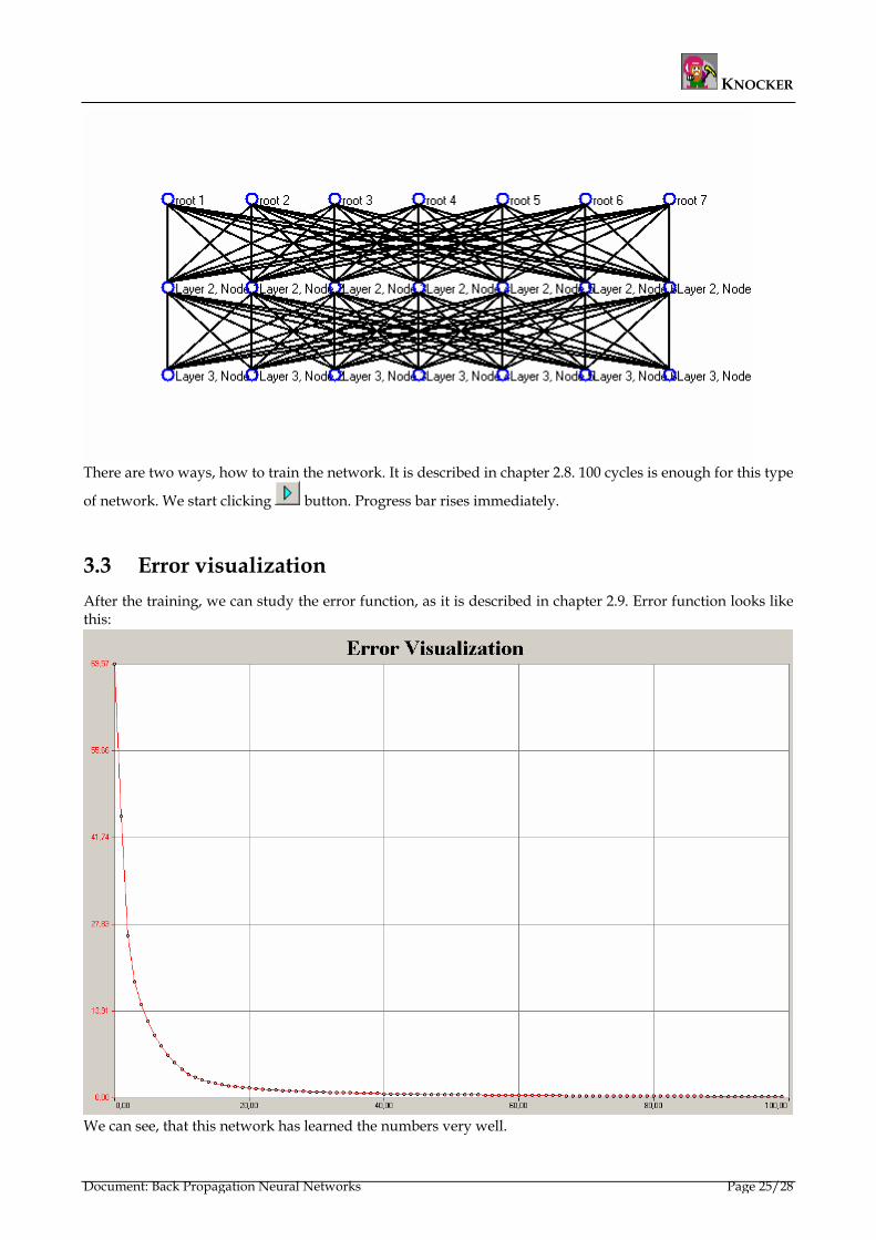
There are two ways, how to train the network. It is described in chapter 2.8. 100 cycles is enough for this type

of network. We start clicking button. Progress bar rises immediately.

3.3 Error visualization After the training, we can study the error function, as it is described in chapter 2.9. Error function looks like this:

We can see, that this network has learned the numbers very well.


KNOCKER

Tip: Try it with only 6 nodes in the hidden layer and you will see that it is impossible to train the network so well.

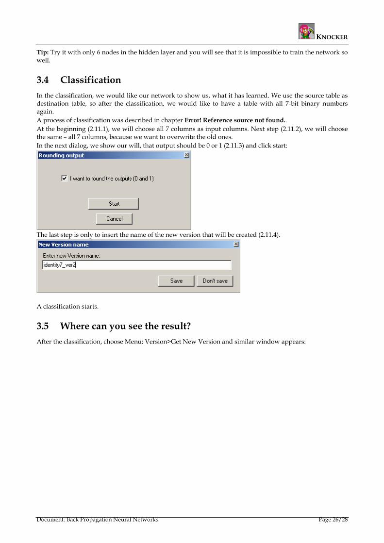
3.4 Classification In the classification, we would like our network to show us, what it has learned. We use the source table as destination table, so after the classification, we would like to have a table with all 7-bit binary numbers again. A process of classification was described in chapter Error! Reference source not found.. At the beginning (2.11.1), we will choose all 7 columns as input columns. Next step (2.11.2), we will choose the same – all 7 columns, because we want to overwrite the old ones. In the next dialog, we show our will, that output should be 0 or 1 (2.11.3) and click start:

The last step is only to insert the name of the new version that will be created (2.11.4).

A classification starts.

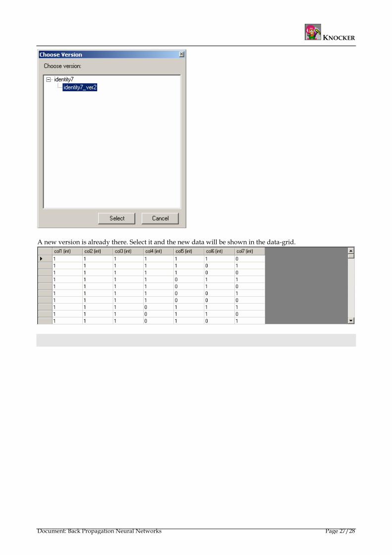
3.5 Where can you see the result? After the classification, choose Menu: Version>Get New Version and similar window appears:


KNOCKER

A new version is already there. Select it and the new data will be shown in the data-grid.


KNOCKER

4 Requirements Necessary components for correct running of this module:

• all common components of main application Knocker • BP_network.dll • DMTransformStruct.dll • PtreeViewer.dll • GuiExt.dll • Gui.dll • DasNetBarChart.dll

The main runnable class is NeuralNetStart in BP_network.dll.

5 Samples You will find some interesting sample data in CSV (Knocker friendly) format as a part of the distribution.

• identity7.csv (data from the tutorial, not-data mining, but common exercise for BP network)

• neuralnet.csv (the first column is the primary key, the second is the output) • it is possible to find large datasets in http://www.kdnuggets.com/datasets/


http://www.kdnuggets.com/datasets/

back propagation neural networks - ksvi.mff.cuni.czmraz/swprojects/knocker/user manual/back... ·...

Documents