bachelorthesis - sites.dundee.ac.uk
TRANSCRIPT

Universität der Bundeswehr München
Linda Eckel
Laboratoy Experiments of Wave Interactions on
Submerged Oscillating Bodies
Bachelorthesis
Supervisior Universität der
Bundeswehr München:
Prof. Dr. Oliver
Meyer
Supervisor University of
Dundee:
Dr. Masoud
Hayatdavoodi
14. May 2018Wehrtechnik MT 2015
Matriculation Number 1151148
Submission Date 30.09.2018

ABSTRACT
Abstract
Content of thesis is the experimental analysis of prime movers, whose �eld of ap-plication are wave enery devices in shallow water areas. These are in particularsubmerged point heaving devices with a linear generator. The basic oscillatingmotion behavior in vertical direction of di�erent forms of the prime movers undervarying conditions is investigated. The aim is to make statements about possibleoptimized forms and to suggest further test forms. Conditions are representedby di�erent submerence depths of the prime movers, as well as wave period andwave height, and by di�erent restoring forces of the connection between primemovers and linear generators. The mentioned restoring forces are simulated inthe experiments by a spring force. The horizontal position of the prime moversis �xed, the vertical movement is guided by linear bearings on a shaft. The testforms used are a circular plate and a cone whose surface shape has been adaptedto an optimized surface function of surface heaving devices with asymmetricalprime movers. Test environment is a wave �ume with piston wave maker.Furthermore, various measuring programs for determining the oscillation are pre-sented and described. These programs are able to evaluate video recordings of theexperiments with regard to the movement of the prime movers. Matlab is used asthe program interface. The presented programs are based on Gaussian Mixturemodel and color seperation. With the CamerCalibratorApp camera features areincluded.
I

DECLARATION
Declaration
I hereby declare that the work contained in this document is my own work, andthat has not been presented in a previous application for a higher degree.
Munich, 15th September 2018
II

ACKNOWLEDGEMENTS
Acknowledgements
First of all I would like to thank Dr. Hayatdavoodi for his unsel�sh support.Only because of this support, I was able to write my bachelor thesis in Scotland.Throughout the entire period, he was always available to help me and was alsoavailable to talk to me in his o�ce outside of the usual regular appointments.Through professional discussions, he was always able to open my perspective tonew aspects and motivate me anew. The experiences I gained at the University ofDundee have had a lasting impact on me and will provide me with a foundationfor my future career.
I would also like to thank the German Armed Forces. They o�ered me �nan-cial support for my student stay abroad. The participation in this project abroadhas strongly promoted my development.
III

LIST OF ABBREVIATIONS
List of Abbreviations
GMM Gaussian Mixture Model
PTO Power-take-o� system
WEC Wave Energy Converter
IV

CONTENTS
Contents
Abstract I
Declaration II
Acknowledgements III
List of Abbreviations IV
List of Figures 1
List of Tables 2
1. Introduction 3Renewable Energy . . . . . . . . . . . . . . . . . . . . . . . . . . . . . 3The Ocean as an Energy Carrier . . . . . . . . . . . . . . . . . . . . . . 4Thesis Structure . . . . . . . . . . . . . . . . . . . . . . . . . . . . . . 4
2. Literature Review 5Wave Energy Converter . . . . . . . . . . . . . . . . . . . . . . . . . . 5Current Challenges . . . . . . . . . . . . . . . . . . . . . . . . . . . . . 6Goals and Objectives . . . . . . . . . . . . . . . . . . . . . . . . . . . . 7
3. The Wave Energy Device 8
4. Experiments 10Experimental Assembly . . . . . . . . . . . . . . . . . . . . . . . . . . 10Experimental Parameters . . . . . . . . . . . . . . . . . . . . . . . . . 12
5. Design and creation of test objects with setup 14Circular Plate . . . . . . . . . . . . . . . . . . . . . . . . . . . . . . . . 14
Object Circular Plate . . . . . . . . . . . . . . . . . . . . . . . . . 14Object Cone . . . . . . . . . . . . . . . . . . . . . . . . . . . . . . . . . 14
Creation of CAD Model . . . . . . . . . . . . . . . . . . . . . . . 16Model Preparation and Calculation of Hydrodynamic Properties . 19Trouble Shooting . . . . . . . . . . . . . . . . . . . . . . . . . . . 22
6. Springs and Bearings 22Bearings . . . . . . . . . . . . . . . . . . . . . . . . . . . . . . . . . . . 22Springs . . . . . . . . . . . . . . . . . . . . . . . . . . . . . . . . . . . . 25
7. Measuring Equipment 27Wave Gauges . . . . . . . . . . . . . . . . . . . . . . . . . . . . . . . . 27Measuring Programs . . . . . . . . . . . . . . . . . . . . . . . . . . . . 27
Foreground Detector . . . . . . . . . . . . . . . . . . . . . . . . . 28Motion Tracker 2 . . . . . . . . . . . . . . . . . . . . . . . . . . . 30
8. Error Analysis 33
V

CONTENTS
9. Results and Discussion 35Analysis Testobject Circular Plate . . . . . . . . . . . . . . . . . . . . 35Analysis Testobject Cone . . . . . . . . . . . . . . . . . . . . . . . . . 42Comparison of the Test Shapes . . . . . . . . . . . . . . . . . . . . . . 43
10.Conclusion 44
Appendix 49
A. Messuring Program Foreground Detector 50
B. Messuring Program Motion Track 2 54
C. Submittal Messuring Program Motion Tracker 60
D. Basic Load Ratings Linear Bearings 63
E. Example Excerpt of Plots Erroranalysis oscillation Height 64
F. Erroranalysis Oszillation Height 65
G. Plots Oscillation Height Testobject Circular Plate 67
H. Plots Oscillation Height Testobject Cone 147
VI
LIST OF FIGURES
List of Figures
1 World Energy Demand. . . . . . . . . . . . . . . . . . . . . . . . . 32 Delimitation of Maritime Renewable Energy. . . . . . . . . . . . . 43 Types of Wave Energy Converter. . . . . . . . . . . . . . . . . . . 64 The Wave Energy Device. . . . . . . . . . . . . . . . . . . . . . . 85 Overview of experimental assembly. . . . . . . . . . . . . . . . . . 106 Wave �ume. . . . . . . . . . . . . . . . . . . . . . . . . . . . . . . 107 Particle orbits with depth. . . . . . . . . . . . . . . . . . . . . . . 118 Structure of the circular object. . . . . . . . . . . . . . . . . . . . 119 Sketch progressive wave train. . . . . . . . . . . . . . . . . . . . . 1210 Installed test object one. . . . . . . . . . . . . . . . . . . . . . . . 1411 Installed test object one on the shaft and spring. . . . . . . . . . . 1512 Asymmetric �oating energy capturer. . . . . . . . . . . . . . . . . 1613 Schematic sketch of the test object cone. . . . . . . . . . . . . . . 1614 Graphical representation of the dimensioned form function and the
approximation. . . . . . . . . . . . . . . . . . . . . . . . . . . . . 1815 Representation of the cone design. . . . . . . . . . . . . . . . . . . 1916 Sectional view of cone with dimensions. . . . . . . . . . . . . . . . 1917 Attacking forces on a stationary body in water. . . . . . . . . . . 2018 Friction coe�cient diagram. . . . . . . . . . . . . . . . . . . . . . 2519 Spring characteristics spring 1, white. . . . . . . . . . . . . . . . . 2620 Spring characteristics spring 2, red. . . . . . . . . . . . . . . . . . 2621 Erroranalysis oscillation heights of the di�erent runs as a function
of the wave height. . . . . . . . . . . . . . . . . . . . . . . . . . . 3422 Erroranalysis oscillation heights of the di�erent runs as a function
of the wave period. . . . . . . . . . . . . . . . . . . . . . . . . . . 3423 Illustration of test object platea spring one IS=0.27 P=1.75. . . . 3524 Illustration of test object plate spring one IS=0.27 P=1.00. . . . . 3625 Illustration of test object plate spring one IS=0.15 P=1.00. . . . . 3726 Illustration of the test object plate spring two. . . . . . . . . . . . 3927 Illustration of the test object cone spring two. . . . . . . . . . . . 4228 Messuring Program Foreground Detector. . . . . . . . . . . . . . . 5029 Messuring Program Motion Track 2. . . . . . . . . . . . . . . . . 5430 Submittal Messuring Program Motion Tracker. . . . . . . . . . . . 6031 Basic Load Ratings Linear Bearings[4]. . . . . . . . . . . . . . . . 63
1

LIST OF TABLES
List of Tables
1 Dimensionless experimental parameters. . . . . . . . . . . . . . . 122 Experimental parameters. . . . . . . . . . . . . . . . . . . . . . . 133 Formula symbols and values used to calculate the hydrodynamic
properties of the cone. . . . . . . . . . . . . . . . . . . . . . . . . 204 Erroranalysis, standart deviation of circular plate with spring one. 335 Analysis oszillation Height Object one. . . . . . . . . . . . . . . . 396 Analysis oszillation Height Object two. . . . . . . . . . . . . . . . 427 Erroranalysis Oszillation Height . . . . . . . . . . . . . . . . . . . 65
2
1. INTRODUCTION
1. Introduction
Renewable Energy
In this section the aspects of renewable energies are considered. Renewable en-ergy means energy from renewable resources, which are naturally replenished ona time-scale of human life or sunlight, wind, rain, tides, waves, and geothermalheat[5].
Technologies for generating energy from renewable energy sources is a majorissue in society. Due to the increasing global warming and its more visible ef-fects, a rethinking of politics and society is beginning. One goal of this new wayof thinking is to preserve the earth in such a way, that future generations canalso use this habitat. This includes stopping the emission of greenhouse gasesand creating long-term energy sources. Renewable energy sources should make asigni�cant contribution to this.
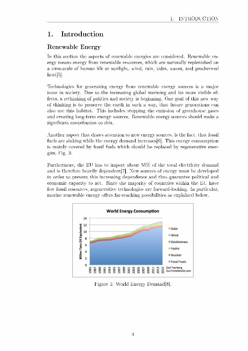
Another aspect that draws attention to new energy sources, is the fact, that fossilfuels are sinking while the energy demand increases[6]. This energy consumptionis mainly covered by fossil fuels which should be replaced by regenerative ener-gies, Fig. 9.
Furthermore, the EU has to import about 55% of the total electricity demandand is therefore heavily dependent[7]. New sources of energy must be developedin order to prevent this increasing dependence and thus guarantee political andeconomic capacity to act. Since the majority of countries within the EU havefew fossil resources, regenerative technologies are forward-looking. In particular,marine renewable energy o�ers far-reaching possibilities as explained below.
Figure 1: World Energy Demand[8].
3

1. INTRODUCTION
The Ocean as an Energy Carrier
Oceans and seas are a possible source of renewable energies. Renewable energiesproduced by using marine sources and marine space are called marine renewableenergy[7]. O�shore wind farms also belong to the category of marine renewableenergy, since by de�nition they use marine space, Fig. 2.
Due to its large energy capacity, which is many times greater than global elec-tricity demand, the ocean has an important position in the implementation ofclimate targets[9]. One of these climate targets is the reduction of CO2 to 136million tonnes[7] and many experts believe, that marine renewable energy is thebest option to reach this goal[9].However, this energy source has hardly been used to date. This is due to the var-ious challenges that projects of this kind have to overcome. The ocean and theseas are used in many di�erent ways. On the one hand through �shing, shipping,oil platforms but also through the sea inhabitants. All this must be taken intoaccount in the development of regenerative technologies.[9]
Figure 2: Delimitation of Maritime Renewable Energy[7].
Thesis Structure
This paper deals with the increasingly use of wave energy. Therefore, the follow-ing sections, are only dealing with so-called wave energy converters (WEC). Thefollowing section 4 describes and explains the model of the WEC on which thisthesis is based. This is the foundation for the test setup and the test parametersin section 4.. Then follows the design and development of the test objects andtheir components, like bearings and springs. Moving on to the analysis of the ex-perimental work, the measuring equipment and the programs for motion analysisof the test objects/prime mover are explained next. In section 8. a general erroranalysis and discussion takes place and �nally in section 9. the results and thediscussion of these.
4
2. LITERATURE REVIEW
2. Literature Review
Wave Energy Converter
WEC are systems that convert the energy, contained in waves, into other formsof energy to make them usable in form of electricity. Wave energy has the highestenergy density of all renewable resources[10]. Since this energy source has rarelybeen used so far [6], Fig. 9, wave energy o�ers many extensive possibilities. Es-pecially the coasts of Great Britain and France are large sea areas whose waveenergy can be used[10]. However, many projects are still in the R&D stage andare not yet fully developed[10]. In general, WEC are divided into four groupsaccording to their mode of function, shown in �gure 3[6].In general, WECs consist of four components. The �rst component is the foun-dation. The second the structure and the prime mover that captures the waveenergy. This captured energy is converted in a power-take-o� system (PTO) intoanother form of energy and this process is monitored by a control system.[11]
Heaving Devices
Heaving devices use the vertical oscillation of a body. This body, the primemover, can be on the surface, like a buoy, as well as underwater. The wavemovement raises and lowers the prime mover. This kinetic energy is transferredto the PTO, a linear generator. The linear generator is connected to the primemover and the sea �oor. If the prime mover goes up and down, only the rotor ismoving.[11]A linear generator corresponds to a generator whose rotor and stator have beenunwound and are moved linear to each other.
Pitching Devices
Pitching devices are semi-submerged or surface �oating cylinders. These cylindersare connected with special swivel joints, which are absorbing the wave-inducedrelative movements. The movements are absorbed by a hydraulic system anddrive the pumps. This can be used to generate electricity.[10]
Oscillating water Columns
Oscillating water columns consist of
"particular submerged hollow structures"
[10, p.16] and one or more turbines. This structure is opened under the watersurface. The wave motion causes the water within the structure to sink and rise
5

2. LITERATURE REVIEW
and causes a pressure change of the air above the water surface within the struc-ture. This changes the pressure and drives a turbine that is used to generateelectricity.[10]
Overtopping Devices
Overtopping Devices are using turbines to generate power like the oscillatingwater columns as described above. By collecting water from overturning wavesin a higher reservoir, the turbines can be driven.[10]
Figure 3: Types of Wave Energy Converter[6].
Current Challenges
Many systems are based on these four types. However, there are still many prob-lems to solve. This includes irregular wave amplitude, phase and directions whichhas an impact on e�ciency.[10]During development, operating conditions are assume. For theses conditions thesystem is designed and works e�ciently. Due to an irregular operating range, itis di�cult to de�ne the conditions and achieve high e�ciency.Furthermore, the irregular slow waves have an e�ect on the generator. The gen-erator produces a constant frequency of 50 Hz and thus 500 times higher than thefrequency of the waves, which additionally �uctuates. Despite these �uctuations,the generator must be able to generate electricity that can be fed into the powergrid. The components are also exposed to extreme weather situations and mustresist without damage.[10]
Another problem is the infrastructure and interaction with other users of themarine habitat. The existing infrastructure for power supply is designed for sys-tems whose power supply can be controlled. This is not possible with wave energy,it depends on the current environmental conditions. Therefore, electricity storagecapacities or other solutions must be created to compensate for such �uctuations.
6

2. LITERATURE REVIEW
It is also necessary for the WEC to lay supply connections on land, which meansthe construction of an underwater power grid.[12]Furthermore, the ocean is a much-used habitat. On the one hand, marine life, onthe other hand, shipping tra�c, �shermen and other consumers who should notbe in�uenced or restricted by WECs. This poses particular challenges to the de-velopment of noise for animal species and the closure of sea areas for shipping.[12]
Goals and Objectives
The content of this scienti�c work is the experimental analysis of the motion be-haviour of di�erent test objects with di�erent shapes, which are used as primemovers in a WEC. The e�ects on the motion of the prime mover by di�erentharmonic waves, submergence steps and shapes of the object, as well as di�erentsprings are investigated. The results of these tests should be used as a basis foroptimising the prime movers and give an impression of the general behaviour ofthe various test shapes in order to develop and formulate new test conditions ortest shapes.
Test parameters are wavelength, wave height, spring sti�ness, submergenstepand form of the prime mover. The water depth remains constant and is assumedto be shallow water. Five di�erent wavelengths, six wave heights, two springsand four submerged steps are tested. The tests are carried out on two test forms,a cone and a circular plate. Test environment is a wave�ume with a pistonwave-maker. In this wave�ume the test objects are mounted on a horizontal �xed shafton di�erent submergensetps. Test object and shaft are connected by a spring.The change in the spring sti�ness of this link between shaft and object is alsoincluded in the tests. Measuring systems record the movement of the waves aswell as the movement of the test objects.
7

3. THE WAVE ENERGY DEVICE
3. The Wave Energy Device
This intendet experimental analysis of the motion behavior of a prime mover hereis about the model of a WEC shown in Fig. 4. The prime mover is used later ina device, which is structured in this way or something similar. Figure 4 gives apossible impression of a constructive solution.
Figure 4: The Wave Energy Device.
The WEC presented here is a submerged heaving device. The idea and develop-ment of this WEC is originated after structual analysis. In this analysis material,wave load and the structure resbond were taken into account. The result is thedesign which is used here as well.[13]
The construction is as follows: The prime mover is located below the watersurface and is therefore submerged. As only a vertical movement of the primemover is allowed or preferred, it is a heaving device. Application area is shallowwater. In our experiments, these are water depths of 0.3 m.
As explained in chapter 2., the WEC consists of the same basic building ele-ments. A frame that is held in position by its attachment to the seabed. A primemover that absorbs and transmits the wave energy and a PTO system that gen-erates electricity from the movement of the prime mover. The prime mover canbe mounted in various submerged steps.The rectangular framework provides the necessary stability and foundation onthe seabed. The prime mover is moved vertically up and down on four guidedrails of the frame. This prevents horizontal deviation or rotation of the prime
8

3. THE WAVE ENERGY DEVICE
movers. The prime mover is connected to the PTO system. This design consistsof a linear generator, with the stator �rmly anchored and the rotor connected tothe prime mover. The Rotor shows limited possibilities of movements.In the lower area, the rotor is attached by a spring, which causes a restoringforce. In the upper area, a second spring limits the vertical de�ection by theprime mover.[14]
With the lifting and lowering movement of the prime mover, power is generatedby the linear generator. The power generation depends on the wave movementand thus the movement of the prime mover. This leads to the general problemswith WEC mentioned in section 2.. It is di�cult to control the power generation.The power P is not only dependent on the already mentioned factors of waveheight H and wave period T, but also on the wathedepth h, the shape ans thesize of the prime mover, as well as the submergence depth s, the bearing frictioncoe�cient 𝜇 and the spring sti�ness k. This is shown in equation 1.
𝑃 = 𝑓(𝐻,𝑇, ℎ, 𝑠ℎ𝑎𝑝𝑒, 𝑠𝑖𝑧𝑒, 𝑠, 𝜇, 𝑘) (1)
9

4. EXPERIMENTS
4. Experiments
Experimental Assembly
Based on the device which is presented in section 4 an experimental assemblywas developed. This is shown in �gure 5 and is explained in the following. Notethe coordinate system in this �gure, which is used continuously.
Figure 5: Overview of experimental assembly.
The experiments are carried out in a wave�ume with a 12 m long wave tank. Onthe left side of the picture, the waves are generated by a wave maker and capturedat the end of the wave tank by a wave absorber. This wave absorber, approx.1.5 m long, is designed to prevent measurement distortion caused by re�ection ofreturning waves.
Figure 6: Wave �ume.
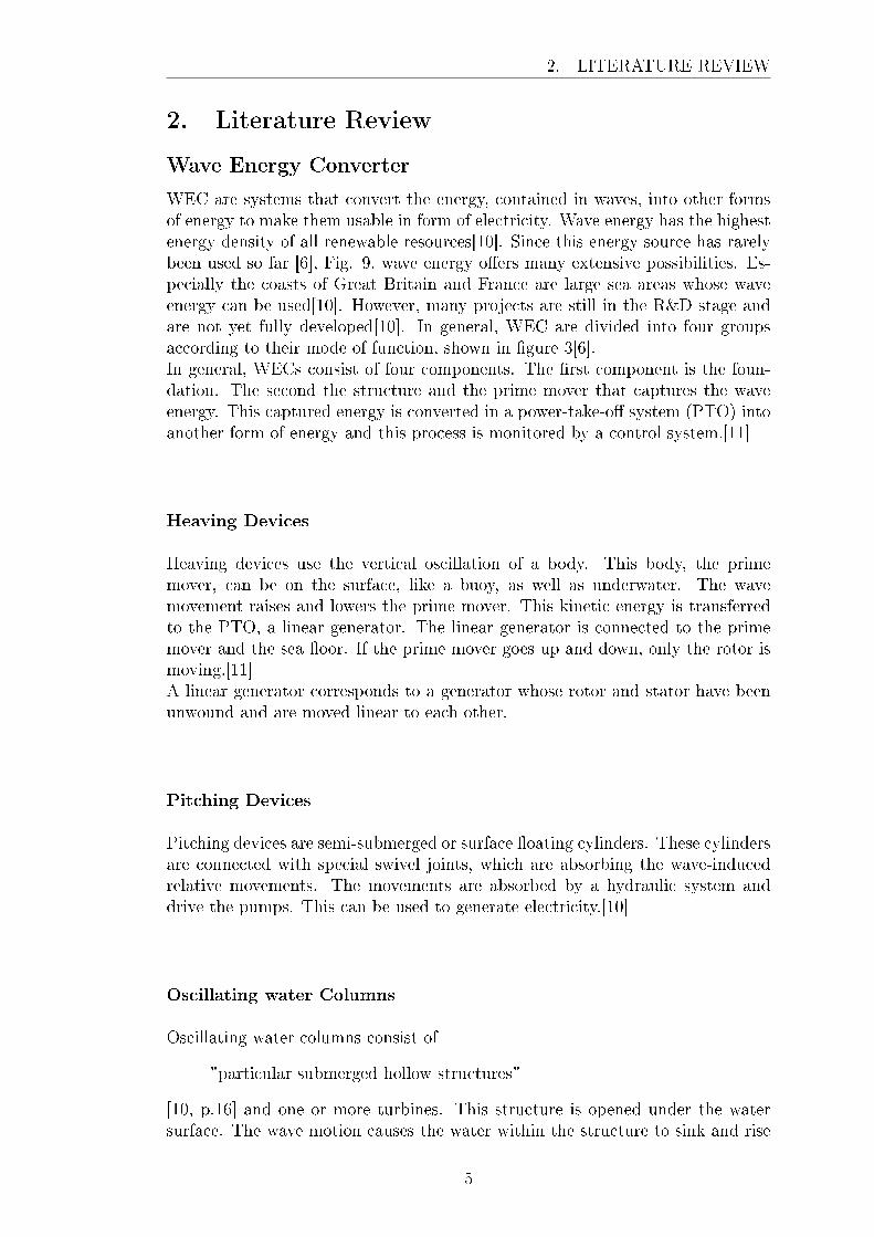
A piston wave maker is used as wave maker. This is used to simulate waves inshallow water.Generally there are three di�erent types of wave makers. Piston, �ap and plungerwave makers. The �rst two being the most common. Flap wave makers are usedfor depth water.[15]This has the background that the water particles move on an orbital. In deepwater, the orbital motion decreases and is no longer perceptible on the ground.In shallow water, the orbital trajectory becomes elliptical with increasing depth.The movement in z-direction decreases, whereas the movement in x-directionremains. This is illustrated in �gure 7.[16]The shafts are generated by three di�erent systems: pneumatic, hydraulic orelectric. The test equipment used here was operated pneumatically.[15]The movement of the wave is detected by three measuring points. Gauge one islocated at a distance of 2.1 m from the wave maker, the following two measuring
10
4. EXPERIMENTS
Figure 7: Particle orbits with depth[16].
points each have a distance of 1.5 m from the adjacent measuring point. All threegauges are mounted vertically at half the width of the wave tank.
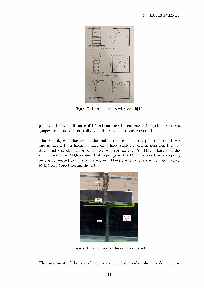
The test object is located in the middle of the measuring points one and twoand is driven by a linear bearing on a �xed shaft in vertical position, Fig. 8.Shaft and test object are connected by a spring, Fig. 8. This is based on thestructure of the PTO-system. Both springs in the PTO behave like one springon the connected driving prime mover. Therefore, only one spring is connectedto the test object during the test.
Figure 8: Structure of the circular object
The movement of the test object, a cone and a circular plate, is detected by
11
4. EXPERIMENTS
a camera which position is approximately 1.5 m away from the wave tank. Todetermine the exact camera position and angle with the position of the test object,a chessboard is used for calculation. This will later serve as a reference with thehelp of calibration images and visibility in the video recordings. The origin ofa coordinate system on the chessboard pattern, de�ned by the caliberizationimages, corresponds to a distance of 0.22 m to the bottom of the wave tank. Thisis important because the absolute movement in the shaft tank can be identi�edand not only the relative movement is known.
Experimental Parameters
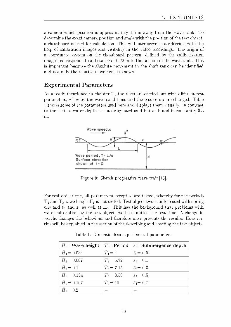
As already mentioned in chapter 2., the tests are carried out with di�erent testparameters, whereby the wave conditions and the test setup are changed. Table1 shows some of the parameters used here and displays them visually. In contrastto the sketch, water depth is not designated as d but as h and is constantly 0.3m.
Figure 9: Sketch progressive wave train[16].
For test object one, all parameters except s0 are tested, whereby for the periodsT4 and T5 wave height H1 is not tested. Test object two is only tested with springone and s0 and s1 as well as H6. This has the background that problems withwater adsorption by the test object two has limitted the test time. A change inweight changes the behaviour and therefore misrepresents the results. However,this will be explained in the section of the describing and creating the test objects.
Table 1: Dimensionless experimental parameters.
�̄�= Wave height 𝑇= Period 𝑠= Submergence depth
�̄�1= 0.034 𝑇 1= 4 𝑠0= 0.0
�̄�2= 0.067 𝑇 2= 5.72 𝑠1= 0.1
�̄�3= 0.1 𝑇 3= 7.15 𝑠2= 0.3
�̄�4= 0.134 𝑇 4= 8.58 𝑠3= 0.5
�̄�5= 0.167 𝑇 5= 10 𝑠4= 0.7
�̄�6= 0.2 − −
12

4. EXPERIMENTS
In the next step, these parameters are referred to the water depth h which is usedin the experiments, Eqs. (2) to (4).
𝑇 =𝑇√︀
𝑔ℎ
(2)
�̄� =𝐻
ℎ(3)
𝑠 = 𝑠/ℎ (4)
This results in the following test parameters shown in table 2.
Table 2: Experimental parameters.
H= Waveheight [m]
T= Period [s] s= Submer-gence depth[m]
IS= Inertialsubmergencedepth [m]
H1= 0.01 T1= 0.70 s0= 0.00 IS0= 0.30
H2= 0.02 T2= 1.00 s1= 0.03 IS1= 0.27
H3= 0.03 T3= 1.25 s2= 0.09 IS2= 0.21
H4= 0.04 T4= 1.50 s3= 0.15 IS3= 0.15
H5= 0.05 T5= 1.75 s4= 0.21 IS4= 0.09
H6= 0.06 − − −
Due to the higher accuracy of the positioning of the test objects, the position ofthe objects is shown below as IS as the distance from the tank bottom to theupper edge of the test objects. This is expressed by equation (5).
𝐼𝑆 = ℎ− 𝑠 (5)
All parameters are combined in a way that both test objects are tested with twodi�erent springs. The test objects are tested for all theire wave conditions, i.e.period and wave height, which were explained before.
The water density 𝜌 is constant during the experiments and is 997 kg/m3.
13
5. DESIGN AND CREATION OF TEST OBJECTS WITH SETUP
5. Design and creation of test objects with setup
Circular Plate
Object Circular Plate
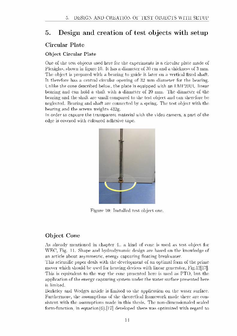
One of the test objects used here for the experiments is a circular plate made ofPlexiglas, shown in �gure 10. It has a diameter of 30 cm and a thickness of 3 mm.The object is prepared with a bearing to guide it later on a vertical �xed shaft.It therefore has a central circular opening of 32 mm diameter for the bearing.Unlike the cone described below, the plate is equipped with an LMF20UU linearbearing and can hold a shaft with a diameter of 20 mm. The diameter of thebearing and the shaft are small compared to the test object and can therefore beneglected. Bearing and shaft are connected by a spring. The test object with thebearing and the screws weights 432g.In order to capture the transparent material with the video camera, a part of theedge is covered with coloured adhesive tape.
Figure 10: Installed test object one.
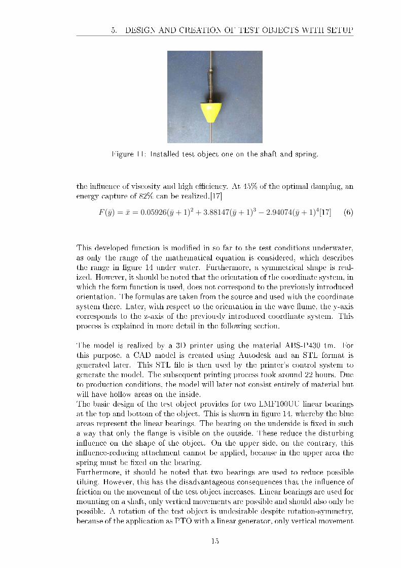
Object Cone
As already mentioned in chapter 4., a kind of cone is used as test object forWEC, Fig. 11. Shape and hydrodynamic design are based on the knowledge ofan article about asymmetric, energy-capturing �oating breakwater.This scienti�c paper deals with the development of an optimal form of the primemover which should be used for heaving devices with linear generator, Fig.12[17].This is equivalent to the way the cone presented here is used as PTO, but theapplication of the energy capturing system under the water surface presented hereis limited.Berkeley and Wedges article is limited to the application on the water surface.Furthermore, the assumptions of the theoretical framework made there are con-sistent with the assumptions made in this thesis. The non-dimensionaled scaledform-function, in equation(6),[17] developed there was optimized with regard to
14
5. DESIGN AND CREATION OF TEST OBJECTS WITH SETUP
Figure 11: Installed test object one on the shaft and spring.
the in�uence of viscosity and high e�ciency. At 45% of the optimal damping, anenergy capture of 82% can be realized.[17]
𝐹 (𝑦) = �̄� = 0.05926(𝑦 + 1)2 + 3.88147(𝑦 + 1)3 − 2.94074(𝑦 + 1)4[17] (6)
This developed function is modi�ed in so far to the test conditions underwater,as only the range of the mathematical equation is considered, which describesthe range in �gure 14 under water. Furthermore, a symmetrical shape is real-ized. However, it should be noted that the orientation of the coordinate system, inwhich the form function is used, does not correspond to the previously introducedorientation. The formulas are taken from the source and used with the coordinatesystem there. Later, with respect to the orientation in the wave �ume, the y-axiscorresponds to the z-axis of the previously introduced coordinate system. Thisprocess is explained in more detail in the following section.
The model is realized by a 3D printer using the material ABS-P430 tm. Forthis purpose, a CAD model is created using Autodesk and an STL format isgenerated later. This STL �le is then used by the printer's control system togenerate the model. The subsequent printing process took around 22 hours. Dueto production conditions, the model will later not consist entirely of material butwill have hollow areas on the inside.The basic design of the test object provides for two LMF100UU linear bearingsat the top and bottom of the object. This is shown in �gure 14, whereby the blueareas represent the linear bearings. The bearing on the underside is �xed in sucha way that only the �ange is visible on the outside. These reduce the disturbingin�uence on the shape of the object. On the upper side, on the contrary, thisin�uence-reducing attachment cannot be applied, because in the upper area thespring must be �xed on the bearing.Furthermore, it should be noted that two bearings are used to reduce possibletilting. However, this has the disadvantageous consequences that the in�uence offriction on the movement of the test object increases. Linear bearings are used formounting on a shaft, only vertical movements are possible and should also only bepossible. A rotation of the test object is undesirable despite rotation-symmetry,because of the application as PTO with a linear generator, only vertical movement
15

5. DESIGN AND CREATION OF TEST OBJECTS WITH SETUP
Figure 12: Asymmetric �oating energy capturer. Based on [17].
can be changed into electrical energy.Also the in�uence of the movement at the shaft should be kept as small as possible.In relation to the expected size of the test object, a shaft with a diameter of 10mm is selected. This diameter is small compared to the �nal test object andhas no signi�cant in�uence on the experiments. The selection of shaft diameterstherefore also justi�es the selection of bearings.
Figure 13: Schematic sketch of the test object cone.
Creation of CAD Model
To create the CAD model with the geometric data, the function mentioned inthe previous section had to be incorporated �rst.In the �rst step, the non-dimensional form function is related to the dimensionsof the later model. The dimensions of the cone are limited by the maximumcomponent size of the printer and the wave tank. The available 3D printer has aproduction space of 6x8x6 inches. This corresponds to about 150x200x150 mm.During the experiments with a water depth of 300 mm and various submergencesteps, the cone should not be larger than 15 cm in height, taking the oscillationof the object into account. The width of the object is determined by the produc-tion dimensions of the printer, because the tank is considerably wider than the
16

5. DESIGN AND CREATION OF TEST OBJECTS WITH SETUP
production possibilities allow. The cone should be 15x15x15 cm. For y<0 thefollowing equations (7) and (8) can be used. Where b and D represent the radiusb of the cone and the height D as shown in �gure 12.
�̄� = 𝑥/𝑏 (7)
𝑦 = 𝑦/𝐷 (8)
However, it should be noted that D de�nes the height from x=b to x=0. Thecoordinate system is located in the rotation axis of the cone. If x is zero, ataper with a pointed tip is formed. However, as already described and shown inthe sketch, a bearing should be �tted to the lower end of the cone and a shaftshould pass through this bearing. The test object should therefore be a truncatedcone. Therefore, in our application case, x will not be zero. The diameter of the�ange of the bearing, which should rest on the lower end of the cone, is 40 mm.Therefore the lower diameter of the blunt cone should be about 41 mm and thusthe radius 20.5 mm de�ned as rF. This de�nes the range of the form functiontaking into account the still valid assumption 𝑦 < 0 as follows:
[−𝑏,−𝑟𝐹 ) = [−𝑏,−𝑟𝐹 [:= {𝑥 ∈ R | −𝑏 ≤ 𝑥 < −𝑟𝐹} (9)
(𝑟𝐹 , 𝑏] =]𝑟𝐹 , 𝑏] := {𝑥 ∈ R | 𝑟𝐹 < 𝑥 ≤ 𝑏} (10)
As already mentioned, D describes the height of the cone from x=b to x=0.Due to the changed interval, the cone will later have the height D* and not D.Therefore, |D*| = 23 cm and |b| = 7 cm were selected as untagging parameters.The dimensioned function is expressed by equation (11).
𝐹 (𝑦) = 𝑥 =𝑏
𝐷* [0.05926(𝑦 +
1
𝐷)2 + 3.88147(𝑦 +
1
𝐷)3 − 2.94074(𝑦 +
1
𝐷)4] (11)
In the next step of creation, a table was designed. Starting from 0, the y valueincreases in 0.05 steps to y=23. With the de�ned increment for y and the heightD the corresponding 𝑦 values are calculated with formula (8) and inserted intothe function (6). With the �̄� values assigned from this and the previously de�nedradius b, the dimensioned x values are calculated from equation (7). With thesey and x values a 6th-order approximated function (12) was designed.
The creation of the table has the background of a visual examination of thecone shape as well as modelling reasons. The form function must be integratedinto CAD to generate the conical model. There are two ways to do this in the
17

5. DESIGN AND CREATION OF TEST OBJECTS WITH SETUP
software which was used. On the one hand, functions can be modeled by coor-dinate points, on the other hand, curves can be speci�ed as functions by F(x).Since the �rst option only displays the shape without including the shape curve inthe creation of the model, the second option is used. However, the form function(6) which is used in literature is a function F(y). Instead of a complex mathe-matical calculation operation to adapt the function to the software requirements,the table values of the visual inspection are used to create an approximate curve.This approximation, equation 12, is a 6th-order function depending on x and thedomain of equation (9). This method meets the accuracy requirements, since themanufacturing tolerances are greater than the deviations from 0.6mm resultingfrom the approximation.
𝐹 (𝑥) = 0, 0112𝑥6+0, 2888𝑥5+3, 0133𝑥4+16, 274𝑥3+47, 788𝑥2+70, 088𝑥+27, 427(12)
Figure 14: Graphical representation of the dimensioned form function and theapproximation.
After modelling the outer shape of the cone, the wall thicknesses are modelled.Due to production reasons, the test object cannot consist entirely of material.The wall thicknesses were chosen in such a way, that there is at each point a min-imum material thickness of 11.4 mm. This thickness is su�cient to attach thebearings with the help of screws without drilling through the walls and getting
18
5. DESIGN AND CREATION OF TEST OBJECTS WITH SETUP
into the interior. Drilling through the hole poses a risk of water ingress.
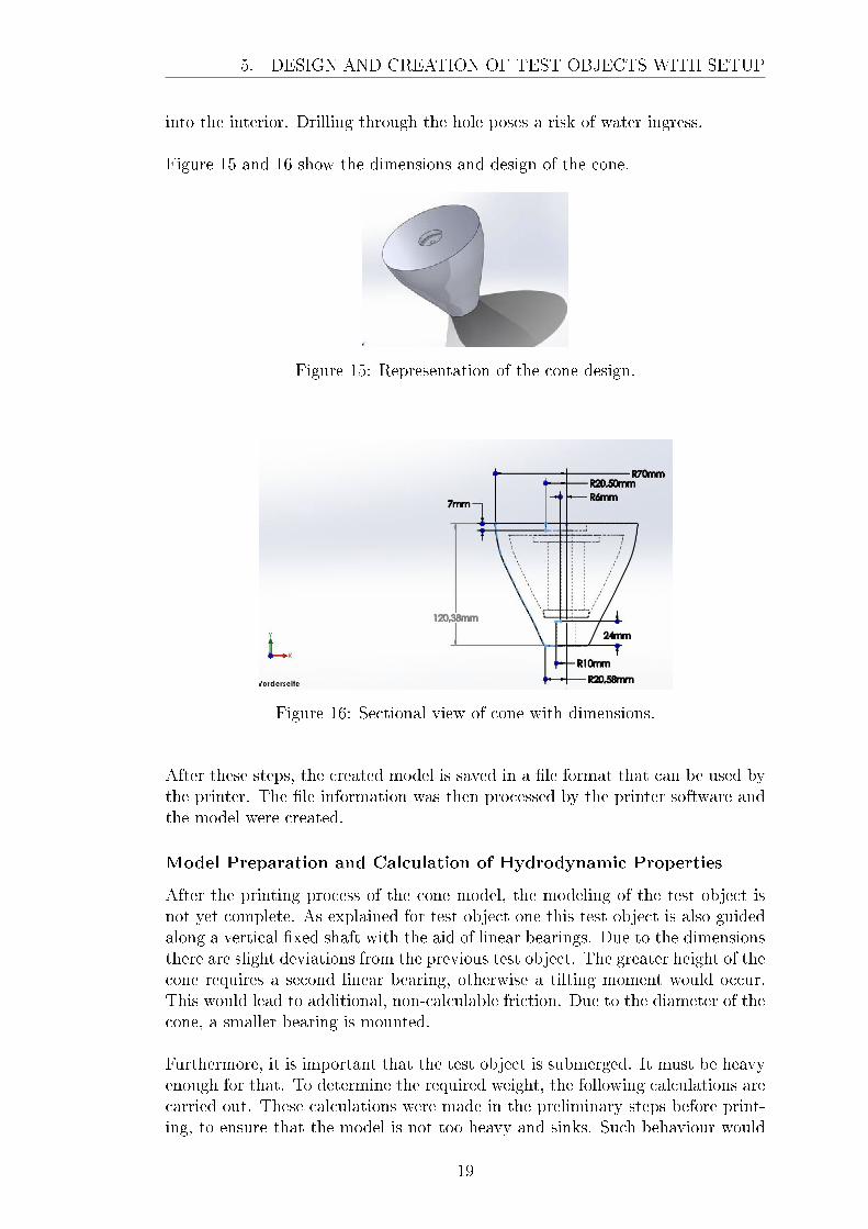
Figure 15 and 16 show the dimensions and design of the cone.
Figure 15: Representation of the cone design.
Figure 16: Sectional view of cone with dimensions.
After these steps, the created model is saved in a �le format that can be used bythe printer. The �le information was then processed by the printer software andthe model were created.
Model Preparation and Calculation of Hydrodynamic Properties
After the printing process of the cone model, the modeling of the test object isnot yet complete. As explained for test object one this test object is also guidedalong a vertical �xed shaft with the aid of linear bearings. Due to the dimensionsthere are slight deviations from the previous test object. The greater height of thecone requires a second linear bearing, otherwise a tilting moment would occur.This would lead to additional, non-calculable friction. Due to the diameter of thecone, a smaller bearing is mounted.
Furthermore, it is important that the test object is submerged. It must be heavyenough for that. To determine the required weight, the following calculations arecarried out. These calculations were made in the preliminary steps before print-ing, to ensure that the model is not too heavy and sinks. Such behaviour would
19
5. DESIGN AND CREATION OF TEST OBJECTS WITH SETUP
prevent oscillation by the waves and is therefore an obstacle to the intended use.
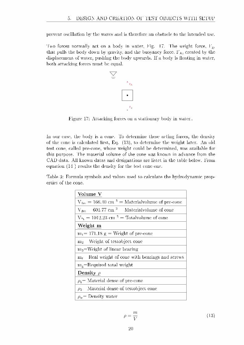
Two forces normally act on a body in water, Fig. 17. The weight force, Fg,that pulls the body down by gravity, and the buoyancy force, FA, created by thedisplacement of water, pushing the body upwards. If a body is �oating in water,both attacking forces must be equal.
Figure 17: Attacking forces on a stationary body in water..
In our case, the body is a cone. To determine these acting forces, the densityof the cone is calculated �rst, Eq. (13), to determine the weight later. An oldtest cone, called pre-cone, whose weight could be determined, was available forthis purpose. The material volume of the cone was known in advance from theCAD data. All known datas and designations are listet in the table below. Fromequation (14 ) results the density for the test cone one.
Table 3: Formula symbols and values used to calculate the hydrodynamic prop-erties of the cone.
Volume V
V1m = 166.40 cm 3 = Materialvolume of pre-cone
V2m = 601.77 cm 3 = Materialvolume of cone
V2t = 1012.23 cm 3 = Totalvolume of cone
Weight m
m1= 171.18 g = Weight of pre-cone
m2= Weight of testobject cone
m3=Weight of linear bearing
mr= Real weight of cone with bearings and screws
mg=Required total weight
Density 𝜌
𝜌1= Material dense of pre-cone
𝜌2= Material dense of testobject cone
𝜌w= Density water
𝜌 =𝑚
𝑉(13)
20

5. DESIGN AND CREATION OF TEST OBJECTS WITH SETUP
𝜌1 =𝑚1
𝑉1𝑚=
=0.1712𝑘𝑔
166.4 * 10−6𝑚3= 1028
𝑘𝑔
𝑚3(14)
Since cone one and the test object cone two, consist of the same material, thecondition (15) is assumed.
𝜌1 = 𝜌2 (15)
By converting equation (13) to equation (16) and inserting the values of conetwo, the mass of the test object can now be calculated.
𝑚 = 𝜌 * 𝑉 (16)
𝑚2 = 𝜌1 * 𝑉2𝑚 = 1028𝑘𝑔
𝑚3* 601.77 * 10−6𝑚3 = 0.6186𝑘𝑔 = 618.6𝑔 (17)
As previously mentioned, the test object should not sink nor swim. In the idealcase, the body should �oat or sink very slightly. Thus the following force relationresults from equation (18).
𝐹𝐴 = 𝐹𝑔 (18)
The weight force FG results from the following components:
𝐹𝑔 = 𝑚 * 𝑔 (19)
Because this equation takes the total mass of the test object into account, theweight of both bearings must be taken recognized in the calculation:
𝐹𝑔 = (𝑚2 + 2𝑚3) * 𝑔 = (2 * 0.062𝑘𝑔 + 0.6182𝑘𝑔) * 9.81𝑚
𝑠2= 6.1𝑁 (20)
The buoyancy force is described by equation 21. Decisive for the force is not, as inequation (14) and (17), the volume of the areas which are consisting of material,but the displacement volume of the cone. The Archimedean principle states thatthe buoyancy force of the test object in the medium is equal to the weight force ofthe medium, which is displaced by the object. The volume created by the shapeof the object is displaced by the cone. Described here as V2t and taken from theCAD data.
𝐹𝐴 = 𝑉 * 𝑔 * 𝜌𝑤 (21)
𝐹𝐴 = 𝑉2𝑡 * 𝑔 * 𝜌𝑤 = 1.012 * 10−6𝑚3 * 9.81𝑚
𝑠2* 997
𝑘𝑔
𝑚3= 9.9𝑁 (22)
This proves, that the buoyancy force is signi�cantly greater than the weight force.Therefore, additional weight must be applied. This is calculated in the followingin which the weight force is required as in condition (18). This is set equal tothe buoyancy force and equation (19) is replaced to equation (23). This resultsin the missing mass of 353g.
𝑚𝑔 =𝐹𝐴
𝑔(23)
21

6. SPRINGS AND BEARINGS
𝑚𝑔 =𝐹𝐴
𝑔=
9.9𝑁
9.81𝑚𝑠2
= 1𝑘𝑔 (24)
𝑚𝑎 = 𝑚𝑔 −𝑚𝑟 = 1000𝑔 − 647𝑔 = 353𝑔 (25)
Trouble Shooting
After creating a �rst test object of the cone, another test object had to be createddue to incorrect dimensions. The reason for this was an automatically activatedoption in the CAD program, which increases all dimensions by a factor. However,this was determined after the object was printed. This faulty cone is the pre-conedescribed above and the basis for the hydrodynamic calculation.After the completion of a new test and the assembly of the other components,the �rst test runs were started. However, it turned out that the material whichwas used for the cone has an absorbing e�ect in the water. For this reason, theconnection to the bearing was painted and sealed with silicone. This led to aslight change in surface and weight. Furthermore, the additional mass ma was357g. Therefore the weight of the cone was recorded again with mg= 1033g.The measures applied also led to a positive change, but the design solution forthe arrangement of the bearings is inadequate. Both bearings must be arrangedvery precisely on a straight line, which is di�cult to achieve due to the typeof assembly and the inaccuracy of the screw holes. This leads to considerablefriction and distorts the measurement data.Therefore the lower bearing was removed and the experiments were carried outwith only one bearing. This causes additionally water absorption by separatingthe components, as well as tilting of the shaft in the bearing. The real mass usedexperimentally is therefore 971g. Since the duration of the experiments is shortand the absorbed mass is small compared to the mass of the test object, the masschange is acceptable.
6. Springs and Bearings
In this section the friction, caused by the bearings, and the determination of thespring sti�ness are explained in more detail. These are attached to the test objectas already explained in the experimental assembly.
Bearings
The bearing friction is caused by horizontal forces acting in the direction of theshaft center of the vertical test arrangement. These forces are generated by thewaves in the wave �ume. If the forces, which are acting on the bearing in thehorizontal direction, are known, the bearing friction can be calculated with theaid of the manufacturer's speci�cations.
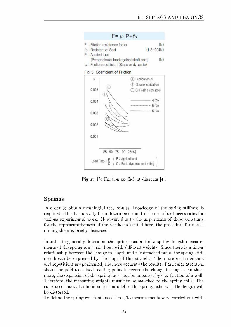
This is illustrated in �gure 18. The diagram shows a manufacturer-de�ned de-pendence between the friction constant 𝜇 and the force P acting "against shaftcore"[4] direction. The forces causing friction in the bearing are rated at size C,
22

6. SPRINGS AND BEARINGS
dynamic basic load, with reference to the size and type of bearing, see appendixD.. These values are manufacturer's speci�cations and are C1= 860 N for thebearing of the circular plate and C2= 370 N for the bearing of the cone.[4]
In the �rst step of friction determination, the force which is induced by thewaves in the x-direction is therefore calculated. According to the manufacturer,a change of the bearing friction with the force only occurs for a P/C ratio over20%. Therefore an assumption is made. Due to the high basic load rating values,considerable forces must be generated by the waves in the wave �ume. Accordingto initial estimates, however, this is not the case. Therefore, the forces for thecondition of a �xed test object and thus �xed bearings are calculated. The forcesacting on this assumption are greater than on an oscillating object.Equation (26) describes the horizontally acting force Fx, which acts on a �xedbody with the length LD at a wave height H and period T and immersion depthsd. All parameters used are dimensionless, marked by a crossbar.
𝐹𝑥 = 3.60 * �̄�2 * 𝑠𝑑0.11 * (1 − 𝑒0.09*𝑇 )(1 − 𝑒−�̄�𝐷)[18] (26)
For wave height and wave period the already dimensionless calculated values fromsection 4. are used. Since the largest e�ective force Fx is generated at the watersurface by the greatest wave height and wave period, the values of H1 and P1 areused. Where index 1 corresponds to the force of the test object plate and index2 corresponds to the cone.Furthermore, this nomenclature refers the submergence depth sd in relation tothe see�oor, i.e. our tank �oor. This corresponds to the inertial submergencedepth IS1 from chapter 4., but IS is not standardized and must therefore still berelated to the water depth, Eq. (27). Also the length LD of the test objects mustbe standardized in relation to the water depth, Eqs. (28,29). Here LD1 representslength of the test object circular plate and LD2 represents length of the cone.
𝑠𝑑 =𝐼𝑆1
ℎ=
0.27𝑚
0.3𝑚= 0.767[18] (27)
�̄�𝐷1 =𝐿𝐷1
ℎ=
0.3𝑚
0.3𝑚= 1[18] (28)
�̄�𝐷2 =𝐿𝐷2
ℎ=
0.14𝑚
0.3𝑚= 0.47[18] (29)
After this normalisation, the forces, acting on the test objects, can be calculatedand are then dimensioned to our experimental setup using equation (30) to (34).For this the length BD of the test objects, perpendicular to the shaft direction,is required. Since both test objects are circular, this length corresponds to thelength LD. The height of the test object tB corresponds to 1 tB1=0.003m for thetest object cone tB2=0.124m.
𝐹𝑥 = 𝐹𝑥 * 𝜌 * 𝑔 * ℎ * 𝑡𝐵 *𝐵𝐷[18] (30)
¯𝐹𝑥,1 = 3.60 * 0.22 * 0.7670.11 * (1 − 𝑒0.09*10)(1 − 𝑒−1) = −0.1313 (31)
23

6. SPRINGS AND BEARINGS
𝐹𝑥,1 = 𝐹𝑥,1*𝜌*𝑔*ℎ*𝑡𝐵*𝐵𝐷 = −0.1313*997𝑘𝑔/𝑚3*𝑔*0.3𝑚*0.003𝑚*0.3𝑚 = 0.35𝑁(32)
¯𝐹𝑥,2 = 3.60 * 0.22 * 0.7670.11 * (1 − 𝑒0.09*10)(1 − 𝑒−0.47) = −0.078 (33)
𝐹𝑥,2 = 𝐹𝑥,2*𝜌*𝑔*ℎ*𝑡𝐵 *𝐵𝐷 = −0.78*997𝑘𝑔/𝑚3*𝑔*0.3𝑚*0.124𝑚*0.3𝑚 = 8.5𝑁(34)
After calculating the forces, these are set in relation to the dynamic basic loadratings. The ratio calculated from this, equation (35) and (36), is used to deter-mine the coe�cient of friction for the two di�erent bearing types from equation(32) and (34). From the Graph, Fig. 18, the function two is used to taking lubri-cation losses caused by the release of grease by water into account. This resultsin a bearing friction of 𝜇=0.0048 for both test objects.
𝐹𝑥,1
𝐶1
=0.33𝑁
860𝑁= 0.41% (35)
𝐹𝑥,2
𝐶2
=8.5𝑁
370𝑁= 2.3% (36)
24
6. SPRINGS AND BEARINGS
Figure 18: Friction coe�cient diagram [4].
Springs
In order to obtain meaningful test results, knowledge of the spring sti�ness isrequired. This has already been determined due to the use of test accessories forvarious experimental work. However, due to the importance of these constantsfor the representativeness of the results presented here, the procedure for deter-mining them is brie�y discussed.
In order to generally determine the spring constant of a spring, length measure-ments of the spring are carried out with di�erent weights. Since there is a linearrelationship between the change in length and the attached mass, the spring sti�-ness k can be expressed by the slope of this straight. The more measurementsand repetitions are performed, the more accurate the results. Particular attentionshould be paid to a �xed reading point to record the change in length. Further-more, the expansion of the spring must not be impaired by e.g. friction of a wall.Therefore, the measuring weights must not be attached to the spring coils. Theruler used must also be mounted parallel to the spring, otherwise the length willbe distorted.To de�ne the spring constants used here, 13 measurements were carried out with
25
6. SPRINGS AND BEARINGS
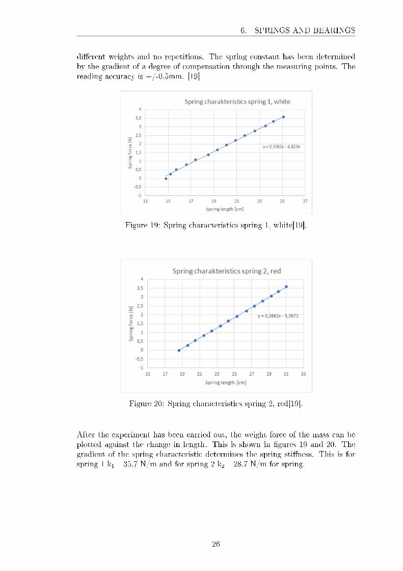
di�erent weights and no repetitions. The spring constant has been determinedby the gradient of a degree of compensation through the measuring points. Thereading accuracy is +/-0.5mm. [19]
Figure 19: Spring characteristics spring 1, white[19].
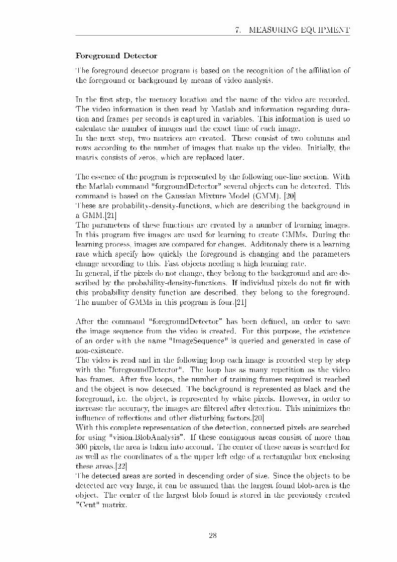
Figure 20: Spring characteristics spring 2, red[19].
After the experiment has been carried out, the weight force of the mass can beplotted against the change in length. This is shown in �gures 19 and 20. Thegradient of the spring characteristic determines the spring sti�ness. This is forspring 1 k1= 35.7 N/m and for spring 2 k2= 28.7 N/m for spring.
26

7. MEASURING EQUIPMENT
7. Measuring Equipment
In this section, the used measuring systems are explained in more detail. Duringthe experiments, the generated waves are recorded as well as the oscillation of thetest objects. Both happend in di�erent ways. While the test objects are detectedby video analysis, the generated waves are detected by capacitive sensors.
Wave Gauges
Three measuring points of the type Wave Sta� XB from Ocean Sensor are usedto collect the wave data.The measuring system is based on the principle of capacity change with changeof water level. For this purpose, the system consists of two separate electrodes.The Te�on insulation of the rod serves as dielectric. While one electrode is inthe water, the second electrode is in the sensor shaft as a shield conductor. If thewater depth changes, the capacity changes linearly. The capacity is recorded asa function of time and can therefore be assigned to a voltage value.
The calibration is carried out by a maximum of 12 measuring points, whichshould be in the range of 20-80% of the expected measuring range of the waterdepth. Each calibration point has a tolerance of 0.05%. During calibration, avoltage value is assigned to each measuring point at a known water depth. Thiscreates a calibration curve that is stored and called up in the system.
Depending on the length of the Shaft, here 0.5 m, water depths that do notexceed this value can be measured.
Measuring Programs
One goal of the experiments is to capture and graphically display the motionbehaviour of the test objects. The position of the object should therefore berecorded over time. In order to realize this technically, the tests were recordedby means of a video camera. These videos can then be analysed using Matlab.For this purpose, two di�erent Matlab programs were implemented.
These two programs use di�erent ways to detect the test objects. The �rst pre-sented program is based on a color detection of the object, the second programon a detection of the movement of the object. However, after the test object hasbeen detected, both programs use the same code.Depending on the enviromental conditions of the recordings, a di�erent programmay be advantageous. If the environmental conditions have many colors, whichare very similar to the test object ist would be di�cult to seperate the test object.On the other hand, if more than the test object is moving in the video, the objectshould be detected by color seperation.
Motion Tracker 2 was used to analyze the data presented here. This has thebackground that the wave movement can be seen in the videos.
27
7. MEASURING EQUIPMENT
Foreground Detector
The foreground detector program is based on the recognition of the a�liation ofthe foreground or background by means of video analysis.
In the �rst step, the memory location and the name of the video are recorded.The video information is then read by Matlab and information regarding dura-tion and frames per seconds is captured in variables. This information is used tocalculate the number of images and the exact time of each image.In the next step, two matrices are created. These consist of two columns androws according to the number of images that make up the video. Initially, thematrix consists of zeros, which are replaced later.
The essence of the program is represented by the following one-line section. Withthe Matlab command "forgroundDetector" several objects can be detected. Thiscommand is based on the Gaussian Mixture Model (GMM). [20]These are probability-density-functions, which are describing the background ina GMM.[21]The parameters of these functions are created by a number of learning images.In this program �ve images are used for learning to create GMMs. During thelearning process, images are compared for changes. Additonaly there is a learningrate which specify how quickly the foreground is changing and the parameterschange according to this. Fast objects needing a high learning rate.In general, if the pixels do not change, they belong to the background and are de-scribed by the probability-density-functions. If individual pixels do not �t withthis probability-density-function are described, they belong to the foreground.The number of GMMs in this program is four.[21]
After the command "foregroundDetector" has been de�ned, an order to savethe image sequence from the video is created. For this purpose, the existenceof an order with the name "ImageSequence" is queried and generated in case ofnon-existence.The video is read and in the following loop each image is recorded step by stepwith the "foregroundDetector". The loop has as many repetition as the videohas frames. After �ve loops, the number of training frames required is reachedand the object is now detected. The background is represented as black and theforeground, i.e. the object, is represented by white pixels. However, in order toincrease the accuracy, the images are �ltered after detection. This minimizes thein�uence of re�ections and other disturbing factors.[20]With this complete representation of the detection, connected pixels are searchedfor using "vision.BlobAnalysis". If these contiguous areas consist of more than300 pixels, the area is taken into account. The center of these areas is searched foras well as the coordinates of a the upper left edge of a rectangular box enclosingthese areas.[22]The detected areas are sorted in descending order of size. Since the objects to bedetected are very large, it can be assumed that the largest found blob-area is theobject. The center of the largest blob found is stored in the previously created"Cent" matrix.
28
7. MEASURING EQUIPMENT
In the next step, a colored box is inserted around the detected object in the origi-nal image. The previously known position of the box from the vision.blobAnalysiscommand is used. The edited image is saved and then used to analyze the po-sition of a chessboard, which is visible in all videos. The chessboard is used tocalibrate the camera position.
Already 35 pictures from di�erent camera positions have been taken with thechessboard in the designated position for the experiments. These images wereanalyzed using the Matlap "CameraCalibrator" app and the results were storedin the CameraParams variable and the properties of the calibration panel. Toperform this analysis, the size of the chess pattern must be known. It analyzes thecamera distortion and camera properties that describe how the camera createsa 2D image from a three dimensional environment. This is important in orderto later deduce the 3D reality from the images and thus to calculate the actualposition of the test objects in the room. This is not represented realistically bychanging the dimension when it is transformed into a photo.[23]After the analysis is completed, 3D world points can be determined from 2D im-ages using the calculated camera parameters. First, the size of the chessboardand the corner points of all �elds in the chessboard are determined with the com-mand "detectCheckerboardPoints". It is important that the chessboard has adi�erent number of rows and columns to be able to assign whether it is a verticalor horizontal movement. In this step the chess board in the image is simultane-ously compared with the chess board from the calibration. It must be the sameor the program will not continue.In the following command 'extrinics' two correction matrices are created. A 3Drotation matrix and a 3D translation vector. The purpose of these matrices is towrite points from the two-dimensional camera coordinate system ("ImagePoints")into the world coordinate system. The detected points of the chessboard in theimage and the world points as well as the lens distortion from the camera param-eters are used for this. These correction matrices are then used to correct thestored coordinates of the objects in the "Cent" matrix and save them in "World-Cent", thus reproducing the realistic object position.[24]
Afterwards the revised images are written back into a video and saved.Finally, the y-cordiants of the blob from the matrix "WorldCent" are written intoa matrix name "position" using matrix calculations together with the time of therespective frames as x values. The reason for this, is that the matrix "WolrdCent"stores the center of the blobs. However, since there is only a vertical movementof the object, i.e. in the y-direction, the x-cordiants should not change and areof no importance. In order to be able to trace the time-dependent vertical move-ment of the object later and to be able to use it in other programs, it is useful tostore both information, time and vertical position, in a matrix. In this arithmeticoperation, the actual position of the coordinate origin in the chessboard, top left,in relation to the bottom of the shaft tank in the variable E can be taken intoaccount, if desired. The coordinate origin is de�ned by the Calibration App anddisplayed to the user during calibration. The unit of the value for E depends onthe unit of the chessboard in the Calibration App.
29

7. MEASURING EQUIPMENT
Finally, the course of the detected object is displayed graphically.
Motion Tracker 2
Due to the de�ned test conditions of the objects close to the water surface andthe di�culties of the Foregound Detector program to detect only the movementof the test object, a second variant was created. This program is also based onthe Matlab program "Motion Tracker", but this time it is the basic principle ofdetection by color seperation. The program "SimpleColorDetectionByHue" inthe appendix is used as a further source.
As already explained in the previous section, this program �rst asks for the loca-tion, name of the video and the video information, as well as the creation of thematrices for position storage and after a negative query, the folder for saving theimages.
The video is then saved in its image sequence. As this image sequence is changedin the further process to a black and white image, in which the chessboard isno longer visible for correction of the camera position, the video is read againand the corresponding image sequence is called up step by step in the followingfor-loop. Here, too, the loop is run through as often as the video has images.
The previously saved images are called up individually as they pass throughthe loop and read in with the "imread" command. At the same time, the com-mand identi�es the color of each pixel and assigns values to each color and savesthem. These are described in the matrix rgbImage. Some images have a colormap (storedColorMap), in which a value for the color is entered for each pixel.Each pixel in the color map is described by a numeric value.In the next step, the size, i.e. row, columns and number of color bands of thepreviously created matrix are recorded. This is used to later recognize the imagetype of the photo, as the type of photo determines the way the values are assignedto describe a color. If one or more values are to be used to draw conclusions aboutthe color, it must be determined which image type and therefore which color cod-ing is concerned, as well as which image class is concerned. Depending on theclass of the image (uint8, uint16, single, or double), the color values are in a rangeof values between 0 and 1 (double and single), 0 and 255 (uint8) and 0 to 65535(uint16).[25]Uint16 has such high quality for images, that it is not used for normal picturesand this program.In general, there are three di�erent types to describe an image by values. Truecolor Image, indexed image and a grayscale image. A true color images dis-cribes each color with three values. These values are descirbing the terms of thecolour amount of red, green, and blue which are repesented. The second type isa grayscale image, here the color is only described by one numerical value, sincethis is su�cient to clearly identify and delimit the color. Therefore, this type hasonly one color band. This knowledge is later used to identify the image type. Inthe third and last type, the indexed image, the color is the only one which is de-scribed by a vector and a color map. Also in this case, the number of color bandsis equal to one. As for the application of the program, the vector representation
30
7. MEASURING EQUIPMENT
is required by three numerical values of the true colour image, the other cases arechecked in the following.[25]
Based on this background, the system �rst checks which image class is involved.If it is an 8 bit image, the value for uint8 is set to 1. The image type is thenchecked for indexed and geayscale. If the number of colour bands is equal to one,it must be one of these two types. If, in addition to this criterium, a color mapexists, it is an indexed image, otherwise it is a greyscale image.If the conditions of a grayscale image are ful�lled, in the next step the descriptivecolor values are converted into the format of a truecolor image with the command"cat". So instead of one value for a color into three descriptive values for a color.This command does nothing else than copy the one descriptive color value foreach pixel, that at the end three descriptive numerical values with the valence ofthe color value in greyscale format exists. These values then describe exactly thesame color in truecolor format.If an indexed image is identi�ed instead of a greyscale image, then this image typeis also converted to truecolor image. This is done with the command "ind2rgb".However, this command only covers the indexed image to a truecolor image withthe image class double or single. Unlike greyscale images, where the values aresimply copied and the image class is not changed, the image class can be changedwhile converting an indexed uint8 image. This is the reason why it was checkedbefore whether it is an 8 bit image. If this criterion is met, all color values aremultiplied by 256 in the next step and thus returned to uint8.
If it can now be assumed that it is a truecolor image or also called rgb image, thenext step is to convert the color values back to HSV format. HSV describes colorsusing three values for hue, saturation and value. HSV is always preferred when acolour description is required. The reason for this is that the HSV model is moresimilar to the human visual perception and therefore easier to de�ne and selectcolour value ranges. Since the user should later be able to adjust these ranges fordi�erent recording conditions, a color description is necessary. The conversion isinitiated by the command "rgb2hsv".[26]In the following three lines of code, the HSV values are written into the corre-sponding matrix (hImage, sImage and vImage) according to hue, saturation andvalue. The user can then specify his own values for these three color characteris-tics. They are describing the colors that the program is looking for and detecting.In the next step, all values in the three matrices, which are in the desired colorvalue range, are transferred to three new matrices (hueMask, saturationMask andvalueMask). If values are not in the value range, they are stored as zeros in thenew matrices.Now the three matrices hueMask, saturationMask and valueMask are combinedagain as colorObjekctMask. If all three HSV properties have a value for one pixel,they describe the color we are looking for. If only one of these three values iszero, the pixel is not included in the detection.
In order to minimize the in�uence of disturbing factors, all pixel areas that ful�llthe color values but do not have more than 100 neighboring such permitted pix-els, they are eliminated in the following two steps. Furthermore, the edges are
31

7. MEASURING EQUIPMENT
smoothed and individual color values for pixels that could belong to the objectare included.
The following steps are the same as in ForegroundDetector and are thereforenot explained here. With the help of the command blobAnalysis the contiguouspixel area is captured by coordinates and provided with a box. Then the areasare sorted by size and the largest detected area is used for further steps. In theoriginal image a box is then inserted around the pixel area and the coordinates ofthe detected area are corrected with the camera parameters. The image sequenceis merged into a video, the time and the y-coordinates are stored in a variableand plotted.
32

8. ERROR ANALYSIS
8. Error Analysis
To determine the analysis accuracy of the object oscillation, the wave conditionswere repeated three times for test object one with spring one and for all submer-gence depth. It is assumed that the object oscillation must be the same due tothe unchanged parameters for the repetitions.Therefore, the oscillation height of the test object Hoz for all three repetitions hasbeen determined.The deviation of the oscillation height of the repetitions is cac-ulated, Eq.(37), by further analysis of the largest and smallest oscillation heightHoz,max and Hoz,min,as well as the avverage heights Hoz,Averrage. This is referredhere as oscillations height deviation Hoz,error.
𝐻𝑜𝑧,𝑒𝑟𝑟𝑜𝑟 =𝐻𝑜𝑧,𝑚𝑎𝑥 −𝐻𝑜𝑧,𝑚𝑖𝑛
𝐻𝑜𝑧,𝐴𝑣𝑒𝑟𝑟𝑎𝑔𝑒
* 100% (37)
As visible in table 7, the error range is very large. On the whole, no correlationsof the error Hoz,error between the individual submergence depths can be observed.About 90% of the oscillation height errors are in the range of 4-20%. However,per submergence depth are about 2-4 values that exceed this range. In very fewcases, the oscillation height error is twice the mean oscillation height.
Due to the large scattering range of the deviations, the empirical standard devi-ations for test object one, spring one, submergence step one are also calculatedusing equation (38). The index n, used there, denotes the wave height H of 1-6from section 4.. The results are shown in Table 4. This means that the averageoscillation heights vary between 0.1 and 6.5 mm.
𝑠 =
√︃∑︀3𝑖=1(𝐻𝑛,𝑜𝑧,𝑖 −𝐻𝑛,𝑜𝑧,𝐴𝑣𝑒𝑟𝑟𝑎𝑔𝑒)2
3(38)
Table 4: Erroranalysis, standart deviation of circular plate with spring one.
Standart deviation of the oscillation height Hoz,sd [mm]„
spring 1, IS = 0.27 m
H [mm]T [s]
0.70 1.00 1.25 1.50 1.75
10 0.648 2.772 1.603 − −20 0.141 1.667 0.869 2.386 2.108
30 0.450 2.536 2.941 2.863 1.597
40 2.176 6.511 1.910 3.285 3.844
50 2.532 6.341 3.581 5.043 5.453
60 1.715 6.533 2.331 0.805 4.705
In general, as the wave height increases, the distances between the repetitions ofthe measured oscillation heights increase, �gure 21, but there is no in�uence ofthe period on this behavior, �gure 22.
33

8. ERROR ANALYSIS
10 20 30 40 50 60
10
15
20
25
30
35
40
45
H_o
z(m
m)
Erroranalysis Oscillation Height Hoz
Circular Plate Spring 1 IS = 0.27m T=0.70s
Run 1Run 2Run 3
Figure 21: Erroranalysis oscillation heights of the di�erent runs as a function ofthe wave height.
0.6 0.8 1 1.2 1.4 1.6 1.810
11
12
13
14
15
16
17
18
H_o
z(m
m)
Erroranalysis Oscillation Height Hoz
Circular Plate Spring 1 IS = 0.27m H=0.02 m
Run 1Run 2Run 3
Figure 22: Erroranalysis oscillation heights of the di�erent runs as a function ofthe wave period.
34
9. RESULTS AND DISCUSSION
9. Results and Discussion
Based on the error analysis, the test data are analysed and interpreted in moredetail. First, the individual test objects are analysed and compared later on. Dueto the transferability to other test environments, values normalized to the waterdepth are also used here.
Analysis Testobject Circular Plate
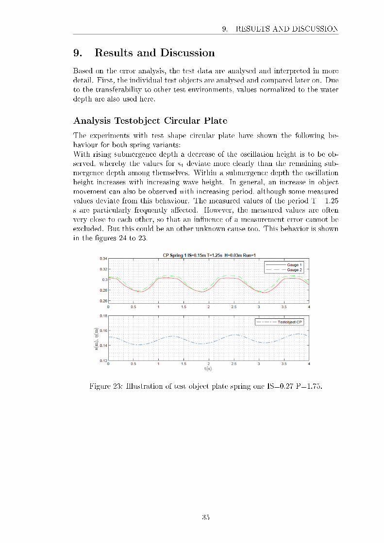
The experiments with test shape circular plate have shown the following be-haviour for both spring variants:With rising submergence depth a decrease of the oscillation height is to be ob-served, whereby the values for s4 deviate more clearly than the remaining sub-mergence depth among themselves. Within a submergence depth the oscillationheight increases with increasing wave height. In general, an increase in objectmovement can also be observed with increasing period, although some measuredvalues deviate from this behaviour. The measured values of the period T= 1.25s are particularly frequently a�ected. However, the measured values are oftenvery close to each other, so that an in�uence of a measurement error cannot beexcluded. But this could be an other unknown cause too. This behavior is shownin the �gures 24 to 23.
Figure 23: Illustration of test object plate spring one IS=0.27 P=1.75.
35
9. RESULTS AND DISCUSSION
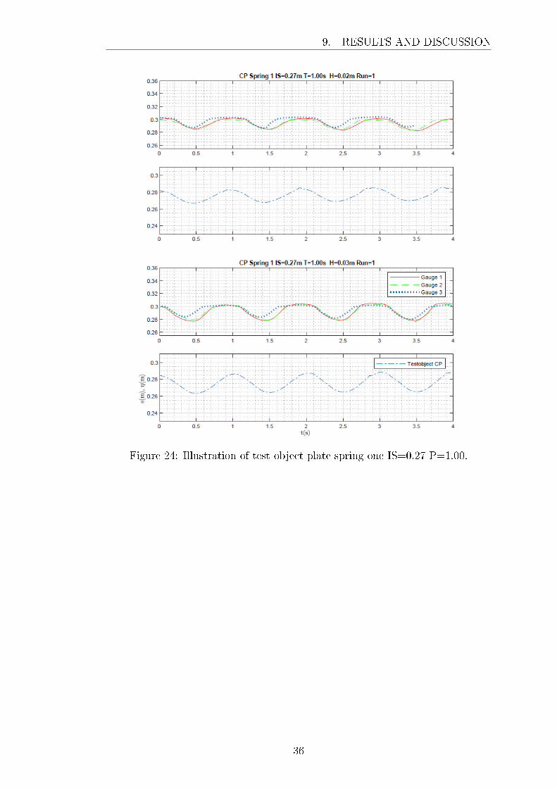
Figure 24: Illustration of test object plate spring one IS=0.27 P=1.00.
36
9. RESULTS AND DISCUSSION
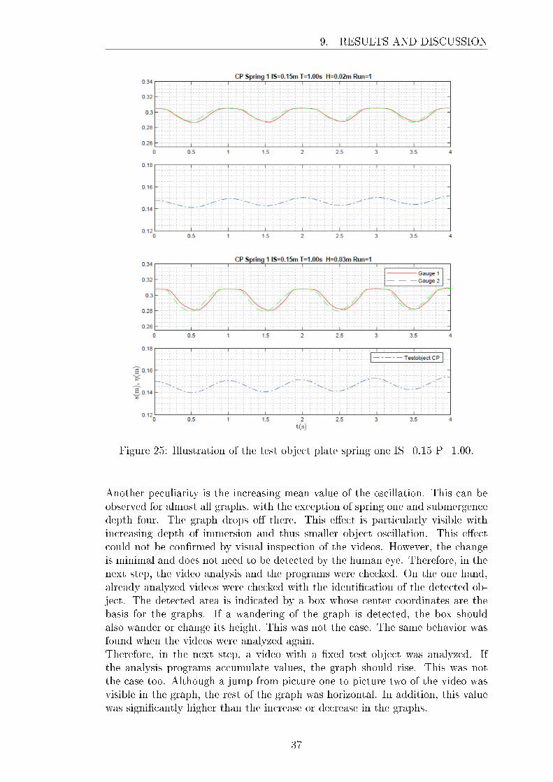
Figure 25: Illustration of the test object plate spring one IS=0.15 P=1.00.
Another peculiarity is the increasing mean value of the oscillation. This can beobserved for almost all graphs, with the exception of spring one and submergencedepth four. The graph drops o� there. This e�ect is particularly visible withincreasing depth of immersion and thus smaller object oscillation. This e�ectcould not be con�rmed by visual inspection of the videos. However, the changeis minimal and does not need to be detected by the human eye. Therefore, in thenext step, the video analysis and the programs were checked. On the one hand,already analyzed videos were checked with the identi�cation of the detected ob-ject. The detected area is indicated by a box whose center coordinates are thebasis for the graphs. If a wandering of the graph is detected, the box shouldalso wander or change its height. This was not the case. The same behavior wasfound when the videos were analyzed again.Therefore, in the next step, a video with a �xed test object was analyzed. Ifthe analysis programs accumulate values, the graph should rise. This was notthe case too. Although a jump from picture one to picture two of the video wasvisible in the graph, the rest of the graph was horizontal. In addition, this valuewas signi�cantly higher than the increase or decrease in the graphs.
37

9. RESULTS AND DISCUSSION
Furthermore, no constant summation within the graphs and among each othercould be determined.
Another point of the oscillation behavior is that the movement behavior of thetest object is gentler than the wave. This means that with a rash of the wave,the object follows this movement in attenuated and smooth.
If one compares the behaviour of the test object with di�erent springs, similaroscillation heights are obtained:
∙ Spring one:
– s1: Hoz/h= 0.015 - 0.15
– s2: Hoz/h= 0.014 - 0.13
– s3: Hoz/h= 0.007 - 0.073
– s4: Hoz/h= 0.004 - 0.042
∙ Spring two:
– s1: Hoz/h= 0.02 - 0.15
– s2: Hoz/h= 0.012 - 0.098
– s3: Hoz/h= 0.006 - 0.077
– s4: Hoz/h= 23*10�-5 - 41*10-4
However, if all value are considerd and not only the minimum and maximum val-ues of the individual submergence depth, the oscillation height, with the strongerspring one, is generally higher than with spring two. You can see this behaviorin comparison to Figure 26. Because the spring constants of both springs areclose to each other and thus the measured values are also close to each other.Deviations of the addressed behaviour could be related to measurement errors.
Another observation is a slight variation of the average value of the object oscilla-tion within a submergence depth by a maximum of 1 cm. This can be attributedto the large water loss of the wave �ume during the experiments.
38

9. RESULTS AND DISCUSSION
Figure 26: Illustration of test object plate spring two.
Table 5: Analysis oszillation Height Object one.
Ratio of wave height to oscillation height, Hoz/h
of the test object 1 spring 1 IS = 0.27 m
H [mm]T [s]
0.70 1.00 1.25 1.50 1.75
10 0.016 0.027 0.015 − −20 0.037 0.049 0.047 0.040 0.057
30 0.060 0.076 0.076 0.084 0.063
40 0.067 0.093 0.100 0.102 0.097
50 0.102 0.118 0.115 0.143 0.111
60 0.109 0.124 0.122 0.143 0.154
Ratio of wave height to oscillation height, Hoz/h
of the test object 1 spring 1 IS = 0.21 m
H [mm]T [s]
0.70 1.00 1.25 1.50 1.75
10 0.014 0.021 0.014 − −20 0.025 0.038 0.038 0.033 0.032
30 0.037 0.055 0.055 0.060 0.056
40 0.049 0.079 0.068 0.072 0.074
50 0.067 0.090 0.075 0.088 0.079
60 0.083 0.111 0.084 0.091 0.130
39

9. RESULTS AND DISCUSSION
Ratio of wave height to oscillation height, Hoz/h
of the test object 1 spring 1 IS = 0.15 m
H [mm]T [s]
0.70 1.00 1.25 1.50 1.75
10 0.007 0.013 0.010 − −20 0.012 0.022 0.024 0.021 0.019
30 0.019 0.035 0.033 0.041 0.037
40 0.029 0.045 0.042 0.057 0.048
50 0.039 0.055 0.049 0.059 0.068
60 0.040 0.064 0.058 0.064 0.073
Ratio of wave height to oscillation height, Hoz/h
of the test object 1 spring 1 IS = 0.09 m
H [mm]T [s]
0.70 1.00 1.25 1.50 1.75
10 0.004 0.007 0.007 − −20 0.008 0.016 0.017 0.017 0.020
30 0.010 0.021 0.021 0.028 0.020
40 0.014 0.026 0.026 0.035 0.031
50 0.019 0.033 0.037 0.042 0.037
60 0.023 0.039 0.038 0.042 0.041
Ratio of wave height to oscillation height, Hoz/h
of the test object 1 spring 2 IS = 0.27 m
H [mm]T [s]
0.70 1.00 1.25 1.50 1.75
10 0.020 0.029 0.018 − −20 0.034 0.047 0.047 0.044 0.046
30 0.059 0.067 0.068 0.088 0.073
40 0.082 0.088 0.090 0.107 0.091
50 0.081 0.103 0.112 0.125 0.124
60 0.103 0.123 0.127 0.153 0.122
40
9. RESULTS AND DISCUSSION
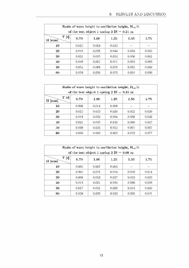
Ratio of wave height to oscillation height, Hoz/h
of the test object 1 spring 2 IS = 0.21 m
H [mm]T [s]
0.70 1.00 1.25 1.50 1.75
10 0.012 0.019 0.013 − −20 0.018 0.035 0.044 0.034 0.035
30 0.031 0.055 0.054 0.056 0.061
40 0.049 0.067 0.071 0.092 0.069
50 0.054 0.086 0.070 0.091 0.086
60 0.070 0.098 0.079 0.094 0.090
Ratio of wave height to oscillation height, Hoz/h
of the test object 1 spring 2 IS = 0.15 m
H [mm]T [s]
0.70 1.00 1.25 1.50 1.75
10 0.006 0.014 0.006 − −20 0.012 0.023 0.026 0.021 0.029
30 0.019 0.034 0.034 0.036 0.042
40 0.025 0.045 0.046 0.060 0.057
50 0.030 0.055 0.055 0.061 0.067
60 0.036 0.069 0.063 0.072 0.077
Ratio of wave height to oscillation height, Hoz/h
of the test object 1 spring 2 IS = 0.09 m
H [mm]T [s]
0.70 1.00 1.25 1.50 1.75
10 0.002 0.007 0.004 − −20 0.005 0.015 0.014 0.016 0.014
30 0.009 0.019 0.017 0.023 0.023
40 0.013 0.027 0.024 0.030 0.028
50 0.017 0.031 0.029 0.034 0.035
60 0.020 0.038 0.033 0.038 0.041
41

9. RESULTS AND DISCUSSION
Analysis Testobject Cone
Unlike test object one, test object two was only tested with spring two and waveheight H6. Here, too, a decline in the association of objects can be observed withincreasing submergence depth. How the oscillation behavior of a continuouslysubmerged test object behaves with increasing submergence depth must be in-vestigated by further tests.
An increase in oscillazion with the period can only be observed for s0, how-ever, when viewing the videos a stuttering oscillation can be observed, which isobviously caused by friction of the tilting bearing. Due to the limitted test of theobject, these tests could not be repeated. It is to be assumed that these are alsothe cause for the strongly falling oscillation heights and thus the statement of thedecreasing oscillation should be checked again. Based on primary observations ofthe behaviour of the test object, increasing oscillation heights are also expectedfor rising wave heights.
Figure 27: Illustration of the test object cone spring two.
During the experiments, weight was increased by water adsorption. The weightincrease in the timeframe of the periods P1 to P5 from s0 was 24 g. And in thesame period from s1 34 g.
∙ Spring two:
– s0: Hoz/h= 0.016 - 0.059
– s1: Hoz/h= 0.006 - 0.067
Table 6: Analysis oszillation Height Object two.
Ratio of wave height to oscillation height, Hoz/h
of the test object 2 spring 2 IS = 0.30 m
H [mm]P [s]
0.70 1.00 1.25 1.50 1.75
60 .016 .057 .059 .055 .041
42
9. RESULTS AND DISCUSSION
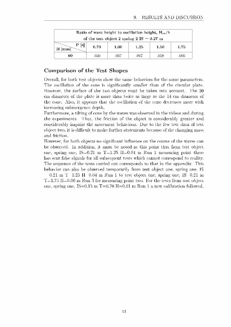
Ratio of wave height to oscillation height, Hoz/h
of the test object 2 spring 2 IS = 0.27 m
H [mm]P [s]
0.70 1.00 1.25 1.50 1.75
60 .030 .067 .067 .018 .006
Comparison of the Test Shapes
Overall, for both test objects show the same behaviors for the same parameters.The oscillation of the cone is signi�cantly smaller than of the circular plate.However, the surface of the two objects must be taken into account. The 30cm diameter of the plate is more than twice as large as the 14 cm diameter ofthe cone. Also, it appears that the oscillation of the cone decreases more withincreasing submergence depth.Furthermore, a tilting of cone by the waves was observed in the videos and duringthe experiments. Thus, the friction of the object is considerably greater andconsiderably impairs the movement behaviour. Due to the few test data of testobject two, it is di�cult to make further statements because of the changing massand friction.However, for both objects no signi�cant in�uence on the course of the waves canbe observed. In addition, it must be noted at this point that from test objectone, spring one, IS=0.21 m T=1.25 H=0.04 m Run 1 measuring point threehas sent false signals for all subsequent tests which cannot correspond to reality.The sequence of the tests carried out corresponds to that in the appendix. Thisbehavior can also be observed temporarily from test object one, spring one, IS= 0.21 m T=1.25 H=0.04 m Run 1 to test object one, spring one, IS=0.21 mT=1.75 H=0.06 m Run 3 for measuring point two. For the tests from test objectone, spring one, IS=0.15 m T=0.70 H=0.01 m Run 1 a new calibration followed.
43

10. CONCLUSION
10. Conclusion
Due to the increasing energy consumption, the decreasing fossil fuel resources andclimate change, renewable energies are becoming increasingly important. Waveenergy in particular represents one of the largest and at the same time mostunutilized resource and therefore o�ers a lot of potential. Many projects to gen-erate wave energy are still in the R&𝐷-stage. This thesis is intended to make acontribution to this.
The aim of this bachelor thesis was to determine the oscillation behavior of variousforms of submerged primer movers, which are used as a component in heavingWEC. This was done experimentally in a wave �ume and under the in�uenceof shallow water and various submergence depth, wave period, wave height andspring sti�ness. Test environment was a piston-wave-maker. The test setup wasdesigned in such a way that the objects were mounted on a shaft with a lin-ear bearing and a spring. This shaft was �xed in vertical position in the wave�ume. Two measuring points for measuring the waves were located upwave andone downwave. Two test objects were used. A circular 3 mm thick plate and acone. The shape of the cone is based on scienti�c research on asymmetric, heav-ing devices on the water surface.
Wireless capacitive measuring systems were used as measuring instruments todetermine the water depth as a function of time. Thus, the wave movementscan be captured. The motion detection of the test objects was based on videorecordings which were analyzed by means of two programs. These programs usethe Matlab interface and are based on color seperation and recognition of thebackground by mathematical Gaussian Mixture Models. Mainly the software,which is based on color seperation was used.
The error range determined during the analysis of the experiments is very large.About 90% of the test values show an error of 4 - 20%. Related to the test, thisis a variation of the object oscillation of 0.1 - 6.5 mm with wave height of 1 to6 cm. The deviations increase with increasing wave height as well as to a largeextent with increasing wave period.
The following behavioural statements and correlations can be made for the testobjects themselves:Both, for the circular plate and for the cone, the object oscialltion increaseswith increasing wave height and, for the most parts, with increasing wave period.Whereas with increasing submergence depth the object oscillation decreases. Fur-thermore, the oscillation seems to be larger with greater spring sti�ness. Theoscillation of the test objects does not seem to have any signi�cant in�uence onthe progression of the waves.In addition, it can be observed that the oscillation of the circular plate is greaterfor the same test parameters than the oscialltion of the cone. However, the coneis signi�cantly smaller in relation to the relevant surfaces for the forces than theplate.
44

10. CONCLUSION
It is recommended to carry out further tests with the test object cone in or-der to have more comparable data with the plate. In relation to the cone, thebasic behavior should also be observed with a larger dimensioning and a largerdi�erence between the upper and the bottom diameter.
45

REFERENCES
References
[1] MathWorks. Detecting cars using gaussian mixture mod-els. https://de.mathworks.com/help/vision/examples/
detecting-cars-using-gaussian-mixture-models.html, 2018.[acess:27.06.2018].
[2] Dr. Masoud Hayatdavoodi. Motion tracker. Unpublished, March 2018. Mat-lab Program.
[3] MathWorks. Simple color detection by hue. https://de.mathworks.com/
matlabcentral/fileexchange/28512-simplecolordetectionbyhue?
focused=5807952&tab=function, 2018. [acess:02.07.2018].
[4] WON Linear Motion System. Linear Ball Bushing. WON Linear Motion Sys-tem, http://www.lunabearings.com/new/Linear_Ball_Bushing.pdf edi-tion. [Online; accessed 09-June-2018].
[5] Klaus Gebhardt. Das umweltlexikon�erneuerbare energien.https://www.umweltdatenbank.de/cms/lexikon/31-lexikon-e/
1690-erneuerbare-energie.html, 2018. [Online; accessed 06-August-2018].
[6] H.C.Soerensen Erik Friis-Madsen and S. Parmeggiani. Wave dragon. Pre-sentation, 2012.
[7] Cibran Camba Rey Augusto Barata da Rocha, John Dalen Marc Le Boul-luec (Chair), Finn Gunnar Nielsen Henry Je�rey, Nathalie Rousseau Geof-frey O'Sullivan, Eoin Sweeney, and Judith Wolf . Marine renewable energyresearch challenges and opportunities for a new energy era in europe. printed,online, October 2010.
[8] Gail Tverberg. The energy collective. http://
www.theenergycollective.com/gail-tverberg/2396261/
2017-the-year-when-the-world-economy-starts-coming-apart, 2018.[Online; accessed 28-May-2018].
[9] Robin Pelc and Rod M. Fujita. Renewable energy from the ocean. Marine
Policy, 26(6):471�479, November 2002.
[10] Alain Clément, Pat McCullen, Antonio Falcao, Antonio Fiorentino,Fred Gardner, Karin Hammarlund, Georgios Lemonis, Tony Lewis, KimNielsen, Simona Petroncini, M.-Teresa Pontes, Phillippe Schild, Bengt-OlovSjöström, Hans Christian Sørensen, and Tom Thorpe. Wave energy in eu-rope: Current status and perspectives. 6:405�431, 10 2002.
[11] Frank Neumann (IMIEU) Ruud Kempener (IRENA). Wave energy tech-nology brief. Printed, IRENA Innovation and Technology Centre Robert-Schuman-Platz 3 53175 Bonn Germany, June 2014.
[12] Simona Negro, Floortje Alkemade, and Marko Hekkert. Renewabale andsustainable energy reviews. Elsevier, 16, January 2012.
46

REFERENCES
[13] Shuijin Li. Structual analysis of a wave energy device. Master's thesis,University of Dundee, School of Science and Engineering, March 2017.
[14] Malin Goteman Liguo Wang, Jens Engstrom and Jan Isberg. Constrainedoptimal control of a point absorber wave energy converter with linear gen-erator. JOURNAL OF RENEWABLE AND SUSTAINABLE ENERGY,Volume 7, 2015.
[15] Prof. S. A. Sannasiraj. Module ii laboratory wave generation.
[16] Turgut Sarpkaya and Michael Isaacson. Mechanics of wave forces on offshore
structures. Van Nostrand Reinhold Co New York, 1981.
[17] Farshad Madhi, M.E. Sinclair, and Ronald Yeung. The �berkeley wedge�:an asymmetrical energy-capturing �oating breakwater of high performance.9:5�16, 01 2014.
[18] M. Hayatdavoodi, K. Treichel, and R. C. Ertekin. Parametric study of non-lineae wave loads on submerged decks in shallow water. Preprint submit-ted, manuscript obtained through personal communication with Dr. Hayat-davoodi., 2018.
[19] Xiachen Zhang. Laboratory test of a submerged wave energy device. Master'sthesis, School of science and engineering, August 2018.
[20] MathWorks. Foreground detection using gaussian mixture models - mat-lab - mathworks deutschland. https://de.mathworks.com/help/vision/
ref/vision.foregrounddetector-system-object.html, 2018. [Online;accessed 09-June-2018].
[21] Yannick Benezeth, Pierre-Marc Jodoin, Bruno Emile, Hélène Laurent, andChristophe Rosenberger. Comparative study of background subtraction al-gorithms. Journal of Electronic Imaging, 2010.
[22] MathWorks. vision.blobanalysis system object- properties of connectedregions - matlab - mathworks deutschland. https://de.mathworks.com/
help/vision/ref/vision.blobanalysis-system-object.html, 2018.[Online; accessed 01-July-2018].
[23] MathWorks. Single camera calibrator app - matlab & simulink -mathworks deutschland. https://de.mathworks.com/help/vision/ug/
single-camera-calibrator-app.html, 2018. [Online; accessed 01-June-2018].
[24] MathWorks. Determine world coordinates of image points - matlabpointstoworld - mathworks deutschland. https://de.mathworks.com/
help/vision/ref/cameraparameters.pointstoworld.html, 2018. [On-line; accessed 01-June-2018].
[25] MathWorks. Image types - matlab & simulink - mathworksdeutschland. https://de.mathworks.com/help/vision/ref/vision.
blobanalysis-system-object.html, 2018. [Online; accessed 01-July-2018].
47

REFERENCES
[26] MathWorks. Convert rgb colors to hsv - matlab rgb2hsv - mathworksdeutschland. https://de.mathworks.com/help/matlab/ref/rgb2hsv.
html, 2018. [Online; accessed 11-June-2018].
48

Appendix
List of Appendix
A. Messuring Program Foreground Detector . . . . . . . . . . . . . . . . . . . . . . . . . . . 50
B. Messuring Program Motion Track 2 . . . . . . . . . . . . . . . . . . . . . . . . . . . . . . . . 54
C. Submittal Messuring Program Motion Tracker . . . . . . . . . . . . . . . . . . . . . 60
D. Basic Load Ratings Linear Bearings . . . . . . . . . . . . . . . . . . . . . . . . . . . . . . . . 63
E. Example Excerpt of Plots Erroranalysis oscillation Height . . . . . . . . . . 64
F. Plots Oscillation Height Testobject Circular Plate . . . . . . . . . . . . . . . . . . 67
G. Plots Oscillation Height Testobject Cone . . . . . . . . . . . . . . . . . . . . . . . . . . . 147
49

%%
%% INTRODUCTION
% This program was written to detect the movements of objects by means of a
% video recording and thus to determine the exact position. The course of
% movement is detected, the object is highlighted and the position data is
% saved and output as a diagram.
%
% This program is partly based on a program called "motiontracker" by
% Dr. Masoud Hayatdavoodi from the University of Dundee and a program
% example by Matlab
% (https://www.mathworks.com/help/vision/examples/detecting-cars-using-
gaussian-mixture-models.html)[acess:27.06.2018].
%
% Author: Linda Eckel (Universitaet der Bundeswehr Muenchen)
% 01/06/2018
%%
%%---------------------------Input-----------------------------------------%
% Change the following directory to where your video files are.
cd('C:\');
videoName = 'MVI.mov'; % Name of the movie file.
cameraParameters = 'cameraParams.mat' % Name of file with the cameraparameters from the
Camera Calibration App.
%%
%%---------------------------Variable---------------------------------------%
% Reading and loading cameraparameters
exist cameraParams % Check existence in workspace
if ans~=1 % If non-existence, load parameters.
load 'cameraParams.mat'
A. Messuring Program Foreground Detector
Figure 28: Messuring Program Foreground Detector[1],[2].
50

end
motionVideo = VideoReader(videoName);
h = waitbar(0,'Please wait');
fps = motionVideo.FrameRate; %Reading frames per seconds
T = motionVideo.Duration; %Reading period
numFrames = round(fps*T); %Calculate numbers of frames in video
time = 0:1/fps:T-(1/fps); %Calculate time of video
% Counting variables
ii = 1;
jj = 1;
k = 1;
% Checkboard position
e=220;% 220mm from lowest point of chessboard (origin of the
% coordinatesystem of the plot) to the bottom of the wavemaker.
% Use mm if you are using mm for the chessboard size in camera calibrator too.
%%
%%----------------------------Matrix-----------------------------------------%
cent = zeros(numFrames,2);
worldCent = zeros(numFrames,2);
%%
%%--------------------------Start--Programm----------------------------------%
foregroundDetector = vision.ForegroundDetector('NumGaussians', 4, ...
'MinimumBackgroundRatio', 0.09, 'NumTrainingFrames', 5, 'LearningRate', 0.0001 );
% Proof existing file to safe images in it. If non-existence, create file.
exist Image_Sequence
if ans~=7
51

mkdir Image_Sequence % Creates folder for the extracted frames
end
videoReader = vision.VideoFileReader(videoName);
for jj = 1:numFrames;
waitbar(jj/numFrames,h,'Waiting for Detecting Foreground');
% Detect foreground: Moving object will be in white pixels, background
% in black
frame = step(videoReader); %Read the next video frame
foreground = step(foregroundDetector, frame);%Detect foreground
% Filtered detected foreground for better quality
se = strel('square', 3);
filteredForeground = imopen(foreground, se);
% Find areas of white pixels which are bigger then 300 pixels
blobAnalysis = vision.BlobAnalysis('AreaOutputPort', true,...
'CentroidOutputPort', true,...
'BoundingBoxOutputPort', true,...
'MinimumBlobArea', 300, 'ExcludeBorderBlobs', false);
[areas, centroids , boxes] = step(blobAnalysis, foreground);
% Sort areas with white pixels in descending rder
[~, idx] = sort(areas, 'Descend');
% Get the two largest areas.
if numel(boxes) > 0
boxes = double(boxes(idx(1), :));
cent(jj,:) = double(centroids(idx(1),:));
end
52

% Insert box in coloured Frames
imDetectedObj = insertObjectAnnotation(frame, 'rectangle', ...
boxes, 'Object');
% Save Frames with Boxes
filename=strcat('frame',num2str(jj),'.jpg');
folder = 'Image_Sequence';
fullname = fullfile(folder,filename);
imwrite(imDetectedObj,fullname);
% Detect the checkerboard.
[imagePoints, boardSize] = detectCheckerboardPoints(frame);
% Compute rotation and translation of the camera.
[R, t] = extrinsics(imagePoints, cameraParams.WorldPoints, cameraParams);
% Get the world coordinates of the corners
worldCent(jj,:) = pointsToWorld(cameraParams, R, t, cent(jj,:));
jj = jj+1;
end
%%
% Write the processed frames back to a video file
imageNames = dir(fullfile('Image_Sequence','*.jpg'));
imageNames = {imageNames.name}';
outputVideo = VideoWriter(fullfile('motiontrack66.avi'));
outputVideo.FrameRate = motionVideo.FrameRate;
open(outputVideo)
for ii = 1:length(imageNames)
img = imread(fullfile('Image_Sequence',imageNames{ii}));
writeVideo(outputVideo,img)
waitbar(ii/numFrames,h,'Reconstructing video');
53

%% %% INTRODUCTION % This program was written to detect the movements of objects by means of a % video recording and thus to determine the exact position. The course of % movement is detected, the object is highlighted and the position data is % saved and output as a diagram. % % The program is partly based on a program called "motiontracker" by % Dr. Masoud Hayatdavoodi from the University of Dundee and a program % example by called "SimpleColorDetectionByHue" % (https://uk.mathworks.com/matlabcentral/fileexchange/28512- % simplecolordetectionbyhue--?focused=5807952&tab=function)[acess: 02.07.2018]. % % Author: Linda Eckel (Universitaet der Bundeswehr Muenchen) % 01/06/2018 %% %%---------------------------Input-----------------------------------------% % Change the following directory to where your video files are. cd('E:\MATLAB-Programme\NeuesProgramm'); % Location of the video fileand the camera parameters videoName = '1_1_070_6_1.mov'; % Name of the movie file. %--------------------------------------------------------------------------% %% %%---------------------------Variable--------------------------------------% % Reading and loading cameraparameters exist cameraParams %Check existence in workspace if ans~=1 %If non-existence, load parameters. load ('cameraParams.mat') end % load(cameraParameters) motionVideo = VideoReader(videoName); h = waitbar(0,'Please wait'); fps = motionVideo.FrameRate; % Reading frames per seconds T = motionVideo.Duration; % Reading period numFrames = round(fps*T); % Calculate numbers of frames in video time = 0:1/fps:T-(1/fps); % Calculate time of video % Counting variables ii = 1; jj = 1; kk = 1; % Checkboard position e=220;% 220mm from origin of the origin of the coordinatesystem % (upper left site) to the bottom of the wavemaker. Use mm if you are using % mm for the chessboard size in camera calibrator too. %%
B. Messuring Program Motion Track 2
Figure 29: Messuring Program Motion Track 2[3],[2].
54

%%----------------------------Matrix-----------------------------------------% cent = zeros(numFrames,2); worldCent = zeros(numFrames,2); %% %%--------------------------Start--Programm----------------------------------% %Proof existing file to safe images in it. If non-existence, create file. exist Image_Sequence if ans~=7 mkdir Image_Sequence %Creates folder for the extracted frames end % Cut video into picture squence and save them. while kk<=numFrames waitbar(kk/numFrames,h,'Extracting frames from video'); img = readFrame(motionVideo); filename = [sprintf('%03d',kk) '.jpg']; % Filname (001, 002, ...) folder = 'Image_Sequence'; % Storage location fullname = fullfile(folder,filename); imwrite(img,fullname) % Write out to a JPEG file with filname in folder kk = kk+1; end % Read video again.Reads the video again, because the generated images of % the folder "Image_Sequence" are changed to black and white images when the % object is detected. Only the object which is detected is displayed as % white pixels. For better visual inspection of which object has been % identified, the yellow box, that marks the found object, is inserted into % original images. videoReader = vision.VideoFileReader(videoName); % Detecing Object for jj = 1:numFrames; waitbar(jj/numFrames,h,'Detecting and Tracking Movement of Object'); filename = [sprintf('%03d',jj) '.jpg']; folder = 'Image_Sequence' fullname = fullfile(folder,filename); % Identifies the color of each pixel and assigns values to each colour. % These arrays are describing. Some pictures have a colour chart where is % inetered in each pixel one value for the colour. Thus, every pixel in % the colour map has a numerical value that describes it. %%%%%%%%%%%%%%%%%%%%%%%%%%%%%%%%%%%%%%%%%%%%%%%%%%%%%%%%%%%%%%%%%%%%%%%%%%%%%%%%%%%%%%%%%%%%%%%%%%%%%%%%%%%%%%%%%%%%%%%%%%%%%%%% % This section is subject to the following copyright laws: %Copyright (c) 2015, Image Analyst %Copyright (c) 2018, Image Analyst %All rights reserved.
55

%Redistribution and use in source and binary forms, with or without %modification, are permitted provided that the following conditions are met: %* Redistributions of source code must retain the above copyright notice, this % list of conditions and the following disclaimer. %* Redistributions in binary form must reproduce the above copyright notice, % this list of conditions and the following disclaimer in the documentation % and/or other materials provided with the distribution %THIS SOFTWARE IS PROVIDED BY THE COPYRIGHT HOLDERS AND CONTRIBUTORS "AS IS" %AND ANY EXPRESS OR IMPLIED WARRANTIES, INCLUDING, BUT NOT LIMITED TO, THE %IMPLIED WARRANTIES OF MERCHANTABILITY AND FITNESS FOR A PARTICULAR PURPOSE ARE %DISCLAIMED. IN NO EVENT SHALL THE COPYRIGHT OWNER OR CONTRIBUTORS BE LIABLE %FOR ANY DIRECT, INDIRECT, INCIDENTAL, SPECIAL, EXEMPLARY, OR CONSEQUENTIAL %DAMAGES (INCLUDING, BUT NOT LIMITED TO, PROCUREMENT OF SUBSTITUTE GOODS OR %SERVICES; LOSS OF USE, DATA, OR PROFITS; OR BUSINESS INTERRUPTION) HOWEVER %CAUSED AND ON ANY THEORY OF LIABILITY, WHETHER IN CONTRACT, STRICT LIABILITY, %OR TORT (INCLUDING NEGLIGENCE OR OTHERWISE) ARISING IN ANY WAY OUT OF THE USE %OF THIS SOFTWARE, EVEN IF ADVISED OF THE POSSIBILITY OF SUCH DAMAGE. [rgbImage, storedColorMap] = imread(fullname); [rows, columns, numberOfColorBands] = size(rgbImage); % The image can be of class uint8, uint16, single, or double. % If it's monochrome (indexed), convert it to color. % Check to see if it's an 8-bit image needed later for scaling. if strcmpi(class(rgbImage), 'uint8') % Flag for 256 gray levels. eightBit = true; else eightBit = false; end % There are three image Types. True color Image, indexed image and a % grayscale image. A true color images discribes each color with three % values. These values are descirbing the terms of the colour amount of % red, green, and blue which are repesented. Depending on the class of the % array (uint8, uint16, single, or double), the values are in a range of % values between 0 and 1 (double and single), 0 and 255 (uint8) and 0 to % 65535 (uint16). Uint16 has such high quality, that it will not use for % normal pictures and this program. The second type is a grayscale image, % here the color is only described by a numerical value, since this is % sufficient to clearly identify and delimit the color. In the third and % last type, the indexed image, the color is the only one described by a % vector and a color map. As for the application of the program the vector % representation is required by three numerical values of the true colour
56

% image, the other cases are checked. % Check if it is a grayscale image. If this is the case, the color has only % one value, this value is sufficient to describe the color. However, since % three values are required everywhere, the missing two numerical values are % added by using the first value. This discribes the same color. if numberOfColorBands == 1 if isempty(storedColorMap) % Just a simple gray level image, not indexed with a stored color map. % Create a 3D true color image where we copy the monochrome image into all 3 (R, G, & B) color planes. rgbImage = cat(3, rgbImage, rgbImage, rgbImage); else % It's an indexed image because the color map is not empty. rgbImage = ind2rgb(rgbImage, storedColorMap); % ind2rgb() will convert it to double and normalize it to the range 0-1. % Convert back to uint8 in the range 0-255, if needed. if eightBit rgbImage = uint8(255 * rgbImage); end end end % Convert RGB image to HSV. HSV describes the properties hue, % saturation and value using three values.It the color description of % importance, HSV model is preferred to RGB model. The reason for this % is that the HSV model is more similar to the human visual perception % and therefore easier to define and select colour value ranges. hsvImage = rgb2hsv(rgbImage); % Extract out the H, S, and V images individually hImage = hsvImage(:,:,1); sImage = hsvImage(:,:,2); vImage = hsvImage(:,:,3); % Assign the low and high thresholds for each color band. % Take a guess at the values that might work for the image. hueThresholdLow = 0.09; hueThresholdHigh = 0.18; saturationThresholdLow = 0; saturationThresholdHigh = 0.7; valueThresholdLow = 0.3; valueThresholdHigh = 1.0; % Now apply each color band's particular thresholds to the color band hueMask = (hImage >= hueThresholdLow) & (hImage <= hueThresholdHigh); saturationMask = (sImage >= saturationThresholdLow) & (sImage <= saturationThresholdHigh); valueMask = (vImage >= valueThresholdLow) & (vImage <= valueThresholdHigh); % Combine the masks to find where all 3 are "true."
57

coloredObjectsMask = uint8(hueMask & saturationMask & valueMask); % Tell user that we're going to filter out small objects. smallestAcceptableArea = 100; % Get rid of small objects. coloredObjectsMask = uint8(bwareaopen(coloredObjectsMask, smallestAcceptableArea)); % Smooth the border using a morphological closing operation, imclose(). structuringElement = strel('disk', 4); coloredObjectsMask = imclose(coloredObjectsMask, structuringElement); % Fill in any holes in the regions. coloredObjectsMask = imfill(logical(coloredObjectsMask), 'holes'); %The section of the copyrights above end here. %%%%%%%%%%%%%%%%%%%%%%%%%%%%%%%%%%%%%%%%%%%%%%%%%%%%%%%%%%%%%%%%%%%%%%%%%%%%%%%%%%%%%%%%%%%%%%%%%%%%%%%%%%%% % Findig connecting components which have more than 300 pixels. blobAnalysis = vision.BlobAnalysis('AreaOutputPort', true,... 'CentroidOutputPort', true,... 'BoundingBoxOutputPort', true,... 'MinimumBlobArea',300, 'ExcludeBorderBlobs', false); [areas, centroids , boxes] = step(blobAnalysis, coloredObjectsMask); % Sort connected components in descending order by area [~, idx] = sort(areas, 'Descend'); % Get the two largest components. if numel(boxes) > 0 boxes = double(boxes(idx(1), :)); cent(jj,:) = double(centroids(idx(1),:)); end % Use original images which has not been changed by color recognition. frame = step(videoReader); % Insert box to show detected area. imDetectedObj = insertObjectAnnotation(frame, 'rectangle', ... boxes, 'Object'); % Save original image with tagged object filename2 = [sprintf('%03d',jj) '.jpg']; folder = 'Image_Sequence'; fullname2 = fullfile(folder,filename2); imwrite(imDetectedObj,fullname2); % Detect the checkerboard. [imagePoints, boardSize] = detectCheckerboardPoints(frame);
58

% Compute rotation and translation of the camera. [R, t] = extrinsics(imagePoints, cameraParams.WorldPoints, cameraParams); % Get the world coordinates of the corners worldCent(jj,:) = pointsToWorld(cameraParams, R, t, cent(jj,:)); jj = jj+1; end % Write the processed frames back to a video file imageNames = dir(fullfile('Image_Sequence','*.jpg')); imageNames = {imageNames.name}'; outputVideo = VideoWriter(fullfile('Motiontrack.avi')); outputVideo.FrameRate = motionVideo.FrameRate; open(outputVideo) for ii = 1:length(imageNames) img = imread(fullfile('Image_Sequence',imageNames{ii})); writeVideo(outputVideo,img) waitbar(ii/numFrames,h,'Reconstructing video'); end close(outputVideo) motiontrack = VideoReader(fullfile('Motiontrack.avi')); ii = 1; while hasFrame(motiontrack) mov(ii) = im2frame(readFrame(motiontrack)); ii = ii+1; waitbar(ii/numFrames,h,'Creating new video'); end %% %Creating matrix only with time and y-values in consideration of the %position of the chessboard. worldCent=worldCent*(-1); a=ones(numFrames,1); b=[0 e]; c=a*b; d=worldCent+c; e=[0 0; 0 1]; x=d*e; position=transpose(time)+x; % Matrix with time and position %% %Save matrix with time and position of the object %inform about saving file message = sprintf('Save Object Position?\nContinue?'); reply = questdlg(message, 'Continue', 'OK', 'Cancel', 'OK'); if strcmpi(reply, 'Cancel') % User said cancel, so exit. else [file, path] = uiputfile('test.xls','Speichern');
59

%% CODE INTRODUCTION
% This script tracks the motion of the oscillating plate in the videofile
% supplied in the current directory. The motion is stored in the
% worldCent variable.
% Read and write video frames as JPEGS in the Image_Sequence folder
% THIS VERSION IS PROVIDED BY DR. HAYATDAVOODI
% 30/03/2018
%% ---------------------------input-----------------------------------------%
% Change the following directory to where your files are.
cd('C:\Users\l.eckel1\Documents\Bundeswehr\Uni\Bachelorarbeit\MATLAB-
Programme\MATLAB_ForegroundDetector');
waitbar(jj/numFrames,h,'Tracking the motion');
fullname = fullfile('Image_Sequence',filename);
imwrite(imDetectedObj,fullname);
videoName = 'combine.MOV'; % Name of the movie file.
%-------------------------------------------------------------------------%
clc
motionVideo = VideoReader(videoName);
ii = 1;
jj = 1;
h = waitbar(0,'Please wait');
fps = motionVideo.FrameRate;
T = motionVideo.Duration;
numFrames = round(fps*T);
time = 0:1/fps:T-(1/fps);
kk=1;
C. Submittal Messuring Program Motion Tracker
Figure 30: Submittal Messuring Program Motion Tracker[2].
60

while kk<=numFrames
img = readFrame(motionVideo);
filename = [sprintf('%03d',kk) '.jpg'];
folder = 'Image_Sequence';
fullname = fullfile(folder,filename);
imwrite(img,fullname) % Write out to a JPEG file (img1.jpg, img2.jpg, etc.)
kk = kk+1;
waitbar(kk/numFrames,h,'Extracting frames from video');
end
cent = zeros(numFrames,2);
worldCent = zeros(numFrames,2);
while jj <= numFrames
% Undistort current frame
filename = [sprintf('%03d',jj) '.jpg'];
imOrig = imread(fullfile('Image_Sequence',filename));
%[im, newOrigin] = undistortImage(imOrig, cameraParams, 'Outputview', ...
'full');
% Segment out foreground based on color space
imHSV = rgb2hsv(imOrig);
saturation = imHSV(:,:,2);
g = graythresh(saturation);
imObj = (saturation > g);
% Find connected components.
61

blobAnalysis = vision.BlobAnalysis('AreaOutputPort', true,...
'CentroidOutputPort', true,...
'BoundingBoxOutputPort', true,...
'MinimumBlobArea', 300, 'ExcludeBorderBlobs', false);
[areas, centroids , boxes] = step(blobAnalysis, imObj);
% Sort connected components in descending order by area
[~, idx] = sort(areas, 'Descend');
% Get the two largest components.
if numel(boxes) > 0
boxes = double(boxes(idx(1), :));
cent(jj,:) = double(centroids(idx(1),:));
end
imDetectedObj = insertObjectAnnotation(im, 'rectangle', ...
boxes, 'Object');
waitbar(jj/numFrames,h,'Tracking the motion');
fullname = fullfile('Image_Sequence',filename);
imwrite(imDetectedObj,fullname)
% Convert image space to real world Euclidean space
% Detect the checkerboard.
[imagePoints, boardSize] = detectCheckerboardPoints(im);
% Compute rotation and translation of the camera.
[R, t] = extrinsics(imagePoints, cameraParams.WorldPoints, cameraParams);
% Get the world coordinates of the corners
62
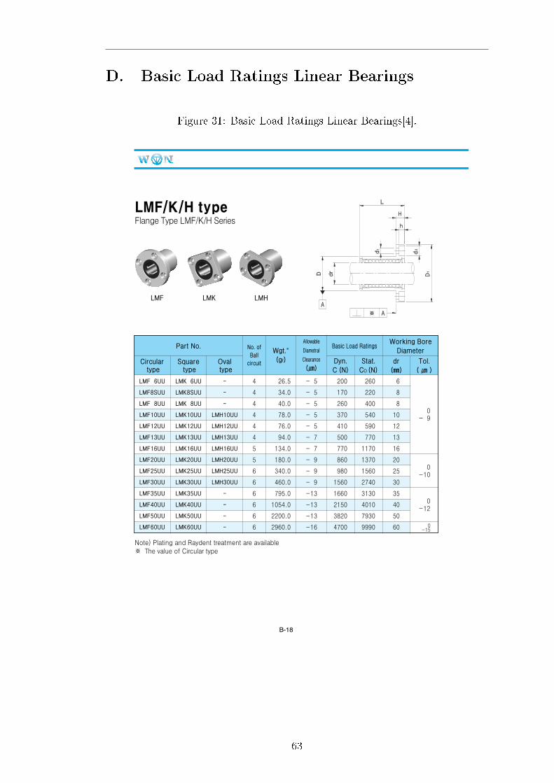
B-18
LMF/K/H typeFlange Type LMF/K/H Series
LMF LMK LMH
Note) Plating and Raydent treatment are available※ The value of Circular type
Circulartype
LMF 6UU
LMF8SUU
LMF 8UU
LMF10UU
LMF12UU
LMF13UU
LMF16UU
LMF20UU
LMF25UU
LMF30UU
LMF35UU
LMF40UU
LMF50UU
LMF60UU
Squaretype
LMK 6UU
LMK8SUU
LMK 8UU
LMK10UU
LMK12UU
LMK13UU
LMK16UU
LMK20UU
LMK25UU
LMK30UU
LMK35UU
LMK40UU
LMK50UU
LMK60UU
Ovaltype
-
-
-
LMH10UU
LMH12UU
LMH13UU
LMH16UU
LMH20UU
LMH25UU
LMH30UU
-
-
-
-
Part No. Basic Load RatingsWorking Bore
Diameter
4
4
4
4
4
4
5
5
6
6
6
6
6
6
No. ofBall
circuit
0200
0170
0260
0370
0410
0500
0770
0860
0980
1560
1660
2150
3820
4700
Dyn.C (N)
0260
0220
0400
0540
0590
0770
1170
1370
1560
2740
3130
4010
7930
9990
Stat.CO (N)
06
08
08
10
12
13
16
20
25
30
35
40
50
60
dr(㎜)
Tol.( ㎛ )
0026.5
0034.0
0040.0
0078.0
0076.0
0094.0
0134.0
0180.0
0340.0
0460.0
0795.0
1054.0
2200.0
2960.0
Wgt.※
(gf)
-05
-05
-05
-05
-05
-07
-07
-09
-09
-09
-13
-13
-13
-16
Allowable
Diametral
Clearance
(㎛)
-10-09
-10-10
-10-12
-10-15
02 B-리니어 볼부슁(22p.)3 2008.3.5 7:26 AM 페이지18 G4-1G (Mac 2) C-1800 1800DPI 150LPI T
D. Basic Load Ratings Linear Bearings
Figure 31: Basic Load Ratings Linear Bearings[4].
63
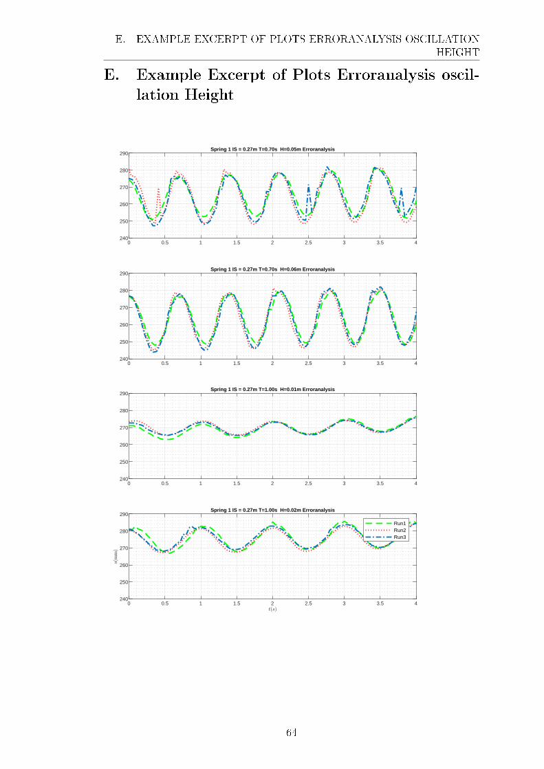
0 0.5 1 1.5 2 2.5 3 3.5 4240
250
260
270
280
290 Spring 1 IS = 0.27m T=1.00s H=0.02m Erroranalysis
Run1Run2Run3
0 0.5 1 1.5 2 2.5 3 3.5 4240
250
260
270
280
290 Spring 1 IS = 0.27m T=1.00s H=0.01m Erroranalysis
0 0.5 1 1.5 2 2.5 3 3.5 4240
250
260
270
280
290 Spring 1 IS = 0.27m T=0.70s H=0.06m Erroranalysis
0 0.5 1 1.5 2 2.5 3 3.5 4240
250
260
270
280
290 Spring 1 IS = 0.27m T=0.70s H=0.05m Erroranalysis
E. EXAMPLE EXCERPT OF PLOTS ERRORANALYSIS OSCILLATIONHEIGHT
E. Example Excerpt of Plots Erroranalysis oscil-
lation Height
64

F. ERRORANALYSIS OSZILLATION HEIGHT
F. Erroranalysis Oszillation Height
Table 7: Erroranalysis Oszillation Height
Oscillation height error Hoz,error [%] spring 1, IS = 0.27 m
H [mm]P [s] 0.70 1.00 1.25 1.50 1.75
10 36.585 7.843 3.158 − −
20 2.679 12.903 4.523 7.895 32.274
30 6.134 16.837 2.504 14.308 9.722
40 21.708 27.128 12.635 14.224 19.135
50 22.600 19.197 17.010 9.307 6.608
60 12.460 31.496 10.855 4.282 25.445
Oscillation height error Hoz,error [%] spring 1, IS = 0.21 m
H [mm]P [s] 0.70 1.00 1.25 1.50 1.75
10 39.669 4.225 15.190 − −
20 11.588 128.571 7.031 3.896 10.881
30 5.590 6.250 10.297 15.854 4.810
40 1.342 6.742 2.857 10.955 7.500
50 40.244 3.301 5.488 36.720 19.041
60 13.500 5.849 4.324 18.847 21.951
Oscillation height error Hoz,error [%] spring 1, IS = 0.15 m
H [mm]P [s] 0.70 1.00 1.25 1.50 1.75
10 178.378 14.286 11.413 − −
20 27.778 58.696 11.765 14.907 31.214
30 7.229 8.411 11.407 6.774 18.689
40 8.434 6.040 6.818 14.005 21.053
50 14.201 3.896 6.027 4.200 29.876
60 4.945 6.865 12.233 11.205 25.789
65

F. ERRORANALYSIS OSZILLATION HEIGHT
Oscillation height error Hoz,error [%] spring 1, IS = 0.09 m
H [mm]P [s] 0.70 1.00 1.25 1.50 1.75
10 20.000 45.652 95.455 − −
20 54.207 20.594 14.596 10.791 23.388
30 27.433 23.909 13.421 31.479 30.710
40 6.462 14.414 18.796 3.891 9.935
50 9.661 3.792 12.623 10.762 9.378
60 2.290 8.999 3.295 12.415 15.228
66

0 0.5 1 1.5 2 2.5 3 3.5 4
0.26
0.28
0.3
0.32
0.34 CP Spring 1 IS=0.27m T=0.70s H=0.01m Run=1
0 0.5 1 1.5 2 2.5 3 3.5 4
0.24
0.26
0.28
0.3
0 0.5 1 1.5 2 2.5 3 3.5 4
0.26
0.28
0.3
0.32
0.34 CP Spring 1 IS=0.27m T=0.70s H=0.02m Run=1
0 0.5 1 1.5 2 2.5 3 3.5 4
0.24
0.26
0.28
0.3
0 0.5 1 1.5 2 2.5 3 3.5 4
0.26
0.28
0.3
0.32
0.34 CP Spring 1 IS=0.27m T=0.70s H=0.03m Run=1
Gauge 1Gauge 2Gauge 3
0 0.5 1 1.5 2 2.5 3 3.5 4
0.24
0.26
0.28
0.3 Testobject CP
G. PLOTS OSCILLATION HEIGHT TESTOBJECT CIRCULAR PLATE
G. Plots Oscillation Height Testobject Circular
Plate
67

0 0.5 1 1.5 2 2.5 3 3.5 40.26
0.28
0.3
0.32
0.34
0.36 CP Spring 1 IS=0.27m T=0.70s H=0.04m Run=2
0 0.5 1 1.5 2 2.5 3 3.5 4
0.24
0.26
0.28
0.3
0 0.5 1 1.5 2 2.5 3 3.5 40.26
0.28
0.3
0.32
0.34
0.36 CP Spring 1 IS=0.27m T=0.70s H=0.05m Run=2
0 0.5 1 1.5 2 2.5 3 3.5 4
0.24
0.26
0.28
0.3
0 0.5 1 1.5 2 2.5 3 3.5 40.26
0.28
0.3
0.32
0.34
0.36 CP Spring 1 IS=0.27m T=0.70s H=0.06m Run=3
Gauge 1Gauge 2Gauge 3
0 0.5 1 1.5 2 2.5 3 3.5 4
0.24
0.26
0.28
0.3 Testobject CP
G. PLOTS OSCILLATION HEIGHT TESTOBJECT CIRCULAR PLATE
68

0 0.5 1 1.5 2 2.5 3 3.5 40.26
0.28
0.3
0.32
0.34
0.36 CP Spring 1 IS=0.27m T=1.00s H=0.01m Run=2
0 0.5 1 1.5 2 2.5 3 3.5 4
0.24
0.26
0.28
0.3
0 0.5 1 1.5 2 2.5 3 3.5 40.26
0.28
0.3
0.32
0.34
0.36 CP Spring 1 IS=0.27m T=1.00s H=0.02m Run=1
0 0.5 1 1.5 2 2.5 3 3.5 4
0.24
0.26
0.28
0.3
0 0.5 1 1.5 2 2.5 3 3.5 40.26
0.28
0.3
0.32
0.34
0.36 CP Spring 1 IS=0.27m T=1.00s H=0.03m Run=1
Gauge 1Gauge 2Gauge 3
0 0.5 1 1.5 2 2.5 3 3.5 4
0.24
0.26
0.28
0.3 Testobject CP
G. PLOTS OSCILLATION HEIGHT TESTOBJECT CIRCULAR PLATE
69
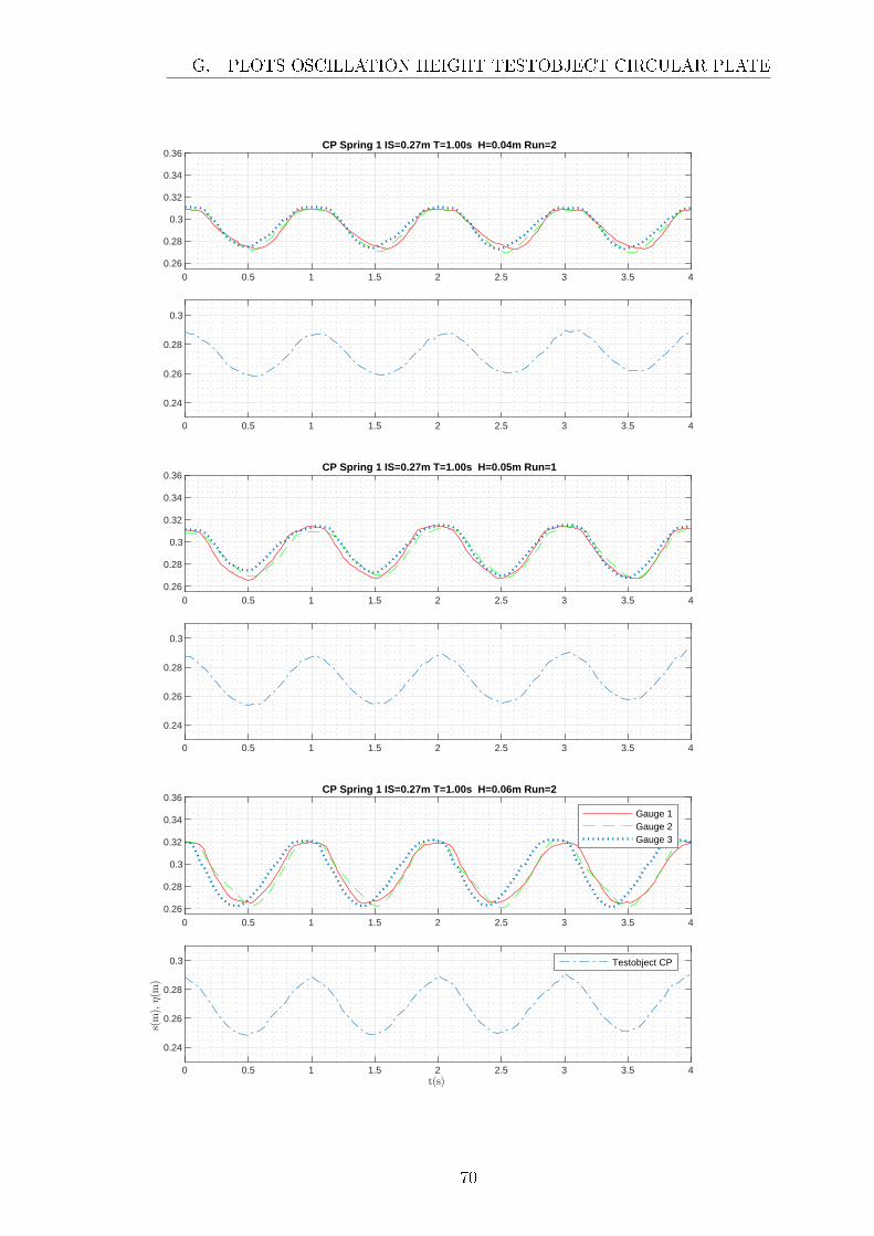
0 0.5 1 1.5 2 2.5 3 3.5 40.26
0.28
0.3
0.32
0.34
0.36 CP Spring 1 IS=0.27m T=1.00s H=0.04m Run=2
0 0.5 1 1.5 2 2.5 3 3.5 4
0.24
0.26
0.28
0.3
0 0.5 1 1.5 2 2.5 3 3.5 40.26
0.28
0.3
0.32
0.34
0.36 CP Spring 1 IS=0.27m T=1.00s H=0.05m Run=1
0 0.5 1 1.5 2 2.5 3 3.5 4
0.24
0.26
0.28
0.3
0 0.5 1 1.5 2 2.5 3 3.5 40.26
0.28
0.3
0.32
0.34
0.36 CP Spring 1 IS=0.27m T=1.00s H=0.06m Run=2
Gauge 1Gauge 2Gauge 3
0 0.5 1 1.5 2 2.5 3 3.5 4
0.24
0.26
0.28
0.3 Testobject CP
G. PLOTS OSCILLATION HEIGHT TESTOBJECT CIRCULAR PLATE
70

0 0.5 1 1.5 2 2.5 3 3.5 40.26
0.28
0.3
0.32
0.34
0.36 CP Spring 1 IS=0.27m T=1.25s H=0.01m Run=1
0 0.5 1 1.5 2 2.5 3 3.5 4
0.24
0.26
0.28
0.3
0 0.5 1 1.5 2 2.5 3 3.5 40.26
0.28
0.3
0.32
0.34
0.36 CP Spring 1 IS=0.27m T=1.25s H=0.02m Run=2
0 0.5 1 1.5 2 2.5 3 3.5 4
0.24
0.26
0.28
0.3
0 0.5 1 1.5 2 2.5 3 3.5 40.26
0.28
0.3
0.32
0.34
0.36 CP Spring 1 IS=0.27m T=1.25s H=0.03m Run=1
Gauge 1Gauge 2Gauge 3
0 0.5 1 1.5 2 2.5 3 3.5 4
0.24
0.26
0.28
0.3 Testobject CP
G. PLOTS OSCILLATION HEIGHT TESTOBJECT CIRCULAR PLATE
71

0 0.5 1 1.5 2 2.5 3 3.5 40.26
0.28
0.3
0.32
0.34
0.36 CP Spring 1 IS=0.27m T=1.25s H=0.04m Run=1
0 0.5 1 1.5 2 2.5 3 3.5 4
0.24
0.26
0.28
0.3
0 0.5 1 1.5 2 2.5 3 3.5 40.26
0.28
0.3
0.32
0.34
0.36 CP Spring 1 IS=0.27m T=1.25s H=0.05m Run=2
0 0.5 1 1.5 2 2.5 3 3.5 4
0.24
0.26
0.28
0.3
0 0.5 1 1.5 2 2.5 3 3.5 40.26
0.28
0.3
0.32
0.34
0.36 CP Spring 1 IS=0.27m T=1.25s H=0.06m Run=3
Gauge 1Gauge 2Gauge 3
0 0.5 1 1.5 2 2.5 3 3.5 4
0.24
0.26
0.28
0.3 Testobject CP
G. PLOTS OSCILLATION HEIGHT TESTOBJECT CIRCULAR PLATE
72

0 0.5 1 1.5 2 2.5 3 3.5 40.26
0.28
0.3
0.32
0.34
0.36 CP Spring 1 IS=0.27m T=1.50s H=0.02m Run=1
0 0.5 1 1.5 2 2.5 3 3.5 4
0.24
0.26
0.28
0.3
0 0.5 1 1.5 2 2.5 3 3.5 40.26
0.28
0.3
0.32
0.34
0.36 CP Spring 1 IS=0.27m T=1.50s H=0.03m Run=1
0 0.5 1 1.5 2 2.5 3 3.5 4
0.24
0.26
0.28
0.3
0 0.5 1 1.5 2 2.5 3 3.5 40.26
0.28
0.3
0.32
0.34
0.36 CP Spring 1 IS=0.27m T=1.50s H=0.04m Run=3
Gauge 1Gauge 2Gauge 3
0 0.5 1 1.5 2 2.5 3 3.5 4
0.24
0.26
0.28
0.3 Testobject CP
G. PLOTS OSCILLATION HEIGHT TESTOBJECT CIRCULAR PLATE
73

0 0.5 1 1.5 2 2.5 3 3.5 40.26
0.28
0.3
0.32
0.34
0.36 CP Spring 1 IS=0.27m T=1.50s H=0.05m Run=3
0 0.5 1 1.5 2 2.5 3 3.5 4
0.24
0.26
0.28
0.3
0 0.5 1 1.5 2 2.5 3 3.5 40.26
0.28
0.3
0.32
0.34
0.36 CP Spring 1 IS=0.27m T=1.50s H=0.06m Run=1
0 0.5 1 1.5 2 2.5 3 3.5 4
0.24
0.26
0.28
0.3
0 0.5 1 1.5 2 2.5 3 3.5 40.26
0.28
0.3
0.32
0.34
0.36 CP Spring 1 IS=0.27m T=1.75s H=0.02m Run=3
Gauge 1Gauge 2Gauge 3
0 0.5 1 1.5 2 2.5 3 3.5 4
0.24
0.26
0.28
0.3 Testobject CP
G. PLOTS OSCILLATION HEIGHT TESTOBJECT CIRCULAR PLATE
74

0 0.5 1 1.5 2 2.5 3 3.5 40.26
0.28
0.3
0.32
0.34
0.36 CP Spring 1 IS=0.27m T=1.75s H=0.03m Run=1
0 0.5 1 1.5 2 2.5 3 3.5 4
0.24
0.26
0.28
0.3
0 0.5 1 1.5 2 2.5 3 3.5 40.26
0.28
0.3
0.32
0.34
0.36 CP Spring 1 IS=0.27m T=1.75s H=0.04m Run=1
0 0.5 1 1.5 2 2.5 3 3.5 4
0.24
0.26
0.28
0.3
0 0.5 1 1.5 2 2.5 3 3.5 40.26
0.28
0.3
0.32
0.34
0.36 CP Spring 1 IS=0.27m T=1.75s H=0.05m Run=2
Gauge 1Gauge 2Gauge 3
0 0.5 1 1.5 2 2.5 3 3.5 4
0.24
0.26
0.28
0.3 Testobject CP
G. PLOTS OSCILLATION HEIGHT TESTOBJECT CIRCULAR PLATE
75
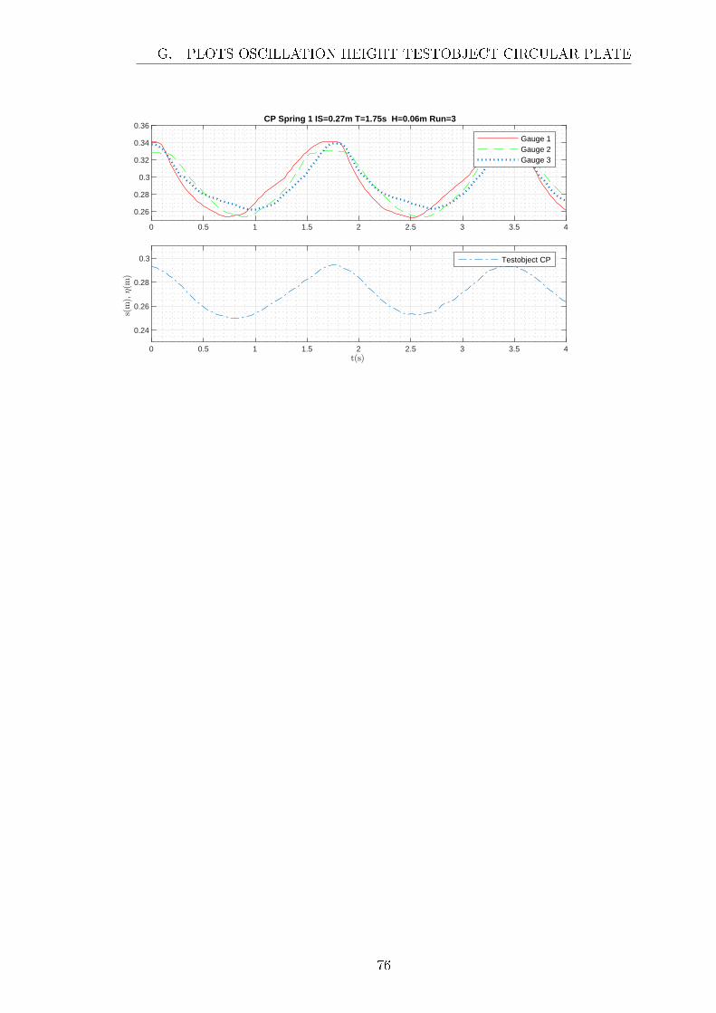
0 0.5 1 1.5 2 2.5 3 3.5 4
0.26
0.28
0.3
0.32
0.34
0.36 CP Spring 1 IS=0.27m T=1.75s H=0.06m Run=3
Gauge 1Gauge 2Gauge 3
0 0.5 1 1.5 2 2.5 3 3.5 4
0.24
0.26
0.28
0.3 Testobject CP
G. PLOTS OSCILLATION HEIGHT TESTOBJECT CIRCULAR PLATE
76

0 0.5 1 1.5 2 2.5 3 3.5 4
0.26
0.28
0.3
0.32
0.34 CP Spring 1 IS=0.21m T=0.70s H=0.01m Run=1
0 0.5 1 1.5 2 2.5 3 3.5 40.18
0.2
0.22
0.24
0.26
0 0.5 1 1.5 2 2.5 3 3.5 4
0.26
0.28
0.3
0.32
0.34 CP Spring 1 IS=0.21m T=0.70s H=0.02m Run=1
0 0.5 1 1.5 2 2.5 3 3.5 40.18
0.2
0.22
0.24
0.26
0 0.5 1 1.5 2 2.5 3 3.5 4
0.26
0.28
0.3
0.32
0.34 CP Spring 1 IS=0.21m T=0.70s H=0.03m Run=3
Gauge 1Gauge 2Gauge 3
0 0.5 1 1.5 2 2.5 3 3.5 40.18
0.2
0.22
0.24
0.26
Testobject CP
G. PLOTS OSCILLATION HEIGHT TESTOBJECT CIRCULAR PLATE
77

0 0.5 1 1.5 2 2.5 3 3.5 4
0.26
0.28
0.3
0.32
0.34
0.36 CP Spring 2 IS=0.21m T=1.25s H=0.04m Run=2
0 0.5 1 1.5 2 2.5 3 3.5 40.18
0.2
0.22
0.24
0.26
0 0.5 1 1.5 2 2.5 3 3.5 4
0.26
0.28
0.3
0.32
0.34
0.36 CP Spring 2 IS=0.21m T=1.25s H=0.05m Run=1
0 0.5 1 1.5 2 2.5 3 3.5 40.18
0.2
0.22
0.24
0.26
0 0.5 1 1.5 2 2.5 3 3.5 4
0.26
0.28
0.3
0.32
0.34
0.36 CP Spring 2 IS=0.21m T=1.25s H=0.06m Run=1
Gauge 1Gauge 2
0 0.5 1 1.5 2 2.5 3 3.5 40.18
0.2
0.22
0.24
0.26
Testobject CP
G. PLOTS OSCILLATION HEIGHT TESTOBJECT CIRCULAR PLATE
78
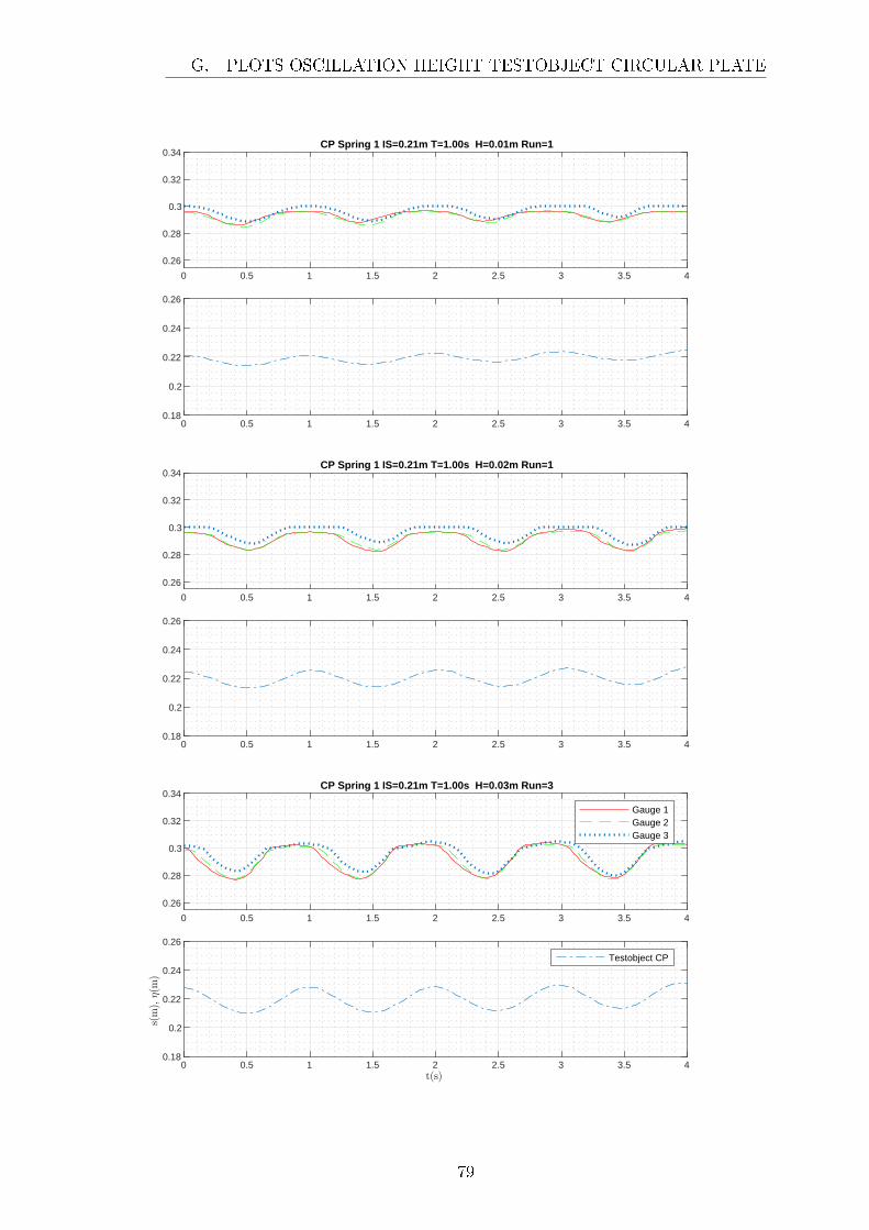
0 0.5 1 1.5 2 2.5 3 3.5 4
0.26
0.28
0.3
0.32
0.34 CP Spring 1 IS=0.21m T=1.00s H=0.01m Run=1
0 0.5 1 1.5 2 2.5 3 3.5 40.18
0.2
0.22
0.24
0.26
0 0.5 1 1.5 2 2.5 3 3.5 4
0.26
0.28
0.3
0.32
0.34 CP Spring 1 IS=0.21m T=1.00s H=0.02m Run=1
0 0.5 1 1.5 2 2.5 3 3.5 40.18
0.2
0.22
0.24
0.26
0 0.5 1 1.5 2 2.5 3 3.5 4
0.26
0.28
0.3
0.32
0.34 CP Spring 1 IS=0.21m T=1.00s H=0.03m Run=3
Gauge 1Gauge 2Gauge 3
0 0.5 1 1.5 2 2.5 3 3.5 40.18
0.2
0.22
0.24
0.26
Testobject CP
G. PLOTS OSCILLATION HEIGHT TESTOBJECT CIRCULAR PLATE
79

0 0.5 1 1.5 2 2.5 3 3.5 4
0.26
0.28
0.3
0.32
0.34 CP Spring 1 IS=0.21m T=1.00s H=0.04m Run=1
0 0.5 1 1.5 2 2.5 3 3.5 40.18
0.2
0.22
0.24
0.26
0 0.5 1 1.5 2 2.5 3 3.5 4
0.26
0.28
0.3
0.32
0.34 CP Spring 1 IS=0.21m T=1.00s H=0.05m Run=1
0 0.5 1 1.5 2 2.5 3 3.5 40.18
0.2
0.22
0.24
0.26
0 0.5 1 1.5 2 2.5 3 3.5 4
0.26
0.28
0.3
0.32
0.34 CP Spring 1 IS=0.21m T=1.00s H=0.06m Run=3
Gauge 1Gauge 2Gauge 3
0 0.5 1 1.5 2 2.5 3 3.5 40.18
0.2
0.22
0.24
0.26
Testobject CP
G. PLOTS OSCILLATION HEIGHT TESTOBJECT CIRCULAR PLATE
80

0 0.5 1 1.5 2 2.5 3 3.5 4
0.26
0.28
0.3
0.32
0.34 CP Spring 1 IS=0.21m T=1.25s H=0.01m Run=1
0 0.5 1 1.5 2 2.5 3 3.5 40.18
0.2
0.22
0.24
0.26
0 0.5 1 1.5 2 2.5 3 3.5 4
0.26
0.28
0.3
0.32
0.34 CP Spring 1 IS=0.21m T=1.25s H=0.02m Run=1
0 0.5 1 1.5 2 2.5 3 3.5 40.18
0.2
0.22
0.24
0.26
0 0.5 1 1.5 2 2.5 3 3.5 4
0.26
0.28
0.3
0.32
0.34 CP Spring 1 IS=0.21m T=1.25s H=0.03m Run=2
Gauge 1Gauge 2Gauge 3
0 0.5 1 1.5 2 2.5 3 3.5 40.18
0.2
0.22
0.24
0.26
Testobject CP
G. PLOTS OSCILLATION HEIGHT TESTOBJECT CIRCULAR PLATE
81

0 0.5 1 1.5 2 2.5 3 3.5 40.15
0.2
0.25
0.3
0.35
0.4 CP Spring 1 IS=0.21m T=1.25s H=0.04m Run=1
0 0.5 1 1.5 2 2.5 3 3.5 40.18
0.2
0.22
0.24
0.26
0 0.5 1 1.5 2 2.5 3 3.5 40.15
0.2
0.25
0.3
0.35
0.4 CP Spring 1 IS=0.21m T=1.25s H=0.05m Run=1
0 0.5 1 1.5 2 2.5 3 3.5 40.18
0.2
0.22
0.24
0.26
0 0.5 1 1.5 2 2.5 3 3.5 40.15
0.2
0.25
0.3
0.35
0.4 CP Spring 1 IS=0.21m T=1.25s H=0.06m Run=1
Gauge 1Gauge 2Gauge 3
0 0.5 1 1.5 2 2.5 3 3.5 40.18
0.2
0.22
0.24
0.26
Testobject CP
G. PLOTS OSCILLATION HEIGHT TESTOBJECT CIRCULAR PLATE
82

0 0.5 1 1.5 2 2.5 3 3.5 4
0.26
0.28
0.3
0.32
0.34 CP Spring 1 IS=0.21m T=1.50s H=0.02m Run=1
0 0.5 1 1.5 2 2.5 3 3.5 40.18
0.2
0.22
0.24
0.26
0 0.5 1 1.5 2 2.5 3 3.5 4
0.26
0.28
0.3
0.32
0.34 CP Spring 1 IS=0.21m T=1.50s H=0.03m Run=1
0 0.5 1 1.5 2 2.5 3 3.5 40.18
0.2
0.22
0.24
0.26
0 0.5 1 1.5 2 2.5 3 3.5 4
0.26
0.28
0.3
0.32
0.34 CP Spring 1 IS=0.21m T=1.50s H=0.04m Run=1
Gauge 1
0 0.5 1 1.5 2 2.5 3 3.5 40.18
0.2
0.22
0.24
0.26
Testobject CP
G. PLOTS OSCILLATION HEIGHT TESTOBJECT CIRCULAR PLATE
83

0 0.5 1 1.5 2 2.5 3 3.5 4
0.26
0.28
0.3
0.32
0.34 CP Spring 1 IS=0.21m T=1.50s H=0.05m Run=1
0 0.5 1 1.5 2 2.5 3 3.5 40.18
0.2
0.22
0.24
0.26
0 0.5 1 1.5 2 2.5 3 3.5 4
0.26
0.28
0.3
0.32
0.34 CP Spring 1 IS=0.21m T=1.50s H=0.06m Run=1
0 0.5 1 1.5 2 2.5 3 3.5 40.18
0.2
0.22
0.24
0.26
0 0.5 1 1.5 2 2.5 3 3.5 4
0.26
0.28
0.3
0.32
0.34 CP Spring 1 IS=0.21m T=1.75s H=0.02m Run=1
Gauge 1
0 0.5 1 1.5 2 2.5 3 3.5 40.18
0.2
0.22
0.24
0.26
Testobject CP
G. PLOTS OSCILLATION HEIGHT TESTOBJECT CIRCULAR PLATE
84

0 0.5 1 1.5 2 2.5 3 3.5 4
0.26
0.28
0.3
0.32
0.34 CP Spring 1 IS=0.21m T=1.75s H=0.03m Run=1
0 0.5 1 1.5 2 2.5 3 3.5 40.18
0.2
0.22
0.24
0.26
0 0.5 1 1.5 2 2.5 3 3.5 4
0.26
0.28
0.3
0.32
0.34 CP Spring 1 IS=0.21m T=1.75s H=0.04m Run=1
0 0.5 1 1.5 2 2.5 3 3.5 40.18
0.2
0.22
0.24
0.26
0 0.5 1 1.5 2 2.5 3 3.5 4
0.26
0.28
0.3
0.32
0.34 CP Spring 1 IS=0.21m T=1.75s H=0.05m Run=1
Gauge 1
0 0.5 1 1.5 2 2.5 3 3.5 40.18
0.2
0.22
0.24
0.26
Testobject CP
G. PLOTS OSCILLATION HEIGHT TESTOBJECT CIRCULAR PLATE
85
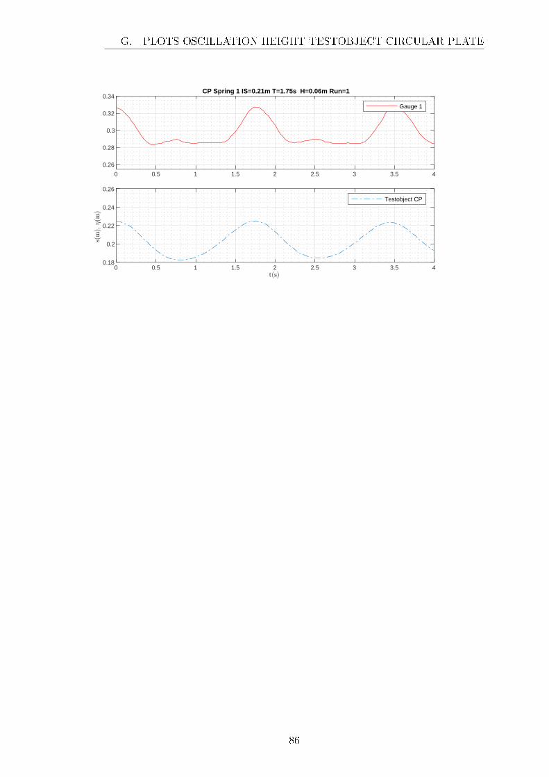
0 0.5 1 1.5 2 2.5 3 3.5 4
0.26
0.28
0.3
0.32
0.34 CP Spring 1 IS=0.21m T=1.75s H=0.06m Run=1
Gauge 1
0 0.5 1 1.5 2 2.5 3 3.5 40.18
0.2
0.22
0.24
0.26
Testobject CP
G. PLOTS OSCILLATION HEIGHT TESTOBJECT CIRCULAR PLATE
86
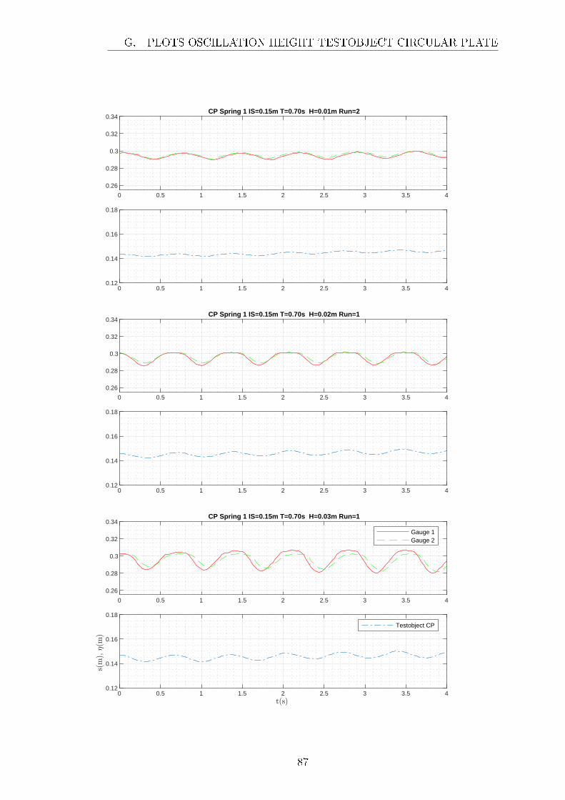
0 0.5 1 1.5 2 2.5 3 3.5 4
0.26
0.28
0.3
0.32
0.34 CP Spring 1 IS=0.15m T=0.70s H=0.01m Run=2
0 0.5 1 1.5 2 2.5 3 3.5 40.12
0.14
0.16
0.18
0 0.5 1 1.5 2 2.5 3 3.5 4
0.26
0.28
0.3
0.32
0.34 CP Spring 1 IS=0.15m T=0.70s H=0.02m Run=1
0 0.5 1 1.5 2 2.5 3 3.5 40.12
0.14
0.16
0.18
0 0.5 1 1.5 2 2.5 3 3.5 4
0.26
0.28
0.3
0.32
0.34 CP Spring 1 IS=0.15m T=0.70s H=0.03m Run=1
Gauge 1Gauge 2
0 0.5 1 1.5 2 2.5 3 3.5 40.12
0.14
0.16
0.18
Testobject CP
G. PLOTS OSCILLATION HEIGHT TESTOBJECT CIRCULAR PLATE
87
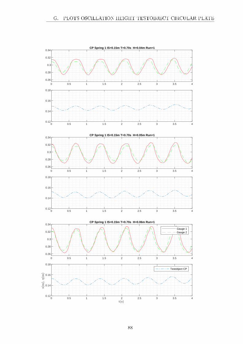
0 0.5 1 1.5 2 2.5 3 3.5 4
0.26
0.28
0.3
0.32
0.34 CP Spring 1 IS=0.15m T=0.70s H=0.04m Run=1
0 0.5 1 1.5 2 2.5 3 3.5 40.12
0.14
0.16
0.18
0 0.5 1 1.5 2 2.5 3 3.5 4
0.26
0.28
0.3
0.32
0.34 CP Spring 1 IS=0.15m T=0.70s H=0.05m Run=1
0 0.5 1 1.5 2 2.5 3 3.5 40.12
0.14
0.16
0.18
0 0.5 1 1.5 2 2.5 3 3.5 4
0.26
0.28
0.3
0.32
0.34 CP Spring 1 IS=0.15m T=0.70s H=0.06m Run=1
Gauge 1Gauge 2
0 0.5 1 1.5 2 2.5 3 3.5 40.12
0.14
0.16
0.18
Testobject CP
G. PLOTS OSCILLATION HEIGHT TESTOBJECT CIRCULAR PLATE
88

0 0.5 1 1.5 2 2.5 3 3.5 4
0.26
0.28
0.3
0.32
0.34 CP Spring 1 IS=0.15m T=1.00s H=0.01m Run=1
0 0.5 1 1.5 2 2.5 3 3.5 40.12
0.14
0.16
0.18
0 0.5 1 1.5 2 2.5 3 3.5 4
0.26
0.28
0.3
0.32
0.34 CP Spring 1 IS=0.15m T=1.00s H=0.02m Run=1
0 0.5 1 1.5 2 2.5 3 3.5 40.12
0.14
0.16
0.18
0 0.5 1 1.5 2 2.5 3 3.5 4
0.26
0.28
0.3
0.32
0.34 CP Spring 1 IS=0.15m T=1.00s H=0.03m Run=1
Gauge 1Gauge 2
0 0.5 1 1.5 2 2.5 3 3.5 40.12
0.14
0.16
0.18
Testobject CP
G. PLOTS OSCILLATION HEIGHT TESTOBJECT CIRCULAR PLATE
89

0 0.5 1 1.5 2 2.5 3 3.5 4
0.26
0.28
0.3
0.32
0.34 CP Spring 1 IS=0.15m T=1.00s H=0.04m Run=1
0 0.5 1 1.5 2 2.5 3 3.5 40.12
0.14
0.16
0.18
0 0.5 1 1.5 2 2.5 3 3.5 4
0.26
0.28
0.3
0.32
0.34 CP Spring 1 IS=0.15m T=1.00s H=0.05m Run=1
0 0.5 1 1.5 2 2.5 3 3.5 40.12
0.14
0.16
0.18
0 0.5 1 1.5 2 2.5 3 3.5 4
0.26
0.28
0.3
0.32
0.34 CP Spring 1 IS=0.15m T=1.00s H=0.06m Run=1
Gauge 1Gauge 2
0 0.5 1 1.5 2 2.5 3 3.5 40.12
0.14
0.16
0.18
Testobject CP
G. PLOTS OSCILLATION HEIGHT TESTOBJECT CIRCULAR PLATE
90
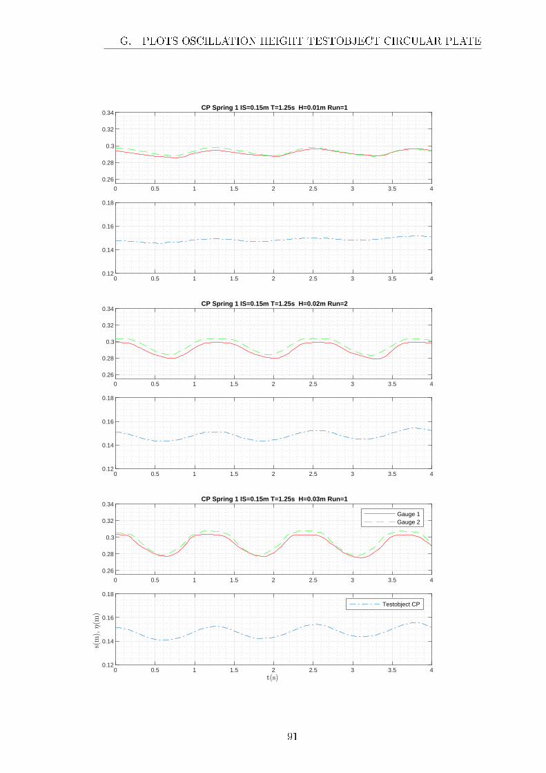
0 0.5 1 1.5 2 2.5 3 3.5 4
0.26
0.28
0.3
0.32
0.34 CP Spring 1 IS=0.15m T=1.25s H=0.01m Run=1
0 0.5 1 1.5 2 2.5 3 3.5 40.12
0.14
0.16
0.18
0 0.5 1 1.5 2 2.5 3 3.5 4
0.26
0.28
0.3
0.32
0.34 CP Spring 1 IS=0.15m T=1.25s H=0.02m Run=2
0 0.5 1 1.5 2 2.5 3 3.5 40.12
0.14
0.16
0.18
0 0.5 1 1.5 2 2.5 3 3.5 4
0.26
0.28
0.3
0.32
0.34 CP Spring 1 IS=0.15m T=1.25s H=0.03m Run=1
Gauge 1Gauge 2
0 0.5 1 1.5 2 2.5 3 3.5 40.12
0.14
0.16
0.18
Testobject CP
G. PLOTS OSCILLATION HEIGHT TESTOBJECT CIRCULAR PLATE
91
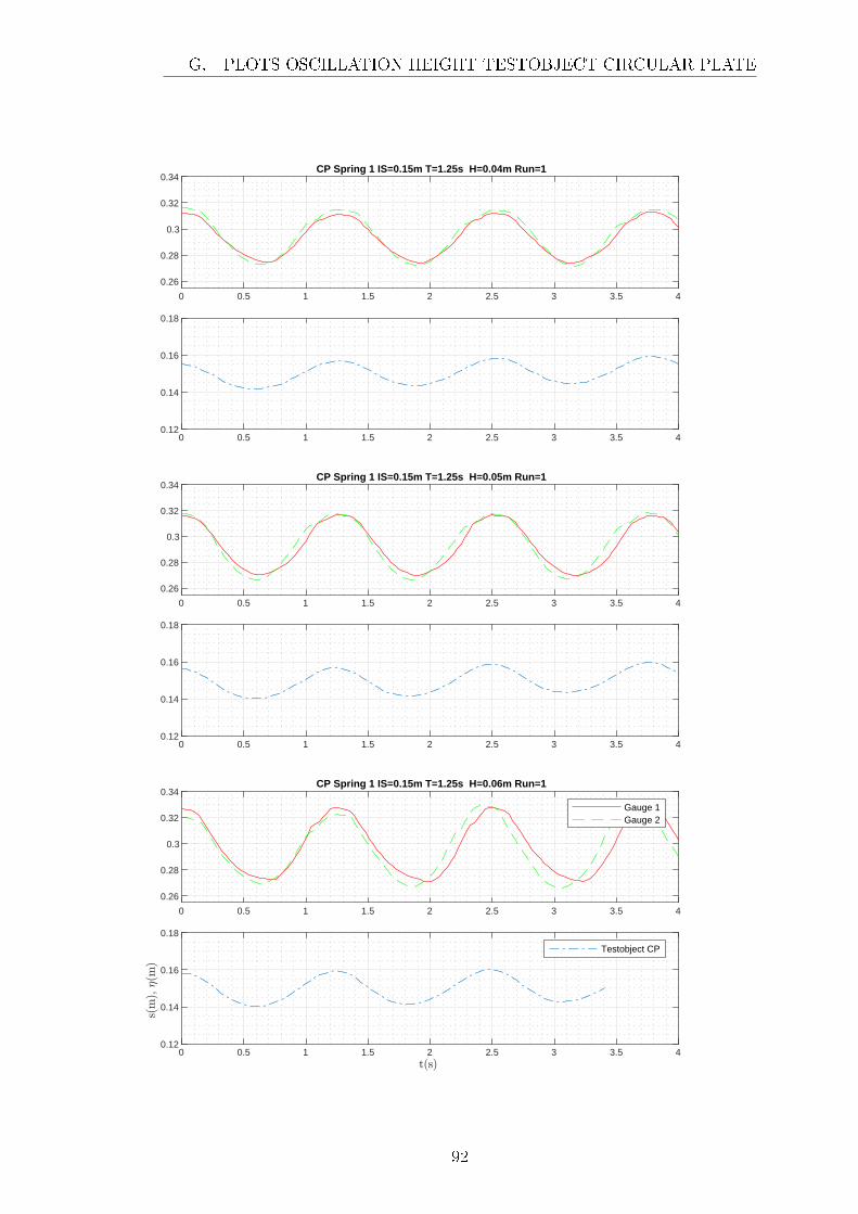
0 0.5 1 1.5 2 2.5 3 3.5 4
0.26
0.28
0.3
0.32
0.34 CP Spring 1 IS=0.15m T=1.25s H=0.04m Run=1
0 0.5 1 1.5 2 2.5 3 3.5 40.12
0.14
0.16
0.18
0 0.5 1 1.5 2 2.5 3 3.5 4
0.26
0.28
0.3
0.32
0.34 CP Spring 1 IS=0.15m T=1.25s H=0.05m Run=1
0 0.5 1 1.5 2 2.5 3 3.5 40.12
0.14
0.16
0.18
0 0.5 1 1.5 2 2.5 3 3.5 4
0.26
0.28
0.3
0.32
0.34 CP Spring 1 IS=0.15m T=1.25s H=0.06m Run=1
Gauge 1Gauge 2
0 0.5 1 1.5 2 2.5 3 3.5 40.12
0.14
0.16
0.18
Testobject CP
G. PLOTS OSCILLATION HEIGHT TESTOBJECT CIRCULAR PLATE
92

0 0.5 1 1.5 2 2.5 3 3.5 4
0.26
0.28
0.3
0.32
0.34 CP Spring 1 IS=0.15m T=1.50s H=0.02m Run=1
0 0.5 1 1.5 2 2.5 3 3.5 40.12
0.14
0.16
0.18
0 0.5 1 1.5 2 2.5 3 3.5 4
0.26
0.28
0.3
0.32
0.34 CP Spring 1 IS=0.15m T=1.50s H=0.03m Run=1
0 0.5 1 1.5 2 2.5 3 3.5 40.12
0.14
0.16
0.18
0 0.5 1 1.5 2 2.5 3 3.5 4
0.26
0.28
0.3
0.32
0.34 CP Spring 1 IS=0.15m T=1.50s H=0.04m Run=1
Gauge 1Gauge 2
0 0.5 1 1.5 2 2.5 3 3.5 40.12
0.14
0.16
0.18
Testobject CP
G. PLOTS OSCILLATION HEIGHT TESTOBJECT CIRCULAR PLATE
93

0 0.5 1 1.5 2 2.5 3 3.5 4
0.26
0.28
0.3
0.32
0.34 CP Spring 1 IS=0.15m T=1.50s H=0.05m Run=1
0 0.5 1 1.5 2 2.5 3 3.5 40.12
0.14
0.16
0.18
0 0.5 1 1.5 2 2.5 3 3.5 4
0.26
0.28
0.3
0.32
0.34 CP Spring 1 IS=0.15m T=1.50s H=0.06m Run=1
0 0.5 1 1.5 2 2.5 3 3.5 40.12
0.14
0.16
0.18
0 0.5 1 1.5 2 2.5 3 3.5 4
0.26
0.28
0.3
0.32
0.34 CP Spring 1 IS=0.15m T=1.75s H=0.02m Run=3
Gauge 1Gauge 2
0 0.5 1 1.5 2 2.5 3 3.5 40.12
0.14
0.16
0.18
Testobject CP
G. PLOTS OSCILLATION HEIGHT TESTOBJECT CIRCULAR PLATE
94

0 0.5 1 1.5 2 2.5 3 3.5 4
0.26
0.28
0.3
0.32
0.34 CP Spring 1 IS=0.15m T=1.75s H=0.03m Run=1
0 0.5 1 1.5 2 2.5 3 3.5 40.12
0.14
0.16
0.18
0 0.5 1 1.5 2 2.5 3 3.5 4
0.26
0.28
0.3
0.32
0.34 CP Spring 1 IS=0.15m T=1.75s H=0.04m Run=1
0 0.5 1 1.5 2 2.5 3 3.5 40.12
0.14
0.16
0.18
0 0.5 1 1.5 2 2.5 3 3.5 4
0.26
0.28
0.3
0.32
0.34 CP Spring 1 IS=0.15m T=1.75s H=0.05m Run=1
Gauge 1Gauge 2
0 0.5 1 1.5 2 2.5 3 3.5 40.12
0.14
0.16
0.18
Testobject CP
G. PLOTS OSCILLATION HEIGHT TESTOBJECT CIRCULAR PLATE
95

0 0.5 1 1.5 2 2.5 3 3.5 4
0.26
0.28
0.3
0.32
0.34
0.36 CP Spring 1 IS=0.15m T=1.75s H=0.06m Run=1
Gauge 1Gauge 2
0 0.5 1 1.5 2 2.5 3 3.5 40.12
0.14
0.16
0.18
Testobject CP
G. PLOTS OSCILLATION HEIGHT TESTOBJECT CIRCULAR PLATE
96
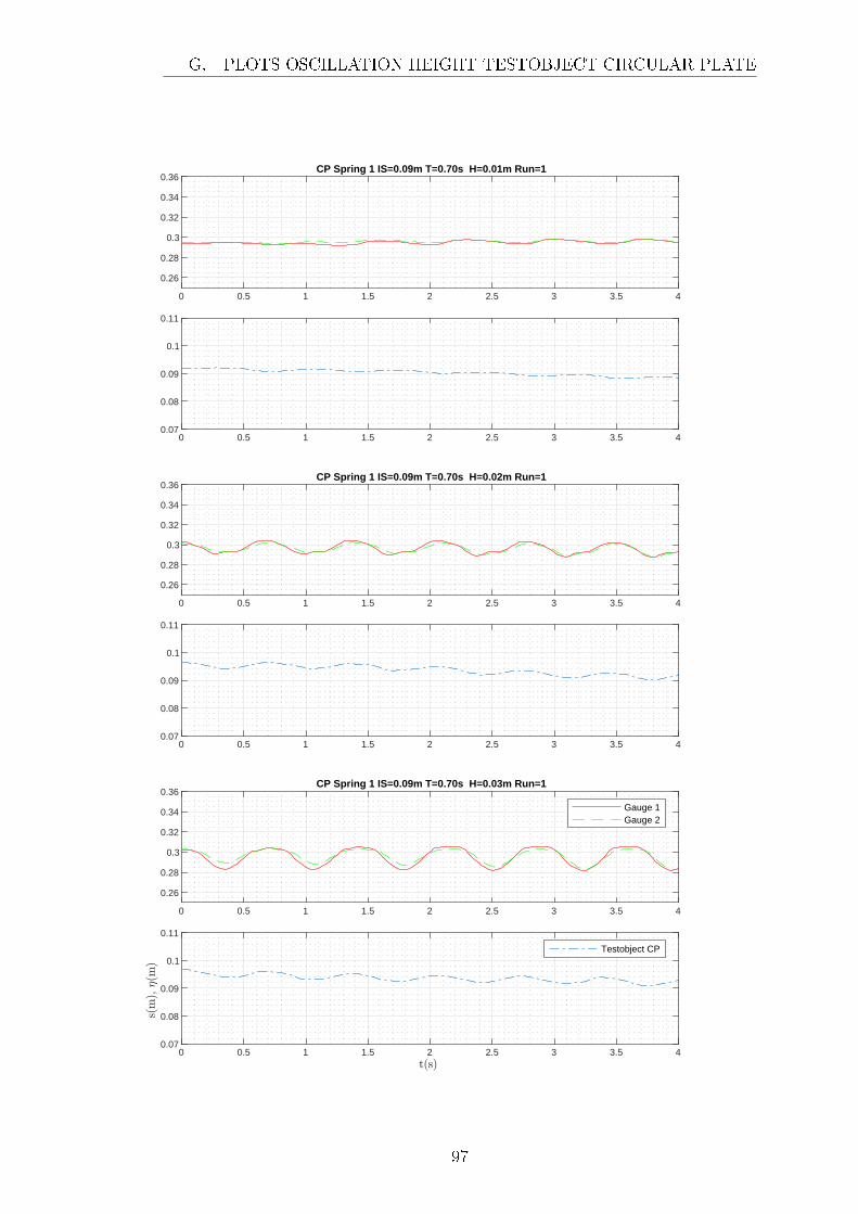
0 0.5 1 1.5 2 2.5 3 3.5 4
0.26
0.28
0.3
0.32
0.34
0.36 CP Spring 1 IS=0.09m T=0.70s H=0.01m Run=1
0 0.5 1 1.5 2 2.5 3 3.5 40.07
0.08
0.09
0.1
0.11
0 0.5 1 1.5 2 2.5 3 3.5 4
0.26
0.28
0.3
0.32
0.34
0.36 CP Spring 1 IS=0.09m T=0.70s H=0.02m Run=1
0 0.5 1 1.5 2 2.5 3 3.5 40.07
0.08
0.09
0.1
0.11
0 0.5 1 1.5 2 2.5 3 3.5 4
0.26
0.28
0.3
0.32
0.34
0.36 CP Spring 1 IS=0.09m T=0.70s H=0.03m Run=1
Gauge 1Gauge 2
0 0.5 1 1.5 2 2.5 3 3.5 40.07
0.08
0.09
0.1
0.11
Testobject CP
G. PLOTS OSCILLATION HEIGHT TESTOBJECT CIRCULAR PLATE
97

0 0.5 1 1.5 2 2.5 3 3.5 4
0.26
0.28
0.3
0.32
0.34
0.36 CP Spring 1 IS=0.09m T=0.70s H=0.04m Run=1
0 0.5 1 1.5 2 2.5 3 3.5 40.07
0.08
0.09
0.1
0.11
0 0.5 1 1.5 2 2.5 3 3.5 4
0.26
0.28
0.3
0.32
0.34
0.36 CP Spring 1 IS=0.09m T=0.70s H=0.05m Run=1
0 0.5 1 1.5 2 2.5 3 3.5 40.07
0.08
0.09
0.1
0.11
0 0.5 1 1.5 2 2.5 3 3.5 4
0.26
0.28
0.3
0.32
0.34
0.36 CP Spring 1 IS=0.09m T=0.70s H=0.06m Run=1
Gauge 1Gauge 2
0 0.5 1 1.5 2 2.5 3 3.5 40.07
0.08
0.09
0.1
0.11
Testobject CP
G. PLOTS OSCILLATION HEIGHT TESTOBJECT CIRCULAR PLATE
98

0 0.5 1 1.5 2 2.5 3 3.5 4
0.26
0.28
0.3
0.32
0.34
0.36 CP Spring 1 IS=0.09m T=1.00s H=0.01m Run=1
0 0.5 1 1.5 2 2.5 3 3.5 40.07
0.08
0.09
0.1
0.11
0 0.5 1 1.5 2 2.5 3 3.5 4
0.26
0.28
0.3
0.32
0.34
0.36 CP Spring 1 IS=0.09m T=1.00s H=0.02m Run=1
0 0.5 1 1.5 2 2.5 3 3.5 40.07
0.08
0.09
0.1
0.11
0 0.5 1 1.5 2 2.5 3 3.5 4
0.26
0.28
0.3
0.32
0.34
0.36 CP Spring 1 IS=0.09m T=1.00s H=0.03m Run=1
Gauge 1Gauge 2
0 0.5 1 1.5 2 2.5 3 3.5 40.07
0.08
0.09
0.1
0.11
Testobject CP
G. PLOTS OSCILLATION HEIGHT TESTOBJECT CIRCULAR PLATE
99
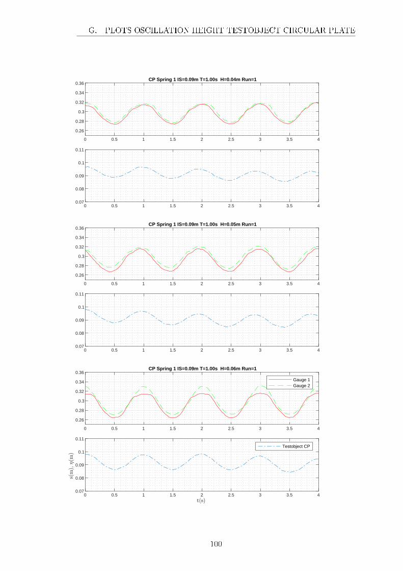
0 0.5 1 1.5 2 2.5 3 3.5 4
0.26
0.28
0.3
0.32
0.34
0.36 CP Spring 1 IS=0.09m T=1.00s H=0.04m Run=1
0 0.5 1 1.5 2 2.5 3 3.5 40.07
0.08
0.09
0.1
0.11
0 0.5 1 1.5 2 2.5 3 3.5 4
0.26
0.28
0.3
0.32
0.34
0.36 CP Spring 1 IS=0.09m T=1.00s H=0.05m Run=1
0 0.5 1 1.5 2 2.5 3 3.5 40.07
0.08
0.09
0.1
0.11
0 0.5 1 1.5 2 2.5 3 3.5 4
0.26
0.28
0.3
0.32
0.34
0.36 CP Spring 1 IS=0.09m T=1.00s H=0.06m Run=1
Gauge 1Gauge 2
0 0.5 1 1.5 2 2.5 3 3.5 40.07
0.08
0.09
0.1
0.11
Testobject CP
G. PLOTS OSCILLATION HEIGHT TESTOBJECT CIRCULAR PLATE
100
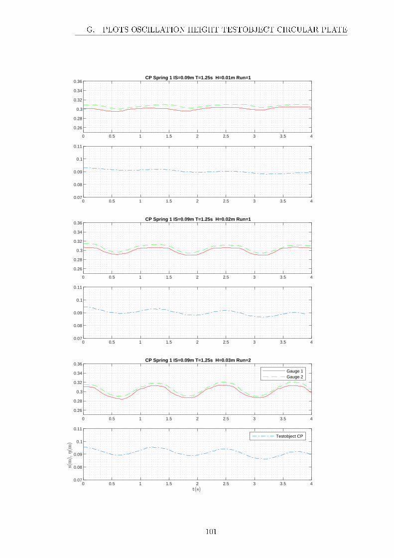
0 0.5 1 1.5 2 2.5 3 3.5 4
0.26
0.28
0.3
0.32
0.34
0.36 CP Spring 1 IS=0.09m T=1.25s H=0.01m Run=1
0 0.5 1 1.5 2 2.5 3 3.5 40.07
0.08
0.09
0.1
0.11
0 0.5 1 1.5 2 2.5 3 3.5 4
0.26
0.28
0.3
0.32
0.34
0.36 CP Spring 1 IS=0.09m T=1.25s H=0.02m Run=1
0 0.5 1 1.5 2 2.5 3 3.5 40.07
0.08
0.09
0.1
0.11
0 0.5 1 1.5 2 2.5 3 3.5 4
0.26
0.28
0.3
0.32
0.34
0.36 CP Spring 1 IS=0.09m T=1.25s H=0.03m Run=2
Gauge 1Gauge 2
0 0.5 1 1.5 2 2.5 3 3.5 40.07
0.08
0.09
0.1
0.11
Testobject CP
G. PLOTS OSCILLATION HEIGHT TESTOBJECT CIRCULAR PLATE
101

0 0.5 1 1.5 2 2.5 3 3.5 4
0.26
0.28
0.3
0.32
0.34
0.36 CP Spring 1 IS=0.09m T=1.25s H=0.04m Run=1
0 0.5 1 1.5 2 2.5 3 3.5 40.07
0.08
0.09
0.1
0.11
0 0.5 1 1.5 2 2.5 3 3.5 4
0.26
0.28
0.3
0.32
0.34
0.36 CP Spring 1 IS=0.09m T=1.25s H=0.05m Run=1
0 0.5 1 1.5 2 2.5 3 3.5 40.07
0.08
0.09
0.1
0.11
0 0.5 1 1.5 2 2.5 3 3.5 4
0.26
0.28
0.3
0.32
0.34
0.36 CP Spring 1 IS=0.09m T=1.25s H=0.06m Run=1
Gauge 1Gauge 2
0 0.5 1 1.5 2 2.5 3 3.5 40.07
0.08
0.09
0.1
0.11
Testobject CP
G. PLOTS OSCILLATION HEIGHT TESTOBJECT CIRCULAR PLATE
102
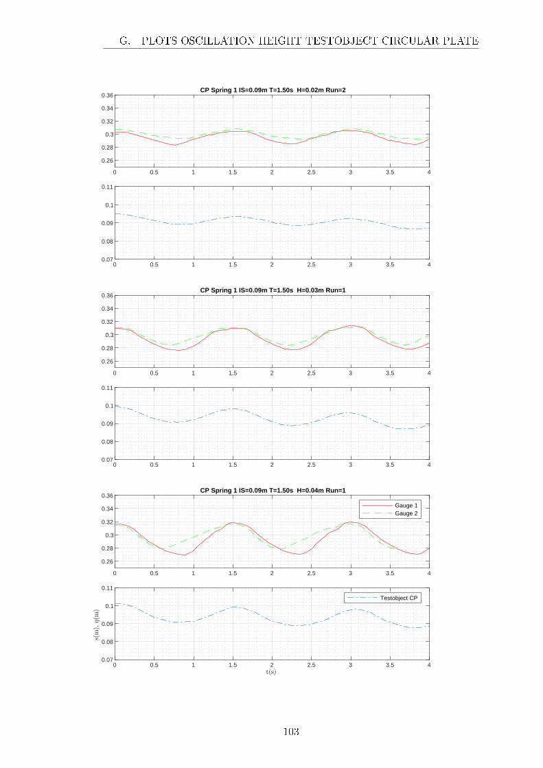
0 0.5 1 1.5 2 2.5 3 3.5 4
0.26
0.28
0.3
0.32
0.34
0.36 CP Spring 1 IS=0.09m T=1.50s H=0.02m Run=2
0 0.5 1 1.5 2 2.5 3 3.5 40.07
0.08
0.09
0.1
0.11
0 0.5 1 1.5 2 2.5 3 3.5 4
0.26
0.28
0.3
0.32
0.34
0.36 CP Spring 1 IS=0.09m T=1.50s H=0.03m Run=1
0 0.5 1 1.5 2 2.5 3 3.5 40.07
0.08
0.09
0.1
0.11
0 0.5 1 1.5 2 2.5 3 3.5 4
0.26
0.28
0.3
0.32
0.34
0.36 CP Spring 1 IS=0.09m T=1.50s H=0.04m Run=1
Gauge 1Gauge 2
0 0.5 1 1.5 2 2.5 3 3.5 40.07
0.08
0.09
0.1
0.11
Testobject CP
G. PLOTS OSCILLATION HEIGHT TESTOBJECT CIRCULAR PLATE
103

0 0.5 1 1.5 2 2.5 3 3.5 4
0.26
0.28
0.3
0.32
0.34
0.36 CP Spring 1 IS=0.09m T=1.50s H=0.05m Run=1
0 0.5 1 1.5 2 2.5 3 3.5 40.07
0.08
0.09
0.1
0.11
0 0.5 1 1.5 2 2.5 3 3.5 4
0.26
0.28
0.3
0.32
0.34
0.36 CP Spring 1 IS=0.09m T=1.50s H=0.06m Run=1
0 0.5 1 1.5 2 2.5 3 3.5 40.07
0.08
0.09
0.1
0.11
0 0.5 1 1.5 2 2.5 3 3.5 4
0.26
0.28
0.3
0.32
0.34
0.36 CP Spring 1 IS=0.09m T=1.75s H=0.02m Run=1
Gauge 1Gauge 2
0 0.5 1 1.5 2 2.5 3 3.5 40.07
0.08
0.09
0.1
0.11
Testobject CP
G. PLOTS OSCILLATION HEIGHT TESTOBJECT CIRCULAR PLATE
104

0 0.5 1 1.5 2 2.5 3 3.5 4
0.26
0.28
0.3
0.32
0.34
0.36 CP Spring 1 IS=0.09m T=1.75s H=0.03m Run=1
0 0.5 1 1.5 2 2.5 3 3.5 40.07
0.08
0.09
0.1
0.11
0 0.5 1 1.5 2 2.5 3 3.5 4
0.26
0.28
0.3
0.32
0.34
0.36 CP Spring 1 IS=0.09m T=1.75s H=0.04m Run=1
0 0.5 1 1.5 2 2.5 3 3.5 40.07
0.08
0.09
0.1
0.11
0 0.5 1 1.5 2 2.5 3 3.5 4
0.26
0.28
0.3
0.32
0.34
0.36 CP Spring 1 IS=0.09m T=1.75s H=0.05m Run=1
Gauge 1Gauge 2
0 0.5 1 1.5 2 2.5 3 3.5 40.07
0.08
0.09
0.1
0.11
Testobject CP
G. PLOTS OSCILLATION HEIGHT TESTOBJECT CIRCULAR PLATE
105

0 0.5 1 1.5 2 2.5 3 3.5 4
0.26
0.28
0.3
0.32
0.34
0.36 CP Spring 1 IS=0.09m T=1.75s H=0.06m Run=1
Gauge 1Gauge 2
0 0.5 1 1.5 2 2.5 3 3.5 40.07
0.08
0.09
0.1
0.11
Testobject CP
G. PLOTS OSCILLATION HEIGHT TESTOBJECT CIRCULAR PLATE
106

0 0.5 1 1.5 2 2.5 3 3.5 4
0.26
0.28
0.3
0.32
0.34 CP Spring 2 IS=0.27m T=0.70s H=0.01m Run=1
0 0.5 1 1.5 2 2.5 3 3.5 4
0.24
0.26
0.28
0.3
0 0.5 1 1.5 2 2.5 3 3.5 4
0.26
0.28
0.3
0.32
0.34 CP Spring 2 IS=0.27m T=0.70s H=0.02m Run=1
0 0.5 1 1.5 2 2.5 3 3.5 4
0.24
0.26
0.28
0.3
0 0.5 1 1.5 2 2.5 3 3.5 4
0.26
0.28
0.3
0.32
0.34 CP Spring 2 IS=0.27m T=0.70s H=0.03m Run=1
Gauge 1Gauge 2
0 0.5 1 1.5 2 2.5 3 3.5 4
0.24
0.26
0.28
0.3 Testobject CP
G. PLOTS OSCILLATION HEIGHT TESTOBJECT CIRCULAR PLATE
107

0 0.5 1 1.5 2 2.5 3 3.5 4
0.26
0.28
0.3
0.32
0.34 CP Spring 2 IS=0.27m T=0.70s H=0.04m Run=1
0 0.5 1 1.5 2 2.5 3 3.5 4
0.24
0.26
0.28
0.3
0 0.5 1 1.5 2 2.5 3 3.5 4
0.26
0.28
0.3
0.32
0.34 CP Spring 2 IS=0.27m T=0.70s H=0.05m Run=1
0 0.5 1 1.5 2 2.5 3 3.5 4
0.24
0.26
0.28
0.3
0 0.5 1 1.5 2 2.5 3 3.5 4
0.26
0.28
0.3
0.32
0.34 CP Spring 2 IS=0.27m T=0.70s H=0.06m Run=1
Gauge 1Gauge 2
0 0.5 1 1.5 2 2.5 3 3.5 4
0.24
0.26
0.28
0.3 Testobject CP
G. PLOTS OSCILLATION HEIGHT TESTOBJECT CIRCULAR PLATE
108
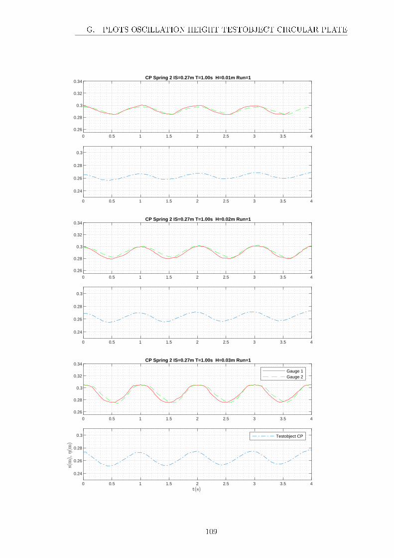
0 0.5 1 1.5 2 2.5 3 3.5 4
0.26
0.28
0.3
0.32
0.34 CP Spring 2 IS=0.27m T=1.00s H=0.01m Run=1
0 0.5 1 1.5 2 2.5 3 3.5 4
0.24
0.26
0.28
0.3
0 0.5 1 1.5 2 2.5 3 3.5 4
0.26
0.28
0.3
0.32
0.34 CP Spring 2 IS=0.27m T=1.00s H=0.02m Run=1
0 0.5 1 1.5 2 2.5 3 3.5 4
0.24
0.26
0.28
0.3
0 0.5 1 1.5 2 2.5 3 3.5 4
0.26
0.28
0.3
0.32
0.34 CP Spring 2 IS=0.27m T=1.00s H=0.03m Run=1
Gauge 1Gauge 2
0 0.5 1 1.5 2 2.5 3 3.5 4
0.24
0.26
0.28
0.3 Testobject CP
G. PLOTS OSCILLATION HEIGHT TESTOBJECT CIRCULAR PLATE
109

0 0.5 1 1.5 2 2.5 3 3.5 4
0.26
0.28
0.3
0.32
0.34 CP Spring 2 IS=0.27m T=1.00s H=0.04m Run=1
0 0.5 1 1.5 2 2.5 3 3.5 4
0.24
0.26
0.28
0.3
0 0.5 1 1.5 2 2.5 3 3.5 4
0.26
0.28
0.3
0.32
0.34 CP Spring 2 IS=0.27m T=1.00s H=0.05m Run=1
0 0.5 1 1.5 2 2.5 3 3.5 4
0.24
0.26
0.28
0.3
0 0.5 1 1.5 2 2.5 3 3.5 4
0.26
0.28
0.3
0.32
0.34 CP Spring 2 IS=0.27m T=1.00s H=0.06m Run=1
Gauge 1Gauge 2
0 0.5 1 1.5 2 2.5 3 3.5 4
0.24
0.26
0.28
0.3 Testobject CP
G. PLOTS OSCILLATION HEIGHT TESTOBJECT CIRCULAR PLATE
110

0 0.5 1 1.5 2 2.5 3 3.5 4
0.26
0.28
0.3
0.32
0.34 CP Spring 2 IS=0.27m T=1.25s H=0.01m Run=1
0 0.5 1 1.5 2 2.5 3 3.5 4
0.24
0.26
0.28
0.3
0 0.5 1 1.5 2 2.5 3 3.5 4
0.26
0.28
0.3
0.32
0.34 CP Spring 2 IS=0.27m T=1.25s H=0.02m Run=1
0 0.5 1 1.5 2 2.5 3 3.5 4
0.24
0.26
0.28
0.3
0 0.5 1 1.5 2 2.5 3 3.5 4
0.26
0.28
0.3
0.32
0.34 CP Spring 2 IS=0.27m T=1.25s H=0.03m Run=1
Gauge 1Gauge 2
0 0.5 1 1.5 2 2.5 3 3.5 4
0.24
0.26
0.28
0.3 Testobject CP
G. PLOTS OSCILLATION HEIGHT TESTOBJECT CIRCULAR PLATE
111
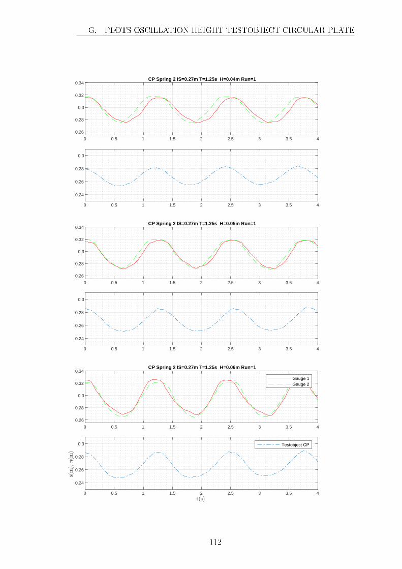
0 0.5 1 1.5 2 2.5 3 3.5 4
0.26
0.28
0.3
0.32
0.34 CP Spring 2 IS=0.27m T=1.25s H=0.04m Run=1
0 0.5 1 1.5 2 2.5 3 3.5 4
0.24
0.26
0.28
0.3
0 0.5 1 1.5 2 2.5 3 3.5 4
0.26
0.28
0.3
0.32
0.34 CP Spring 2 IS=0.27m T=1.25s H=0.05m Run=1
0 0.5 1 1.5 2 2.5 3 3.5 4
0.24
0.26
0.28
0.3
0 0.5 1 1.5 2 2.5 3 3.5 4
0.26
0.28
0.3
0.32
0.34 CP Spring 2 IS=0.27m T=1.25s H=0.06m Run=1
Gauge 1Gauge 2
0 0.5 1 1.5 2 2.5 3 3.5 4
0.24
0.26
0.28
0.3 Testobject CP
G. PLOTS OSCILLATION HEIGHT TESTOBJECT CIRCULAR PLATE
112
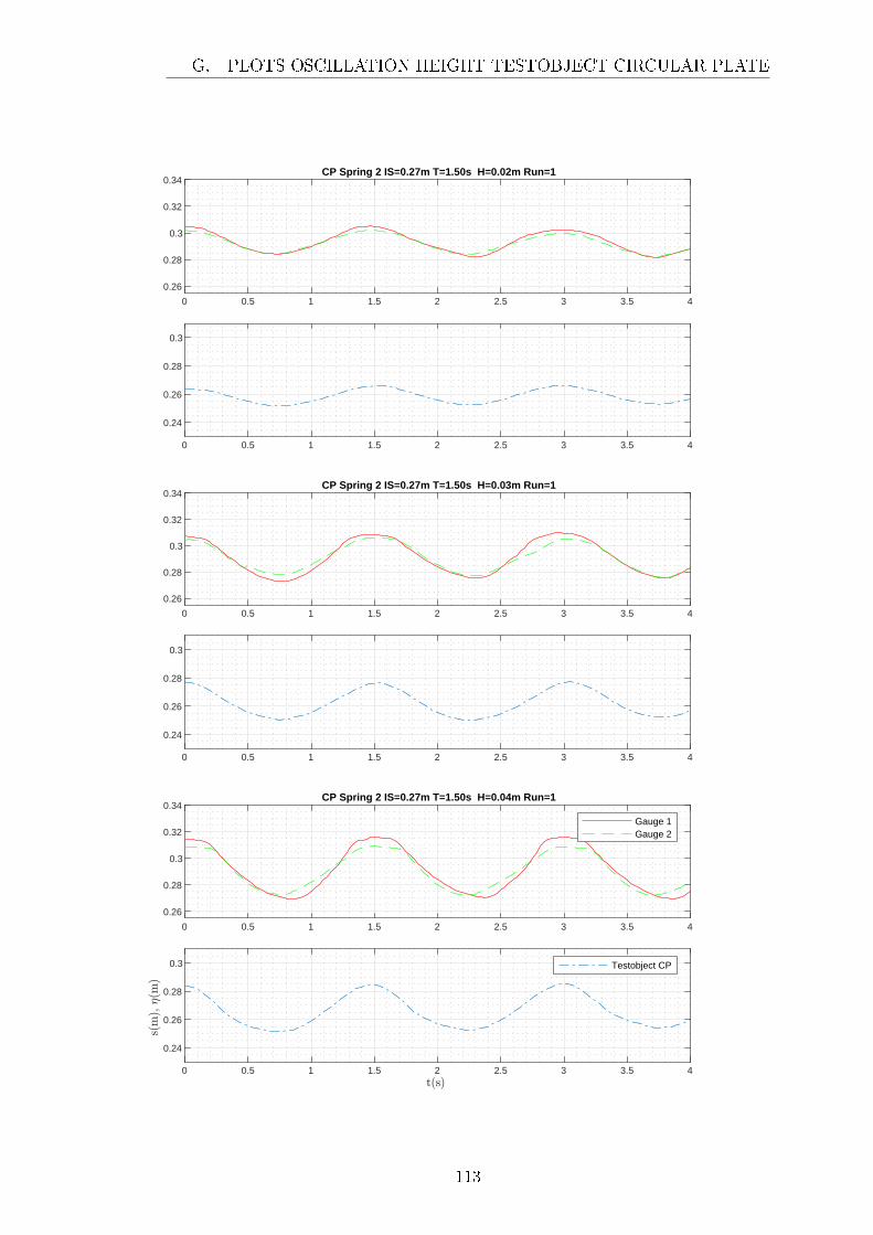
0 0.5 1 1.5 2 2.5 3 3.5 4
0.26
0.28
0.3
0.32
0.34 CP Spring 2 IS=0.27m T=1.50s H=0.02m Run=1
0 0.5 1 1.5 2 2.5 3 3.5 4
0.24
0.26
0.28
0.3
0 0.5 1 1.5 2 2.5 3 3.5 4
0.26
0.28
0.3
0.32
0.34 CP Spring 2 IS=0.27m T=1.50s H=0.03m Run=1
0 0.5 1 1.5 2 2.5 3 3.5 4
0.24
0.26
0.28
0.3
0 0.5 1 1.5 2 2.5 3 3.5 4
0.26
0.28
0.3
0.32
0.34 CP Spring 2 IS=0.27m T=1.50s H=0.04m Run=1
Gauge 1Gauge 2
0 0.5 1 1.5 2 2.5 3 3.5 4
0.24
0.26
0.28
0.3 Testobject CP
G. PLOTS OSCILLATION HEIGHT TESTOBJECT CIRCULAR PLATE
113

0 0.5 1 1.5 2 2.5 3 3.5 4
0.26
0.28
0.3
0.32
0.34 CP Spring 2 IS=0.27m T=1.50s H=0.05m Run=1
0 0.5 1 1.5 2 2.5 3 3.5 4
0.24
0.26
0.28
0.3
0 0.5 1 1.5 2 2.5 3 3.5 4
0.26
0.28
0.3
0.32
0.34 CP Spring 2 IS=0.27m T=1.50s H=0.06m Run=1
0 0.5 1 1.5 2 2.5 3 3.5 4
0.24
0.26
0.28
0.3
0 0.5 1 1.5 2 2.5 3 3.5 4
0.26
0.28
0.3
0.32
0.34 CP Spring 2 IS=0.27m T=1.75s H=0.02m Run=1
Gauge 1Gauge 2
0 0.5 1 1.5 2 2.5 3 3.5 4
0.24
0.26
0.28
0.3 Testobject CP
G. PLOTS OSCILLATION HEIGHT TESTOBJECT CIRCULAR PLATE
114

0 0.5 1 1.5 2 2.5 3 3.5 4
0.26
0.28
0.3
0.32
0.34 CP Spring 2 IS=0.27m T=1.75s H=0.03m Run=1
0 0.5 1 1.5 2 2.5 3 3.5 4
0.24
0.26
0.28
0.3
0 0.5 1 1.5 2 2.5 3 3.5 4
0.26
0.28
0.3
0.32
0.34 CP Spring 2 IS=0.27m T=1.75s H=0.04m Run=1
0 0.5 1 1.5 2 2.5 3 3.5 4
0.24
0.26
0.28
0.3
0 0.5 1 1.5 2 2.5 3 3.5 4
0.26
0.28
0.3
0.32
0.34 CP Spring 2 IS=0.27m T=1.75s H=0.05m Run=1
Gauge 1Gauge 2
0 0.5 1 1.5 2 2.5 3 3.5 4
0.24
0.26
0.28
0.3 Testobject CP
G. PLOTS OSCILLATION HEIGHT TESTOBJECT CIRCULAR PLATE
115

0 0.5 1 1.5 2 2.5 3 3.5 4
0.26
0.28
0.3
0.32
0.34
0.36 CP Spring 2 IS=0.027m T=1.75s H=0.06m Run=1
Gauge 1Gauge 2
0 0.5 1 1.5 2 2.5 3 3.5 4
0.24
0.26
0.28
0.3 Testobject CP
G. PLOTS OSCILLATION HEIGHT TESTOBJECT CIRCULAR PLATE
116
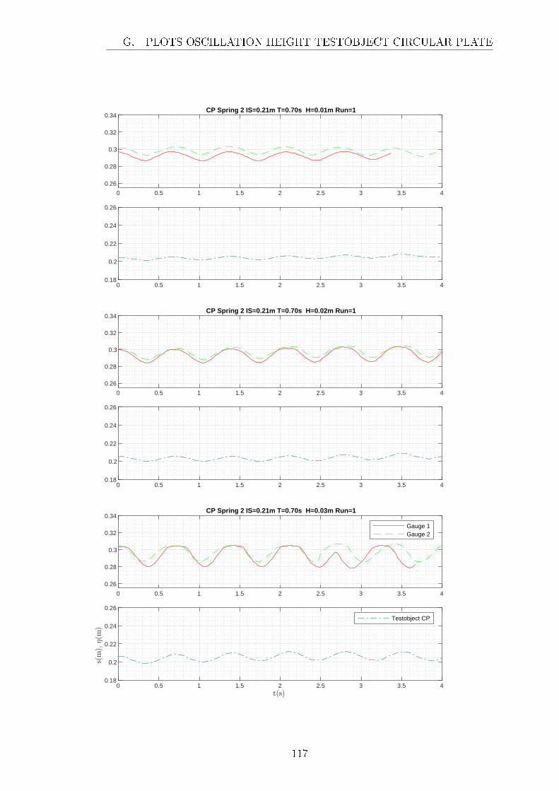
0 0.5 1 1.5 2 2.5 3 3.5 4
0.26
0.28
0.3
0.32
0.34 CP Spring 2 IS=0.21m T=0.70s H=0.01m Run=1
0 0.5 1 1.5 2 2.5 3 3.5 40.18
0.2
0.22
0.24
0.26
0 0.5 1 1.5 2 2.5 3 3.5 4
0.26
0.28
0.3
0.32
0.34 CP Spring 2 IS=0.21m T=0.70s H=0.02m Run=1
0 0.5 1 1.5 2 2.5 3 3.5 40.18
0.2
0.22
0.24
0.26
0 0.5 1 1.5 2 2.5 3 3.5 4
0.26
0.28
0.3
0.32
0.34 CP Spring 2 IS=0.21m T=0.70s H=0.03m Run=1
Gauge 1Gauge 2
0 0.5 1 1.5 2 2.5 3 3.5 40.18
0.2
0.22
0.24
0.26
Testobject CP
G. PLOTS OSCILLATION HEIGHT TESTOBJECT CIRCULAR PLATE
117

0 0.5 1 1.5 2 2.5 3 3.5 4
0.26
0.28
0.3
0.32
0.34 CP Spring 2 IS=0.21m T=0.70s H=0.04m Run=1
0 0.5 1 1.5 2 2.5 3 3.5 40.18
0.2
0.22
0.24
0.26
0 0.5 1 1.5 2 2.5 3 3.5 4
0.26
0.28
0.3
0.32
0.34 CP Spring 2 IS=0.21m T=0.70s H=0.05m Run=1
0 0.5 1 1.5 2 2.5 3 3.5 40.18
0.2
0.22
0.24
0.26
0 0.5 1 1.5 2 2.5 3 3.5 4
0.26
0.28
0.3
0.32
0.34 CP Spring 2 IS=0.21m T=0.70s H=0.06m Run=1
Gauge 1Gauge 2
0 0.5 1 1.5 2 2.5 3 3.5 40.18
0.2
0.22
0.24
0.26
Testobject CP
G. PLOTS OSCILLATION HEIGHT TESTOBJECT CIRCULAR PLATE
118
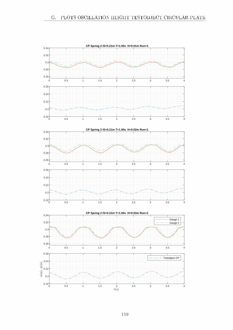
0 0.5 1 1.5 2 2.5 3 3.5 4
0.26
0.28
0.3
0.32
0.34 CP Spring 2 IS=0.21m T=1.00s H=0.01m Run=1
0 0.5 1 1.5 2 2.5 3 3.5 40.18
0.2
0.22
0.24
0.26
0 0.5 1 1.5 2 2.5 3 3.5 4
0.26
0.28
0.3
0.32
0.34 CP Spring 2 IS=0.21m T=1.00s H=0.02m Run=1
0 0.5 1 1.5 2 2.5 3 3.5 40.18
0.2
0.22
0.24
0.26
0 0.5 1 1.5 2 2.5 3 3.5 4
0.26
0.28
0.3
0.32
0.34 CP Spring 2 IS=0.21m T=1.00s H=0.03m Run=1
Gauge 1Gauge 2
0 0.5 1 1.5 2 2.5 3 3.5 40.18
0.2
0.22
0.24
0.26
Testobject CP
G. PLOTS OSCILLATION HEIGHT TESTOBJECT CIRCULAR PLATE
119

0 0.5 1 1.5 2 2.5 3 3.5 4
0.26
0.28
0.3
0.32
0.34 CP Spring 2 IS=0.21m T=1.00s H=0.04m Run=1
0 0.5 1 1.5 2 2.5 3 3.5 40.18
0.2
0.22
0.24
0.26
0 0.5 1 1.5 2 2.5 3 3.5 4
0.26
0.28
0.3
0.32
0.34 CP Spring 2 IS=0.21m T=1.00s H=0.05m Run=1
0 0.5 1 1.5 2 2.5 3 3.5 40.18
0.2
0.22
0.24
0.26
0 0.5 1 1.5 2 2.5 3 3.5 4
0.26
0.28
0.3
0.32
0.34 CP Spring 2 IS=0.21m T=1.00s H=0.06m Run=1
Gauge 1Gauge 2
0 0.5 1 1.5 2 2.5 3 3.5 40.18
0.2
0.22
0.24
0.26
Testobject CP
G. PLOTS OSCILLATION HEIGHT TESTOBJECT CIRCULAR PLATE
120
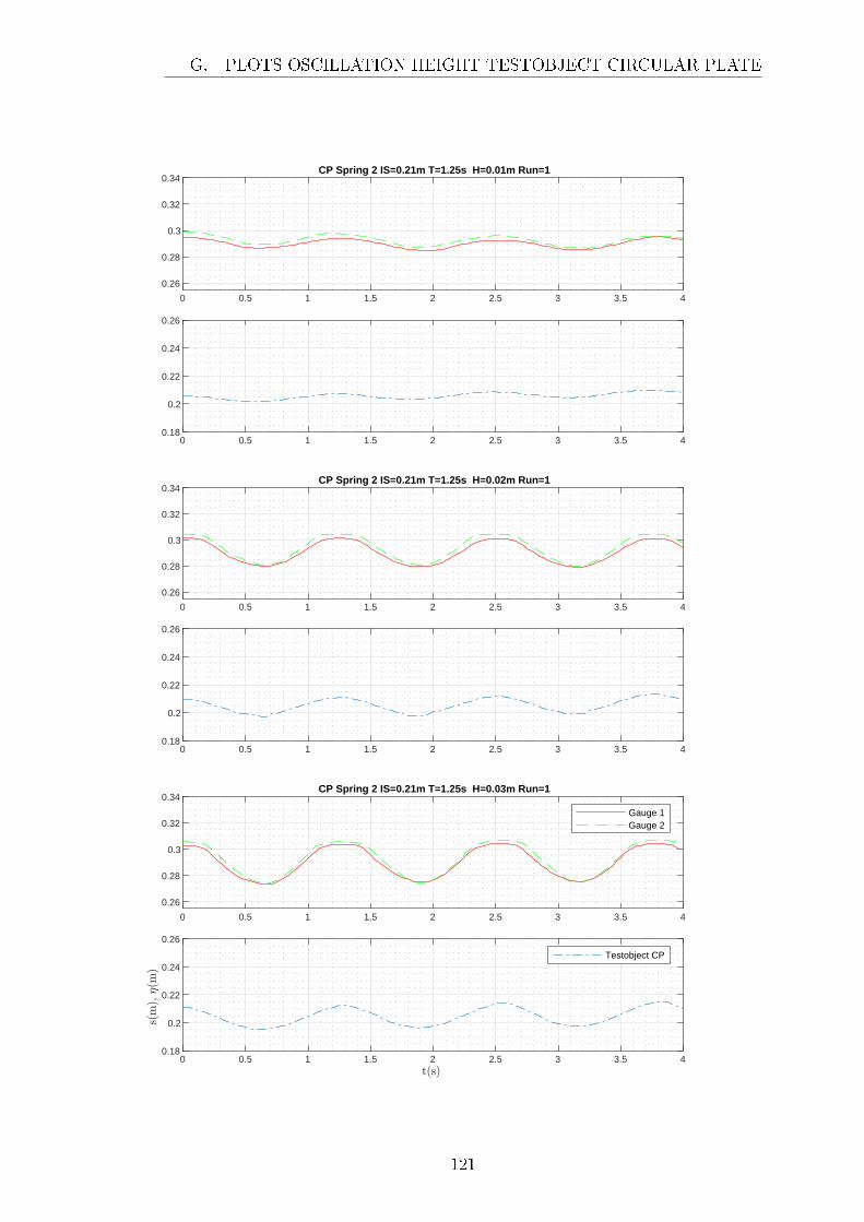
0 0.5 1 1.5 2 2.5 3 3.5 4
0.26
0.28
0.3
0.32
0.34 CP Spring 2 IS=0.21m T=1.25s H=0.01m Run=1
0 0.5 1 1.5 2 2.5 3 3.5 40.18
0.2
0.22
0.24
0.26
0 0.5 1 1.5 2 2.5 3 3.5 4
0.26
0.28
0.3
0.32
0.34 CP Spring 2 IS=0.21m T=1.25s H=0.02m Run=1
0 0.5 1 1.5 2 2.5 3 3.5 40.18
0.2
0.22
0.24
0.26
0 0.5 1 1.5 2 2.5 3 3.5 4
0.26
0.28
0.3
0.32
0.34 CP Spring 2 IS=0.21m T=1.25s H=0.03m Run=1
Gauge 1Gauge 2
0 0.5 1 1.5 2 2.5 3 3.5 40.18
0.2
0.22
0.24
0.26
Testobject CP
G. PLOTS OSCILLATION HEIGHT TESTOBJECT CIRCULAR PLATE
121

0 0.5 1 1.5 2 2.5 3 3.5 4
0.26
0.28
0.3
0.32
0.34
0.36 CP Spring 2 IS=0.21m T=1.25s H=0.04m Run=1
0 0.5 1 1.5 2 2.5 3 3.5 40.18
0.2
0.22
0.24
0.26
0 0.5 1 1.5 2 2.5 3 3.5 4
0.26
0.28
0.3
0.32
0.34
0.36 CP Spring 2 IS=0.21m T=1.25s H=0.05m Run=1
0 0.5 1 1.5 2 2.5 3 3.5 40.18
0.2
0.22
0.24
0.26
0 0.5 1 1.5 2 2.5 3 3.5 4
0.26
0.28
0.3
0.32
0.34
0.36 CP Spring 2 IS=0.21m T=1.25s H=0.06m Run=1
Gauge 1Gauge 2
0 0.5 1 1.5 2 2.5 3 3.5 40.18
0.2
0.22
0.24
0.26
Testobject CP
G. PLOTS OSCILLATION HEIGHT TESTOBJECT CIRCULAR PLATE
122

0 0.5 1 1.5 2 2.5 3 3.5 4
0.26
0.28
0.3
0.32
0.34 CP Spring 2 IS=0.21m T=1.50s H=0.02m Run=1
0 0.5 1 1.5 2 2.5 3 3.5 40.18
0.2
0.22
0.24
0.26
0 0.5 1 1.5 2 2.5 3 3.5 4
0.26
0.28
0.3
0.32
0.34 CP Spring 2 IS=0.21m T=1.50s H=0.03m Run=1
0 0.5 1 1.5 2 2.5 3 3.5 40.18
0.2
0.22
0.24
0.26
0 0.5 1 1.5 2 2.5 3 3.5 4
0.26
0.28
0.3
0.32
0.34 CP Spring 2 IS=0.21m T=1.50s H=0.04m Run=1
Gauge 1Gauge 2
0 0.5 1 1.5 2 2.5 3 3.5 40.18
0.2
0.22
0.24
0.26
Testobject CP
G. PLOTS OSCILLATION HEIGHT TESTOBJECT CIRCULAR PLATE
123
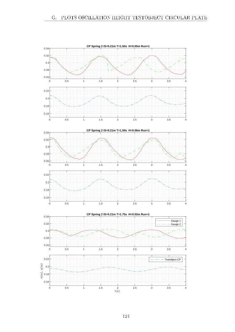
0 0.5 1 1.5 2 2.5 3 3.5 4
0.26
0.28
0.3
0.32
0.34 CP Spring 2 IS=0.21m T=1.50s H=0.05m Run=1
0 0.5 1 1.5 2 2.5 3 3.5 4
0.16
0.18
0.2
0.22
0 0.5 1 1.5 2 2.5 3 3.5 4
0.26
0.28
0.3
0.32
0.34 CP Spring 2 IS=0.21m T=1.50s H=0.06m Run=1
0 0.5 1 1.5 2 2.5 3 3.5 4
0.16
0.18
0.2
0.22
0 0.5 1 1.5 2 2.5 3 3.5 4
0.26
0.28
0.3
0.32
0.34 CP Spring 2 IS=0.21m T=1.75s H=0.02m Run=1
Gauge 1Gauge 2
0 0.5 1 1.5 2 2.5 3 3.5 4
0.16
0.18
0.2
0.22 Testobject CP
G. PLOTS OSCILLATION HEIGHT TESTOBJECT CIRCULAR PLATE
124

0 0.5 1 1.5 2 2.5 3 3.5 4
0.26
0.28
0.3
0.32
0.34 CP Spring 2 IS=0.21m T=1.75s H=0.03m Run=1
0 0.5 1 1.5 2 2.5 3 3.5 4
0.16
0.18
0.2
0.22
0 0.5 1 1.5 2 2.5 3 3.5 4
0.26
0.28
0.3
0.32
0.34 CP Spring 2 IS=0.21m T=1.75s H=0.04m Run=1
0 0.5 1 1.5 2 2.5 3 3.5 4
0.16
0.18
0.2
0.22
0 0.5 1 1.5 2 2.5 3 3.5 4
0.26
0.28
0.3
0.32
0.34 CP Spring 2 IS=0.21m T=1.75s H=0.05m Run=1
Gauge 1Gauge 2
0 0.5 1 1.5 2 2.5 3 3.5 4
0.16
0.18
0.2
0.22 Testobject CP
G. PLOTS OSCILLATION HEIGHT TESTOBJECT CIRCULAR PLATE
125
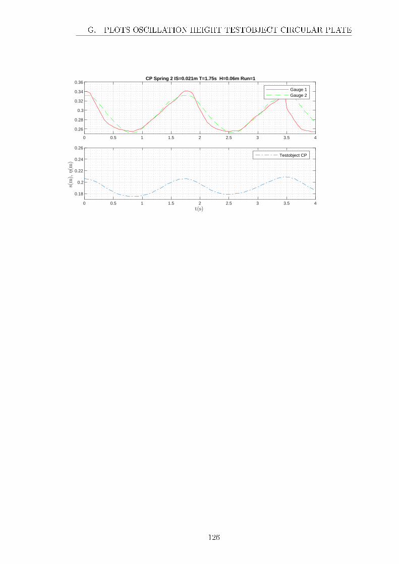
0 0.5 1 1.5 2 2.5 3 3.5 4
0.26
0.28
0.3
0.32
0.34
0.36 CP Spring 2 IS=0.021m T=1.75s H=0.06m Run=1
Gauge 1Gauge 2
0 0.5 1 1.5 2 2.5 3 3.5 4
0.18
0.2
0.22
0.24
0.26
Testobject CP
G. PLOTS OSCILLATION HEIGHT TESTOBJECT CIRCULAR PLATE
126

0 0.5 1 1.5 2 2.5 3 3.5 4
0.26
0.28
0.3
0.32
0.34 CP Spring 2 IS=0.15m T=0.70s H=0.01m Run=1
0 0.5 1 1.5 2 2.5 3 3.5 40.12
0.14
0.16
0.18
0 0.5 1 1.5 2 2.5 3 3.5 4
0.26
0.28
0.3
0.32
0.34 CP Spring 2 IS=0.15m T=0.70s H=0.02m Run=1
0 0.5 1 1.5 2 2.5 3 3.5 40.12
0.14
0.16
0.18
0 0.5 1 1.5 2 2.5 3 3.5 4
0.26
0.28
0.3
0.32
0.34 CP Spring 2 IS=0.15m T=0.70s H=0.03m Run=1
Gauge 1Gauge 2
0 0.5 1 1.5 2 2.5 3 3.5 40.12
0.14
0.16
0.18
Testobject CP
G. PLOTS OSCILLATION HEIGHT TESTOBJECT CIRCULAR PLATE
127

0 0.5 1 1.5 2 2.5 3 3.5 4
0.26
0.28
0.3
0.32
0.34
0.36 CP Spring 2 IS=0.15m T=0.70s H=0.04m Run=1
0 0.5 1 1.5 2 2.5 3 3.5 40.12
0.14
0.16
0.18
0 0.5 1 1.5 2 2.5 3 3.5 4
0.26
0.28
0.3
0.32
0.34
0.36 CP Spring 2 IS=0.15m T=0.70s H=0.05m Run=1
0 0.5 1 1.5 2 2.5 3 3.5 40.12
0.14
0.16
0.18
0 0.5 1 1.5 2 2.5 3 3.5 4
0.26
0.28
0.3
0.32
0.34
0.36 CP Spring 2 IS=0.15m T=0.70s H=0.06m Run=1
Gauge 1Gauge 2
0 0.5 1 1.5 2 2.5 3 3.5 40.12
0.14
0.16
0.18
Testobject CP
G. PLOTS OSCILLATION HEIGHT TESTOBJECT CIRCULAR PLATE
128

0 0.5 1 1.5 2 2.5 3 3.5 4
0.26
0.28
0.3
0.32
0.34 CP Spring 2 IS=0.15m T=1.00s H=0.01m Run=1
0 0.5 1 1.5 2 2.5 3 3.5 40.142
0.144
0.146
0.148
0.15
0 0.5 1 1.5 2 2.5 3 3.5 4
0.26
0.28
0.3
0.32
0.34 CP Spring 2 IS=0.15m T=1.00s H=0.02m Run=1
0 0.5 1 1.5 2 2.5 3 3.5 40.14
0.145
0.15
0 0.5 1 1.5 2 2.5 3 3.5 4
0.26
0.28
0.3
0.32
0.34 CP Spring 2 IS=0.15m T=1.00s H=0.03m Run=1
Gauge 1Gauge 2
0 0.5 1 1.5 2 2.5 3 3.5 4
0.14
0.145
0.15
Testobject CP
G. PLOTS OSCILLATION HEIGHT TESTOBJECT CIRCULAR PLATE
129

0 0.5 1 1.5 2 2.5 3 3.5 4
0.26
0.28
0.3
0.32
0.34 CP Spring 2 IS=0.15m T=1.00s H=0.04m Run=1
0 0.5 1 1.5 2 2.5 3 3.5 4
0.14
0.145
0.15
0.155
0 0.5 1 1.5 2 2.5 3 3.5 4
0.26
0.28
0.3
0.32
0.34 CP Spring 2 IS=0.15m T=1.00s H=0.05m Run=1
0 0.5 1 1.5 2 2.5 3 3.5 4
0.14
0.145
0.15
0.155
0 0.5 1 1.5 2 2.5 3 3.5 4
0.26
0.28
0.3
0.32
0.34 CP Spring 2 IS=0.15m T=1.00s H=0.06m Run=1
Gauge 1Gauge 2
0 0.5 1 1.5 2 2.5 3 3.5 4
0.135
0.14
0.145
0.15
0.155 Testobject CP
G. PLOTS OSCILLATION HEIGHT TESTOBJECT CIRCULAR PLATE
130

0 0.5 1 1.5 2 2.5 3 3.5 4
0.26
0.28
0.3
0.32
0.34 CP Spring 2 IS=0.15m T=1.25s H=0.01m Run=1
0 0.5 1 1.5 2 2.5 3 3.5 40.12
0.14
0.16
0.18
0 0.5 1 1.5 2 2.5 3 3.5 4
0.26
0.28
0.3
0.32
0.34 CP Spring 2 IS=0.15m T=1.25s H=0.02m Run=1
0 0.5 1 1.5 2 2.5 3 3.5 40.12
0.14
0.16
0.18
0 0.5 1 1.5 2 2.5 3 3.5 4
0.26
0.28
0.3
0.32
0.34 CP Spring 2 IS=0.15m T=1.25s H=0.03m Run=1
Gauge 1Gauge 2
0 0.5 1 1.5 2 2.5 3 3.5 40.12
0.14
0.16
0.18
Testobject CP
G. PLOTS OSCILLATION HEIGHT TESTOBJECT CIRCULAR PLATE
131
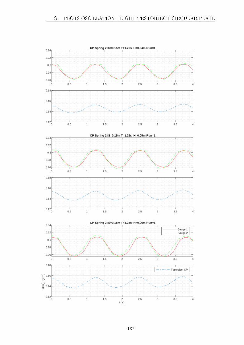
0 0.5 1 1.5 2 2.5 3 3.5 4
0.26
0.28
0.3
0.32
0.34 CP Spring 2 IS=0.15m T=1.25s H=0.04m Run=1
0 0.5 1 1.5 2 2.5 3 3.5 40.12
0.14
0.16
0.18
0 0.5 1 1.5 2 2.5 3 3.5 4
0.26
0.28
0.3
0.32
0.34 CP Spring 2 IS=0.15m T=1.25s H=0.05m Run=1
0 0.5 1 1.5 2 2.5 3 3.5 40.12
0.14
0.16
0.18
0 0.5 1 1.5 2 2.5 3 3.5 4
0.26
0.28
0.3
0.32
0.34 CP Spring 2 IS=0.15m T=1.25s H=0.06m Run=1
Gauge 1Gauge 2
0 0.5 1 1.5 2 2.5 3 3.5 40.12
0.14
0.16
0.18
Testobject CP
G. PLOTS OSCILLATION HEIGHT TESTOBJECT CIRCULAR PLATE
132

0 0.5 1 1.5 2 2.5 3 3.5 4
0.26
0.28
0.3
0.32
0.34 CP Spring 2 IS=0.15m T=1.50s H=0.02m Run=1
0 0.5 1 1.5 2 2.5 3 3.5 40.12
0.14
0.16
0.18
0 0.5 1 1.5 2 2.5 3 3.5 4
0.26
0.28
0.3
0.32
0.34 CP Spring 2 IS=0.15m T=1.50s H=0.03m Run=1
0 0.5 1 1.5 2 2.5 3 3.5 40.12
0.14
0.16
0.18
0 0.5 1 1.5 2 2.5 3 3.5 4
0.26
0.28
0.3
0.32
0.34 CP Spring 2 IS=0.15m T=1.50s H=0.04m Run=1
Gauge 1Gauge 2
0 0.5 1 1.5 2 2.5 3 3.5 40.12
0.14
0.16
0.18
Testobject CP
G. PLOTS OSCILLATION HEIGHT TESTOBJECT CIRCULAR PLATE
133

0 0.5 1 1.5 2 2.5 3 3.5 4
0.26
0.28
0.3
0.32
0.34 CP Spring 2 IS=0.15m T=1.50s H=0.05m Run=1
0 0.5 1 1.5 2 2.5 3 3.5 40.12
0.14
0.16
0.18
0 0.5 1 1.5 2 2.5 3 3.5 4
0.26
0.28
0.3
0.32
0.34 CP Spring 2 IS=0.15m T=1.50s H=0.06m Run=1
0 0.5 1 1.5 2 2.5 3 3.5 40.12
0.14
0.16
0.18
0 0.5 1 1.5 2 2.5 3 3.5 4
0.26
0.28
0.3
0.32
0.34 CP Spring 2 IS=0.15m T=1.75s H=0.02m Run=1
Gauge 1Gauge 2
0 0.5 1 1.5 2 2.5 3 3.5 40.12
0.14
0.16
0.18
Testobject CP
G. PLOTS OSCILLATION HEIGHT TESTOBJECT CIRCULAR PLATE
134

0 0.5 1 1.5 2 2.5 3 3.5 4
0.26
0.28
0.3
0.32
0.34 CP Spring 2 IS=0.15m T=1.75s H=0.03m Run=1
0 0.5 1 1.5 2 2.5 3 3.5 40.12
0.14
0.16
0.18
0 0.5 1 1.5 2 2.5 3 3.5 4
0.26
0.28
0.3
0.32
0.34 CP Spring 2 IS=0.15m T=1.75s H=0.04m Run=1
0 0.5 1 1.5 2 2.5 3 3.5 40.12
0.14
0.16
0.18
0 0.5 1 1.5 2 2.5 3 3.5 4
0.26
0.28
0.3
0.32
0.34 CP Spring 2 IS=0.15m T=1.75s H=0.05m Run=1
Gauge 1Gauge 2
0 0.5 1 1.5 2 2.5 3 3.5 40.12
0.14
0.16
0.18
Testobject CP
G. PLOTS OSCILLATION HEIGHT TESTOBJECT CIRCULAR PLATE
135
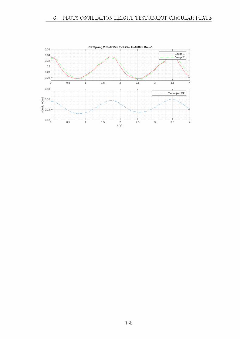
0 0.5 1 1.5 2 2.5 3 3.5 4
0.26
0.28
0.3
0.32
0.34
0.36 CP Spring 2 IS=0.15m T=1.75s H=0.06m Run=1
Gauge 1Gauge 2
0 0.5 1 1.5 2 2.5 3 3.5 40.12
0.14
0.16
0.18
Testobject CP
G. PLOTS OSCILLATION HEIGHT TESTOBJECT CIRCULAR PLATE
136

0 0.5 1 1.5 2 2.5 3 3.5 4
0.26
0.28
0.3
0.32
0.34 CP Spring 2 IS=0.09m T=0.70s H=0.01m Run=1
0 0.5 1 1.5 2 2.5 3 3.5 4
0.06
0.08
0.1
0.12
0 0.5 1 1.5 2 2.5 3 3.5 4
0.26
0.28
0.3
0.32
0.34 CP Spring 2 IS=0.09m T=0.70s H=0.02m Run=1
0 0.5 1 1.5 2 2.5 3 3.5 4
0.06
0.08
0.1
0.12
0 0.5 1 1.5 2 2.5 3 3.5 4
0.26
0.28
0.3
0.32
0.34 CP Spring 2 IS=0.09m T=0.70s H=0.03m Run=1
Gauge 1Gauge 2
0 0.5 1 1.5 2 2.5 3 3.5 4
0.06
0.08
0.1
0.12 Testobject CP
G. PLOTS OSCILLATION HEIGHT TESTOBJECT CIRCULAR PLATE
137
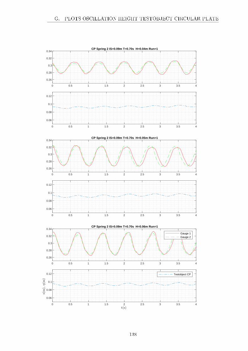
0 0.5 1 1.5 2 2.5 3 3.5 4
0.26
0.28
0.3
0.32
0.34 CP Spring 2 IS=0.09m T=0.70s H=0.04m Run=1
0 0.5 1 1.5 2 2.5 3 3.5 4
0.06
0.08
0.1
0.12
0 0.5 1 1.5 2 2.5 3 3.5 4
0.26
0.28
0.3
0.32
0.34 CP Spring 2 IS=0.09m T=0.70s H=0.05m Run=1
0 0.5 1 1.5 2 2.5 3 3.5 4
0.06
0.08
0.1
0.12
0 0.5 1 1.5 2 2.5 3 3.5 4
0.26
0.28
0.3
0.32
0.34 CP Spring 2 IS=0.09m T=0.70s H=0.06m Run=1
Gauge 1Gauge 2
0 0.5 1 1.5 2 2.5 3 3.5 4
0.06
0.08
0.1
0.12 Testobject CP
G. PLOTS OSCILLATION HEIGHT TESTOBJECT CIRCULAR PLATE
138
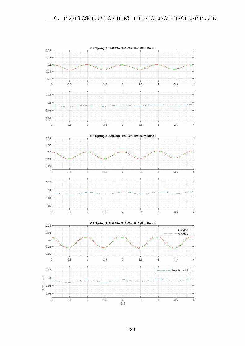
0 0.5 1 1.5 2 2.5 3 3.5 4
0.26
0.28
0.3
0.32
0.34 CP Spring 2 IS=0.09m T=1.00s H=0.01m Run=1
0 0.5 1 1.5 2 2.5 3 3.5 4
0.06
0.08
0.1
0.12
0 0.5 1 1.5 2 2.5 3 3.5 4
0.26
0.28
0.3
0.32
0.34 CP Spring 2 IS=0.09m T=1.00s H=0.02m Run=1
0 0.5 1 1.5 2 2.5 3 3.5 4
0.06
0.08
0.1
0.12
0 0.5 1 1.5 2 2.5 3 3.5 4
0.26
0.28
0.3
0.32
0.34 CP Spring 2 IS=0.09m T=1.00s H=0.03m Run=1
Gauge 1Gauge 2
0 0.5 1 1.5 2 2.5 3 3.5 4
0.06
0.08
0.1
0.12 Testobject CP
G. PLOTS OSCILLATION HEIGHT TESTOBJECT CIRCULAR PLATE
139
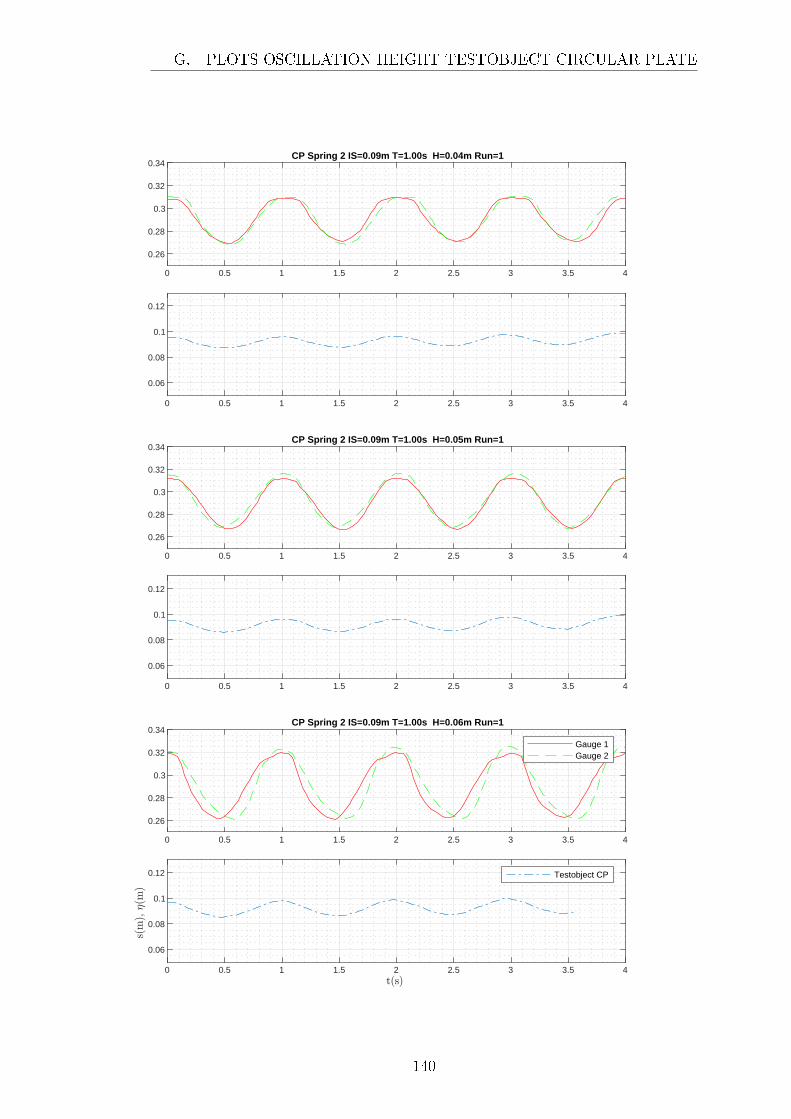
0 0.5 1 1.5 2 2.5 3 3.5 4
0.26
0.28
0.3
0.32
0.34 CP Spring 2 IS=0.09m T=1.00s H=0.04m Run=1
0 0.5 1 1.5 2 2.5 3 3.5 4
0.06
0.08
0.1
0.12
0 0.5 1 1.5 2 2.5 3 3.5 4
0.26
0.28
0.3
0.32
0.34 CP Spring 2 IS=0.09m T=1.00s H=0.05m Run=1
0 0.5 1 1.5 2 2.5 3 3.5 4
0.06
0.08
0.1
0.12
0 0.5 1 1.5 2 2.5 3 3.5 4
0.26
0.28
0.3
0.32
0.34 CP Spring 2 IS=0.09m T=1.00s H=0.06m Run=1
Gauge 1Gauge 2
0 0.5 1 1.5 2 2.5 3 3.5 4
0.06
0.08
0.1
0.12 Testobject CP
G. PLOTS OSCILLATION HEIGHT TESTOBJECT CIRCULAR PLATE
140

0 0.5 1 1.5 2 2.5 3 3.5 4
0.26
0.28
0.3
0.32
0.34 CP Spring 2 IS=0.09m T=1.25s H=0.01m Run=1
0 0.5 1 1.5 2 2.5 3 3.5 4
0.06
0.08
0.1
0.12
0 0.5 1 1.5 2 2.5 3 3.5 4
0.26
0.28
0.3
0.32
0.34 CP Spring 2 IS=0.09m T=1.25s H=0.02m Run=1
0 0.5 1 1.5 2 2.5 3 3.5 4
0.06
0.08
0.1
0.12
0 0.5 1 1.5 2 2.5 3 3.5 4
0.26
0.28
0.3
0.32
0.34 CP Spring 2 IS=0.09m T=1.25s H=0.03m Run=1
Gauge 1Gauge 2
0 0.5 1 1.5 2 2.5 3 3.5 4
0.06
0.08
0.1
0.12 Testobject CP
G. PLOTS OSCILLATION HEIGHT TESTOBJECT CIRCULAR PLATE
141
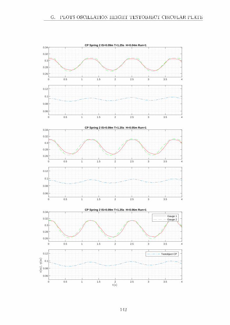
0 0.5 1 1.5 2 2.5 3 3.5 4
0.26
0.28
0.3
0.32
0.34 CP Spring 2 IS=0.09m T=1.25s H=0.04m Run=1
0 0.5 1 1.5 2 2.5 3 3.5 4
0.06
0.08
0.1
0.12
0 0.5 1 1.5 2 2.5 3 3.5 4
0.26
0.28
0.3
0.32
0.34 CP Spring 2 IS=0.09m T=1.25s H=0.05m Run=1
0 0.5 1 1.5 2 2.5 3 3.5 4
0.06
0.08
0.1
0.12
0 0.5 1 1.5 2 2.5 3 3.5 4
0.26
0.28
0.3
0.32
0.34 CP Spring 2 IS=0.09m T=1.25s H=0.06m Run=1
Gauge 1Gauge 2
0 0.5 1 1.5 2 2.5 3 3.5 4
0.06
0.08
0.1
0.12 Testobject CP
G. PLOTS OSCILLATION HEIGHT TESTOBJECT CIRCULAR PLATE
142
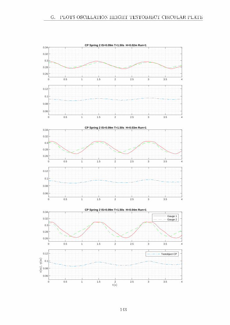
0 0.5 1 1.5 2 2.5 3 3.5 4
0.26
0.28
0.3
0.32
0.34 CP Spring 2 IS=0.09m T=1.50s H=0.02m Run=1
0 0.5 1 1.5 2 2.5 3 3.5 4
0.06
0.08
0.1
0.12
0 0.5 1 1.5 2 2.5 3 3.5 4
0.26
0.28
0.3
0.32
0.34 CP Spring 2 IS=0.09m T=1.50s H=0.03m Run=1
0 0.5 1 1.5 2 2.5 3 3.5 4
0.06
0.08
0.1
0.12
0 0.5 1 1.5 2 2.5 3 3.5 4
0.26
0.28
0.3
0.32
0.34 CP Spring 2 IS=0.09m T=1.50s H=0.04m Run=1
Gauge 1Gauge 2
0 0.5 1 1.5 2 2.5 3 3.5 4
0.06
0.08
0.1
0.12 Testobject CP
G. PLOTS OSCILLATION HEIGHT TESTOBJECT CIRCULAR PLATE
143
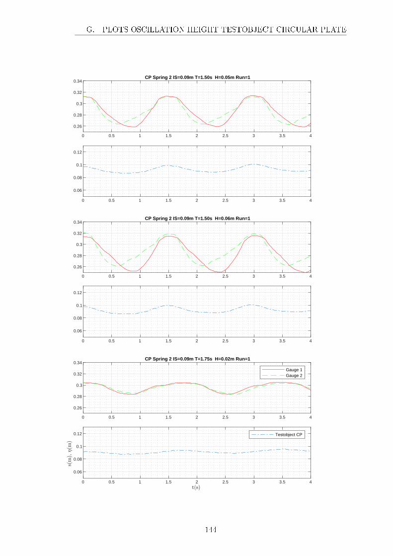
0 0.5 1 1.5 2 2.5 3 3.5 4
0.26
0.28
0.3
0.32
0.34 CP Spring 2 IS=0.09m T=1.50s H=0.05m Run=1
0 0.5 1 1.5 2 2.5 3 3.5 4
0.06
0.08
0.1
0.12
0 0.5 1 1.5 2 2.5 3 3.5 4
0.26
0.28
0.3
0.32
0.34 CP Spring 2 IS=0.09m T=1.50s H=0.06m Run=1
0 0.5 1 1.5 2 2.5 3 3.5 4
0.06
0.08
0.1
0.12
0 0.5 1 1.5 2 2.5 3 3.5 4
0.26
0.28
0.3
0.32
0.34 CP Spring 2 IS=0.09m T=1.75s H=0.02m Run=1
Gauge 1Gauge 2
0 0.5 1 1.5 2 2.5 3 3.5 4
0.06
0.08
0.1
0.12 Testobject CP
G. PLOTS OSCILLATION HEIGHT TESTOBJECT CIRCULAR PLATE
144

0 0.5 1 1.5 2 2.5 3 3.5 4
0.26
0.28
0.3
0.32
0.34 CP Spring 2 IS=0.09m T=1.75s H=0.03m Run=1
0 0.5 1 1.5 2 2.5 3 3.5 4
0.06
0.08
0.1
0.12
0 0.5 1 1.5 2 2.5 3 3.5 4
0.26
0.28
0.3
0.32
0.34 CP Spring 2 IS=0.09m T=1.75s H=0.04m Run=1
0 0.5 1 1.5 2 2.5 3 3.5 4
0.06
0.08
0.1
0.12
0 0.5 1 1.5 2 2.5 3 3.5 4
0.26
0.28
0.3
0.32
0.34 CP Spring 2 IS=0.09m T=1.75s H=0.05m Run=1
Gauge 1Gauge 2
0 0.5 1 1.5 2 2.5 3 3.5 4
0.06
0.08
0.1
0.12 Testobject CP
G. PLOTS OSCILLATION HEIGHT TESTOBJECT CIRCULAR PLATE
145

0 0.5 1 1.5 2 2.5 3 3.5 4
0.26
0.28
0.3
0.32
0.34
0.36 CP Spring 2 IS=0.09m T=1.75s H=0.06m Run=1
Gauge 1Gauge 2
0 0.5 1 1.5 2 2.5 3 3.5 4
0.06
0.08
0.1
0.12 Testobject CP
G. PLOTS OSCILLATION HEIGHT TESTOBJECT CIRCULAR PLATE
146
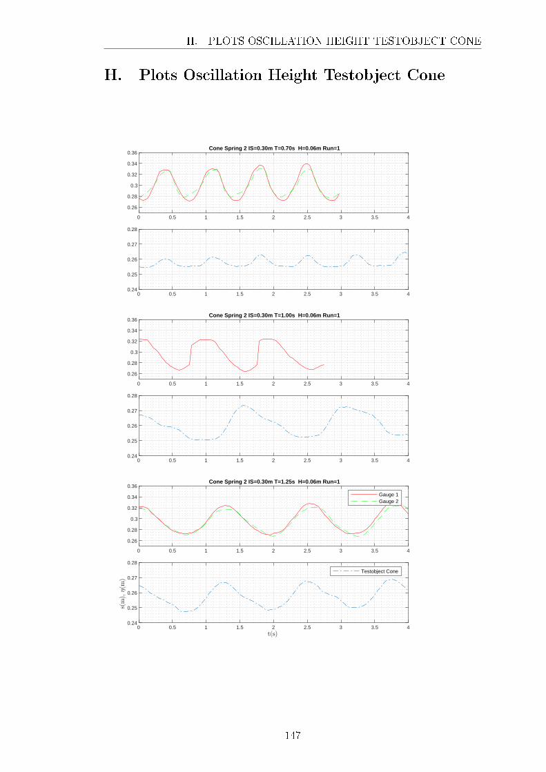
0 0.5 1 1.5 2 2.5 3 3.5 4
0.26
0.28
0.3
0.32
0.34
0.36 Cone Spring 2 IS=0.30m T=0.70s H=0.06m Run=1
0 0.5 1 1.5 2 2.5 3 3.5 40.24
0.25
0.26
0.27
0.28
0 0.5 1 1.5 2 2.5 3 3.5 4
0.26
0.28
0.3
0.32
0.34
0.36 Cone Spring 2 IS=0.30m T=1.00s H=0.06m Run=1
0 0.5 1 1.5 2 2.5 3 3.5 40.24
0.25
0.26
0.27
0.28
0 0.5 1 1.5 2 2.5 3 3.5 4
0.26
0.28
0.3
0.32
0.34
0.36 Cone Spring 2 IS=0.30m T=1.25s H=0.06m Run=1
Gauge 1Gauge 2
0 0.5 1 1.5 2 2.5 3 3.5 40.24
0.25
0.26
0.27
0.28
Testobject Cone
H. PLOTS OSCILLATION HEIGHT TESTOBJECT CONE
H. Plots Oscillation Height Testobject Cone
147
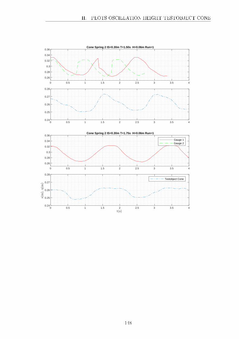
0 0.5 1 1.5 2 2.5 3 3.5 4
0.26
0.28
0.3
0.32
0.34
0.36 Cone Spring 2 IS=0.30m T=1.50s H=0.06m Run=1
0 0.5 1 1.5 2 2.5 3 3.5 40.24
0.25
0.26
0.27
0.28
0 0.5 1 1.5 2 2.5 3 3.5 4
0.26
0.28
0.3
0.32
0.34
0.36 Cone Spring 2 IS=0.30m T=1.75s H=0.06m Run=1
Gauge 1Gauge 2
0 0.5 1 1.5 2 2.5 3 3.5 40.24
0.25
0.26
0.27
0.28
Testobject Cone
H. PLOTS OSCILLATION HEIGHT TESTOBJECT CONE
148

0 0.5 1 1.5 2 2.5 3 3.5 4
0.26
0.28
0.3
0.32
0.34
0.36 Cone Spring 2 IS=0.27m T=0.70s H=0.06m Run=1
0 0.5 1 1.5 2 2.5 3 3.5 40.22
0.23
0.24
0.25
0.26
0 0.5 1 1.5 2 2.5 3 3.5 4
0.26
0.28
0.3
0.32
0.34
0.36 Cone Spring 2 IS=0.27m T=1.00s H=0.06m Run=1
0 0.5 1 1.5 2 2.5 3 3.5 40.22
0.23
0.24
0.25
0.26
0 0.5 1 1.5 2 2.5 3 3.5 4
0.26
0.28
0.3
0.32
0.34
0.36 Cone Spring 2 IS=0.27m T=1.25s H=0.06m Run=1
Gauge 1Gauge 2
0 0.5 1 1.5 2 2.5 3 3.5 40.22
0.23
0.24
0.25
0.26
Testobject Cone
H. PLOTS OSCILLATION HEIGHT TESTOBJECT CONE
149

0 0.5 1 1.5 2 2.5 3 3.5 4
0.26
0.28
0.3
0.32
0.34
0.36 Cone Spring 2 IS=0.27m T=1.50s H=0.06m Run=1
0 0.5 1 1.5 2 2.5 3 3.5 40.22
0.23
0.24
0.25
0.26
0 0.5 1 1.5 2 2.5 3 3.5 4
0.26
0.28
0.3
0.32
0.34
0.36 Cone Spring 2 IS=0.27m T=1.75s H=0.06m Run=1
Gauge 1Gauge 2
0 0.5 1 1.5 2 2.5 3 3.5 40.22
0.23
0.24
0.25
0.26
Testobject Cone
H. PLOTS OSCILLATION HEIGHT TESTOBJECT CONE
150