bachelor thesis: econometrics and operational research
TRANSCRIPT

ERASMUS UNIVERSITY ROTTERDAM
Erasmus School of Economics
Bachelor Thesis: Econometrics and Operational Research
Three-stage MLR, ANN and MARSmodels for long-term hourly load
forecasting
Student name: Breukelen, L.W.F. van
Student ID number: 484757
Supervisor: Vermeulen, S.H.L.C.G.
Second assessor: Oorschot, J.A.
Date final version: 02/07/2020
Abstract Electric load forecasts are vital to ensure reliable power supply. Load forecasts are
especially important, since power storage capacity is small. This paper evaluates the performance
of MLR, ANN and MARS models for modelling relationships between the hourly load demand in
Luxembourg and seasonal patterns, calendar effects as well as weather and economic variables. ANN
and MARS models forecast the hourly load demand more accurately than the MLR model, which
performance is especially lower if the relationships between variables seem to be more complex.
Incorporating uncertain weather and economic variables in the models does not enhance long-term
out-of-sample forecasts, but the developed models are nevertheless useful in other applications.
The views stated in this thesis are those of the author and not necessarily those of the supervisor,
second assessor, Erasmus School of Economics or Erasmus University Rotterdam.

Contents
1 Introduction 1
2 Literature 3
3 Data 6
4 Methodology 9
4.1 Multiple Linear Regression (MLR) . . . . . . . . . . . . . . . . . . . . . . . . . . . . 10
4.2 Artificial Neural Network (ANN) . . . . . . . . . . . . . . . . . . . . . . . . . . . . . 10
4.3 Multivariate Adaptive Regression Splines (MARS) . . . . . . . . . . . . . . . . . . . 12
4.4 Double seasonal block bootstrap . . . . . . . . . . . . . . . . . . . . . . . . . . . . . 13
5 Explanatory variables 14
6 Results 16
7 Conclusion 20
8 Recommendations 20
9 Appendix 21
9.1 Additional results . . . . . . . . . . . . . . . . . . . . . . . . . . . . . . . . . . . . . . 21
9.2 Additional methodology . . . . . . . . . . . . . . . . . . . . . . . . . . . . . . . . . . 24
10 MATLAB code 28

1 INTRODUCTION
1 Introduction
Electric load forecasts are vital for a reliably electric power industry. The forecasts are crucial
for decision making in the energy sector. For day-to-day operations such as the determination of
production scheduling and energy allocation, but also for long-term decisions such as investments in
new facilities. In comparison with other industries, accurate forecasting models for electric load are
especially important since electrical energy cannot be massively stored using today’s technologies,
implying that demand and supply should (almost) match at every moment.
Although there is not a golden standard for classifying the range of load forecasts, Hong and
Fan (2016) use a classification with a cut-off horizon of two weeks. Forecasts till two weeks are
short-term load forecasts (STLF) and forecasts exceeding two weeks are long-term load forecasts
(LTLF). In the existing literature, the LTLF frequency is usually low and the constructed models
serve a single, very specific forecasting problem. We make a model for LTLF at intervals of an hour
instead. The advantage of our model is the applicability to different load forecasting problems such
as: investment decisions, operations and maintenance, transmission and distribution planning as
well as demand management. Moreover, the incorporation of high frequency explanatory variables
could also enhance forecasting performance. Hong, Wilson, and Xie (2013) conclude that the
classical approach for LTLF is often limited to the use of load and weather information occurring
with monthly or annual frequency. They find that the use of low resolution and infrequent data can
lead to inaccurate forecasts. The high frequency approach in this paper, which takes advantage of
hourly information, could therefore result in more accurate and defensible forecasts.
In the absence of statistical software packages in the early ages of load forecasting, an engineering
approach was developed to manually forecast the future load using charts and tables. The invention
of the computer led to an abundance of load forecasting models. Out of the abundance of methods,
we use Multiple Linear Regression (MLR), Artificial Neural Network (ANN) and Multivariate
Adaptive Regression Splines (MARS) as in Nalcaci, Ozmen, and Weber (2019). The well-known
MLR and ANN have extensively been used for load forecasting purposes. Nalcaci et al. (2019) find
the performance of the relative uncommonly used MARS model competitive with the ANN model
for LTLF, which gives us reason to further investigate the performance of the MARS model.
The goal of this paper is to obtain a method suitable for making LTLF for all long-term forecast-
ing horizons up to three years after the forecast construction date. In order to prevent a look-ahead
bias, we only incorporate information which was available on the forecast construction date.
1

1 INTRODUCTION
Out of existing literature, Hong et al. (2010) conclude that weather variables, past load, calendar
events, and seasonal factors have a significant impact on the load demand. Past load is especially
informative for STLF, however becomes increasingly inaccurate if the forecasting horizon increases.
Due to the increasing inaccuracy for forecasts further away from the day at which the forecasts are
constructed, the use of past load is excluded from our models.
The relationships between the remaining explanatory variables and the load demand can either
be modelled in a single-stage model or by a sequence of stages. This paper uses a sequence of three
stages, since single-stage models can fail to incorporate multiple types of effects on the load demand
simultaneously. Zhang and Qi (2005) state that just as traditional statistical models, ANN is for
example not able to simultaneously model many different relationships between the explanatory
variables and dependent variable well. In the multi-stage models, the division is commonly based
on the type of phenomena which is modelled. Magnano and Boland (2007) for instance, start
with modelling the relationship between the load demand and the seasonal patterns, after which
they investigate the relationship between the season-adjusted load and weather variables. In our
sequence of three stages, the first stage removes the effect of seasonal patterns on the load demand.
The second stage investigates the relationship between the deseasonalized load and other calendar
events due to national holidays and vacation periods. These calendar events are separated from
the seasonal pattern, since it allows us to separately focus on the dominant and complex seasonal
patterns before incorporating other effects. Finally, the third stage investigates the relationship
between the season- as well as calendar-adjusted load and the weather and economic variables.
Since weather and economic variables are unknown for long periods ahead and we want to prevent
a look-ahead bias, double seasonal block bootstrap helps constructing different input scenarios. The
set of input scenarios leads to a set of forecasts. The average of the set of forecasts results in a
single time-series of LTLF, which is the final estimate of the three-stage model.
In summary, this paper investigates the performance of the MLR, ANN and MARS models
for LTLF in three consecutive stages, to find the best performing combination of these models.
Moreover, we investigate if bootstrap constructed uncertain explanatory variables could enhance
the out-of-sample forecasts. This leads to the following research question: What combination of
MLR, ANN and MARS models provide the most accurate hourly long-term load forecasts, when
applying three consecutive stages?
2

2 LITERATURE
The European Network of Transmission System Operations for Electricity (ENTSO-E) provides
the hourly load data from 01/01/2006 until 31/12/17 for the Grand-Duchy of Luxembourg. Methostat
provides the hourly weather data representative for Luxembourg. The measure for the state of the
economy is the DAX-index, which Yahoo! Finance provides. The data from 01/01/2006 until
31/12/14 is for construction of the three-stage models. These models are evaluated on the test
data, which starts at 01/01/2015 and ends at 31/12/17.
We implement the methods and models in MATLAB R2020a, extended with the Optimisation
and Deep Learning Toolbox as well as the MARS/ARESlab Toolbox of Jekabsons (2016). The
performance of the resulting models indicates that ANN and MARS models outperform the MLR
model, especially if the relationship between the explanatory variables and the dependent variable
seems to be more complex. In contrast to the MLR model, the ANN and MARS models find useful
functional relationships between weather and economic variables and the load demand which is ad-
justed for seasonal patterns and calendar effects. These relationships can be utilized for applications
such as ’what-if’ analyses, but are unable to enhance the out-of-sample forecast performance.
2 Literature
Load forecasting models can be divided in two groups (Hong & Fan, 2016). The first group consists
of statistical models, which is further divided into: multiple linear regression (MLR) models, auto-
regressive and moving average models, semi-parametric additive models and exponential smoothing
models. According to Hinman and Hickey (2009) and Nalcaci et al. (2019), the regression models
are widely used in electric load forecasting. The term ’regression’ in MLR refers to statistical pro-
cess for estimating the relationships among variables and the term ’linear’ to the linear equations
that are used to solve the parameters, rather than the relationships between the dependent and
independent variables (Hong & Fan, 2016). A MLR model distinguishes itself from a single linear
regression model, through the use of multiple explanatory variables instead of a single explanatory
variable. The advantage of the MLR model is that it is easy to interpret, implement and use.
Nalcaci et al. (2019) conclude however that the forecasts of MLR are less accurate in comparison
with alternative load forecasting models. A possible explanation is given by Metaxiotis, Kagian-
nas, Askounis, and Psarras (2003), which state that misspecification of the functional relationship
between the dependent and explanatory variables often is the cause of bad performance.
3

2 LITERATURE
The second group of load forecasting models consists of artificial intelligence (AI) based
models. AI is a relatively new research field, where common load forecasting methods include
neural networks, fuzzy regression models, support vector machines and gradient boosting machines.
Rosenblatt (1962) describes the usefulness of neural networks for many applications such as model
classification and learning methods. Neural networks are generally used for complex data structure
applications such as high-dimensional input data applications. By learning patterns from the his-
torical data, without requiring the forecaster to describe a functional relation between the input
(explanatory) and output (dependent) variables, a mapping between input and output is construc-
ted. AI models are better in dealing with non-linearity and other difficulties than statistical models,
since they do not require any complex mathematical formulation or quantitative correlation between
inputs and outputs (Metaxiotis et al., 2003). A disadvantage of AI methods is however that the
resulting mapping between input and output lacks the possibility of interpretation, which is reason
for Cevik et al. (2017) to see the behaviour of ANN as a ’black box’ model.
Many types of neural networks are used for load forecasting, such as feed-forward neural net-
works, radial basis function networks, and recurrent neural networks. An ANN is a feed-forward
neural network based on the biological brain, in which different layers of nodes (neurons) are connec-
ted by a network of weights (synapses). The weights and input variables, determine the output or
estimate of the model. To improve the forecasts accuracy, the weights are adjusted through an iter-
ative supervised training process. Rumelhart, Hinton, and Williams (1986) use backpropagation to
train a neural network. Hagan and Menhaj (1994) incorporate the Levenberg-Marquardt algorithm
(Marquardt, 1963) into the backpropagation algorithm for training feed-forward neural networks
and obtain more efficient results for small neural networks, compared to the backpropagation of
Rumelhart et al. (1986).
In practice, the boundary between statistical and AI models is quite ambiguous. MARS can
for instance belong to either of the two groups. MARS, as introduced by Friedman (1991), is a
non-parametric regression based method which is able to automatically model non-linearity’s and
interactions between variables. MARS consist of a forward and backward phase. In the forward
phase, the model is built. The built model is simplified in backward phase to prevent overfitting
of the model on the training data. In contrast to MLR but similar to the ANN, MARS has the
advantage that it does not need an assumption about the underlying functional relation between
dependent and independent variables. Nalcaci et al. (2019) find the performance of the MARS
superior to MLR models and competitive with the ANN for load forecasting. Since ANN and
4

2 LITERATURE
MARS are non-parametric methods that do not need a pre-specified functional relation, both the
model and the parameters need to be fitted on the training data. To prevent the non-parametric
methods to lack power, a large part of our data is dedicated to training the models.
Load forecasting models can consist of a single stage or a sequence of stages. Advantages of a
single-stage model are: all variables can interact, the model is simple to construction and the model
is easy to use for forecasting. A multi-stage approach, also called a multi-model approach, has the
advantage that the strengths of different methods can be combined to improve the forecast perform-
ance. Nelson, Hill, Remus, and O’Connor (1999) show the usefulness of multi-stage modelling for
neural networks on load data. In contrast to the theory that the non-parametric method should be
able to capture the (non-)linear seasonal pattern and weather information simultaneously, they find
the forecasts of neural networks to be significantly more accurate if the data is deseasonalized before
the relation with the weather variables is modelled. In later research, Zhang and Qi (2005) also
conclude: ”... just as traditional statistical models, neural networks are not able to simultaneously
handle many different components of the data well and hence data preprocessing is beneficial”.
Palit and Popovic (2006) state that the data preprocessing, or decomposition analyses of a
time-series usually consists of detrending and deseasonalizing the data. If the load demand contains
a significant trend or seasonal pattern, first removing the trend or seasonal pattern can simplify
modeling and improve model performance. After detrending the data, seasonality is a dominant
feature in the load demand time-series. Park, El-Sharkawi, Marks, Atlas, and Damborg (1991)
and Lusis, Khalilpour, Andrew, and Liebman (2017) observe that the hourly time-series for load
data contains daily, weekly and yearly seasonal patterns. There are various methods to deseason
the hourly load data. Chen, Wang, and Huang (1995) use subsets of data and then estimate the
parameters on each subset separately. The disadvantage of splitting the data into subsets is that it
can lead to an abundance of models. An alternative method to model seasonal patterns is the use
of explanatory variables. Hong et al. (2010) differentiate times of the day, week and year through
dummy variables, which are equal to one on specific moments of the day, week or year and zero
otherwise. Magnano and Boland (2007) use dummy variables to model the weekly seasonality,
however use polynomial Fourier series for modeling the daily and yearly seasonal patterns in the
load demand.
5

3 DATA
Besides a trend and seasonal pattern, Hong et al. (2010) conclude that national holidays, vacation
periods as well as weather and economic variables impact the load demand. On a national holiday
for instance, businesses, factories, and office buildings are mostly closed. Hong et al. (2010) find
that the effect of a national holiday in the US is comparable with the effect of either a Monday,
Saturday or Sunday. Due to a strong correlation between power consumption and weather variables
such as temperature, humidity, wind speed, and cloud cover, Park et al. (1991) conclude that
utilizing weather information can improve the accuracy of the forecasts. In contrast to Park et
al. (1991), Magnano and Boland (2007) find that weather variables have little explanatory power.
The difference in conclusions can be explained by the different moments of incorporation of the
weather data as explanatory variable. Park et al. (1991) use weather data directly as explanatory
variable for load demand, in contrast to Magnano and Boland (2007), who investigate the relation
between deseasonalized load and weather variables. The model for deseasonalizing the load data
already explains a significant amount of the variability of the electricity demand due to the weather
variables, after which the explanatory power of the weather variables itself, is far smaller.
Since weather and economic variables are uncertain in the long-term and we want to prevent
a look-ahead bias, the weather and economic variables are simulated. An average of the previous
decades is however not defensible according to Hyndman and Fan (2009). This approach is not
defensible since an average temperature profile understates the peaks and does therefore not repres-
ent the normal spread in weather. A second reason why the average weather profile may not lead
to a representative load profile is due to the non-linear relationship between the load and weather
variables. The solution of Hyndman and Fan (2009) is to use a double seasonal block bootstrap
method, which captures the daily as well as annual seasonality of the weather variables, to generate
more realistic input scenarios.
3 Data
The hourly load data in megawatt (MW ) for Luxembourg is freely accessible from the European
Network of Transmission System Operators for Electricity (ENTSO-E). ENTSO-E represents 42
electricity transmission system operators from 35 countries across Europe. Creos Luxembourg is
the transmission system operator which provides the data for the Grand-Duchy of Luxembourg.
Compared to other European countries, the load data of Luxembourg has the following advantages:
the ENTSO-E network is the single power provider for all of Luxembourg; the data collection
6
3 DATA
method has not changed over time and a single weather station is representative for the entire
country because Luxembourg is the second smallest country of Europe with a surface of only 2586
km2.
The load dataset starts at 0 AM 01/01/2006 local time and consists of hourly observations until
12 PM 31/12/2017, resulting in a period of 12 years, 4383 days or 105192 hours of data. 10 of the
105192 hourly load observations are missing, for which the average of the previous and next known
load is assumed. The data is split into a training and test set. The data for model construction is
the training set, which starts at 0 AM 01/01/2006 and ends at 12 PM 31/12/2014 (78888 hours).
LTLF are made and assessed against the test data, which starts at 0 AM 01/01/2015 and ends at
12PM 31/12/2017 (26304 hours). Although more accurate weather forecasts for the first two weeks
would have been available, this data is ignored in order to simulate identical data availability. This
allows us to make forecasts for these first two weeks, as if it were LTLF.
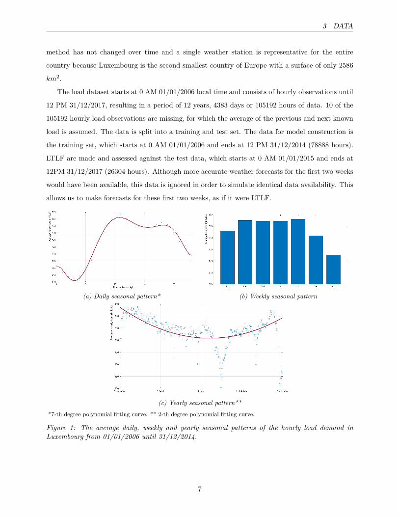
(a) Daily seasonal pattern* (b) Weekly seasonal pattern
(c) Yearly seasonal pattern***7-th degree polynomial fitting curve. ** 2-th degree polynomial fitting curve.
Figure 1: The average daily, weekly and yearly seasonal patterns of the hourly load demand inLuxembourg from 01/01/2006 until 31/12/2014.
7

3 DATA
The hourly load demand in Luxembourg contains daily, weekly and yearly seasonal patters.
Figure 1a shows the average load demand at different hours of the day for the training data. The
load demand is the lowest between midnight and 5 AM, after which the demand increases until
approximately 10 AM. The average demand is maximal between 10 AM and 8 PM, after which it
starts to decline. Figure 1b shows the weekly seasonal pattern, in which the average load demand
on Monday, Saturday and Sunday is lower than on the other days of the week. The yearly seasonal
pattern in Figure 1c shows that the average load demand is higher during winter months than
during summer months. Spring and Autumn fall in between these periods of high and low average
load demand.
The lines fitting the data in Figure 1a and 1c are 7-th and 2-th degree polynomial functions.
These polynomial functions serve as explanatory variables (Section 5) and the degree of these
polynomials is preferred over other polynomial degrees based on the fit of the average load demand
and the cyclical nature of the function, with a small difference between the load value at start and
end of a cycle. Since the explanatory variables for the weekly seasonal pattern consist of dummy
variable instead of polynomial functions, Figure 1b represents the weekly seasonality in a bar chart
instead.
The average load demand is lower on national holidays. The negative outlying observations
in Figure 1c are mainly the consequence of national holidays and vacation periods. The lower
demand at the end of December and at the beginning of January may be explained by Christmas
season. The demand decrease from mid- July until the end of August could be the result of summer
vacations and the construction break. The impact of national holidays is illustrated by the outlying
observation on 1 November, due to All Saints’ Day and the lower demand on 23 June, which is
the consequence of National Day. The reduction in load demand on the days surrounding national
holidays could be the result of extended holiday activities (Hong et al., 2010).
Meteostat provides the hourly weather data and is freely online accessible for high-frequency data
on weather and climate statistics worldwide. The only weather station in the Meteostat database
in Luxembourg is at Luxembourg Airport. Since this station contains many missing values and
has no hourly data for 2011, the closest weather station in Trier-Petrisberg (Germany) is used.
Trier-Petrisberg is roughly 10 km from the border of Luxembourg and 50 km from the city-centre of
Luxembourg. The hourly weather data consist of: the temperature (in ◦C), the dew point (in ◦C),
relative humidity (in %), precipitation (in mm), the wind speed (in km/h) and the air pressure (in
hPa) (Appendix 9.1.1). The amount of missing values for the weather variables is between 0.041
8

4 METHODOLOGY
and 0.165 percent, for which an average of the two adjacent observations is assumed. We expect
the influence of the missing load and weather values to be negligible, since the amount of missing
values is small and both time-series are continuous for which an average of adjacent data points
provides an reasonable approximation.
Yahoo! Finance provides an economic metric for Luxembourg, which is the DAX-index. The
DAX-index consists of 30 major German companies. The DAX-index provides a good measure
for economy of Luxembourg because Luxembourg’s economy is highly dependent on the economy
of Germany. German Federal Foreign Office (2020) state that Germany is Luxembourg’s main
economic partner, accounting for approximately 27% of total foreign trade in 2016.
4 Methodology
The first-stage model starts with modelling seasonal patterns, after which calendar events are in-
corporated in the second stage. In the last stage, the remaining effects of economic and weather
variables are modelled. The first stage model is given by Y1 = f(X1) +Y2, in which Y1 is the hourly
load demand and X1 consists of the explanatory variables to model seasonal patterns. The residuals
from the first stage (Y2) represent the deseasonalized load and are the dependent variable in the
second stage. The second stage removes the effects of national holidays and vacation periods (X2)
from the deseasonalized load, given by Y2 = g(X2)+Y3. In the third stage investigates the relation-
ship between weather and economic variables (X3) and the residuals from the second model (Y3).
This third and last stage model is given by Y3 = z(X3) + ε, in which ε represents the unexplained
variation of the load demand due to randomness and other, overlooked variables. The functions
f(.), g(.) and z(.) in the sequence of three stages are all estimated using MLR, ANN and MARS
models. The functions do not necessarily have to be constructed using the same model, such that
the strengths of different models in different stages can be combined.
The explanatory variables to model the effects of seasonal patterns and calendar effect are
known with certainty for the future, which we therefore directly use for out-of-sample forecasting.
Weather and economic variables are however uncertain in the long-term. By simulating different
input scenarios using double seasonal block bootstrap and averaging the resulting set of forecasts,
we construct out-of-sample point forecasts.
9

4.1 Multiple Linear Regression (MLR) 4 METHODOLOGY
4.1 Multiple Linear Regression (MLR)
A simple linear regression has a single explanatory variable, in contrast to MLR which has multiple
explanatory variables. The MLR model is given by Y = Xβ + ε, in which Y is a Tx1 vector of
the dependent variable, ε is a Tx1 vector of the residuals and the TxK matrix X contains for each
of the T data observations, the value of K explanatory variables. The coefficients in the Kx1 β
vector are estimated by Ordinary Least Squares (OLS) and measure the effect of each explanatory
variable after taking the effects of the other predictors into account.
The effect of a predictor variable may depend on the value(s) of some other predictor variable(s).
Nalcaci et al. (2019) use a MLR model which does not allow for interaction between the explanatory
variables. Since we expect the variables to be interacting and possibly non-linear, we use a simple
and an extended MLR model. The explanatory variable in the simple model consists of only
an intercept term and non-interacting linear explanatory variables. The extended MLR contains,
besides the intercept term and the non-interacting linear explanatory variables, squared terms as well
as interacting terms, which consist of the product of two distinct predictors. Based on the AIC-
criteria, we add explanatory variables using forward selection, after which backward elimination
investigates if some of the variables can be removed due to a lack of explanatory power.
4.2 Artificial Neural Network (ANN)
ANN is a neural network based on a biological brain, which can model complex and possibly non-
linear relationships between the dependent output variable Y and the K explanatory input variables
in X, given by Y = h(X) + ε.
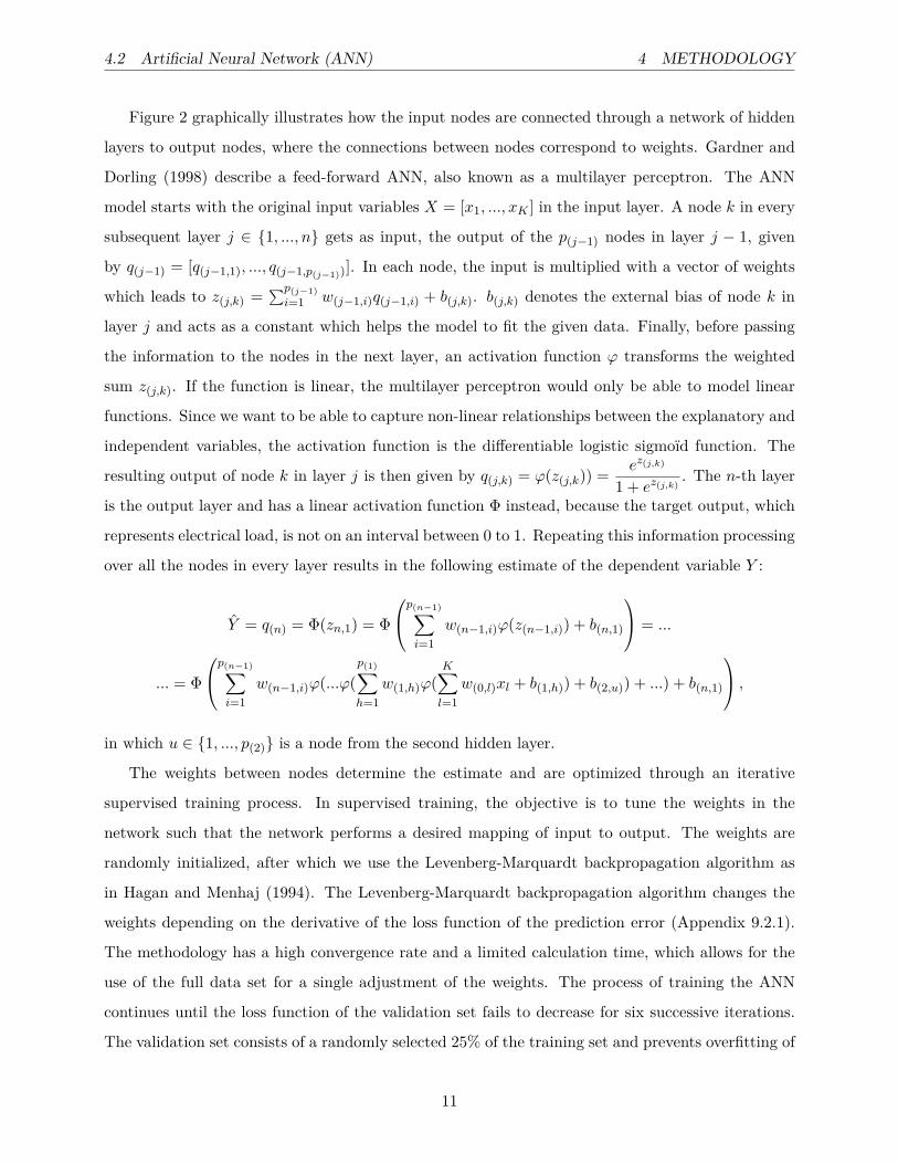
Figure 2: A scheme for the ANN.
10
4.2 Artificial Neural Network (ANN) 4 METHODOLOGY
Figure 2 graphically illustrates how the input nodes are connected through a network of hidden
layers to output nodes, where the connections between nodes correspond to weights. Gardner and
Dorling (1998) describe a feed-forward ANN, also known as a multilayer perceptron. The ANN
model starts with the original input variables X = [x1, ..., xK ] in the input layer. A node k in every
subsequent layer j ∈ {1, ..., n} gets as input, the output of the p(j−1) nodes in layer j − 1, given
by q(j−1) = [q(j−1,1), ..., q(j−1,p(j−1))]. In each node, the input is multiplied with a vector of weights
which leads to z(j,k) =∑p(j−1)i=1 w(j−1,i)q(j−1,i) + b(j,k). b(j,k) denotes the external bias of node k in
layer j and acts as a constant which helps the model to fit the given data. Finally, before passing
the information to the nodes in the next layer, an activation function ϕ transforms the weighted
sum z(j,k). If the function is linear, the multilayer perceptron would only be able to model linear
functions. Since we want to be able to capture non-linear relationships between the explanatory and
independent variables, the activation function is the differentiable logistic sigmoıd function. The
resulting output of node k in layer j is then given by q(j,k) = ϕ(z(j,k)) = ez(j,k)
1 + ez(j,k). The n-th layer
is the output layer and has a linear activation function Φ instead, because the target output, which
represents electrical load, is not on an interval between 0 to 1. Repeating this information processing
over all the nodes in every layer results in the following estimate of the dependent variable Y :
Y = q(n) = Φ(zn,1) = Φ
p(n−1)∑i=1
w(n−1,i)ϕ(z(n−1,i)) + b(n,1)
= ...
... = Φ
p(n−1)∑i=1
w(n−1,i)ϕ(...ϕ(p(1)∑h=1
w(1,h)ϕ(K∑l=1
w(0,l)xl + b(1,h)) + b(2,u)) + ...) + b(n,1)
,in which u ∈ {1, ..., p(2)} is a node from the second hidden layer.
The weights between nodes determine the estimate and are optimized through an iterative
supervised training process. In supervised training, the objective is to tune the weights in the
network such that the network performs a desired mapping of input to output. The weights are
randomly initialized, after which we use the Levenberg-Marquardt backpropagation algorithm as
in Hagan and Menhaj (1994). The Levenberg-Marquardt backpropagation algorithm changes the
weights depending on the derivative of the loss function of the prediction error (Appendix 9.2.1).
The methodology has a high convergence rate and a limited calculation time, which allows for the
use of the full data set for a single adjustment of the weights. The process of training the ANN
continues until the loss function of the validation set fails to decrease for six successive iterations.
The validation set consists of a randomly selected 25% of the training set and prevents overfitting of
11

4.3 Multivariate Adaptive Regression Splines (MARS) 4 METHODOLOGY
the ANN model. Since the number of training observations is large and we use 25% of the training
data as validation set, we do not add more restriction to the validation set.
The best method to set the number of nodes and hidden layers is testing different settings, since
Karsoliya (2012) finds the tuning of these parameters problem specific, such that no general best
setting is available. We found it optimal in our models to set the number of hidden layers at two
and the number of nodes per hidden layer at fifteen. Smaller neural networks are less accurate, but
neural networks with more nodes do not improve the forecasts accuracy significantly and can result
in overfitting.
4.3 Multivariate Adaptive Regression Splines (MARS)
Friedman (1991) introduces the MARS method, which is a generalization of a linear step-wise
regression. MARS models the relationship between the dependent variable Y and the explanatory
variables in the matrix X = [x1, ..., xK ] in the following form: Y = b(X) + ε. The estimation of
the b(.) function is b(X) =∑Mi=1 ciBi(X), in which ci is the coefficient corresponding to the basis
function Bi(X). The coefficient is determined using OLS and a basic function is either a constant
or a (product of) hinge function(s). A hinge function, also known as a two-sided truncated power
basis (Friedman, 1991), is given by [±(xj − τj)]+, in which the + symbol specifies that only the
positive parts are used. [(x− τ)]+ can therefore be rewritten as max{0, x− τ} and [−(x− τ)]+ as
max{0, τ − x}. A basis function has the following form Bi(X) = ΠKij=1[±(xj − τj)]+, in which Ki
represents the number of variables involved in the i-th basis function and τj is a knot. A knot is a
point on the domain of a variable, where the ±-sign in the hinge function switches from positive to
negative or vice versa (Appendix 9.2.2, Figure 5).
MARS implements a sequence of two phases, namely a building and backward phase. In the
building phase, the estimated function starts with only a single basis function which consist of a
constant (b(X) = c0). This function is then repeatedly extended with a pair of basis functions
until the maximum of basis functions is reached (M = Mmax) or the Generalized Cross-Validation
(GCV) has not decreased significantly. GCV is a performance measure for the MARS model, which
depends on the model complexity µ. The GCV (µ) is given by:
T∑t=1
(yt − fµ(xt))2
(1−M(µ)/T )2 ,
in which M(µ) represents the effective number of parameters and is calculated as M(µ) = u+d×λ.
12

4.4 Double seasonal block bootstrap 4 METHODOLOGY
Here, u represent the number of basis functions, λ is the number of knots and d represent the cost
for each extra knot. Under the assumption that M(µ) < T and that all other components stay
the same, a higher M(µ) corresponds to a more complex model and therefore a higher GCV. In
each iteration, MARS adds the pair of basis functions which leads to the maximum reduction in
GCV. A pair of basis functions, instead of a single basis function, is added because both parts of
the hinge function ([+(xj − τj)]+ and [−(xj − τj)]+) are multiplied with one of the basis functions
in the model. The new hinge function depends on which knot locations are allowed per variable.
To reduce computation time and to lower the local variance of estimates, only a subset of knot
locations in the domain of a variable is considered (Appendix 9.2.2). After the building phase, we
apply a backwards stepwise procedure as in Friedman (1991) to prevent overfitting by decreasing
the complexity while maintaining a relative good fit. In the backward phase, MARS deletes the
single basis function which maximizes the decrease in GCV and continues as long as the decrease
in GCV is significant.
The cost of extra knots (d) is set at 3, which lies in the middle of the [2,4] interval which
Friedman (1991) advises. Moreover, the maximum number of basis functions in the forward phase
(Mmax) should be approximately twice the amount of nodes in the model with the lowest GCV.
The maximum allowed number of basis function in the forward phase is therefore set at 100. The
maximum number of interacting hinge functions is 3, which we find the best compromise between
the fit of the data on the one hand and simplicity and calculation time on the other hand.
4.4 Double seasonal block bootstrap
Bootstrapping involves random re-sampling of historical data. Block bootstrap aims to replicate the
correlation in the data by re-sampling blocks of data instead of individual data points. Hyndman
and Fan (2009) state that it is important to preserve any seasonal or trend patterns as well as
inherent serial correlation. The weather data contains no unidirectional trend but it contains a
daily and yearly seasonal pattern (Appendix 9.1.1). To preserve both the daily and yearly seasonal
pattern, we use a variant of the double seasonal block bootstrap of Hyndman and Fan (2009) and
combine the sampled blocks of data to generate one long input scenario.
13

5 EXPLANATORY VARIABLES
The length of each block is a multiple of the length of the daily seasonal period. Each block
consist of α whole days or α ∗ 24 hourly observations to preserve the daily pattern. To preserve
the yearly pattern, blocks in the generated input scenario start on the same day of the year as the
historical data or ±λ days, where λ is an independent uniformly distributed integer in the interval
[-14,14]. To divide each year in 4 blocks, α is 91 or 92 days. Blocks of this length are long enough to
capture serial correlations within these blocks, however short enough to allow sufficient series to be
generated. Moreover, the amount of unrealistically large jumps between blocks in the new scenario
is small, which should prevent the jumps to impact the forecast performance significantly.
5 Explanatory variables
Stage 1: Seasonal patterns
The load demand in Luxembourg contains no clear increasing or decreasing trend over the years,
so a trend correction is not needed. Therefore, the hourly load demand is only deseasonalized. The
seasonality in the hourly load demand consist of a daily, weekly and yearly seasonal pattern (Section
3). Based on in-sample performance and autocorrelation in the residuals, different combinations of
dummy and polynomial variables are evaluated. The resulting explanatory variables in the first-
stage models consist of: a constant, two polynomial terms and three dummy variables.
The standardized 7-th degree polynomial from Figure 1a captures the daily seasonal pattern.
The standardized quadratic trend-line from Figure 1c is the second explanatory polynomial variable
and captures the yearly seasonal pattern. The three dummy variables differentiate different days
of the week. Monday, Saturday and Sunday each get a separate dummy variable, which is equal to
one on the specific day of the week and zero otherwise. We choose to include variables for Monday,
Saturday and Sunday specifically, because Figure 1b shows that the average load demand on these
days is lower compared to the remaining days of the week.
Stage 2: National holidays and vacation periods
Hong et al. (2010) compare the effect of a national holiday in the United States to either a
Saturday, Sunday or Monday. We use dummy variables instead, because Luxembourg has different
national holidays than the United States and it does not require potentially inaccurate assumptions
about which weekday is comparable to which national holiday. In the second-stage, each of the
following extraordinary days are separated from the ordinary days with a dummy variable: national
14
5 EXPLANATORY VARIABLES
holidays, day before and after a national holiday, Christmas Season, peak summer and late summer.
The dummy to model the effect of national holidays is equal to one on: New Year, Easter, Labour
Day, Ascension Day, White Monday, National Day, Assumption Day, All Saints’ Day, Christmas
Day and Boxing Day. The specific dates of Christmas season differ each year, but are generally
speaking from the weekend before Christmas until the weekend after New Year. For the peak
summer, we use the construction break. Stopping construction affects consumption which reduces
power generation needs and it falls together with school vacations. Late or after summer starts
directly after the end of the peak summer and usually covers the last two weeks of August.
Even after deseasonalizing the load demand, the effect of extraordinary days can dependent on
the time of the year, day of the week and hour of the day. For instance, the effect of a national
holiday in a weekend can be smaller than on a weekday since many businesses were already closed.
Therefore, we include the two polynomial terms from the first-stage as well as a single dummy
to differentiate weekends from weekdays. A combination of time-dependent and calendar variables
can be informative. The time-dependent variables should have no explanatory power on themselves,
since these effects are already modelled in the first-stage model.
Stage 3: Weather and economic variables
The hourly weather data of the Meteostat database consist of: the temperature (in ◦C), the dew
point (in ◦C), precipitation (in mm), the wind speed (in m/s) and the air pressure in hectopascal
(hPa). Alongside the Meteostat variables, the set of explanatory weather variables consists of: the
maximum and minimum temperature in the last 24 hours, the difference between minimum and
maximum temperature in last 24 hours, an average temperature at the same time of a day over the
last seven days, precipitation in the last 24 hours, Heating Degree Day (HDD) and Cooling Degree
Day (CDD).
HDD and CDD are designed to quantify the demand for energy needed to heat or cool a build-
ing. They are defined relative to a base temperature, which is the outside temperature below or
above a building needing heating or cooling. European Environment Agency (2019) sets the base
temperature in the European Union at 15.5◦C and 22.0◦C respectively. If avg temp is the average
temperature in the last 24 hours, then HDD at a certain hour is max{0, 15.5 - avg temp} and CDD
is max{0, avg temp - 22.0}.
15

6 RESULTS
The economic explanatory variable in the third-stage model is the simple stock return of the
DAX-index over the last month. The stock return is more appropriate than the DAX-index itself,
since the models do not correct for the predominate upward trend of the DAX-index. The effect of
changing economic circumstances has a delayed effect on the load demand, which is reason to use
the stock return over an entire month. Lastly, the third-stage set of explanatory variables contains
the time-dependent variables from the second stage. The effects of weather variables on the season-
as well as calendar-adjusted load demand can dependent on the time. For instance, the effect of
a cold weekend day on which many people are at home, can differ from a cold weekday on which
most people are working.
6 Results
The first stage models the daily, weekly and yearly seasonal patterns in the hourly load demand.
Table 1 contains the forecast performance of the MLR, extended MLR with interacting and quad-
ratic terms, ANN and MARS models, in which the performance is based on the R2adj , RMSE and
MAPE forecasts criteria (Appendix 9.1, Table 6). Extending the MLR model with quadratic as
well as interacting terms, improves the forecast performance. The MAPE for the training data
reduces from 11.15% to 10.58% and the MAPE for the out-of-sample test dataset reduces from
11.14% to 10.76%. Compared to the (extended) MLR model, ANN and MARS models incorporate
more of the information contained in the explanatory variables for modelling seasonality. For the
training and test dataset, the R2adj is closer to one and both the RMSE and MAPE are closer to
zero. The MARS model is especially suitable for deseasonalizing the load demand, since it performs
best on all criteria.
Table 1: Forecasts performance of MLR, extended MLR, ANN and MARS models for modellingdaily, weekly and yearly seasonality in first stage. Training data from 01/01/2006 until 31/12/2014,test data from 01/01/2015 until 31/12/2017. The best performance is highlighted in bold.
MLR ext. MLR ANN MARS
Criteria Train Test Train Test Train Test Train Test
R2adj 0.431 0.292 0.479 0.329 0.573 0.383 0.608 0.455
RMSE 96.56 95.96 92.39 93.41 83.65 89.53 80.11 84.19MAPE (%) 11.15 11.14 10.58 10.76 9.57 10.32 9.19 9.59
16

6 RESULTS
Table 2 compares the training performance of the first-stage ANN and MARS models on ex-
traordinary days based on the average residual (Avg. Resid), RMSE and MAPE. The average
residuals are negative in vacation periods, on national holidays and on the days surrounding national
holidays. This indicates that the ANN and MARS model overestimate the load demand on the ex-
traordinary days, which is a consequence of the lower average load demand on these extraordinary
days (Section 3). On ordinary days the RMSE of the MARS model is 76.90, which increases on
extraordinary days to a minimum of 80.09 and maximum of 142.6. The ANN and MARS models
underestimate the load demand on ordinary days, which can be the result of the overestimation
on extraordinary days. Moreover, it is remarkable that the forecast errors of the ANN model on
extraordinary days are higher than of the MARS model.
Table 2: Forecasting performance on national holidays and in vacation periods for the first-stageANN and MARS models, 01/01/2006 until 31/12/2014.
ANN MARS ANN MARS ANN MARS
Criteria National holiday ± National holiday* Peak summer
Avg. Resid. (MW) -110.2 -81.04 -49.46 -19.59 -46.16 -46.15RMSE 152.0 142.6 111.0 93.20 79.38 80.09MAPE (%) 24.42 21.96 15.87 12.70 10.61 10.69
Holiday season Late summer Ordinary
Avg. Resid. (MW) -78.67 -22.76 -45.29 -37.92 11.75 8.16RMSE 122.0 94.43 81.25 80.97 79.20 76.90MAPE (%) 18.37 13.10 11.81 11.46 8.63 8.41
*Day before and day after national holidays.
Table 3: Forecasts performance of MLR, extended MLR, ANN and MARS models for modelling na-tional holidays and vacations in the second stage. Training data from 01/01/2006 until 31/12/2014,test data from 01/01/2015 until 31/12/2017. The best performance is highlighted in bold.
Stage 2: None* MLR Ext. MLR ANN MARSTrain Test Train Test Train Test Train Test Train Test
Stage 1: MARSR2adj 0.608 0.455 0.630 0.474 0.644 0.477 0.665 0.481 0.665 0.473
RMSE 80.11 84.19 77.89 82.69 76.40 82.47 74.10 82.13 74.12 82.74MAPE (%) 9.19 9.59 8.88 9.41 8.69 9.35 8.42 9.29 8.42 9.36Stage 1: ANNR2adj 0.573 0.383 0.619 0.432 0.633 0.442 0.678 0.472 0.674 0.470
RMSE 83.65 89.53 79.03 85.92 77.56 85.18 72.64 82.82 73.05 82.99MAPE (%) 9.57 10.32 8.96 9.79 8.76 9.66 8.23 9.40 8.30 9.40
*First-stage results from Table 1.
17
6 RESULTS
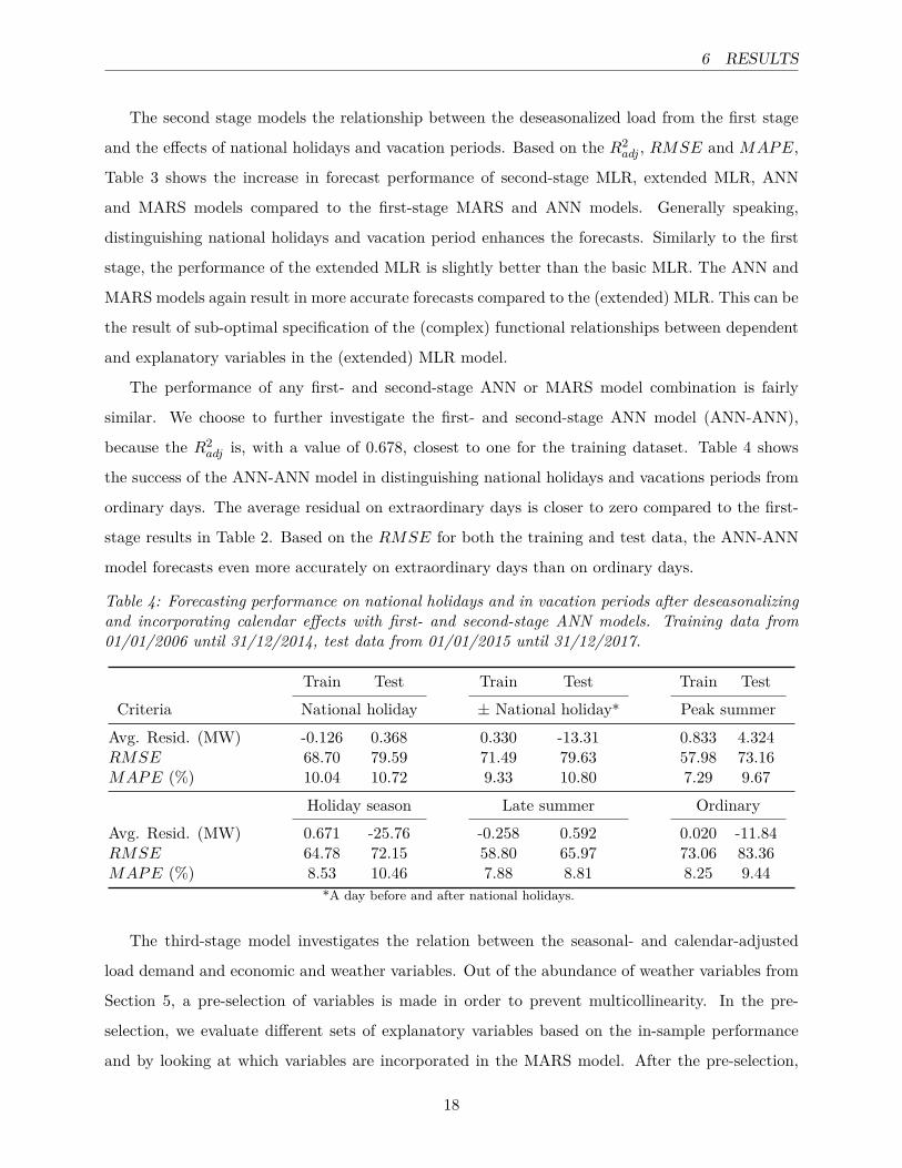
The second stage models the relationship between the deseasonalized load from the first stage
and the effects of national holidays and vacation periods. Based on the R2adj , RMSE and MAPE,
Table 3 shows the increase in forecast performance of second-stage MLR, extended MLR, ANN
and MARS models compared to the first-stage MARS and ANN models. Generally speaking,
distinguishing national holidays and vacation period enhances the forecasts. Similarly to the first
stage, the performance of the extended MLR is slightly better than the basic MLR. The ANN and
MARS models again result in more accurate forecasts compared to the (extended) MLR. This can be
the result of sub-optimal specification of the (complex) functional relationships between dependent
and explanatory variables in the (extended) MLR model.
The performance of any first- and second-stage ANN or MARS model combination is fairly
similar. We choose to further investigate the first- and second-stage ANN model (ANN-ANN),
because the R2adj is, with a value of 0.678, closest to one for the training dataset. Table 4 shows
the success of the ANN-ANN model in distinguishing national holidays and vacations periods from
ordinary days. The average residual on extraordinary days is closer to zero compared to the first-
stage results in Table 2. Based on the RMSE for both the training and test data, the ANN-ANN
model forecasts even more accurately on extraordinary days than on ordinary days.
Table 4: Forecasting performance on national holidays and in vacation periods after deseasonalizingand incorporating calendar effects with first- and second-stage ANN models. Training data from01/01/2006 until 31/12/2014, test data from 01/01/2015 until 31/12/2017.
Train Test Train Test Train Test
Criteria National holiday ± National holiday* Peak summer
Avg. Resid. (MW) -0.126 0.368 0.330 -13.31 0.833 4.324RMSE 68.70 79.59 71.49 79.63 57.98 73.16MAPE (%) 10.04 10.72 9.33 10.80 7.29 9.67
Holiday season Late summer Ordinary
Avg. Resid. (MW) 0.671 -25.76 -0.258 0.592 0.020 -11.84RMSE 64.78 72.15 58.80 65.97 73.06 83.36MAPE (%) 8.53 10.46 7.88 8.81 8.25 9.44
*A day before and after national holidays.
The third-stage model investigates the relation between the seasonal- and calendar-adjusted
load demand and economic and weather variables. Out of the abundance of weather variables from
Section 5, a pre-selection of variables is made in order to prevent multicollinearity. In the pre-
selection, we evaluate different sets of explanatory variables based on the in-sample performance
and by looking at which variables are incorporated in the MARS model. After the pre-selection,
18

6 RESULTS
the set of explanatory weather variables for Luxembourg consist of: HDD, precipitation in the last
24 hours, temperature and dew point.
Table 5 contains the third-stage forecast performance of the MLR, extended MLR, ANN and
MARS models using the season- and calendar adjusted load from the ANN-ANN model. The train-
ing performance of the third-stage (extended) MLR model has not improved significantly compared
to the second-stage ANN-ANN forecasts, which indicates that these methods do not find weather
and economic data informative. An explanation could be that the relationship between the already
adjusted load demand and the economic and weather variables is too complex for the (extended)
MLR model (Hyndman & Fan, 2009). In contrast to the (extended) MLR model, the third-stage
ANN and MARS models enhance the in-sample forecasts. The ANN-ANN model has a MAPE
of 8.23%, which the third-stage ANN and MARS models reduce to 6.49% and 6.96% respectively.
The total effect of the weather variables on the load demand is probably higher than incorporated
in the third-stage model, since a part of the effects of weather variables is already incorporated in
the first-stage deseasonalizing model (Magnano & Boland, 2007). If one is in possession of weather
data and the load demand is already adjusted for seasonality, we still recommend to incorporate
weather variables since the third-stage ANN and MARS models enhances the in-sample forecasts.
To deal with the uncertainty of weather and economic variables for out-of-sample LTLF, 1000
different scenarios are generated using double seasonal block bootstrap. Some of the 1000 input
scenarios improve the LTLF, however the use of the average of the 1000 different scenario forecasts
does not improve the LTLF performance (Table 5: Test data). The constructed three-stage ANN
and MARS models can however be useful for other application such as ’what-if’ analyses.
Table 5: Forecasting performance of MLR, extended MLR, ANN and MARS models in the thirdstage, where the relationship between economic and weather variables and the residuals from first-and second-stage ANN model is investigated. Training data from 01/01/2006 until 31/12/2014, testdata from 01/01/2015 until 31/12/2017. Estimates on the test data for the (extended) MLR areomitted, since the use of economic and weather variables do not improve model performance on thetraining data. The best training performance is highlighted in bold.
Target* MLR ext. MLR ANN MARS
Criteria Train Test Train Test Train Test Train Test Train Test
R2adj 0.678 0.472 0.681 - 0.684 - 0.797 0.466 0.766 0.471
RMSE 72.64 82.82 72.32 - 71.99 - 57.73 83.33 61.88 82.96MAPE (%) 8.23 9.40 8.19 - 8.14 - 6.49 9.45 6.96 9.41
*Forecasts from the ANN-ANN model (as in Table 3).
19

8 RECOMMENDATIONS
7 Conclusion
Electric load forecasts are vital to ensure reliable power supply. This paper investigates three-stage
Multiple Linear Regression (MLR), Artificial Neural Network (ANN) and Multivariate Adaptive Re-
gression Splines (MARS) models for hourly long-term load forecasting in Luxembourg. The hourly
long-term forecasts are suitable for many load forecasting problems such as: investment decisions,
operations and maintenance, transmission and distribution planning as well as demand manage-
ment. The explanatory variables incorporated in the three stages consist of: seasonal patterns,
calendar effects as well as weather and economic variables. In each stage, the non-parametric ANN
and MARS models result in more accurate forecasts in comparison to the parametric (extended)
MLR model, especially when the relation between variables seems to be more complex. In contrast
to the MLR method, ANN and MARS models are able to find functional relationships between
weather and economic variables on the one hand and seasonal- as well as calendar-adjusted load
on the other hand. The values of the economic and weather explanatory variables are however
unknown in the long-term. A set of 1000 weather and economic scenarios is generated, using double
seasonal block bootstrap. Each scenario leads to hourly forecasts for the entire test dataset. In con-
trast to some of the scenarios, the average of the 1000 load forecasts does not enhance the forecast
performance. The constructed three-stage models are however useful in other applications, such as
’what-if’ analyses.
8 Recommendations
Further research can investigate if a simplified model can be developed through merger of stages. An
example is to incorporate the seasonal, calendar, economic and weather patterns in a single stage.
The effect of the bootstrap generated economic and weather scenarios may then be able to enhance
the out-of-sample forecasts. New research can also investigate if the forecasts can be enhanced by
differentiating types of consumers. ENTSO-E serves different types of energy consumers such as
residents, businesses, and industries. Since effects of the explanatory variables on the energy demand
are likely to be consumer specific, a model dedicated to only one sector may enhance the forecast
performance. To prevent a look-ahead bias, we omitted past load as explanatory variable. The
influence on model performance by including past load as explanatory variable can be investigated,
possibly in combination with short- instead of long-term load forecasts.
20

9 APPENDIX
9 Appendix
9.1 Additional results
Table 6: Explanation of performance measures.
Name Explanation Goal Formula
Avg. Resid. Average residual Close to zero1T
∑Tt=1(yt − yt)
R2adj Percentage of explained variation Close to one 1−
( ∑Tt=1(yt − yt)2∑Tt=1(yt − yt)2
)(T − 1
T − p− 1
)
RMSE Square root of mean squared error Close to zero√
1T
∑Tt=1(yt − yt)2
MAPE Average magnitude of percentage errors Close to zero 1T
∑Tt=1
∣∣∣yt − ytyt
∣∣∣T represents the amount of observations and p corresponds with the number of parameters in a model.
Table 7: Performance of the first-stage ANN and MARS models on different times of the day, weekand year. Period: 01/01/2006 until 31/12/2014.
ANN MARS
Season Summer Winter Autumn Spring Summer Winter Autumn Spring
R2adj 0.582 0.550 0.556 0.524 0.583 0.679 0.560 0.512
RMSE 78.74 92.14 82.26 80.97 78.66 77.79 81.92 81.97
MAPE (in %) 9.59 10.17 9.55 9.00 9.53 8.57 9.52 9.11
Weekday Monday Saturday Sunday Rest Monday Saturday Sunday Rest
R2adj 0.610 0.340 0.305 0.496 0.635 0.368 0.278 0.553
RMSE 83.40 80.43 69.72 87.60 80.65 78.68 71.02 82.45
MAPE (in %) 9.65 9.42 9.38 9.64 9.30 9.23 9.44 9.08
Hours 0-6 6-12 12-18 18-24 0-6 6-12 12-18 18-24
R2adj 0.318 0.578 0.514 0.453 0.365 0.614 0.559 0.500
RMSE 81.96 83.98 84.14 84.49 79.07 80.32 80.22 80.83
MAPE (in %) 10.74 9.34 8.92 9.29 10.31 9.00 8.54 8.89
21

9.1 Additional results 9 APPENDIX
9.1.1 Seasonal patterns in weather data
(a) Temperature (b) Dew point
(c) Relative humidity (d) Wind speed
(e) Air pressure
Figure 3: Daily seasonal pattern of weather variables in Trier-Petrisberg based on average hourlydata, starting at 01/01/2006 and ending on 31/12/2014. Lines connect data points directly andprecipitation is omitted due to a lack of daily seasonal pattern.
22

9.1 Additional results 9 APPENDIX
(a) Temperature (b) Dew point
(c) Relative humidity (d) Wind speed
(e) Precipitation
Figure 4: Yearly seasonal pattern of weather variables in Trier-Petrisberg based on average dailydata, starting at 01/01/2006 and ending on 31/12/2014. Air pressure is omitted due to a lack ofyearly seasonal pattern.
23

9.2 Additional methodology 9 APPENDIX
9.2 Additional methodology
9.2.1 Levenberg-Marquardt backpropagation
In the Levenberg-Marquardt backpropagation algorithm of Hagan and Menhaj (1994), the loss
function of sum squared errors is given by V (w) =∑Ti=1 ε
2i (w) = ε′ε =
∑Ti=1(yt − yt)2, in which T
is the number of observations and V (w) is the loss function to minimize, with respect to the vector
w which contains n weights. As in quasi-Newton methods, the Levenberg-Marquardt algorithm
approximates the second-order derivative of the loss function instead of computing the real Hessian
matrix, which reduces the computation time. If J is the Jacobian matrix with the first derivatives
of the network error with respect to the weights and biases is given by
J(w) =
∂ε1(w)∂w1
. . . ∂ε1(w)∂wn
......
∂εN (w)∂w1
. . . ∂εN (w)∂wn
,
then the Hessian matrix is approximated by H = J ′J and the gradient is computed as g = J ′e.
After calculation of the gradient and approximation of the Hessian matrix, the weights in the
neural network are adjusted. The new weights are given by wnew = wold − [H + µI]−1g, in which
the scalar µ is a ’damping parameter’ which essentially determines the method used to update
the weights. If µ is large, the Levenberg-Marquardt backpropagation is essentially using gradient
descent. When µ ≈ 0, the algorithm uses the Gauss-Newton method to update the weights instead.
The ’damping parameter’ is initialized with a large value so the method starts with gradient descent.
Gradient decent updates the weights in the steepest-decent direction, without incorporating second
order derivatives. Gauss-Newton updates the weights by incorporating an estimate of the Hessian
matrix. The Gauss-Newton algorithm may converge slowly or not at all, if the initial guess is
far from the minimum or the Hessian matrix is ill-conditioned. Far away from the minimum,
the Levenberg-Marquardt method therefore acts more like a gradient-descent method. When the
parameters are close to their optimal value, the Levenberg-Marquardt method acts like the Gauss-
Newton method. After each iteration, µ is adjusted by either multiplying or dividing by β = 10.
When the loss function decreases, µ is divided by β and if a tentative step increases the loss function,
µ is multiplied by β.
24

9.2 Additional methodology 9 APPENDIX
9.2.2 Knot locations
In this paper, we use the knot placement algorithm of Friedman (1991). A knot placing algorithm
lowers the local variance of the estimates, which makes the method resistant to runs of positive
or negative error values between knots and it reduces the calculation time significantly. The knot
locations are determined for each variable individually and require a minimum number of observation
in between. The variance of the function estimates is especially high near the end of the domain of
a variable, due to the lack of constraints on the fit at the boundaries. The minimum observations
between the extreme knots and the corresponding interval ends are given by: 3− log2(αn ), in which
we set α = 0.05 and n denotes the total number of explanatory variables under investigation.
The minimum amount of observations for the remaining knots, which are in between the extreme
knots locations, is given by − log2(− 1nNm
ln(1 − α))/2.5, in which Nm is then number of positive
observations in the m-th basis function.
In the third-stage model, the minimum observations between two knots is set at 500 instead.
The knot placements in third-stage model needs to be adjusted, because the knot placement of
Friedman (1991) allows for too many knots locations, which results in unfeasible long computation
time. The first- and second-stage models do not need this adjustment, because a significant part of
the explanatory variables in these stages consists of dummy variables. Since dummy variables only
contain two values, the total number of knot location to evaluate remains feasible.
Figure 5: A mirrored pair of hinge functions with a knot at x=3.1.
25

REFERENCES REFERENCES
References
Cevik, A., Weber, G.-W., Eyuboglu, B. M., Oguz, K. K., Initiative, A. D. N., et al. (2017). Voxel-
MARS: a method for early detection of Alzheimer’s disease by classification of structural brain
MRI. Annals of Operations Research, 258 (1), 31–57.
Chen, J.-F., Wang, W.-M., & Huang, C.-M. (1995). Analysis of an adaptive time-series autoregress-
ive moving-average (ARMA) model for short-term load forecasting. Electric Power Systems
Research, 34 (3), 187–196.
European Environment Agency. (2019, Jun). Heating and cooling degree days.
Friedman, J. H. (1991). Multivariate adaptive regression splines. The annals of statistics, 1–67.
Gardner, M. W., & Dorling, S. (1998). Artificial neural networks (the multilayer perceptron)—a
review of applications in the atmospheric sciences. Atmospheric environment, 32 (14-15),
2627–2636.
German Federal Foreign Office. (2020, Jun). Germany and Luxembourg: Bilateral Relations.
Hagan, M. T., & Menhaj, M. B. (1994). Training feedforward networks with the Marquardt
algorithm. IEEE transactions on Neural Networks, 5 (6), 989–993.
Hinman, J., & Hickey, E. (2009). Modeling and forecasting short-term electricity load using regres-
sion analysis. Journal of Institute for Regulatory Policy Studies, 1–51.
Hong, T., & Fan, S. (2016). Probabilistic electric load forecasting: A tutorial review. International
Journal of Forecasting, 32 (3), 914–938.
Hong, T., et al. (2010). Short Term Electric Load Forecasting.
Hong, T., Wilson, J., & Xie, J. (2013). Long term probabilistic load forecasting and normalization
with hourly information. IEEE Transactions on Smart Grid, 5 (1), 456–462.
Hyndman, R. J., & Fan, S. (2009). Density forecasting for long-term peak electricity demand. IEEE
Transactions on Power Systems, 25 (2), 1142–1153.
Jekabsons, G. (2016, May). ARESLab: Adaptive Regression Splines toolbox. Retrieved from
http://www.cs.rtu.lv/jekabsons/regression.html
Karsoliya, S. (2012). Approximating number of hidden layer neurons in multiple hidden layer BPNN
architecture. International Journal of Engineering Trends and Technology, 3 (6), 714–717.
Lusis, P., Khalilpour, K. R., Andrew, L., & Liebman, A. (2017). Short-term residential load
forecasting: Impact of calendar effects and forecast granularity. Applied Energy, 205 , 654–
669.
26

REFERENCES REFERENCES
Magnano, L., & Boland, J. (2007). Generation of synthetic sequences of electricity demand: Ap-
plication in South Australia. Energy, 32 (11), 2230–2243.
Marquardt, D. W. (1963). An algorithm for least-squares estimation of nonlinear parameters.
Journal of the society for Industrial and Applied Mathematics, 11 (2), 431–441.
Metaxiotis, K., Kagiannas, A., Askounis, D., & Psarras, J. (2003). Artificial intelligence in short
term electric load forecasting: a state-of-the-art survey for the researcher. Energy conversion
and Management, 44 (9), 1525–1534.
Nalcaci, G., Ozmen, A., & Weber, G. W. (2019). Long-term load forecasting: models based on
MARS, ANN and LR methods. Central European Journal of Operations Research, 27 (4),
1033–1049.
Nelson, M., Hill, T., Remus, W., & O’Connor, M. (1999). Time series forecasting using neural
networks: Should the data be deseasonalized first? Journal of forecasting, 18 (5), 359–367.
Palit, A. K., & Popovic, D. (2006). Computational intelligence in time series forecasting: theory
and engineering applications. Springer Science & Business Media.
Park, D. C., El-Sharkawi, M., Marks, R., Atlas, L., & Damborg, M. (1991). Electric load forecasting
using an artificial neural network. IEEE transactions on Power Systems, 6 (2), 442–449.
Rosenblatt, F. (1962). Principles of neurodynamics: perceptrons and the theory of brain mechan-
isms. Spartan Books 7(3):1-219 .
Rumelhart, D. E., Hinton, G. E., & Williams, R. J. (1986). Learning representations by back-
propagating errors. nature, 323 (6088), 533–536.
Zhang, G. P., & Qi, M. (2005). Neural network forecasting for seasonal and trend time series.
European journal of operational research, 160 (2), 501–514.
27
10 MATLAB CODE
10 MATLAB code
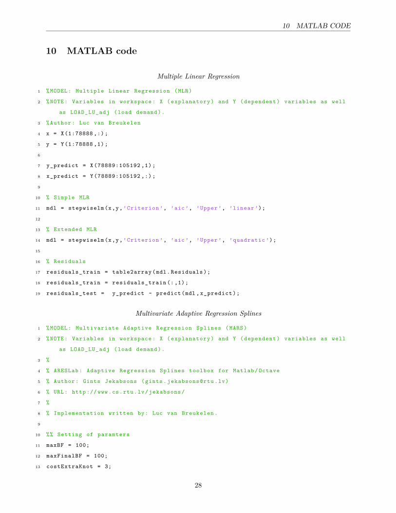
Multiple Linear Regression
1 %MODEL: Multiple Linear Regression (MLR)
2 %NOTE: Variables in workspace : X ( explanatory ) and Y ( dependent ) variables as well
as LOAD_LU_adj (load demand ).
3 % Author : Luc van Breukelen
4 x = X (1:78888 ,:) ;
5 y = Y (1:78888 ,1) ;
6
7 y_predict = X (78889:105192 ,1) ;
8 x_predict = Y (78889:105192 ,:) ;
9
10 % Simple MLR
11 mdl = stepwiselm (x,y,’Criterion ’, ’aic ’, ’Upper ’, ’linear ’);
12
13 % Extended MLR
14 mdl = stepwiselm (x,y,’Criterion ’, ’aic ’, ’Upper ’, ’quadratic ’);
15
16 % Residuals
17 residuals_train = table2array (mdl. Residuals );
18 residuals_train = residuals_train (: ,1);
19 residuals_test = y_predict - predict (mdl , x_predict );
Multivariate Adaptive Regression Splines
1 %MODEL: Multivariate Adaptive Regression Splines (MARS)
2 %NOTE: Variables in workspace : X ( explanatory ) and Y ( dependent ) variables as well
as LOAD_LU_adj (load demand ).
3 %
4 % ARESLab : Adaptive Regression Splines toolbox for Matlab / Octave
5 % Author : Gints Jekabsons (gints. jekabsons@rtu .lv)
6 % URL: http :// www.cs.rtu.lv/ jekabsons /
7 %
8 % Implementation written by: Luc van Breukelen .
9
10 %% Setting of paramters
11 maxBF = 100;
12 maxFinalBF = 100;
13 costExtraKnot = 3;
28

10 MATLAB CODE
14 maxInteraction = 3;
15 params = aresparams2 (’maxFuncs ’, maxBF , ’maxFinalFuncs ’, ...
16 maxFinalBF , ’c’, costExtraKnot , ’maxInteractions ’, maxInteraction ,...
17 ’cubic ’, false ); % piecewise - linear without minSpan
18
19 params = aresparams2 (’maxFuncs ’, maxBF , ’maxFinalFuncs ’, ...
20 maxFinalBF , ’c’, costExtraKnot , ’maxInteractions ’, maxInteraction ,...
21 ’cubic ’, false , ’useMinSpan ’, 500 ); % piecewise - linear with minSpan
22 %% Load data
23 y = Y (1:78888 ,1) ;
24 x = X (1:78888 ,:) ;
25
26 y_predict = X (78889:105192 ,1) ;
27 x_predict = Y (78889:105192 ,:) ;
28 %% Build model
29 disp(’Building the model ================================================== ’);
30 [model , ˜, resultsEval ] = aresbuild (x, y, params );
31 %% Plotting model selection from the backward pruning phase
32 figure ;
33 hold on; grid on; box on;
34 h(1) = plot( resultsEval .MSE , ’Color ’, [0 0.447 0.741]) ;
35 h(2) = plot( resultsEval .GCV , ’Color ’, [0.741 0 0.447]) ;
36 numBF = numel(model.coefs);
37 h(3) = plot ([ numBF numBF], get(gca , ’ylim ’), ’--k’);
38 xlabel (’Number of basis functions ’);
39 ylabel (’MSE , GCV ’);
40 legend (h, ’MSE ’, ’GCV ’, ’Selected model ’);
41 %% Info on the basis functions
42 disp(’Info on the basis functions ========================================= ’);
43 aresinfo (model , x, y);
44
45 % Printing the model
46 disp(’The model =========================================================== ’);
47
48 %% Testing on test data
49 disp(’Testing on test data ================================================ ’);
50 results = arestest (model , x_predict , y_predict );
51
52 % Residuals
29

10 MATLAB CODE
53 residuals_train = y- arespredict (model , x);
54 residuals_test = y_predict - arespredict (model , x_predict );
Artificial Neural Network
1 %MODEL: Artifical Neural Network (ANN)
2 %NOTE: Variables needed in workspace : X and Y ( explanatory & dependent variables )
as well as LOAD_LU_adj (load demand ).
3 % Author : Luc van Breukelen
4
5 % Data
6 y = Y (1:78888 ,1) ’;
7 x = X (1:78888 ,:) ’;
8
9 y_predict = X (78889:105192 ,1) ’;
10 x_predict = Y (78889:105192 ,:) ’;
11
12 % Create a Fitting Network
13 trainFcn = ’trainlm ’;
14 hiddenLayer1Size = 15;
15 hiddenLayer2Size = 15;
16 net = fitnet ([ hiddenLayer1Size , hiddenLayer2Size ], trainFcn );
17
18 % Set sigmoid functions
19 net. layers {1}. transferFcn = ’logsig ’;
20 net. layers {2}. transferFcn = ’logsig ’;
21 net. layers {3}. transferFcn = ’purelin ’;
22 net. performFcn = ’sse ’;
23
24 % Set up Division of Data for Training , Validation , Testing
25 net. divideParam . trainRatio = 75/100;
26 net. divideParam . valRatio = 25/100;
27 net. divideParam . testRatio = 0/100;
28
29 % Train network
30 [net ,tr] = train(net ,x,y);
31
32 % Residuals
33 residuals_train = y-net(x);
34 residuals_test = y_predict -net( x_predict );
30

10 MATLAB CODE
Double Seasonal Block Bootstrap
1 % Double seasonal block bootstrap method for 2015 , 2016 and 2017
2 %NOTE: Workspace need to consist the x matrix with explanatory variables .
3 % Author : Luc van Breukelen
4
5 number_of_scenarios = 1000;
6 weather_scenarios = cell( number_of_scenarios ,1);
7 number_variables = 7;
8 number_observations = 26304;
9 scenario = zeros( number_observations , number_variables );
10 default_length = 91*24;
11 year = 24*365;
12
13 for scenario_number = 1 : number_of_scenarios
14 % First year is no leap year.
15 for season = 1:4
16 [ start_index , end_index ] = getIndex (0, season );
17 scenario (1+( season -1)* default_length :(1+( season -1)* default_length )+(
end_index - start_index ) ,:) = x( start_index :end_index ,:);
18 end
19 % Second year is leap year
20 for season = 1:4
21 [ start_index , end_index ] = getIndex (1, season );
22 if season ==2
23 scenario (year +1+( season -1)* default_length :8761+( season -1)*
default_length +( end_index - start_index ) ,:) = x( start_index :end_index
,:);
24 elseif season >2
25 scenario (year +1+( season -1)* default_length +24: year +1+( season -1)*
default_length +24 +( end_index - start_index ) ,:) = x( start_index :
end_index ,:);
26 else
27 scenario (year +1+( season -1)* default_length :year +1+( season -1)*
default_length +( end_index - start_index ) ,:) = x( start_index :
end_index ,:);
28 end
29 end
30 % Third year is no leap year.
31 for season = 1:4
31

10 MATLAB CODE
32 [ start_index , end_index ] = getIndex (0, season );
33 scenario (year *2+24+( season -1)* default_length +1: year *2+24+( season -1)*
default_length +1+ (end_index - start_index ) ,:) = x( start_index :end_index
,:);
34 end
35 weather_scenarios { scenario_number } = scenario ; %Save scenario of 3 year.
36 end
Function for double seasonal block bootstrap
1 function [ start_index , end_index ] = getIndex (leap , season )
2 % GETINDEX Generate start and end indices of block.
3 % INPUT:
4 % leap Dummy variable which is 1 when year is a leap year
5 % season Integer between [1 ,4] which represents number of block.
6 % OUTPUT :
7 % start_index Start index of block.
8 % end_index End index of block.
9 % Author : Luc van Breukelen
10
11 length_block = 2184;
12 max_index = 78888;
13
14 if (leap ==1 && season == 2) || season == 4
15 length_block = length_block + 24; % Period with extra day (leap year).
16 end
17
18 i = 1 + floor(rand *9); % Randomly select a year from historical dataset .
19
20 % Uniformly integer in [ -14 ,14]
21 random = floor(rand * 24*28) -14*24;
22 random = random - mod(random ,24);
23
24 start_index = max (1+(i -1) *8760+( season -1) *2184+ random ,1);
25 end_index = start_index + length_block -1;
26 if end_index > max_index % Correction at end of data set.
27 end_index = max_index ;
28 start_index = max_index - length_block +1;
29 end
30 end
32