On the dynamics of commercial

�shing and parameter identi�cation

Al-Amin M. Ussif 1, Leif K. Sandal 2 and Stein I. Steinshamn 3

May 2000

Abstract

This paper has two main objectives. The �rst is to develop dynamic models of commercial

�sheries di�erent from the existing models. The industry is assumed to have a well

de�ned index of performance based on which it either invests or otherwise. We do not

however, assume that the industry or �rm is e�cient or optimal in its operations. The

hypotheses in the models are quite general, making the models applicable to di�erent

management regimes. The second is that a new approach of �tting model dynamics

to time series data is employed to simultaneously estimate the poorly known initial

conditions and the parameters of the nonlinear �sheries dynamics. The approach is a

data assimilation technique known as the adjoint method. Estimation of the poorly

known initial conditions is one of the attractive features of the adjoint method. Unlike

the conventional methods, the method employed in this paper, requires relatively less

data. Economic parameters were reasonably estimated without cost and price data. The

estimated equilibrium biomass is very close to the maximum sustainable biomass which

means open access in this case led to economic over�shing but not biological over�shing.

1Department of Finance and Management Science, Norwegian School of Economics and Business

Administration, Bergen Norway. Corresponding author: Tel. +4755959686, Fax . +4755959234,

Email:ussif@hamilton.nhh.no.2Norwegian School of Economics and Business Administration, Bergen Norway.3Foundation for Research in Economics and Business Administration, Bergen Norway.

1

Keywords: Data assimilation; adjoint method; index of performance; nonlinear dynamics;open access

JEL classi�cation:Q22,C51

2

1 Introduction

The most common approaches of modeling the dynamics of a natural resource system

are by the routine application of the sophisticated techniques of the calculus of varia-

tions or optimal control theory and dynamic programming (Kamien and Schwartz, 1984;

Clark, 1990). The economic theory of an optimally managed �shery has been advanced

by many researchers. Clark (1990) discussed various models in some detail. Sandal and

Steinshamn (1997a,b,c) made some of the most recent contributions in the area. These

frameworks explicitly assume that agents are optimal and e�cient. However, most real

world �sheries have historically not been optimally managed.

The dynamics of single species models have extensively been studied in the literature

of natural resource economics (Sandal and Steinshamn, op. cit.). Extensions have also

been made to include ecological e�ects from other species. The simplest is the predator-

prey model (see Clark, 1990).

Commercial models of �sheries have previously been discussed by Crutch�eld and Zell-

ner (1962) and Smith (1967). The latter provided a model of theoretical nature which

transforms speci�c patterns of assumptions about cost conditions, demand externalities

and biomass growth technology into a pattern of exploitation of the stock. Smith also

discussed the three main features of commercial �shing and mentioned the various types

of external e�ects representing external diseconomies to the industry. In two earlier

papers, Gordon (1954) and Scott (1955) noted that all of these externalities arise fun-

damentally because of the unappropriated \common property" character of most ocean

�sheries (Smith, 1967).

3

In this paper, we develop some commercial �shing models that do not necessarily assume

optimal behavior of �shers. The goal is to develop models that are quite general and

have much wider possible applications. Models of natural resource exploitation consist

of two vital components. First, a sound biological base which de�nes the environmental

and ecological constraints is required. Second, an economic submodel that incorporates

the basic characteristics of the exploiting �rms must be in place. For example, an in-

dustry or a �rm may be assumed to vary levels of capital investments in proportion to

some measurable quantities such as the total pro�ts (Smith, 1967; Clark, 1979).

This paper also focuses on a very important aspect of �sheries management that has

largely been ignored. Deacon et al. (1998) noted that much of the information managers

need is empirical, i.e., measurements of vital relationships and judgments about various

impacts. This area of the economics of �shing has not been adequately explored by

economists probably due to lack of data and computational power in the past. Much

of the research e�orts were used in the search for qualitative answers to management

problems.

This paper employs a new and e�cient method of advanced data assimilation known as

the adjoint technique (Smedstad and O'Brien, 1991) to analyze real �sheries data. In

data assimilation, mathematical or numerical models are merged with observational data

in order to improve the model itself or to improve the model predictions. The former

application is known as model �tting. Using the adjoint technique, in which the model

dynamics are often assumed to be perfect, i.e., the dynamical constraints are satis�ed

exactly (Sasaki, 1970), appropriate initial conditions and parameters of the nonlinear

�sheries dynamics are estimated. Nonlinear �sheries dynamics are highly sensitive to

4

the initial conditions and the parameters which are often exogenously given inputs to

the system. These inputs are very crucial in simulation studies. Inverse methods and

data assimilation are often ill-posed, i.e., they are characterized by nonuniqueness and

instability of the identi�ed parameters (Yeh, 1986). It may thus be worthwhile to search

for best initial and/or boundary conditions when using these models in analysis. The

reader may have noticed that this approach has major advantages compared to conven-

tional methods. It allows us to estimate initial conditions of the model dynamics as

additional control variables on equal footing as the model parameters. Thus, treating

the initial biomass level and the initial harvest rate as uncertain inputs in the system.

Most recent models and traditional approaches consider the initial biomass and harvest

amounts as known and deterministic. It also provides an e�cient way of calculating

the gradients of the loss function with respect to the control variables. Most impor-

tantly, data requirements are signi�cantly reduced. In this paper, parameters entering

the objective function of the industry have been reasonably estimated without having

to use data on prices and costs. Large number of parameters could be estimated with

observations on only a subset of the variables.

The structure of the remainder of the paper is as follows. Section 2 is a detailed dis-

cussion of the dynamics of the commercial �shing model. It presents a more general

model without assuming any optimizing behavior. In section 3, we brie y discuss data

assimilation and some basic concepts of the techniques are de�ned. All technical details

are put in an Appendix. Section 4 is an application to the Norwegian cod �shery (NCF).

It discusses the results and summarizes the work.

5

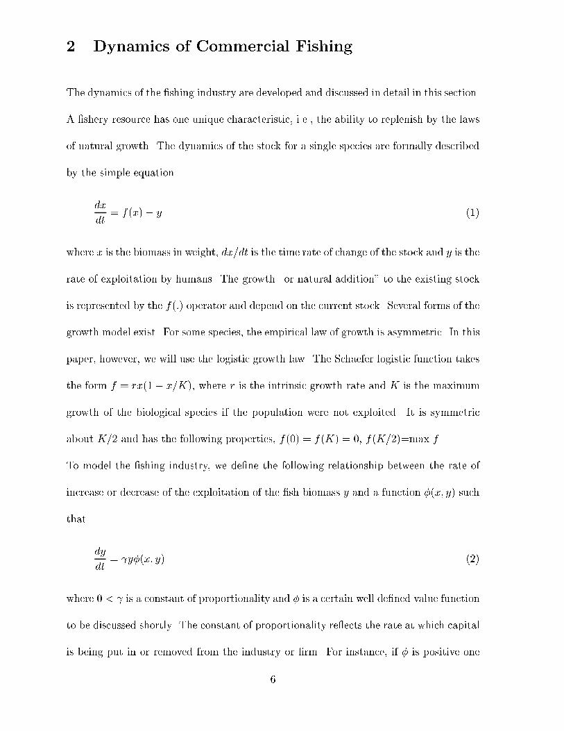
2 Dynamics of Commercial Fishing

The dynamics of the �shing industry are developed and discussed in detail in this section.

A �shery resource has one unique characteristic, i.e., the ability to replenish by the laws

of natural growth. The dynamics of the stock for a single species are formally described

by the simple equation

dx

dt= f(x)� y (1)

where x is the biomass in weight, dx=dt is the time rate of change of the stock and y is the

rate of exploitation by humans. The growth \or natural addition" to the existing stock

is represented by the f(:) operator and depend on the current stock. Several forms of the

growth model exist. For some species, the empirical law of growth is asymmetric. In this

paper, however, we will use the logistic growth law. The Schaefer logistic function takes

the form f = rx(1� x=K), where r is the intrinsic growth rate and K is the maximum

growth of the biological species if the population were not exploited. It is symmetric

about K=2 and has the following properties, f(0) = f(K) = 0, f(K=2)=max f .

To model the �shing industry, we de�ne the following relationship between the rate of

increase or decrease of the exploitation of the �sh biomass y and a function �(x; y) such

that

dy

dt= y�(x; y) (2)

where 0 < is a constant of proportionality and � is a certain well de�ned value function

to be discussed shortly. The constant of proportionality re ects the rate at which capital

is being put in or removed from the industry or �rm. For instance, if � is positive one

6

may expect an increase in capital investment in the �shery and a decrease otherwise. The

function(s) de�ned by � can take di�erent parametric forms re ecting our hypotheses

about the operation of the industry. It may represent short or long run average costs of

�shing vessels, the marginal or average net revenues of a �rm, etc. Di�erent forms of the

� functions will be discussed in detail. We will �rst model an industry that is perceived

to be a price taker in the output market.

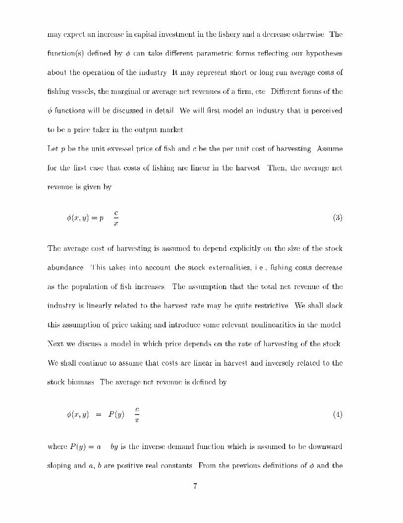
Let p be the unit exvessel price of �sh and c be the per unit cost of harvesting. Assume

for the �rst case that costs of �shing are linear in the harvest. Then, the average net

revenue is given by

�(x; y) = p�c

x(3)

The average cost of harvesting is assumed to depend explicitly on the size of the stock

abundance. This takes into account the stock externalities, i.e., �shing costs decrease

as the population of �sh increases. The assumption that the total net revenue of the

industry is linearly related to the harvest rate may be quite restrictive. We shall slack

this assumption of price taking and introduce some relevant nonlinearities in the model.

Next we discuss a model in which price depends on the rate of harvesting of the stock.

We shall continue to assume that costs are linear in harvest and inversely related to the

stock biomass. The average net revenue is de�ned by

�(x; y) = P (y)�c

x(4)

where P (y) = a � by is the inverse demand function which is assumed to be downward

sloping and a, b are positive real constants. From the previous de�nitions of � and the

7

industry model, equation (2), it is obvious that the rate of harvesting from the stock for

the industry is perceived to vary in proportion to the net revenue; that is the di�erence

between total revenues and total costs. Put another way, the output growth rate _y=y of

the industry is proportional to the average or marginal net revenues.

Substituting these functions in equation (2) and combining with the population dynamics

model, equation (1), the industry dynamics models are derived. This system of equations

(1)-(2) constitute coupled nonlinear ODEs. For the empirical analysis, we will use the

following models.

model 1

dx

dt= f(x; r;K)� y

dy

dt= (p�

c

x)y (5)

In the �rst model, the term (py � cy=x) is the annual total pro�t (total revenues minus

total costs). Owing to the linearity of the net revenue in the harvest, the average net

revenue is equal to the marginal net revenue.

model 2

dx

dt= f(x; r;K)� y (6)

dy

dt= (P (y)�

c

x)y

In model 2, the demand function is downward sloping, i.e., the output of the industry

a�ects its market price and costs are linear in harvest and inversely related to the stock

biomass (Sandal and Steinshamn, 1997b). Hence, the pro�t function is nonlinear both

8

in the harvest and the biomass. Incorporated in these models are the hypotheses about

the costs and the revenues. If the �rms were optimizers, they should at least operate

at a level where average or marginal pro�ts are positive. In the construction of such

behavioral models, an implicit assumption about the harvest rate being proportinal to

the number of �rms or �shing vessels is made (see simth 1967).

The system of equations contains these input parameters, the biological parameters

(r;K) and the economic parameters ( ; p; a; b; c). It is possible to estimate all of the

parameters in the models but additional data may be required. To obviate the data

problem, we reduce the dimension of the problem by rede�ning the parameters: � = p,

� = a, � = b, and � = c. That is, we now have these parameters (r;K; �; �; �; �)

to estimate. Notice here that no data on prices and costs are necessary in order to �t

the models. The method enables us to �t the bioeconomic models without using data

on economic variables which are often unavailable. These mathematical models of the

commercial �shing will be used to analyze real �shery data for the Norwegian cod �shery

(NCF) stock.

3 Data Assimilation Methods

Data assimilation methods have been used extensively in meteorology and oceanography

to estimate the variables of model dynamics and/or the initial and boundary conditions.

These methods include the sequential techniques of Kalman �ltering (Kalman, 1960) and

the variational inverse approach (Bennett, 1992). The variational adjoint method has

been proposed as a tool for estimation of model parameters. It has since proven to be

9

a powerful tool for �tting dynamic models to data (Smedstad and O'Brien, 1991). The

methods have recently been used to estimate parameters of the predator-prey equation

(Lawson et al., 1995) and also some high dimensional ecosystem models (Spitz et al.,

1997 and Matear, 1995). The basic idea is that, given a numerical model and a set of

observations, a solution of the model that is as close as possible to the observations is

sought by adjusting model parameters such as the initial conditions. The adjoint method

has three parts: the forward model and the data which are used to de�ne the penalty

function, the backward model derived via the Lagrange multipliers and an optimization

procedure. These components and all of the mathematical derivations are discussed in an

Appendix. An outline of the technique is also presented for those who may be interested

in learning the new and e�cient method of data analysis.

4 An Application

The commercial �shing models developed in this paper are used in an application to

NCF stock. The �shery has a long history of supporting large part of the Norwegian and

Russian coastal populations. Data on catches and estimated stock biomass have been

collected since immediately after World War II. Di�erent techniques of stock assessments

exist in �sheries management. The data on the NCF are measured using the statistical

Virtual Population Analysis (VPA) method. Catch data and biomass estimates obtained

by the VPA may be somewhat correlated. This issue will not be dealt with in this pa-

per.

The history of this �shery is not dissimilar from other commercial �sheries elsewhere

10

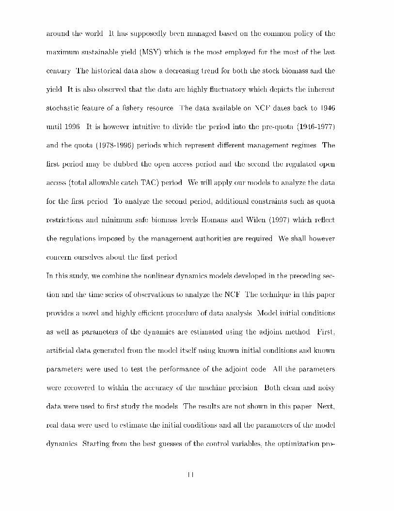
around the world. It has supposedly been managed based on the common policy of the

maximum sustainable yield (MSY) which is the most employed for the most of the last

century. The historical data show a decreasing trend for both the stock biomass and the

yield. It is also observed that the data are highly uctuatory which depicts the inherent

stochastic feature of a �shery resource. The data available on NCF dates back to 1946

until 1996. It is however intuitive to divide the period into the pre-quota (1946-1977)

and the quota (1978-1996) periods which represent di�erent management regimes. The

�rst period may be dubbed the open access period and the second the regulated open

access (total allowable catch TAC) period. We will apply our models to analyze the data

for the �rst period. To analyze the second period, additional constraints such as quota

restrictions and minimum safe biomass levels Homans and Wilen (1997) which re ect

the regulations imposed by the management authorities are required. We shall however

concern ourselves about the �rst period.

In this study, we combine the nonlinear dynamics models developed in the preceding sec-

tion and the time series of observations to analyze the NCF. The technique in this paper

provides a novel and highly e�cient procedure of data analysis. Model initial conditions

as well as parameters of the dynamics are estimated using the adjoint method. First,

arti�cial data generated from the model itself using known initial conditions and known

parameters were used to test the performance of the adjoint code. All the parameters

were recovered to within the accuracy of the machine precision. Both clean and noisy

data were used to �rst study the models. The results are not shown in this paper. Next,

real data were used to estimate the initial conditions and all the parameters of the model

dynamics. Starting from the best guesses of the control variables, the optimization pro-

11

cedure uses the gradient information to �nd optimal initial conditions and parameters

of the model which minimize the penalty function. The procedure is e�cient and �nds

the optimum solution in a matter of a few seconds. The estimated initial conditions and

parameters of the two di�erent models are tabulated below.

Parameters Model 1 Model 2

r 0.3271 0.44305

K 5264.85 5257.55

� 0.13039

� 4.1368

� .00213

� 309.01 7070.63

x0 3902.77 3670.00

y0 716.15 770.33

Table 1: Model parameters for the two dynamic models. Blank space means the param-

eter is not present in that model.

All the estimated parameters are reasonable and as expected. From the table above, the

estimated r's are di�erent for the two di�erent models. Model 2 which is more complex

than model 1 gives a bigger r value. The maximum population K is about the same

for both models. The initial conditions have also been adjusted in both cases. Note

that the observed initial values were taken as the best guesses. To further explain the

performance of these models, we present some graphics of the time series of the actual

12

observations and the estimated quantities. Figure 1 is a plot of the actual observations

(Act. observations) and the models predictions (Est. model 1 and Est. model 2) of the

stock biomass using the estimated parameters.

1945 1950 1955 1960 1965 1970 1975 19801500

2000

2500

3000

3500

4000

4500

Time(yrs)

Sto

ck b

iom

ass

(103 to

ns)

Act. observationsEst. model 1 Est. model 2

Figure 1: Graphs of the actual and the model estimated stock biomass for the two

models

It is observed that, model 1 predicts higher biomass levels and is generally steeper than

model 2. The models have both performed well in tracking the downward trend in the

data. Model 2 seems to do a little bit better overall and at the tail end of the data. In

Figure 2, we have the plot of the actual observations (Act. observations) and the model

predictions (Est. model 1 and Est. model 2) of the rate of harvesting.

13

1945 1950 1955 1960 1965 1970 1975 1980400

500

600

700

800

900

1000

1100

1200

1300

1400

Har

vest

(10

3 tons

)

Time(yrs)

Act. observationsEst. model 1 Est. model 2

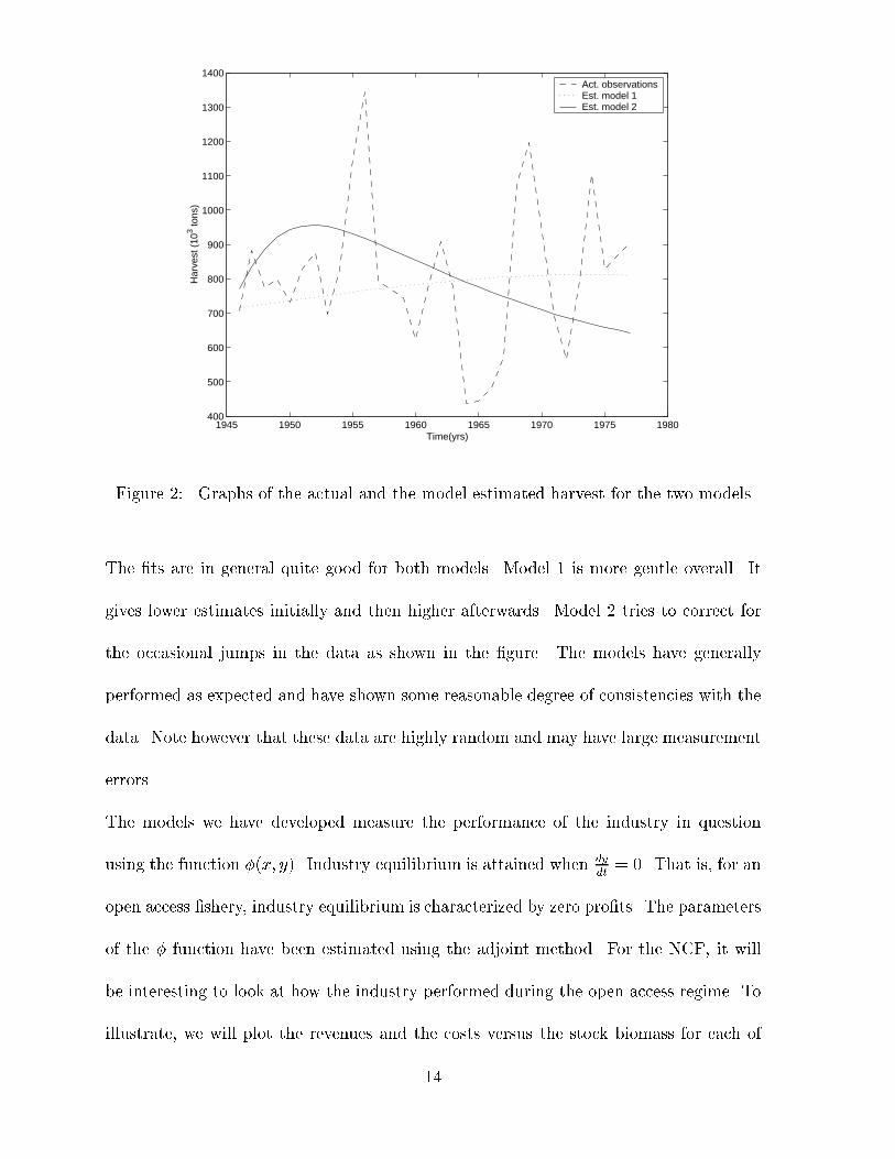
Figure 2: Graphs of the actual and the model estimated harvest for the two models

The �ts are in general quite good for both models. Model 1 is more gentle overall. It

gives lower estimates initially and then higher afterwards. Model 2 tries to correct for

the occasional jumps in the data as shown in the �gure. The models have generally

performed as expected and have shown some reasonable degree of consistencies with the

data. Note however that these data are highly random and may have large measurement

errors.

The models we have developed measure the performance of the industry in question

using the function �(x; y). Industry equilibrium is attained when dy

dt= 0. That is, for an

open access �shery, industry equilibrium is characterized by zero pro�ts. The parameters

of the � function have been estimated using the adjoint method. For the NCF, it will

be interesting to look at how the industry performed during the open access regime. To

illustrate, we will plot the revenues and the costs versus the stock biomass for each of

14

the two models. The revenue and cost functions are scaled by the parameter and the

unit of currency is the Norwegian Kroner (NOK).

In �gure 3 the total revenues and total costs are graphed. The di�erence between these

represent the net pro�ts. Costs were least when the stock size was largest but increased

as the stock decreased. The pro�ts were driven to zero when x� = c=p, i.e., the industry

is in a steady state. The industry equilibrium (point where total costs balance total

revenues) was reached at the stock level of x� = 2370 103tons which is the so called open

access equilibrium. This is lower but very close to the xMSY=(K=2) level. A further

reduction of the stock led to unpro�table investments. Costs exceeded revenues as the

stock level fell beyond x� = c=p.

2000 2200 2400 2600 2800 3000 3200 3400 3600 3800 400050

60

70

80

90

100

110

120

Am

ount

(10

3 NO

K)

Stock biomass (103tons)

Tot. revenuesTot. costs

Figure 3: Graphs of the total revenues and the total costs vs. estimated stock biomass

for model 1.

Figure 4 is a plot of the revenue and cost functions. The shapes of the functions indicate

15

their level of complexities. The results of model 2 have some similar characteristics to

model 1. However, the industry steady state occurred at a higher biomass level of about

3400 Kilo-tons. Extrapolation of the results of model 2 indicate another equilibrium

x� = 2440 103tons close to the one predicted by model 1. This point satis�es the

equilibrium conditions _x = _y = 0. The hypothesis of a large industry whose output

a�ects the market price resulted in a multiple industry equilibria. The �rst is quite

unstable since only the industry reached equilibrium but not the biology. The biological

and industry steady state occurred at the second point (extrapolation not shown).

2400 2600 2800 3000 3200 3400 3600 38001400

1500

1600

1700

1800

1900

2000

2100

Stock biomass (103tons)

Am

ount

(10

3 NO

K)

Tot. revenuesTot. costs

Figure 4: Graphs of the total revenues and the total costs vs. estimated stock biomass

for model 2.

In both models, costs are assumed to be inversely related to the stock biomass. This

underscores stock externalities in the models which appear to reasonably characterize

the NCF. Note that the cod is a demersal species and does not exhibit the schooling

16

characteristics of the species such as herring. Both models will attain bioeconomic steady

state at about the same biomass level of little below the MSY biomass level. The question

of which of these models is more appropriate for the NCF is still immature to give a

de�nite answer to. More research needs to be done. What is certain is that with

more realistic models and data with less errors than the one available, it is possible to

operationalize modern �sheries management.

4.1 Summary and conclusion

This paper, unlike most other papers, has addressed two major questions in bioeconomic

analysis and �sheries management. It developed simple dynamic �sheries models in a

way that is rare in the literature and employs a new and powerful approach of e�ciently

combining these models with available observations collected over a given time domain.

The adjoint method is used to simultaneously estimate the initial conditions and the

input parameters of the industry �shing models. An interesting �nding of the paper,

is that, the steady state without regulation is not too far away from the MSY. Which

means that, open access in this case has meant economic over�shing but not necessarily

biological over�shing. It is observed that the technique used in this paper has an added

virtue compared to the conventional ones used in the literature. Initial conditions of the

model dynamics are estimated on equal footing as the model parameters. It is highly

versatile that, it enables researchers to include as much information as is available to

them. The estimates were all reasonable and as expected for the NCF. The models

have quite reasonable explanatory power. However caution must be exercised when

interpreting the results due to the inadequacy of the models and the large measurement

17

errors in the data.

It has been demonstrated here that, dynamic resource models can be combined with real

data in order to obtain useful insights about real �sheries. Biological parameters such as

the carrying capacity and economic parameters entering the objective functions of the

industry are identi�ed. These again can be used for dynamic optimization in order to

improve the economic performance of the �shery. The adjoint method has proven to be

very promising and deserves further research e�orts not only in resource economics but

economics in general.

APPENDIX A

A.1 Data Assimilation-A Background

This section formulates the parameter estimation problem and presents the mathematical

aspects of the adjoint technique. Numerical issues have also been brie y discussed.

A.1.1 The model and the data

The model dynamics are assumed to hold exactly, i.e., the dynamics are perfect. The

dynamics are described by the two models above. For the sake of mathematical conve-

nience, we use the compact notation to represent the model dynamics as

dX

dt= F (X;Q) (A.1)

X(0) = X0 + X̂0 (A.2)

18

Q = Q0 + Q̂ (A.3)

where X = (x; y) is the state vector, X0 is the best guess initial condition vector, X̂0 is

the vector of initial mis�ts, Q is a vector of parameters and Q̂ is the vector of parameter

mis�ts. The dynamics are assumed to exactly satisfy the constraints while the inputs,

i.e., the initial conditions and the parameters are poorly known.

In real world situations, observations are often available for some variables such as the

annual catches and �shing e�orts. The set of observations are often sparse and noisy

and are related to the model counterparts in some fashion. The measurement vector is

de�ned by

X̂ = H[X] + � (A.4)

where X̂ is the measurement vector, � is the observation error vector and H is a lin-

ear measurement operator. The mis�ts are assumed to be independent and identically

distributed \iid" random deviates. To describe the errors in the initial conditions, the

parameters and the data, we require some statistical hypotheses. For our purpose in this

paper the following hypotheses will su�ce

�̂X0 = 0; X̂0X̂

T0 =W�1

X0

�� = 0; ��T =W�1

�̂Q = 0; Q̂Q̂T = W�1

Q

where the T denotes matrix transpose operator. That is, we are assuming that the errors

are normally distributed with zero means and constant variances (homoscedastic) which

19

are ideally the inverses of the optimal weights. For this paper, it will further be assumed

that the errors are not serially correlated. This implies that the covariance matrices are

now diagonal matrices with the variances along the diagonal. We further assume that

the variances are constant.

A.1.2 The loss or penalty function

In adjoint parameter estimation, a loss functional which measures the di�erence between

the data and the model equivalent of the data is minimized by tuning the control variables

of the dynamical system. The goal is to �nd the parameters of the model that lead to

model predictions that are as close as possible to the data. A typical penalty functional

takes the more general form

J [X;Q] =1

2Tf

Z Tf

0

(Q�Q0)TWQ(Q�Q0)dt

+1

2Tf

Z Tf

0

(X(0)�X0)TW(X(0)�X0)dt

+1

2

Z Tf

0

(X� X̂)TW(X� X̂)dt (A.5)

where the period of assimilation is denoted by Tf and T is the matrix transpose operator.

The W0s are the weight matrices which are optimally the inverses of the error covari-

ances of the observations. They are assumed to be positive de�nite and symmetric. The

�rst and second terms in the penalty functional represent our prior knowledge of the

parameters and the initial conditions, and ensure that the estimated values are not too

far away from the �rst guesses. They may also enhance the curvature of the loss func-

tion by contributing positive terms to the Hessian of J (Smedstad and O'Brien, 1991).

20

The adjoint technique determines an optimal solution by minimizing the loss function

J which measures the discrepancy between the model predictions and the observations.

The loss function is minimized subject to the dynamics. The constrained inverse problem

above is e�ciently solved by transforming the problem into an unconstrained optimiza-

tion (Luenberger, 1984). Several algorithms for solving the unconstrained nonlinear

programming problem are available (Smedstad and O'Brien, 1991). Statistical methods

such as the simulated annealing (Matear, 1995; Kruger, 1992) and the Markov Chain

Monte Carlo (MCMC) (Harmon and Challenor, 1997) have recently been proposed as

tools for parameter estimation. The most widely used methods are the classical iterative

methods such as the gradient descent and the Newton's methods (see Luenberger, 1984).

A.1.3 The adjoint method

Construction of the adjoint code is identi�ed as the most di�cult aspect of the data

assimilation technique (Spitz et al., 1997). One approach consists of deriving the con-

tinuous adjoint equation and then discretizing them (Smedstad and O'Brien, 1991).

Another approach is to derive the adjoint code directly from the model code (Lawson et

al., 1995; Spitz et al., 1997). To illustrate the mathematical derivation, we use the �rst

approach (see details in Appendix). Formulating the Lagrange function L by appending

the model dynamics as strong constraints, we have

L[X;Q] = J +1

2

Z Tf

0

MdF

dXdt (A.6)

21

whereM is a vector of Lagrange multipliers which are computed in determining the best

�t. The original constrained problem is thus reformulated as an unconstrained problem.

At the unconstrained minimum the �rst order conditions are

dL

dX= 0 (A.7)

dL

dM= 0 (A.8)

dL

dQ= 0: (A.9)

It is observed that equation (A.7) results in the adjoint or backward model, equation

(A.8) recovers the model equations while (A.9) gives the gradients with respect to the

control variables. Using calculus of variations or optimal control theory, the adjoint

equation is derived by forming the Lagrange functional via the undetermined multipliers

M(t). The Lagrange function is

L = J +Z Tf

0

M(@X

@t� F (X;Q))dt (A.10)

Perturbing the function L

L[X+ �X;Q] = J [X+ �X;Q]

+1

2

Z Tf

0

M(@(X + �X)

@t� F (X+ �X;Q))dt

which implies

L[X+ �X;Q] = J +�XJ �XT +Z Tf

0

M(@X

@t� F (X;Q))dt

� 2Z Tf

0

M(@�X

@t�

@F

@X�XT )dt+O(�X2) (A.11)

22

Taking the di�erence (L[X+ �X;Q]� L[X;Q])

�L = �XJ �XT

� 2Z Tf

0

M(@�X

@t�

@F

@X�XT )dt+O(�X2) (A.12)

Requiring that �L be of order O(�X2) implies

�XJ �XT�

Z Tf

0

M(@�X

@t�

@F

@X�XT )dt = 0 (A.13)

By integrating the second term of the LHS by parts and rearranging, we have

@M

@t+ [

@F

@X]TM =W(X� X̂)

M(Tf) = 0 (A.14)

which is the adjoint equation together with the boundary conditions and from (A.8) the

gradient relation is

�QJ = �

Z Tf

0

MdF

dQdt+WQ(Q�Q0) (A.15)

The term on the RHS of (A.14) is the weighted mis�t which acts as forcing term for the

adjoint equation. It is worth noting here that we have implicitly assumed that data is

continuously available throughout the integration interval. Equations (A.7) and (A.8)

above constitute the Euler-Lagrange (E-L) system and form a two-point boundary value

problem. The implementation of the adjoint technique on a computer is straightforward.

The algorithm is outlined below.

� Choose the �rst guess for the control parameters.

23

� Integrate the forward model over the assimilation interval.

� Calculate the mis�ts and hence the loss function.

� Integrate the adjoint equation backward in time forced by the data mis�ts.

� Calculate the gradient of L with respect to the control variables.

� Use the gradient in a descent algorithm to �nd an improved estimate of the control

parameters which make the loss function move towards a minimum.

� Check if the solution is found based on a certain criterion.

� If the criterion is not met repeat the procedure until a satisfactory solution is found.

The optimization step is performed using standard optimization procedures. In this pa-

per, a limited memory quasi-Newton procedure (Gilbert and Lemarechal, 1991) is used.

The success of the optimization depends crucially on the accuracy of the computed gra-

dients. Any errors introduced while calculating the gradients can be detrimental and

the results misleading. To avoid this incidence from occurring, it is always advisable to

verify the correctness of the gradients (see, Smedstad and O'Brien, 1991; Spitz et al.,

1997).

Acknowledgements: Al-Amin Ussif wants to thank Dr. J.J. O'Brien of Center for

Ocean Atmospheric-prediction studies at FSU Tallahassee, Florida for letting me visit

his research center. I also wish to thank the following Dr. Hannesson, Dr Steve Morey

and Kim Lebby for reading my work and Gilbert and Lemarechal of INRIA in France for

24

letting me use their optimization routine. Financial support from the Norwegian School

of Economics and Business Administration is appreciated.

25

References

� Bennett, A.F., 1992, Inverse Methods in Physical Oceanography. (Cambridge Uni-

versity Press, Cambridge).

� Clark, W., 1979, Mathematical Models in the Economics of Renewable Resources,

SIAM Review,vol,21(1), 81-99.

� Clark, W., 1990. Mathematical Bioeconomics (New York: Wiley and Sons).

� Crutch�eld, J.A. and A. Zellner, 1962, Economic Aspects of the Paci�c Halibut

Fishery. Fishery Industrial Research. vol. 1(1). Washington: U.S. Department of

the Interior.

� Deacon, R.T., Brookshire, D.S, Fisher, A.C, Kneese, A.V., Kolstad, C.D.,Scrogin,

D., Smith, V.K., Ward, M. and J. Wilen, 1998, Research Trends and Opportunities

in Environmental and Natural Resource Economics. Journal of Environmental

Economics and Management, 11(3-4): 383-397.

� Gilbert, J. C. and C. Lemarechal, 1991. Some Numerical Experiments with Variable-

storage Quasi-newton Algorithms. Mathematical programming 45, 405-435.

� Gordon, H. S, 1954, The Economic Theory of Common Property Resources. Jour-

nal of Political Economy, LXII, No.2,124-142.

� Harmon, R. and P. Challenor, 1997. Markov Chain Monte Carlo Method for

Estimation and Assimilation into Models, Ecological Modeling, 101, 41-59.

� Homans, F. and J. Wilen, 1997, A Model of Regulated Open Access Resource Use.

Journal of Environmental Economics and Management, 32(1),1-21.

26

� Kalman, R. E., 1960, A New Approach to Linear Filter and Prediction Problem,

Journal of Basic Engineering, 82, 35-45.

� Lawson, L. M., Spitz, H. Y., Hofmann, E. E. and R. B. Long, 1995. A Data

Assimilation Technique Applied to Predator-Prey Model, Bulletin of Mathematical

Biology, 57, 593-617.

� Sandal, L. K. and S. I. Steinshamn, 1997a, A Stochastic Feedback Model for the

Optimal Management of Renewable Resources, Natural Resource Modeling, vol.

10(1), 31-52.

� Sandal, L. K. and S. I. Steinshamn, 1997b. A Feedback Model for the Optimal

Management of Renewable Natural Capital Stocks, Canadian Journal of Fisheries

and Aquatic Sciences, 54, 2475-2482.

� Sandal, L. K. and S. I. Steinshamn, 1997c. Optimal Steady States and E�ects of

Discounting. Marine Resource Economics, vol.,12, 95-105.

� Schaefer, M. B., 1967, Fisheries Dynamics and the Present Status of the Yellow

Fin Tuna Population of the Eastern Paci�c Ocean, Bulletin of the Inter-American

Tropical Tuna commission 1, 25-56.

� Scott, A., 1955, The Fishery: The Objectives of Sole Ownership, Journal of Polit-

ical Economy. LXIII, No.2, 116-124.

� Smedstad, O. M., and J. J. O'Brien, 1991. Variational Data Assimilation and Pa-

rameter Estimation in an Equatorial Paci�c Ocean Model, Progress in Oceanogra-

phy 26(10), 179-241.

27

� Smith, V. L, 1967. On Models of Commercial Fishing. Journal of Political Econ-

omy, 77, 181-198.

� Spitz, H. Y., Moisan, J. R., Abbott, M. R. and J. G. Richman, 1998. Data As-

similation and a Pelagic Ecosystem Model: Parameterization Using Time Series

Observations, Journal of Marine Systems, in press.

� Yeh, W. W-G., 1986, Review of Parameter Identi�cation Procedures in Ground-

water Hydrology: The Inverse Problem. Water Resource Research, 22, 95-108.

28