ba-02 giww/clovelly

Louisiana Department of Natural Resources Coastal

Restoration Division

Hydrodynamic and Salinity Modeling of BA-02

GIWW/CLOVELLY Hydrologic Restoration Project

May 10, 2006

135 Regency Square Lafayette, La. 70508 337.237.2200 www.fenstermaker.com

Engineers Surveyors Environmental Consultants

BA-02

GIWW/CLOVELLY

http://www.fenstermaker.com

C.H. Fenstermaker & Associates, Inc.

Lafayette Houston New Orleans Baton Rouge

TABLE OF CONTENTS

Description Page

Chapter 1 1.1 Project Background 1

1.2 Project Objective 2

1.3 Project Description 3

1.4 Adaptive Environmental Assessment and Management 5

Chapter 2 2.1 Model Selection 8

2.2 Data Collection & Review 9 2.2.1 Bathymetric Data 9 2.2.2 Hydrologic Data Collection 13

2.3 Model Setup 16 2.3.1 Setup of Channel Network 16 2.3.2 Model Boundary Conditions 17 2.3.3 Modeling of Hydraulic Structures 17

2.4 Model Calibration 18

2.5 Model Validation & Evaluation of Model Performance 21

2.6 Discussion of Limitation & Capabilities of the model 22

Chapter 3 3.1 Analysis of Model Results 29

3.4 Final conclusions and closing remarks 30



TABLE OF CONTENTS

(Continued)

Report Authors:

Ehab A. Meselhe PhD. P.E. Senior Hydraulic Engineer

Emad Habib PhD. Hydraulic Modeler

Karim Kheiashy MS., E.I. Hydraulic Modeler

i C.H. Fenstermaker & Associates, Inc.

Lafayette Baton Rouge New Orleans Houston

EXECUTIVE SUMMARY

The GIWW/Clovelly Hydrologic Restoration Project consists of 14,948 acres located in the Barataria Basin near the Gulf Intercoastal Waterway (GIWW) in Lafourche Parish, Louisiana. The project is bounded by the Gulf Intercoastal Waterway to the north and to the northeast, Bayou Lafourch to the west, Superior Canal to the south, Bayou Perot, Little Lake and Bayou L Ours to the east

LDNR has proposed using hydrodynamic and salinity numerical model to address two main goals set forth by the agency. These goals include the ability to evaluate the constructed project features and determine if the project has met the intended objectives of reducing the salinity and tidal exchange.

Based on the numerical model results, LDNR will be able to assess whether or not the constructed project features will remain as they are or need design modification.

The use of a numerical model for this project has provided a tool for the assessment of the effectiveness of each of the constructed project structures. The model was calibrated and validated against field measurements. The model provided information regarding salinity and water level fluctuations, velocities, and discharges within the project area and near the existing structures. The salinity transport was computed through an Advection Dispersion (AD) module, coupled with the hydrodynamic module.

The model results illustrated that having all the structures in place reduced salinity in the southern project area (in the magnitude of 3-4 ppt on average at gauge 55 and 58). Structure 14A by itself appears to have only a local effect in the Clovelly Canal around the structure itself. Having the structure in place reduced the salinity in the Clovelly canal (4 -5 ppt at gauge 54).

Reducing the size of the weir opening provided additional salinity reduction (an additional 2-3 ppt at gauge 54), however this salinity reduction was not noticed on the southern portion of the project (gauge 55 and 58). This salinity reduction was noticed on the hourly scale and also the monthly scale.



1

PROJECT BOUNDARY

Mississippi River

Lake Ponchetrain

Lake Salvador

Gulf of Mexico

Lake Borgne

N

I. CHAPTER ONE

1.1 PROJECT BACKGROUND

The GIWW/Clovelly Hydrologic Restoration Project consists of 14,948 acres located in the Barataria Basin near the Gulf Intercoastal Waterway (GIWW) in Lafourche Parish, Louisiana. The project is bounded by the Gulf Intercoastal Waterway to the north and to the northeast, Bayou Lafourch to the west, Superior Canal to the south, Bayou Perot, Little Lake and Bayou L Ours to the east as shown in Figures 1.1 & 1.2.

Construction of the GIWW to Clovelly Restoration Project was authorized by Section 303(a) of Title III Public Law 101-646, the Coastal Wetlands Planning, Protection and Restoration Act (CWPPRA) enacted on November 29, 1990 as amended. The GIWW to Clovelly Project was approved on the first Priority Project List1.

Figure 1.1: Project Location Map

1 2004 Annual Inspection Report for GIWW/CLOVELLY Hydrologic Restoration, State Project Number BA-02, Priority Project List 1. Prepared by Brian. Babin, P.E. LDNR/Coastal Restoration and Management



2

Gulf of Mexico

Lake Salvador

GIWW

Bayou Lafourche

Mississippi River

Little Lake

Bayou Rigollete

Bayou Perot

PROJECT BOUNDARY

Bayou L Ours

Figure 1.2: Project Boundary showing major water bodies in the surrounding area

1.2 PROJECT OBJECTIVE

LDNR has proposed using hydrodynamic and salinity numerical model to address two main goals set forth by the agency. These goals include the ability to:

Evaluate the constructed project features.

Identify any deficiencies and recommend any corrective actions if necessary

Based on the numerical model results, LDNR will be able to assess whether or not the constructed project features will remain as they are or need design modification

The use of a numerical model for this project has provided a tool for the assessment of the effectiveness of each of the constructed project structures. The model was calibrated and validated against field measurements. The model provided information regarding salinity and water level fluctuations, velocities, and discharges within the project area and near the existing structures. The salinity transport was computed through an Advection Dispersion (AD) module, coupled with the hydrodynamic module. The final results for water level, and salinity were displayed though time series graphical plots, animated time series illustrations.

N



3

1.3 PROJECT DESCRIPTION

Within the GIWW to Clovelly Hydrologic Restoration Project, the average rate of change from marsh habitat to non-marsh habitat (including wetland loss to both open water and commercial development) has been increasing since the 1950s. The main reasons for wetland deterioration in the project area as reported by the Natural Recourses Conservation Services (NRCS) in the Wetland Value Assessment (WVA) are saltwater instruction, oil field activities, subsidence, lack of sedimentation, and reduced freshwater influx. The construction of oilfield canals has also helped to produce negative impacts on coastal marshes of Louisiana

The purpose of the GIWW/Clovelly Project is to protect intermediate march in the project area by restoring natural hydrologic conditions that promote greater use of available freshwater and nutrients. This will be accomplished by limiting rapid water level changes, slowing water exchange through over-bank flow, reducing rapid salinities increases, and reducing saltwater intrusions (LDNR monitoring Plan, 1997). The project objectives and goals as outlined in the Monitoring Plan drafted by LDNR are the following:

Project Objectives are as follows:

Protect and maintain approximately 14,948 acres of intermediate marsh by restoring natural hydrologic conditions that promote greater freshwater retention and utilization, prevent rapid salinity increases, and reduce the rate of tidal exchange

Reduce shoreline erosion through shoreline stabilization

The goals are as follows:

Increase or maintain marsh to open water ratios

Decrease salinity variability in the project area

Decrease the water level variability in the project area

Increase or maintain the relative abundance of intermediate marsh plants.

Promote greater freshwater retention and utilization in the project area

Reduce shoreline erosion through shoreline stabilization

Increase or maintain the relative abundance of submerged aquatic vegetation (SAV)

The GIWW to Clovelly Hydrologic Restoration Project involves the installation and the maintenance of structures in 2 phases or construction units (see Figure 1.3 for structures locations). Construction Unit No.1 structures were completed in November 1997 and Construction Unit No.2 structures were completed in October 2000. These structures were designed to reduce the adverse tidal effects in the project area and promote freshwater introduction to better utilize available freshwater and sediment retention. If these objectives are met, it is anticipated that the rate of shoreline erosion will be reduced and a hydrologic regime, conductive to sediment and nutrient deposition, will encourage the re-



4

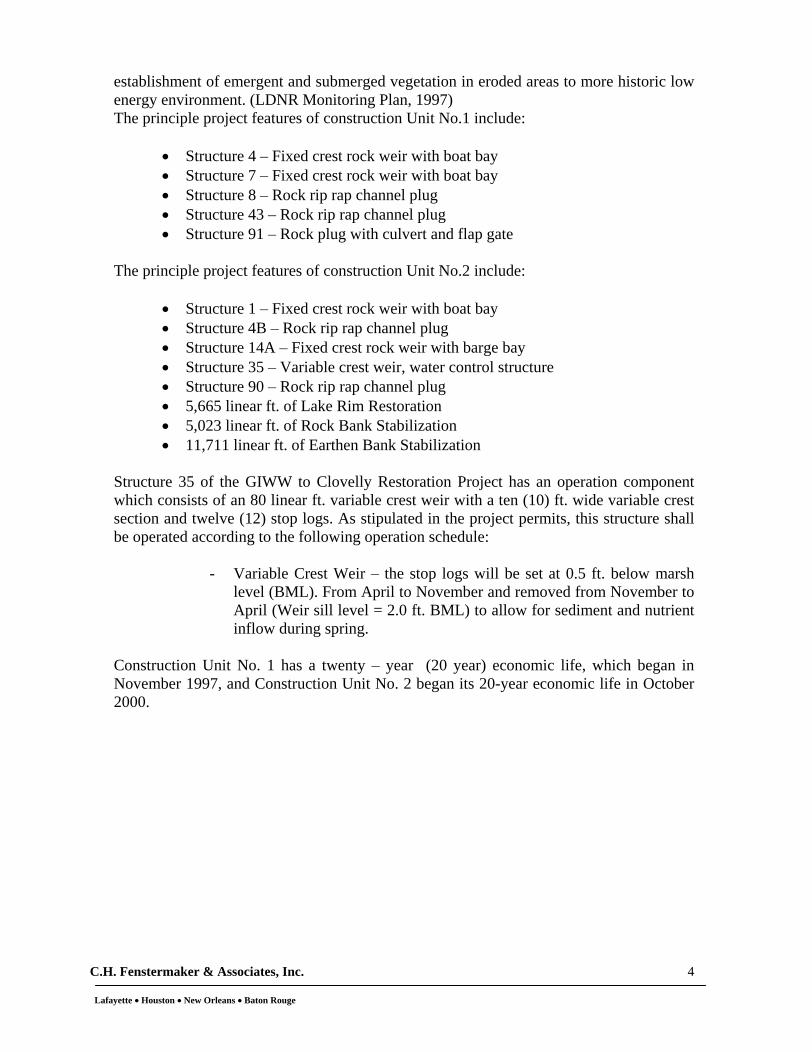
establishment of emergent and submerged vegetation in eroded areas to more historic low energy environment. (LDNR Monitoring Plan, 1997) The principle project features of construction Unit No.1 include:

Structure 4 Fixed crest rock weir with boat bay


Structure 8 Rock rip rap channel plug


Structure 91 Rock plug with culvert and flap gate

The principle project features of construction Unit No.2 include:


Structure 4B Rock rip rap channel plug

Structure 14A Fixed crest rock weir with barge bay

Structure 35 Variable crest weir, water control structure


5,665 linear ft. of Lake Rim Restoration

5,023 linear ft. of Rock Bank Stabilization

11,711 linear ft. of Earthen Bank Stabilization

Structure 35 of the GIWW to Clovelly Restoration Project has an operation component which consists of an 80 linear ft. variable crest weir with a ten (10) ft. wide variable crest section and twelve (12) stop logs. As stipulated in the project permits, this structure shall be operated according to the following operation schedule:

- Variable Crest Weir

the stop logs will be set at 0.5 ft. below marsh level (BML). From April to November and removed from November to April (Weir sill level = 2.0 ft. BML) to allow for sediment and nutrient inflow during spring.

Construction Unit No. 1 has a twenty

year (20 year) economic life, which began in November 1997, and Construction Unit No. 2 began its 20-year economic life in October 2000.



5

Figure 1.3: GIWW to Clovelly Hydrologic Restoration project features

1.4 ADAPTIVE ENVIRONMENTAL ASSESMENT AND MANAGMENT

The challenges associated with the management of large, complex ecosystems have led to the development of a management tool referred to as adaptive environemental assesment and management (AEAM) or simply, adaptive management.

The main goal of adaptive management is to achieve a management culture guided by an evoloving information system that is based on :

Observed ecosystem responses to past management activities

Modeled responses to potential future management alternatives

Monitoring information as well as directed research and modeling activites

N



6

A direct measurement of flows at any structure before and after construction under various hydrologic conditions would be helpful in determining the structure s effectiveness, but this is rarely performed. Computer simulations of the flows during the with and without project structures scenarious would also provide valuable insights. This is now usually done as part of the design process for all CWPPRA projects, however, in some of the earlier projects ( as the project being studied here; BA02 GIWW/Clovelly Hydrologic Restoration Project) this was not performed.2

The purpose of this study is as a part of the AEAM procedure is therfore to develop a computer simulation for one of the main structures of the BA-02 project the fixed-crest weir with barge bay on the Clovelly Canal ( Structure #14A shown in Figure 1.3 and 1.4) in order to estimate with and without weir water and salinity exchange at that site. This should provide valuable insight into the project effect on the saltwater intrusion.

The focus of the study is to assess the effectiveness of structure #14A, #43, #7 & #8 as shown in Figures 1.4 through 1.6

Figure 1.4: Structure #14A, the focus of this study

2 2004 Adaptive Management Environmental Assessment and Management. Draft Report for August 31, 2004 Workshop, Prepared by Bill Good, Ph.D. LA-Geological Survey.

Clovelly Canal

Little Lake

Location of Structure #14A

N



7

Figure 1.5: Structure #43

Figure 1.6: Structure #7 & #8

Detailed discussion of Model setup, calibration, and validation results is presented in Chapter Two.

Location of Structure #43

Structure #8

Structure #7

Little Lake

N

N



8

II. CHAPTER TWO

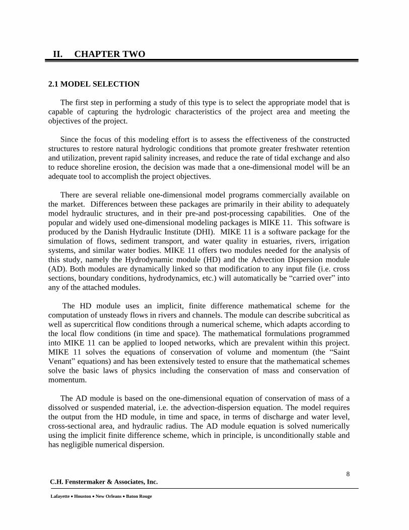
2.1 MODEL SELECTION

The first step in performing a study of this type is to select the appropriate model that is capable of capturing the hydrologic characteristics of the project area and meeting the objectives of the project.

Since the focus of this modeling effort is to assess the effectiveness of the constructed structures to restore natural hydrologic conditions that promote greater freshwater retention and utilization, prevent rapid salinity increases, and reduce the rate of tidal exchange and also to reduce shoreline erosion, the decision was made that a one-dimensional model will be an adequate tool to accomplish the project objectives.

There are several reliable one-dimensional model programs commercially available on the market. Differences between these packages are primarily in their ability to adequately model hydraulic structures, and in their pre-and post-processing capabilities. One of the popular and widely used one-dimensional modeling packages is MIKE 11. This software is produced by the Danish Hydraulic Institute (DHI). MIKE 11 is a software package for the simulation of flows, sediment transport, and water quality in estuaries, rivers, irrigation systems, and similar water bodies. MIKE 11 offers two modules needed for the analysis of this study, namely the Hydrodynamic module (HD) and the Advection Dispersion module (AD). Both modules are dynamically linked so that modification to any input file (i.e. cross sections, boundary conditions, hydrodynamics, etc.) will automatically be carried over into any of the attached modules.

The HD module uses an implicit, finite difference mathematical scheme for the computation of unsteady flows in rivers and channels. The module can describe subcritical as well as supercritical flow conditions through a numerical scheme, which adapts according to the local flow conditions (in time and space). The mathematical formulations programmed into MIKE 11 can be applied to looped networks, which are prevalent within this project. MIKE 11 solves the equations of conservation of volume and momentum (the Saint Venant equations) and has been extensively tested to ensure that the mathematical schemes solve the basic laws of physics including the conservation of mass and conservation of momentum.

The AD module is based on the one-dimensional equation of conservation of mass of a dissolved or suspended material, i.e. the advection-dispersion equation. The model requires the output from the HD module, in time and space, in terms of discharge and water level, cross-sectional area, and hydraulic radius. The AD module equation is solved numerically using the implicit finite difference scheme, which in principle, is unconditionally stable and has negligible numerical dispersion.



9

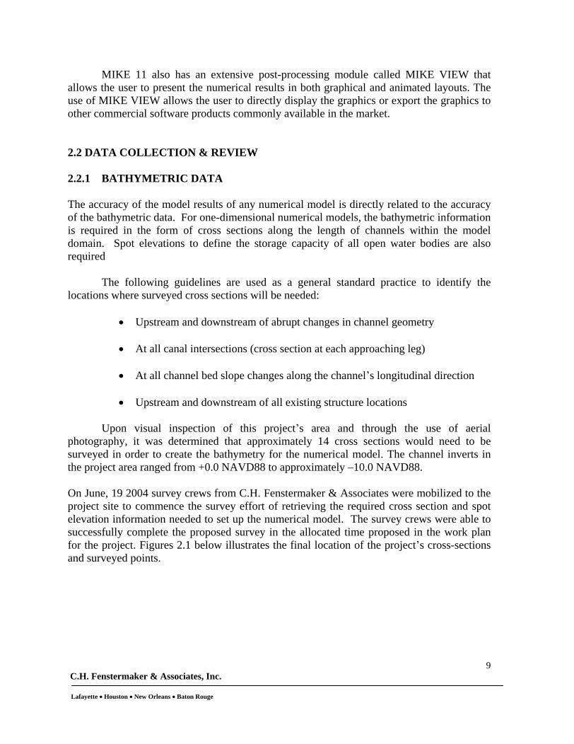
MIKE 11 also has an extensive post-processing module called MIKE VIEW that

allows the user to present the numerical results in both graphical and animated layouts. The use of MIKE VIEW allows the user to directly display the graphics or export the graphics to other commercial software products commonly available in the market.

2.2 DATA COLLECTION & REVIEW

2.2.1 BATHYMETRIC DATA

The accuracy of the model results of any numerical model is directly related to the accuracy of the bathymetric data. For one-dimensional numerical models, the bathymetric information is required in the form of cross sections along the length of channels within the model domain. Spot elevations to define the storage capacity of all open water bodies are also required

The following guidelines are used as a general standard practice to identify the locations where surveyed cross sections will be needed:

Upstream and downstream of abrupt changes in channel geometry

At all canal intersections (cross section at each approaching leg)

At all channel bed slope changes along the channel s longitudinal direction

Upstream and downstream of all existing structure locations

Upon visual inspection of this project s area and through the use of aerial photography, it was determined that approximately 14 cross sections would need to be surveyed in order to create the bathymetry for the numerical model. The channel inverts in the project area ranged from +0.0 NAVD88 to approximately 10.0 NAVD88.

On June, 19 2004 survey crews from C.H. Fenstermaker & Associates were mobilized to the project site to commence the survey effort of retrieving the required cross section and spot elevation information needed to set up the numerical model. The survey crews were able to successfully complete the proposed survey in the allocated time proposed in the work plan for the project. Figures 2.1 below illustrates the final location of the project s cross-sections and surveyed points.



10

Figure 2.1: Map Showing Location of Final Surveyed Points & Cross Sections.

Detailed information and dimensions of existing hydraulic structures were also surveyed. Survey crews were instructed to collect all possible information needed to accurately setup the model s structure components.

To streamline the survey effort for hydraulic structures, the field crews utilized coding techniques that are common in the surveying industry. Figures 2.2 through 2.4 describe the basic coding requirements for structures like or similar to the ones shown in these illustrations. Figure 2.5 shows a color photograph taken in the field for Structure 14A.



11

Figure 2.2: Basic Survey Coding for Weir Structure

Figure 2.3: Basic Survey Coding for Earthen or Rock Plug



12

Figure 2.4: Basic Survey Coding for Rock Weir Structure

Figure 2.5: Structure #14A (Fixed Crest rock weir with barge bay).



13

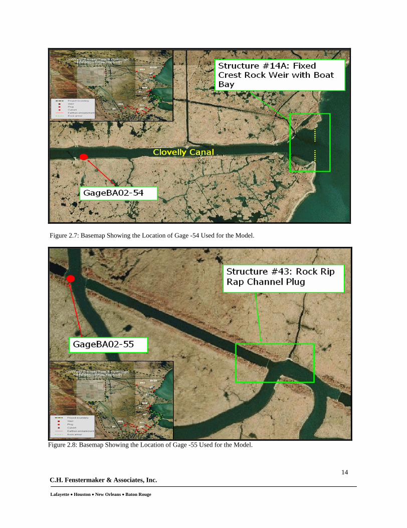
2.2.2 HYDROLOGIC DATA COLLECTION

Hydrologic field data are needed to setup the boundary conditions and to calibrate and validate the numerical model. The hydrologic parameters needed for this modeling effort are water level, discharge, and salinity.

Information from continuous recorders gauges 54, 55, 56, 58 and USGS gauge Little Lake near Cutoff

were used as boundary conditions and for the model s calibration and validation. Locations of all the gauges are shown in Figure 2.6 through 2.10.

Figure 2.6: Base map showing gauges used in the study



14

Figure 2.7: Basemap Showing the Location of Gage -54 Used for the Model.

Figure 2.8: Basemap Showing the Location of Gage -55 Used for the Model.



15

Figure 2.9: Base map Showing the Location of Gage - 58 Used for the Model.

Figure 2.10: Base map Showing the Location of Gage - 56 Used for the Model.



16

2.3 MODEL SETUP

The steps needed to set up the numerical model for this project includes:

1. Determining the extent of the numerical model domain. Care should be taken to ensure that:

The boundaries of the model extend beyond the area of interest.

The hydrologic or topographic adjustments and changes within the project area do not impact the conditions at the numerical model boundaries.

2. Setting up the channel network within the numerical model domain. (NOTE: In coastal Louisiana where a network of channels runs through the marsh, it is not practical to include all the channels as some are quite small in dimensions and do not carry or convey significant flow).

3. Assigning surveyed and estimated cross sections to all channels included in the model domain.

4. Include storage areas into the one-dimensional model if they exist. 5. Include all hydraulic structures within the numerical model domain. 6. Assign proper boundary conditions to each open end of every channel in the

numerical model domain.

It should be noted that the vertical datum for all the bathymetric data as well as the water level data was set to NAVD 88, while the horizontal datum was set to state plane coordinates Louisiana South Zone, NAD83.

2.3.1 SETUP OF CHANNEL NETWORK

The general layout of the channel network, boundaries, and hydraulic structures for the existing conditions are shown in Figures 2.11. An aerial is shown in the background of these figures to facilitate identifying the channels and their locations in the field.



17

Figure 2.11: Base map Showing MIKE 11 model network.

An extensive effort was made to ensure that the channel connectivity mimic the field conditions.

2.3.2 MODEL BOUNDARY CONDITIONS

The locations of the model boundaries are shown in Figure 2.6. A time series of hourly field measurements for water level and salinity is used as the boundary condition at each of these locations. Information relative to how the data was collected, reference datum, etc., can be found in Section 2.2.2.

2.3.3 MODELING OF HYDRAULIC STRUCTURES

There are numerous existing hydraulic structures within the project area that needed to be carefully modeled. A considerable amount of effort was devoted to ensure the accuracy of modeling all existing and proposed structures. The existing hydraulic structures typically found within the project site include:

Earthen plugs. These types of structures are fairly easy to model as long as the invert elevation of the plug is known

Rock weirs. These types of structures are fairly easy to model if the invert elevation and the dimensions are known. The flow over a broad crested weir is determined by the head differential between upstream and downstream

MIKE11 Channel



18

water levels, the geometry of the weir, and head losses. There are two regimes for flow over weirs (in addition to the trivial case of zero flow when the water levels are lower than the weir crest). These regimes are submerged or drowned flow, and free flow. Drowned flow, as the name indicates, occurs when the weir is submerged, i.e., when the flow is influenced by both the upstream and downstream water levels. The flow over a submerged or drowned weir can be expressed as follows:

21

))(( 211 hhZhbQ c

Where µ is the weir discharge coefficient h1 is the upstream water level h2 is the downstream water level Zc is the weir crest elevation

Free overflow, on the other hand, is controlled only by the upstream water level. The section where critical flow actually occurs, the velocity distribution, and the water level variations are the controlling factors that affect the discharge over a free flowing weir. The following equation (in System International, SI, units) can be used to describe a free flowing weir:

23

705.1 scc bHQ

Where c is the free overflow factor (a default value of 1.0 was used herein) Hs is the available energy head above the weir crest

For all the weirs modeled here, an entrance head loss factor of 0.5 and an exit head loss factor of 1.0 were used.

Variable crested weir. These types of structures are modeled as control structures. Knowledge of controlling factors for adjusting the crest elevation is required. MIKE11 requires a relationship between the controlling factor and the weir crest elevation.

2.4 MODEL CALIBRATION

Model calibration is defined as fine tuning of parameters until the numerical model produces results that mimic field measurements within an acceptable tolerance. These parameters may include bed-roughness coefficients, losses through hydraulic structures, diffusion coefficients, etc. The fine-tuning of these parameters should be physically based. In other words, numerical values assigned to these parameters should remain within the established range as documented in existing literature. A brief background about each calibration parameter is provided herein:



19

Friction Coefficient

B) 1-Dimensional model:

The channel s beds and banks and the marsh s surface cause friction losses to the energy of water flow. In the context of one-dimensional modeling, these losses are taken into account by the friction slope term in the momentum equation. In MIKE11, the bed-resistance term in the momentum equation is described as follows:

34

R

Q Q n 2

A

g

Where g is the gravitational acceleration, Q is the discharge, A is the cross sectional flow area, R is the hydraulic radius, and n is Manning s friction coefficient. The Manning n coefficient is used as one of the calibration parameters.

Dispersion Coefficient B) 1-Dimensional model:

The one-dimensional equation for conservation of mass of a constituent in a solution (such as temperature, salinity, etc) can be expressed as follows:

qCAKCx

CAD

xx

QC

t

AC.2

Where C is concentration (arbitrary unit), D is the dispersion coefficient, K is a linear decay coefficient, q is the lateral inflow, and C2 is source/sink concentration.

The dispersion coefficient is related to the cross sectional average velocity via the following relationship:

baVD

Where a and b are constants to be specified and they can be considered as additional calibration parameters.

Mixing Coefficient:

At an outflow (flow is leaving the numerical model domain) boundary, the concentration at the boundaries is calculated based on the concentration at the points neighboring that boundary, even if there is a time series of salinity



20

concentration specified at that boundary. At an inflow (flow is entering the numerical model domain) boundary, the concentration at the boundary is calculated as follows:

mixmixKtbfoutbf eCCCC

Where Cbf is the boundary concentration specified in the time series file, Cout

is the concentration at the boundary immediately before the flow direction changed (from outflow to inflow), Kmix is the time-scale mixing coefficient, and tmix is the time since the flow direction changed.

The parameters listed above were used as calibration parameters and were fine-tuned to achieve a good match between the numerical model results and the field data. The model was calibrated for the field data in the time period between November 01, 2002 and January 01, 2003. The following list shows values assigned to each of the three aforementioned parameters used to calibrate the model. These values produced a good match between the model results and the field data.

Manning s Friction Coefficient: 0.033 - 0.05

Mixing Coefficient Kmix: 0.5

Dispersion Coefficient (1D): - Dispersion factor a: 1.0 - Dispersion exponent b: 0.0

* It should be noted that the dispersion coefficient range in the 1-dimensional model was limited to a maximum of 100 m2/s and a minimum of 1 m2/s.

Water level and salinity calibration results in terms of Root Mean Square Deviations (RMSD) are shown below in table 2.1

RMSD RMSD RMSD RMSDppt % ft %

GAGE BA -02-54 1.64 10 0.2 5GAGE BA -02-55 1.64 13 0.1 7GAGE BA -02-56 1.57 10 0.16 6GAGE BA -02-58 1.53 9 0.12 3

SALINITY WATER LEVELSTATION

Table 2.1 Root mean square deviation calculations for water and salinity calibration results

As shown in the table, model results at three of the four stations have RMSD less than 10% and 6% for salinity and water level predictions, respectively. Overall, the statistical measures listed in Table 2.1 indicate that the model was able to simulate water levels and salinity values with a reasonable accuracy.



21

2.5. MODEL VALIDATION & EVALUATION OF MODEL PERFORMANCE

When the calibration process is complete, an independent data set is used to validate the model. The model was calibrated for the field data in the time period between November 01, 2002 and January 01, 2003. The data set that was used to validate the model extends to April 03, 2004. A detailed qualitative and quantitative analysis was performed to thoroughly assess the agreement and differences between model simulation results and actual field observations of both water level and salinity. The results of this analysis are presented in Figures 2.13-2.21 and Tables 2.2-2.7. In the following we present a brief explanation and discussion of these results:

Figures 2.13 and 2.14 show time-series of water level and salinity observations at one of the field stations (gauge BA-56) and the corresponding model results. The plotted time-series indicate that the model was able to capture the temporal magnitudes and patterns of salinity and water level changes.

Tables 2.2, 2.3, and 2.4 provide statistical quantification of model deviations in terms of three statistical measures: root mean square of deviations (RMSD), average of deviations (bias), and correlation coefficients. The computed statistics confirm the reasonable agreement between model results and the corresponding field measurements.

Figures 2.15 and 2.16 show the comparisons in the form of scatter plots. This form of comparison can reveal more details about the model predictions and their differences from actual observations, they could also be used to spot any erroneous data patterns as shown in Figure 2.15 at the lower end of gauge 54. The scatter plots show an overall good agreement.

Another way to assess the model accuracy is to calculate and plot the probability of exceedence functions (POE) shown in Figures 2.17 through 2.19. In these functions, the salinity (or water level) value that corresponds to a certain probability of exceedence (e.g., 5%) is calculated. Each point in the figure represents the probability that a certain salinity (or water level) value will be exceeded. Rather than focusing on comparisons of individual points, the POE plots provide a good assessment of the agreement between distributions of model predictions and field observations. The plots indicate that, for most of the gauges, the model was able to reproduce the overall distributions of water levels and salinities with a reasonable accuracy.

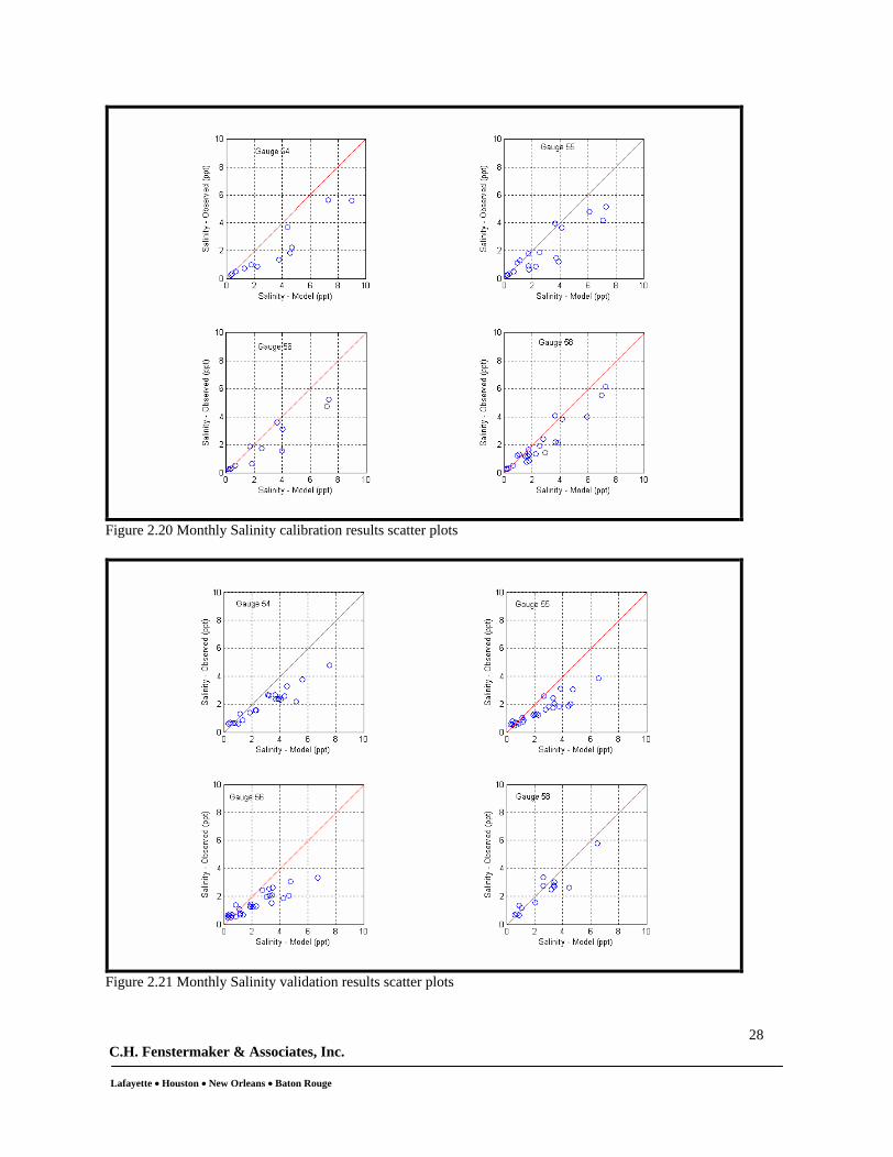
Besides the hourly time scale, model results were also evaluated after being aggregated to monthly averages. Monthly time scale is also important since salinity variations and water level inundations become more significant if they persist for longer periods. The above analyses were repeated for a monthly scale and some example results are shown in Figures 2.20 and 2.21 and Tables 2.5-2.7. Some of the analyzed gauges showed slight levels of biases. However, the results show an overall good performance agreement at monthly scales. It should be noted that some of the observed disagreement can be attributed to the relatively small sample sizes available at monthly scales.



22

2.6. DISCUSSION OF LIMITATIONS AND CAPABILITIES OF THE MODEL

One-dimensional models, in general, do not provide information of salinity distribution across the width of a channel or over the water column of that channel. Rather, it provides a cross-section salinity average. A one-dimensional model assumes that the salinity is mixed over any given channel cross section. One-dimensional models, however, do provide for the changes in salinity from one station to another along the length of a channel. For this particular project, the channels are fairly small and shallow, therefore, flow stratification is minimal and the variation of salinity from one bank of a channel to the other is small. It is for this reason that a one-dimensional model can be used.

It should also be noted here that the decision was made to include only the northern part of BA-02 up to structure 7 shown in Figure 2.12. All the structures south of structure 7 were excluded from this modeling study, as it was determined by all the contracting agencies that a hydrologic barrier exist at this area, making the two sets of structures to act independently from each other.

Figure 2.12: Hydrologic Barrier in BA-02

Hydrologic Barrier



23

Water Level at gauge BA-56

-0.4

-0.2

0.0

0.2

0.4

0.6

0.8

1.0

1.2

1.4

1.6

1/1/01 7/20/01 2/5/02 8/24/02 3/12/03 9/28/03

Time

Wat

er L

evel

(m

)

BA56 Sim at BA56

Figure 2.13: Water Level validation results at gauge 56

Sal at gauge BA-56

0.0

2.0

4.0

6.0

8.0

10.0

12.0

14.0

16.0

18.0

20.0

1/1/01 7/20/01 2/5/02 8/24/02 3/12/03 9/28/03

Time

Sal

init

y (p

pt)

BA56 Sim at BA56

Figure 2.14: Salinity validation results at gauge 56



24

RMSD RMSD RMSD RMSD

ppt % ft %GAGE BA -02-54 1.61 11 0.21 4GAGE BA -02-55 1.43 15 0.17 4GAGE BA -02-56 1.53 16 0.2 5GAGE BA -02-58 1.82 12 0.16 3


Table 2.2 Root mean square deviation calculations for water and salinity validation results

Calibration Validation Calibration Validation

GAGE BA -02-54 1.37 0.84 0.06 0.12GAGE BA -02-55 0.89 0.74 0.03 0.36GAGE BA -02-56 0.9 0.73 -0.1 0.11GAGE BA -02-58 0.66 0.3 0.08 0.27


ppt ft

Table 2.3 Bias calculations for water and salinity results

Calibration Validation Calibration ValidationGAGE BA -02-54 0.84 0.8 0.95 0.94GAGE BA -02-55 0.76 0.66 0.9 0.94GAGE BA -02-56 0.79 0.71 0.91 0.93GAGE BA -02-58 0.8 0.7 0.98 0.98


Table 2.4 Model Correlations calculations for simulated water and salinity results vs. observed data

Observed Model Observed Model

GAGE BA -02-54 20 17 31 31GAGE BA -02-55 19 13 14 30GAGE BA -02-56 34 18 30 29GAGE BA -02-58 7 6.5 3 5

STATIONCalibration Validation

%

Exceedence Frequency

Table 2.5 Frequency of Exceedence results (assumed marsh elevation = 1.2 ft)



25


GAGE BA -02-54 58 58 72 77GAGE BA -02-55 61 56 65 69GAGE BA -02-56 59 50 66 69GAGE BA -02-58 70 74 79 64


%

SALINITY THRESHOLD (0-6 PPT)

Table 2.6 Monthly Salinity switcher threshold results


GAGE BA -02-54 100 83 100 95GAGE BA -02-55 100 83 100 96GAGE BA -02-56 100 83 100 97GAGE BA -02-58 96 96 100 93


%

SALINITY THRESHOLD (0-6 PPT)

Table 2.7 Monthly Salinity switcher threshold results

Figure 2.15 Scatter Plots for water level calibration results

Small Sample Size

Small Sample Size



26

Figure 2.16 Scatter Plots for water level validation results

Figure 2.17 water level calibration results distributions



27

Figure 2.18 water level validation results distributions

Figure 2.19 Salinity validation results distributions



28

Figure 2.20 Monthly Salinity calibration results scatter plots

Figure 2.21 Monthly Salinity validation results scatter plots


Lafayette Baton Rouge New Orleans Houston Nashville

29

III. CHAPTER THREE

3.1 ANALYSIS OF MODEL RESULTS

After consulting with the state and federal agencies, the following four additional model scenarios were simulated using the validated model:

Scenario # 1: None Model simulation with removing all the constructed structures from the channel network (Pre construction case)

Scenario # 2: ALL Model simulation with all the constructed structures from the channel network (Existing conditions case)

Scenario # 3: ALL-14A Model simulation with all the constructed structures except structure 14A

Scenario # 4: ALL with14A modified

Model simulations with all the constructed structures and modifying structure 14A as shown in Figure 3.1 [Raising the invert to elevation -5 ft NAVD 88 and decreasing bottom width to 40 ft]

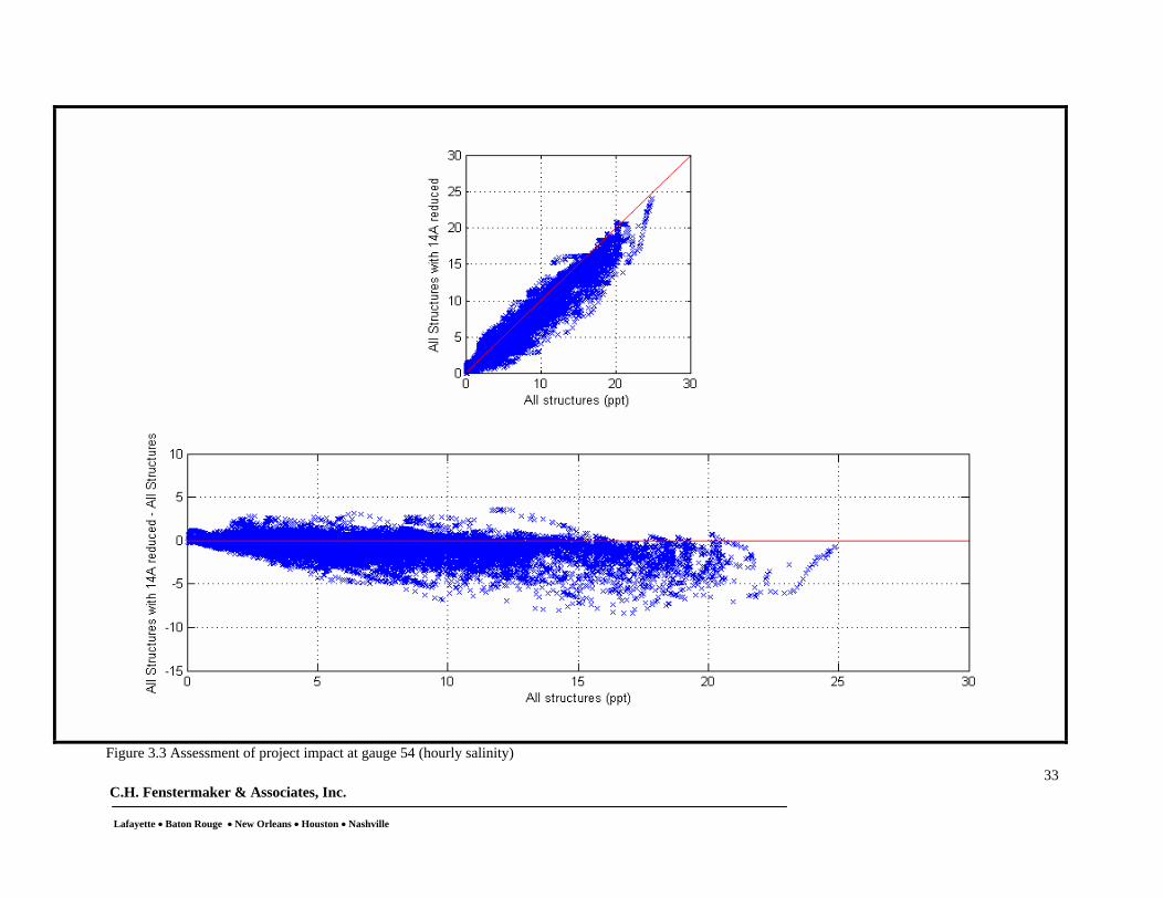
The purpose of these simulations was to effectively evaluate the effect of the structures on the surrounding marshes. Evaluation of model results for the first three scenarios with respect to the None base case, and with respect to each other, would give insight about their relative impacts on the salinity and water level changes in the project area. Assessment of each pair of scenarios is presented in the following form:

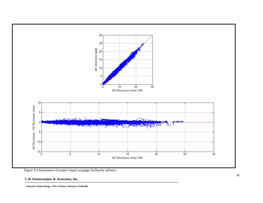
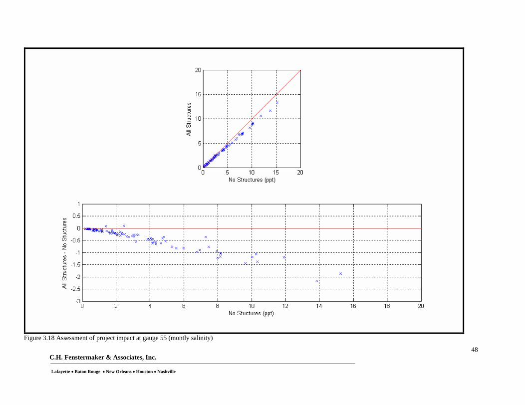
Scatter plot of salinity values of one scenario versus the other

Scatter plot of the salinity differences between the two scenarios versus the corresponding salinity magnitude of one of the two scenarios.

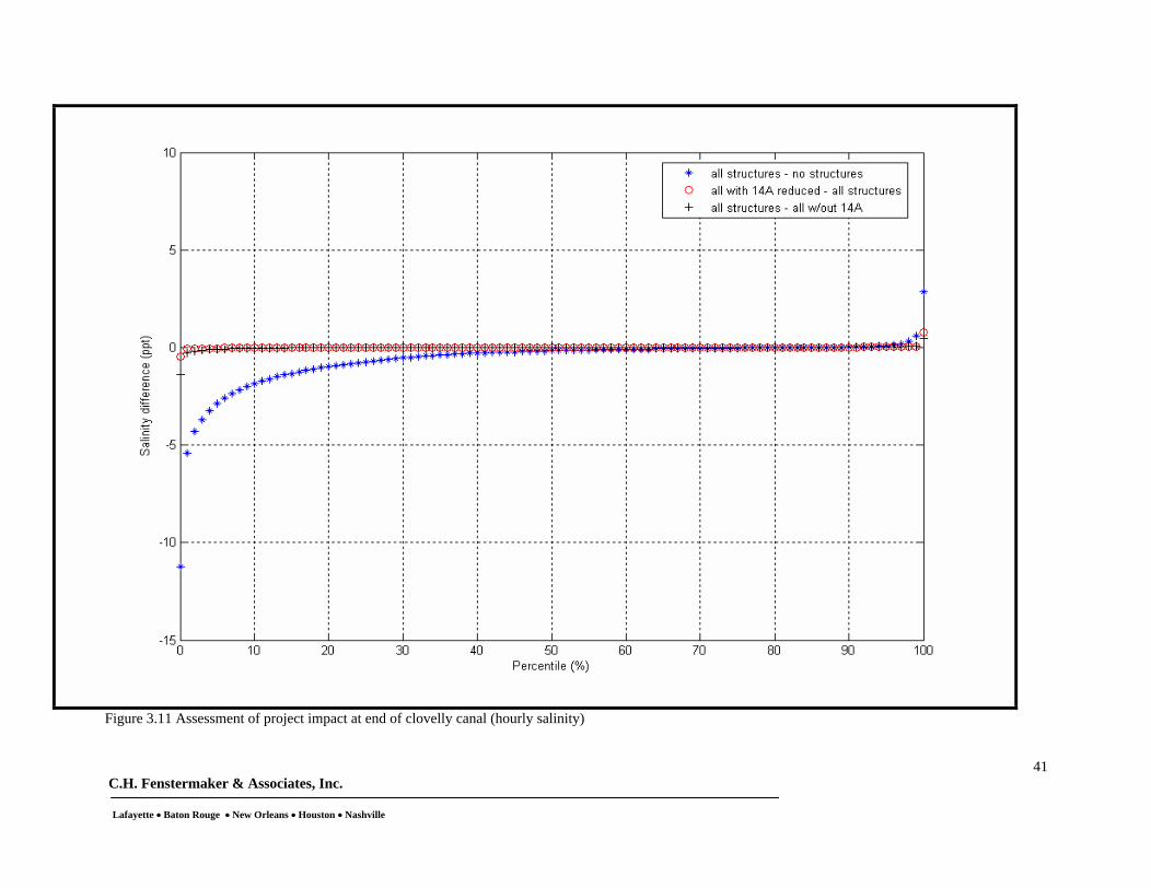
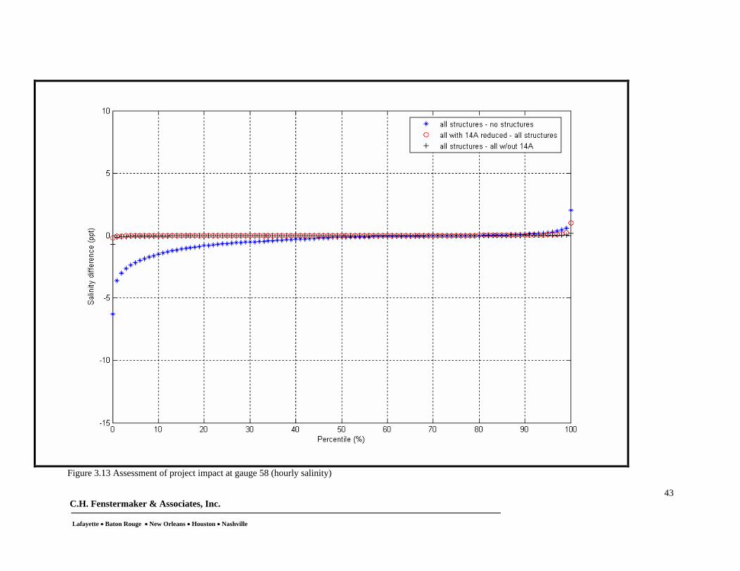
In addition, differences between each two scenarios are also analyzed by computing their probability of exceedence functions.

The analysis was performed for both hourly and monthly time scales and example results are summarized in Figures 3.2 to 3.21 for selected gauge locations. The following set of remarks can be made about the results:

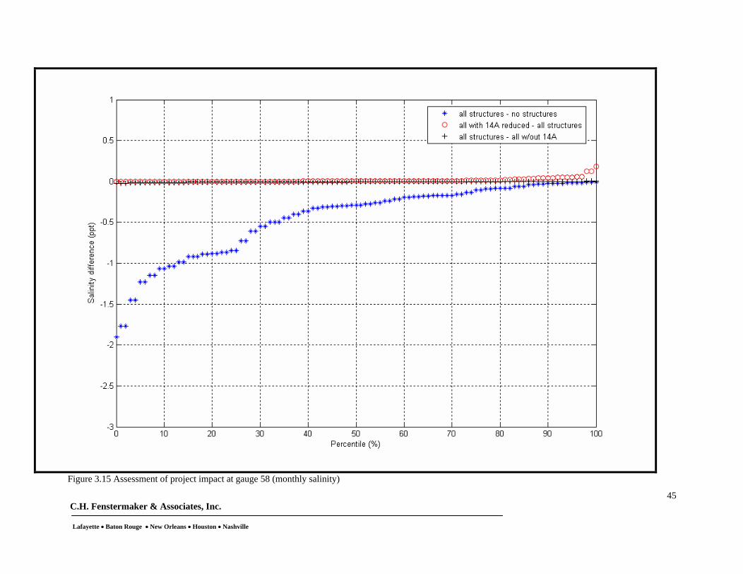
The most impact on salinity values of the base simulation is obtained with scenario # 2 which includes all of the constructed structures. Significant salinity reductions as high as 10 and 2.5 ppt are reported at hourly and monthly scales, respectively.

Comparing scenario # 3 versus scenarios # 1 and 2 indicates that including all structures except structure 14A was still effective in reducing hourly and salinity magnitudes.

Despite the minor contribution of structure 14A, further salinity reductions were observed as a result of decreasing its size. However, it should be noted that such



30

further reductions in the salinity levels were limited to the proximity of structure 14A. Analysis at other locations farther from structure 14A (not shown herein) indicated minor impact in terms of salinity reductions.

Modified Size of Structure 14A

-10

-8

-6

-4

-2

0

2

4

6

0 200 400 600 800 1000 1200

Station(ft)

Ele

vati

on

(N

AV

D88

-ft)

Existing 14A Modified 14A

Figure 3.1 Reduced size for Structure 14A

3.2 FINAL CONCLUSIONS AND CLOSING REMARKS

The modeling effort presented in this study was aimed to evaluate the performance of the existing structures for BA-02. A one-dimensional (MIKE 11) computer model was used to perform the evaluation the performance of the existing structures. The model was able to capture water level and salinity variations in the project channels network.

The overall conclusions of this study are summarized below:

North of Clovelly Canal (Gauge BA-56): The model results showed that installing the structures does not have an impact on the salinity reduction north of the Clovelly canal due to the existing ground slope in the project area (a decreasing slope southwards) forcing the water to flow from north to south.



31

South of Clovelly Canal:

The model results illustrated that having all the structures in place reduced salinity in the project area (in the magnitude of 3-4 ppt on average at gauge 55 and 58). Structure 14A appears to have only a local effect in the Clovelly Canal around the structure itself. Having the structure in place reduced the salinity in the Clovelly canal (4 -5 ppt at gauge 54).

Reducing the size of structure 14A provided additional salinity reduction (an additional 2-3 ppt at gauge 54). However this additional salinity reduction was not noticed on the southern portion of the project (gauge 55 and 58). This salinity reduction was noticed on the hourly scale and also the monthly scale.



32

Figure 3.2 Assessment of project impact at gauge 54 (hourly salinity)



33




34




35




36

Figure 3.6 Assessment of project impact at gauge 54 (monthly salinity)



37




38




39




40

Figure 3.10 Assessment of project impact at end of clovelly canal (hourly salinity)



41




42




43




44




45




46




47




48

Figure 3.18 Assessment of project impact at gauge 55 (montly salinity)



49




50




51


ba-02 giww/clovelly

Documents