b206 [email protected] 201-216-5549personal.stevens.edu/~bmcnair/ee359-s10/lecture 19.pdf ·...
TRANSCRIPT


2
Memory and AdvancedDigital Circuits
Chapter 11

3
Figure 11.1 (a) Basic latch. (b) The latch with the feedback loop opened. (c) Determining the operating point(s) of the latch.

4
Figure 11.2 (a) The set/reset (SR) flip-flop and (b) its truth table.

5
Figure 11.3 CMOS implementation of a clocked SR flip-flop. The clock signal is denoted by .

6
Figure 11.4 The relevant portion of the flip-flop circuit of Fig. 11.3 for determining the minimum W/L ratios of Q5 and Q6 needed to ensure that the flip-flop will switch.

7
Figure 11.5 A simpler CMOS implementation of the clocked SR flip-flop. This circuit is popular as the basic cell in the design of static random-access memory (SRAM) chips.

8
Figure 11.6 A block-diagram representation of the D flip-flop.

9
Figure 11.7 A simple implementation of the D flip-flop. The circuit in (a) utilizes the two-phase nonoverlapping clock whose waveforms are shown in (b).

10
Figure 11.8 (a) A master–slave D flip-flop. The switches can be, and usually are, implemented with CMOS transmission gates. (b) Waveforms of the two-phase nonoverlapping clock required.

11
Figure 11.9 The monostable multivibrator (one-shot) as a functional block, shown to be triggered by a positive pulse. In addition, there are one shots that are triggered by a negative pulse.

12
Figure 11.10 A monostable circuit using CMOS NOR gates. Signal source vI supplies positive trigger pulses.

13
Figure 11.11 (a) Diodes at each input of a two-input CMOS gate. (b) Equivalent diode circuit when the two inputs of the gate are joined together. Note that the diodes are intended to protect the device gates from potentially destructive overvoltages due to static charge accumulation.

14
Figure 11.12 Output equivalent circuit of CMOS gate when the output is (a) low and (b) high.

15
Figure 11.13 Timing diagram for the monostable circuit in Fig. 11.10.

16
Figure 11.14 Circuit that applies during the discharge of C (at the end of the monostable pulse interval T).

17
Figure 11.15 (a) A simple astable multivibrator circuit using CMOS gates. (b) Waveforms for the astable circuit in (a). The diodes at the gate input are assumed to be ideal and thus to limit the voltage vI1 to 0 and VDD.

18
Figure 11.16 (a) A ring oscillator formed by connecting three inverters in cascade. (Normally at least five inverters are used.) (b) The resulting waveform. Observe that the circuit oscillates with frequency 1/6tP.

19
Figure 11.17 A 2M+N-bit memory chip organized as an array of 2M rows 2N columns.

20
Figure 11.18 A CMOS SRAM memory cell.
21
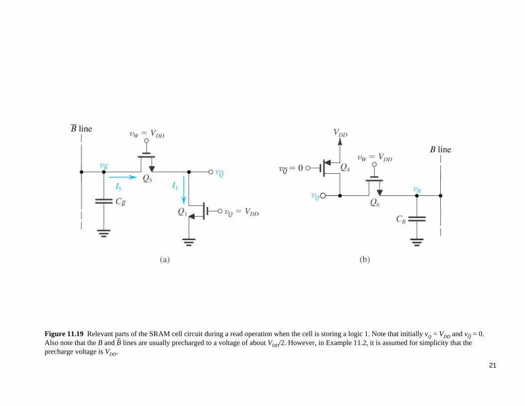
Figure 11.19 Relevant parts of the SRAM cell circuit during a read operation when the cell is storing a logic 1. Note that initially vQ = VDD and vQ = 0. Also note that the B and B lines are usually precharged to a voltage of about VDD/2. However, in Example 11.2, it is assumed for simplicity that the precharge voltage is VDD.

22
Figure 11.20 Relevant parts of the SRAM circuit during a write operation. Initially, the SRAM has a stored 1 and a 0 is being written. These equivalent circuits apply before switching takes place. (a) The circuit is pulling node Q up toward VDD/2. (b) The circuit is pulling node Q down toward VDD/2.

23
Figure 11.21 The one-transistor dynamic RAM cell.

24
Figure 11.22 When the voltage of the selected word line is raised, the transistor conducts, thus connecting the storage capacitor CS to the bit-line capacitance CB.

25
Figure 11.23 A differential sense amplifier connected to the bit lines of a particular column. This arrangement can be used directly for SRAMs (which utilize both the B and B lines). DRAMs can be turned into differential circuits by using the “dummy cell” arrangement shown in Fig. 11.25.

26
Figure 11.24 Waveforms of vB before and after the activation of the sense amplifier. In a read-1 operation, the sense amplifier causes the initial small increment V(1) to grow exponentially to VDD. In a read-0 operation, the negative V(0) grows to 0. Complementary signal waveforms develop on the B line.

27
Figure 11.25 An arrangement for obtaining differential operation from the single-ended DRAM cell. Note the dummy cells at the far right and far left.

28
Figure 11.26 A NOR address decoder in array form. One out of eight lines (row lines) is selected using a 3-bit address.

29
Figure 11.27 A column decoder realized by a combination of a NOR decoder and a pass-transistor multiplexer.

30
Figure 11.28 A tree column decoder. Note that the colored path shows the transistors that are conducting when A0 = 1, A1 = 0, and A2 = 1, the address that results in connecting B5 to the data line.

31
Figure 11.29 A simple MOS ROM organized as 8 words 4 bits.

32
Figure 11.30 (a) Cross section and (b) circuit symbol of the floating-gate transistor used as an EPROM cell.

33
Figure 11.31 Illustrating the shift in the iD–vGS characteristic of a floating-gate transistor as a result of programming.

34
Figure 11.32 The floating-gate transistor during programming.

35
Figure 11.33 The basic element of ECL is the differential pair. Here, VR is a reference voltage.

36
Figure 11.34 Basic circuit of the ECL 10K logic-gate family.

37
Figure E11.18

38
Figure 11.35 The proper way to connect high-speed logic gates such as ECL. Properly terminating the transmission line connecting the two gates eliminates the “ringing” that would otherwise corrupt the logic signals. (See Section 11.7.6.)
39
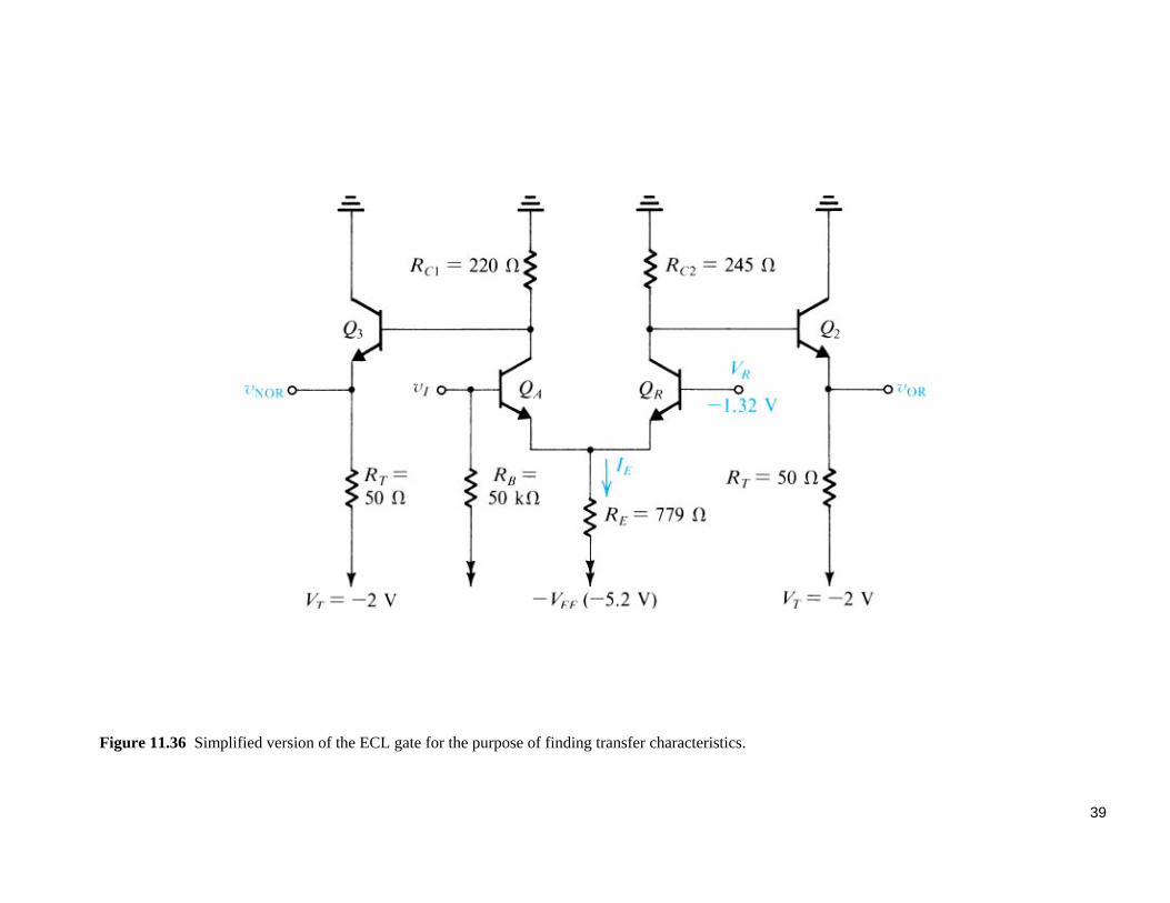
Figure 11.36 Simplified version of the ECL gate for the purpose of finding transfer characteristics.

40
Figure 11.37 The OR transfer characteristic vOR versus vI , for the circuit in Fig. 11.36.

41
Figure 11.38 Circuit for determining VOH.

42
Figure 11.39 The NOR transfer characteristic, vNOR versus vI , for the circuit in Fig. 11.36.

43
Figure 11.40 Circuit for finding, vNOR versus vI for the range vI > VIH.

44
Figure 11.41 Equivalent circuit for determining the temperature coefficient of the reference voltage VR .

45
Figure 11.42 Equivalent circuit for determining the temperature coefficient of VOL.

46
Figure 11.43 Equivalent circuit for determining the temperature coefficient of VOH.

47
Figure 11.44 The wired-OR capability of ECL.

48
Figure 11.45 Development of the BiCMOS inverter circuit. (a) The basic concept is to use an additional bipolar transistor to increase the output current drive of each of QN and QP of the CMOS inverter. (b) The circuit in (a) can be thought of as utilizing these composite devices.

49
Figure 11.45 (Continued) (c) To reduce the turn-off times of Q1 and Q2, “bleeder resistors” R1 and R2 are added. (d) Implementation of the circuit in (c) using NMOS transistors to realize the resistors. (e) An improved version of the circuit in (c) obtained by connecting the lower end of R1 to the output node.

50
Figure 11.46 Equivalent circuits for charging and discharging a load capacitance C. Note that C includes all the capacitances present at the output node.

51
Figure 11.47 A BiCMOS two-input NAND gate.

52
Figure 11.48 Capture schematic of the two-input ECL gate for Example 11.5.

53
Figure 11.49 Circuit arrangement for computing the voltage transfer characteristics of the ECL gate in Fig. 11.48.

54
Figure 11.50 Voltage transfer characteristics of the OR and NOR outputs (see Fig. 11.49) for the ECL gate shown in Fig. 11.48. Also indicated is the reference voltage, VR = –1.32 V.

55
Figure 11.51 Comparing the voltage transfer characteristics of the OR and NOR outputs (see Fig. 11.49) of the ECL gate shown in Fig. 11.48, with the reference voltage VR generated using: (a) the temperature-compensated bias network of Fig. 11.48.

56
Figure 11.51 (Continued) (b) a temperature-independent voltage source.
57
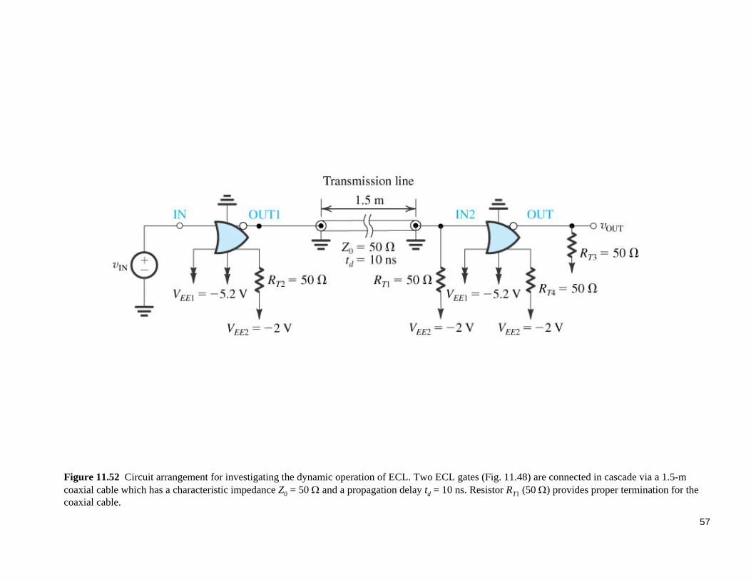
Figure 11.52 Circuit arrangement for investigating the dynamic operation of ECL. Two ECL gates (Fig. 11.48) are connected in cascade via a 1.5-m coaxial cable which has a characteristic impedance Z0 = 50 and a propagation delay td = 10 ns. Resistor RT1 (50 ) provides proper termination for the coaxial cable.

58
Figure 11.53 Transient response of a cascade of two ECL gates interconnected by a 1.5-m coaxial cable having a characteristic impedance of 50 and a delay of 10 ns (see Fig. 11.52).
59
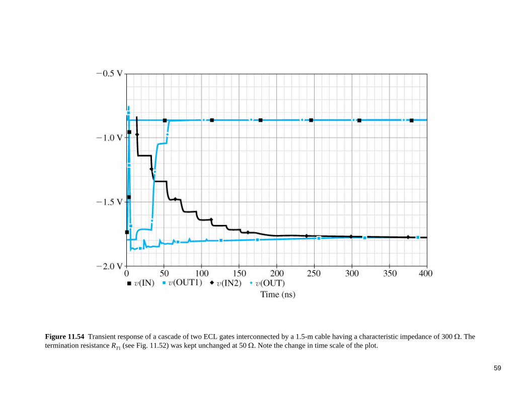
Figure 11.54 Transient response of a cascade of two ECL gates interconnected by a 1.5-m cable having a characteristic impedance of 300 . The termination resistance RT1 (see Fig. 11.52) was kept unchanged at 50 . Note the change in time scale of the plot.

60
Figure P11.40

61
Figure P11.50