b-spline finite elements and their efficiency in solving ... · b-spline finite elements and their...
TRANSCRIPT

arX
iv:n
ucl-
th/9
8080
66v1
26
Aug
199
8
B-Spline Finite Elements and their Efficiency in Solving
Relativistic Mean Field Equations
W. PoschlPhysics-Department of the Duke University,
Durham, NC-27708, USA(December 14, 2017)
A finite element method using B-splines is presented and compared with a conventional fi-nite element method of Lagrangian type. The efficiency of both methods has been investigatedat the example of a coupled non-linear system of Dirac eigenvalue equations and inhomogeneousKlein-Gordon equations which describe a nuclear system in the framework of relativistic mean fieldtheory. Although, FEM has been applied with great success in nuclear RMF recently, a well knownproblem is the appearance of spurious solutions in the spectra of the Dirac equation. The question,whether B-splines lead to a reduction of spurious solutions is analyzed. Numerical expenses, preci-sion and behavior of convergence are compared for both methods in view of their use in large scalecomputation on FEM grids with more dimensions. A B-spline version of the object oriented C++code for spherical nuclei has been used for this investigation.
PROGRAM SUMMARY
Title of program: bspFEM.cc
Catalogue number : ..........
Program obtainable from:
Computer for which the program is designed and others on which it has been tested : any Unix work-station.
Operating system: Unix
Programming language used : C++
No. of lines in combined program and test deck :
Keywords: B-splines, Finite Element Method, Lagrange type shape functions, relativistic mean-field theory, mean-fieldapproximation, spherical nuclei, Dirac equations, Klein-Gordon equations, classes
Nature of physical problemThe ground-state of a spherical nucleus is described in the framework of relativistic mean field theory in coordinatespace. The model describes a nucleus as a relativistic system of baryons and mesons. Nucleons interact in a relativisticcovariant manner through the exchange of virtual mesons: the isoscalar scalar σ-meson, the isoscalar vector ω-mesonand the isovector vector ρ-meson. The model is based on the one boson exchange description of the nucleon-nucleoninteraction.
Method of solutionAn atomic nucleus is described by a coupled system of partial differential equations for the nucleons (Dirac equations), anddifferential equations for the meson and photon fields (Klein-Gordon equations). Two methods are compared which allowa simple, self-consistent solution based on finite element analysis. Using a formulation based on weighted residuals, thecoupled system of Dirac and Klein-Gordon equations is transformed into a generalized algebraic eigenvalue problem, and
1

systems of linear and nonlinear algebraic equations, respectively. Finite elements of arbitrary order are used on uniformradial mesh. B-splines are used as shape functions in the finite elements. The generalized eigenvalue problem is solvedin narrow windows of the eigenparameter using a highly efficient bisection method for band matrices. A biconjugategradient method is used for the solution of systems of linear and nonlinear algebraic equations.
Restrictions on the complexity of the problemIn the present version of the code we only consider nuclear systems with spherical symmetry.
LONG WRITE-UP
I. INTRODUCTION
Over the last decade, the relativistic mean field theory (RMF) has been applied with great successto the description of low energy properties of nuclei [2,1] and to the description of scattering atintermediate energies []. Therefore, RMF gains increasing recognition. Effective models have beensuggested [3,1] which are represented by Lagrangians containing both, nucleonic and mesonic fieldswith coupling constants that have been adjusted to the many body system of nuclear matter and tofinite nuclei in the valley of β-stability [4,5]. Of course, such a procedure is completely phenomeno-logical and in spirit very similar to the non-relativistic density dependent HF-models (DDHF) ofSkyrme and Gogny [6,7]. Compared to DDHF theory, the relativistic models seem to have impor-tant advantages: (i) they start on a more fundamental level, treating mesonic degrees explicitly andallowing a natural extension for heavy-ion reactions with higher energies, (ii) they incorporate fromthe beginning important relativistic effects, such as the existence of two types of potentials (scalarand vector) and the resulting strong spin-orbit term, a new saturation mechanism by the relativisticquenching of the attractive scalar field and the existence of anti-particle solutions, (iii) finally theyare in many respects easier to handle than non-relativistic DDHF calculations.
Since the discovery of the halo phenomenon in light drip-line nuclei [8] the study of the structureof exotic nuclei has become a very exciting topic. Experiments with radioactive beams provide a lotof new data over entirely new (”exotic”) regions of the chart of nuclides. On the theoretical side,presently existing models of the nucleus, relativistic ones as well as non-relativistic ones, have to betested in these new regions in comparison with experiment. Improvements and extensions of themodels become necessary.
Recent investigations [9,10] have shown that coupling to the particle continuum and large exten-sions in coordinate space have to be taken into account in order to describe phenomena of exoticnuclear structure. The underlying equations of all nuclear models have therefore to be solved ondiscretizations in coordinate space. In contrast to ”conventional” methods, based on expansions ofthe solution in basis functions with spherical or axial symmetry, sophisticated techniques have tobe applied in order to solve the mean field equations in coordinate space.
With the non-relativistic HF-models extensive nuclear structure calculations have been performedbased on the imaginary time method [11]. This very efficient method, however, is restricted tothe non-relativistic cases where the single particle spectrum is limited from below. In relativisticmodel calculations, the imaginary time method would not converge due to mixing with negativeenergy states. Therefore, we plan a different approach with Krylov-subspace based methods [12](for solutions on 2D and 3D meshes in coordinate space) and with the bisection method (1D sphericalcase [14]). In contrast to the imaginary time method, the required single particle or quasi particleeigenstates have to be calculated in each step of a self-consistent iteration. At first sight, it seems,that this approach is intractable since coordinate space discretizations on 2D or 3D finite elementmeshes lead to eigenvalue problems of large dimensions. With the block Lanczos method however,the calculation of eigenvalues and corresponding eigenvectors can be restricted to a small numberwhich is required in the region of bound nucleons. In combination with the selfconsistent iterationmethod which is applied to the whole problem, the number of internal block Lanczos iterations can bereduced to corrections of the vectors which come from the previous iterations step of the selfconsistentloop. In references [13,14] the solution of the spherical RMF equations and the spherical RHBequations with the finite element method in coordinate space has been demonstrated. In theseinvestigations, I have observed that spurious solutions appear in the spectrum of eigenvalues of theDirac operator of the RHB equations when they are discretized with finite elements of the Lagrangiantype. Since the numerical cost to calculate eigensolutions on 1D-meshes is relatively small, it was notimportant to avoid spurious solutions a priori and therefore they have been eliminated by comparison
2

of the number of nodes. In the 2D and 3D cases, however, it is important to reduce the size of thestiffness matrices to a minimum. This can be achieved by using shape functions with extremelygood properties of interpolation, allowing wider meshes in coordinate space. Since B-splines aresmooth, one would expect that they have the desired properties.
The major goal of the present paper is to give an answer to the question whether B-splines canimprove the numerics in comparison to the often used shape functions of Lagrangian type. At thepresent state, our study is restricted to the solution of relativistic mean field equations. The resultsof our investigation are important with respect to large scale computations on finite element meshesof two and three dimensions. Such calculations are required in the relativistic mean field descriptionof deformed exotic nuclei at low energies. I have worked out a B-spline version of the computer codewhich is published in [14] and compare the results obtained with both codes for spherical nuclei.
II. THE RELATIVISTIC MEAN FIELD EQUATIONS
The relativistic mean field model describes the nucleus as a system of nucleons which interactthrough the exchange of virtual mesons: the isoscalar scalar σ-meson, the isoscalar vector ω-mesonand the isovector vector ρ-meson. The model is based on the one boson exchange description of thenucleon-nucleon interaction. The effective Lagrangian density is [3]
L = ψ (iγ · ∂ −m)ψ
+1
2(∂σ)2 − U(σ)−
1
4ΩµνΩ
µν +1
2m2
ωω2 −
1
4~Rµν
~Rµν +1
2m2
ρ~ρ2 −
1
4FµνF
µν
−gσψσψ − gωψγ · ωψ − gρψγ · ~ρ~τψ − eψγ ·A(1− τ3)
2ψ . (1)
Vectors in isospin space are denoted by arrows. The Dirac spinor ψ denotes the nucleon with massm. mσ, mω, and mρ are the masses of the σ-meson, the ω-meson, and the ρ-meson. gσ, gω, and gρare the corresponding coupling constants for the mesons to the nucleon. e2/4π = 1/137.036.
Since the relativistic mean field model has been described in a large number of articles, I omit along discussion of the above given Lagrangian and the derivation of the RMF equations. Instead,I refer to section 2 of reference [13] and to section 2 of reference [14]. In these references, thedevelopment preceding to the investigations of the present paper is described in details. The maininterest of the work presented below is focused on numerical aspects and performance of two FEMtechniques in the solution of the RMF equations for spherical nuclei. In the following, I briefly listthe static RMF equations for the spherical symmetric case.
Introducing spherical polar coordinates (r, θ, φ), the Dirac equation reduces to a set of two coupledordinary differential equations for the amplitudes g(r) and f(r) for proton and neutron states
(
∂r +κ+ 1
r
)
g(r) +(
m+ S(r)− V (r))
f(r) = −ε fi(r),
(
∂r −κ− 1
r
)
f(r) +(
m+ S(r) + V (r))
g(r) = +ε g(r), (2)
where the quantum number κ = ±1,±2,±3, .... The scalar potential S(r) and the vector potentialV (r) are composed of boson field amplitudes and coupling constants where
S(r) = gσ σ(r), (3)
and
V (r) = gω ω0(r) + gρ τ3 ρ
03(r) + e
(1− τ3)
2A0(r). (4)
The symbols gσ, gω, gρ, and e denote the coupling constants of the σ-field, the ω-field, the ρ-fieldand the A-field, coupled to the nucleons. The meson fields σ(r), ω0(r), ρ03(r) and the photon fieldA0(r) are solutions of the inhomogeneous Klein-Gordon equations
(
−∂2r −
2
r∂r +
l(l + 1)
r2+m2
σ
)
σ(r) = −gσ ρs(r)− g2 σ2(r)− g3 σ
3(r) (5)
(
−∂2r −
2
r∂r +
l(l + 1)
r2+m2
ω
)
ω0(r) = gω ρv(r) (6)
3
(
−∂2r −
2
r∂r +
l(l + 1)
r2+m2
ρ
)
ρ0(r) = gρ ρ3(r) (7)
(
−∂2r −
2
r∂r +
l(l + 1)
r2
)
A0(r) = e ρem(r) (8)
where the sources of the fields are the scalar density ρs(r), the isoscalar baryon density ρv(r), theisovector baryon density ρ3(r) and the electromagnetic charge density. They are composed of thenucleon wave functions in a bilinear way as
ρs(r) =∑
κ, n
nκ,n(2|κ|
4π
(
gκ,n(r)2 − fκ,n(r)
2)
(9)
ρv =∑
κ,n
nκ,n2|κ|
4π
(
gκ,n(r)2 + fκ,n(r)
2)
(10)
ρ3 =∑
κ,n
nκ,nτ3n2|κ|
4π
(
gκ,n(r)2 + |fκ,n(r)
2)
(11)
ρem =∑
κ,n
nκ,n(1− τ3n)
2
2|κ|
4π
(
gκ,n(r)2 + fκ,n(r)
2)
(12)
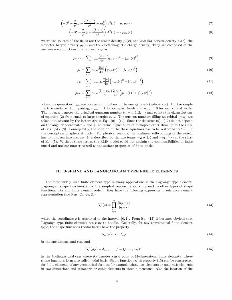
where the quantities nκ,n are occupation numbers of the energy levels (indices κ,n). For the simpleHartree model without pairing, nκ,n = 1 for occupied levels and nκ,n = 0 for unoccupied levels.The index n denotes the principal quantum number (n = 0, 1, 2, ...) and counts the eigensolutionsof equation (2) from small to large energies εκ,n. The nucleon numbers filling an orbital (κ, n) aretaken into account by the factors 2|κ| in Eqs. (9) - (12). Since the densities (9) - (12) do not dependon the angular coordinates θ and φ, no terms higher than of monopole order show up at the r.h.s.of Eqs. (5) - (8). Consequently, the solution of the these equations has to be restricted to l = 0 inthe description of spherical nuclei. For physical reasons, the nonlinear self-coupling of the σ-fieldhas to be taken into account. It is described by the two terms −g2 σ
2(r) and −g3 σ3(r) at the r.h.s.
of Eq. (5). Without these terms, the RMF-model could not explain the compressibilities in finitenuclei and nuclear matter as well as the surface properties of finite nuclei.
III. B-SPLINE AND LANGRANGIAN TYPE FINITE ELEMENTS
The most widely used finite element type in many applications is the Lagrange type element.Lagrangian shape functions allow the simplest representation compared to other types of shapefunctions. For any finite element order n they have the following expression in reference elementrepresentation (see Figs. 2a, 2c, 2e)
Nnq (ρ) =
n∏
l=0
l 6=q
(nρ− l)
(q − l)(13)
where the coordinate ρ is restricted to the interval[
0, 1]
. From Eq. (13) it becomes obvious thatLagrange type finite elements are easy to handle. Generally, for any conventional finite elementtype, the shape functions (nodal basis) have the property
Nnq (q
′/n) = δqq′ (14)
in the one dimensional case and
Nnq (~ρq′) = δqq′ , ~ρ = (ρ1, ..., ρM )T (15)
in the M-dimensional case where ~ρq′ denotes a grid point of M-dimensional finite elements. Theseshape functions form a so called nodal basis. Shape functions with property (15) can be constructedfor finite elements of any geometrical form as for example triangular elements or quadratic elementsin two dimensions and tetraedric or cubic elements in three dimensions. Also the location of the
4

mesh points which belong to a finite element can be distributed in almost arbitrary manner over thedomain of the element. In most cases, however, M-cube elements (intervals, squares, cubes, etc.)with a uniform distribution of the nodes are sufficient and allow extremely efficient calculations ofthe stiffness matrices for a given boundary value problem. The shape functions of such elements arerepresented as products of Lagrange polynomials (13)
N(q1 ,...,qM )
(q1,...,qM )(ρ1, ..., ρM ) =
M∏
i=1
Nniqi (ρi), qi, ..., ni, (16)
where ni denotes the order of the element in the direction of dimension i and (q) = (q1, ..., qM )forms the index tuple of the nodes.
The construction (16) of Lagrange type M-cube shape functions shows that 1-dimensional La-grange type finite elements allow the most simple generalization to M-cube meshes. A great advan-tage of such shape functions can also be seen from a technical view point. Implementations of thegeneral M-dimensional case in object oriented programming styles become simple. The amount ofdata required by an object which represents a Lagrangian M-cube finite element as reference elementis almost the same as in the 1-dimensional case if the orders n1, ..., nM are equal. In this specialcase the data representing all shape functions of a M-cube element comprise 2 ·ni ·n
Gi floating point
numbers where I denote by nGi the number of Gauss points on a Gaussian mesh in dimension i. In
the more general case where ni 6= nj for i 6= j and nGi 6= nG
j for i 6= j the amount of float pointnumbers required to represent all shape functions is
2
M∑
i=1
ni nGi (17)
which is still small compared to the number of values
2
M∏
i=1
ni nGi (18)
required for shape functions of arbitrary type and arbitrary distribution of the nodes over theelement.
The numerical cost for the integration of matrix elements reduces dramatically in cases whereoperators split up into products of operators each depending on a complementary subset of thecoordinates ρ1, ..., ρM . In the most ideal case an operator factorizes completely leading with Eq.(16) to a complete factorization of matrix elements.
⟨
N(n1 ,...,nM )
(q1 ,...,qM ) (ρ1, ..., ρM )
∣
∣
∣
M∏
i=1
Oi(ρi)
∣
∣
∣N
(n1,...,nM )
(q′1,...,q′
M)(ρ1, ..., ρM )
⟩
=
M∏
i=1
⟨
Nniqi (ρi)
∣
∣
∣Oi(ρi)
∣
∣
∣Nni
q′i(ρi)⟩
. (19)
This becomes obvious when I rewrite Eq. (17) in terms of a numerical Gauss integration
N∑
l1,...,lM
N(n)
(q)(ρl11 , ..., ρ
lMM )O(ρl11 , ..., ρ
lMM )N
(n)
(q)(ρl11 , ..., ρ
lMM )
M∏
i=1
wli =
M∏
i=1
N∑
li=1
Nniqi (ρ
lii )Oi(ρ
lii )N
ni
q′i(ρlii ) (20)
where, assuming that N is the number of Gauss points in each coordinate, the number of floatingpoint operations on the left hand side is greater than 4NM while on the r.h.s. it is smaller than3MN.
5

0 1 2 3 4 5 6index of mesh point
0.0
0.2
0.4
0.6
0.8
1.0
ampl
itude
of B
-spl
ine
1. ord.
2. ord.
3. ord.4. ord.
5. ord.
Fig. 1: B-spline functions of different orders increasing from 1 to 5.
These advantages of Lagrangian type finite elements gave us a reason to apply them in severalprevious studies and calculations (see references [13–15,9]). In these references, it has been shownthat Lagrangian finite elements provide an excellent tool for solving the equations of the RMFmodel in self-consistent iterations in coordinate space. In this manuscript, I present a new finiteelement technique using B-splines as shape functions and compare this method with the FEM basedon Lagrangian shape functions. B-splines have a compact support and are defined as polynomialspiecewise on intervals which are bounded by neighbored mesh points. The basic criterium in theconstruction of these basis functions is optimized smoothness over the whole support. This propertyis guaranteed if all derivatives up to the order n−1 obey the conditions of continuity in all matchingpoints of the mesh. The order n of a given B-spline corresponds to the degree of the polynomialsby which it is composed. In Fig. 1, examples are shown for B-splines of order one to five. n + 2mesh points are required to construct a B-spline of the order n. In contrast to Lagrangian shapefunctions, B-splines of any order do not change sign. A common property of both types of shapefunctions is expressed by
∑
p
Np(ρ) =∑
p
Bp(ρ) = 1 (21)
where p denotes the mesh point index. The fact, that B-splines of any order satisfy all theseconditions makes it impossible to find an expression in closed form in the sense of Eq. (13). Rather,they are generated by the following brief algorithm.
start: Bi,1(x) =
((xi+1 − xi))−1 xi ≤ x ≤ xi+1
0 x < xi, x > xi+1i = 0, ..., n;
Bi,k(x) =(x− xi)
(xi+k − xi)Bi,k−1(x) +
(xi+k − x)
(xi+k − xi)Bi+1,k−1(x) (22)
6
I define a B-spline finite element as a region which is bounded by two neighboring mesh points in theone-dimensional case or as a M-cube where the 2M corners are identical with the 2M mesh pointsof a cubic grid which are closest to the center of the cube. Obviously, this definition is restrictedto cubic grids but it will turn out to be extremely efficient in all cases where cubic finite elementdiscretizations can be applied.
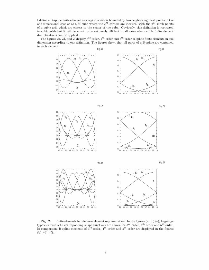
The figures 2b, 2d, and 2f display 3rd order, 4th order and 5th order B-spline finite elements in onedimension according to our definition. The figures show, that all parts of a B-spline are containedin each element.
0.0 0.1 0.2 0.3 0.4 0.5 0.6 0.7 0.8 0.9 1.0
-0.4
-0.2
0.0
0.2
0.4
0.6
0.8
1.0
Fig. 2a
(a)
N
N N
N0
1 2
3
0.0 0.1 0.2 0.3 0.4 0.5 0.6 0.7 0.8 0.9 1.00.0
0.1
0.2
0.3
0.4
0.5
0.6
0.7
B
BB
B0
12
3
(b)
Fig. 2b
0.0 0.1 0.2 0.3 0.4 0.5 0.6 0.7 0.8 0.9 1.0
-0.6
-0.4
-0.2
0.0
0.2
0.4
0.6
0.8
1.0
1.2
(c)
N
N
N
N
N0
1
2
3
4
Fig. 2c
0.0 0.1 0.2 0.3 0.4 0.5 0.6 0.7 0.8 0.9 1.00.0
0.1
0.2
0.3
0.4
0.5
0.6
B
B
B
B
B0
1
2
3
4
(d)
Fig. 2d
0.0 0.1 0.2 0.3 0.4 0.5 0.6 0.7 0.8 0.9 1.0-1.0
-0.8
-0.6
-0.4
-0.2
0.0
0.2
0.4
0.6
0.8
1.0
1.2
N
N N NN
N0
12 3
4
5
(e)
Fig. 2e
0.0 0.1 0.2 0.3 0.4 0.5 0.6 0.7 0.8 0.9 1.00.0
0.1
0.2
0.3
0.4
0.5B
B
B
B
B
B
(f)
0
1
2 3
4
Fig. 2f
5
Fig. 2: Finite elements in reference element representation. In the figures (a),(c),(e), Lagrangetype elements with corresponding shape functions are shown for 3rd order, 4th order and 5th order.In comparison, B-spline elements of 3rd order, 4th order and 5th order are displayed in the figures(b), (d), (f).
7

A B-spline of order n is determined by n + 2 mesh-points through the algorithm (22) and thesupport is composed by n+1 intervals. However, the pieces which are contained in a single elementbelong to different B-splines each located at another mesh point and determined by a different setof mesh points. They are the overlap sections of all splines which are not zero in the consideredelement. This fact has to be taken into account especially if nonuniform meshes are used. As aconsequence, the amplitudes of the shape functions in such a finite element depend on the positionof all mesh points which are in the support of all contributing B-splines. Most of these mesh pointsare outside of the element and belong to other elements. Therefore, the degree of ”interaction”between neighbored elements is maximized and much higher than for elements of Lagrange typewhere only next neighbor elements ”interact” through their outermost contact grid points. Thisleads to a strong reduction of the total number of required mesh points as I will demonstrate insection 5.
A disadvantage, however, appears when non-uniform meshes are used. As it has been discussedin reference [14], Lagrangian elements can be mapped on a reference element through linear affinetransformations. This is even possible for non-uniform meshes. Therefore, Lagrangian shape func-tions need to be evaluated only once in the reference element and amplitudes and abscissas canbe accessed by means of a pointer to that reference element. These advantages are also valid forB-splines as long as uniform meshes are used. In the case of non-uniform meshes the algorithm(22) has to be evaluated for each argument taken on the global region. This leads to a reductionof storage requirement but increases the numerical cost by a factor which corresponds to the num-ber of floating point operations which are necessary to carry out the scheme (22). Consequently,the numerical effort in the calculation of the stiffness matrices of a given problem increases by thesame factor. On the other hand, the number of algebraic equations resulting from a finite elementdiscretization is usually large and the numerical cost to solve these equations increases faster withthe number of equations (∼ number of mesh points) than the numerical cost in the calculation ofthe stiffness matrices with the number of mesh points. This trend is even enhanced for increasingdimension M of the descretization where the condition of the stiffness matrices becomes worse.B-splines finite elements might therefore be superior in multidimensional FEM discretizations ascompared to Lagrangian finite elements.
IV. THE FEM DISCRETIZATION
A basic principle of FEM is the approximation of the solution for a given problem in a space ofshape functions which have compact support and existing continuous weak derivative of maximumdegree m. Together with a p-norm which is for all those functions defined as
‖ϕ‖m,p :=(
m∑
α=0
∫
Ω
|Dαϕ(x)|p)1/p
, (23)
the above given space is a Banach space. According to the norm it is usually called Sobolev spaceWm
p (Ω) where Ω may be any compact domain of the coordinate space. SinceWmp (Ω) is complete, the
solutions of any partial differential equation of an order not higher than m can be approximated toarbitrary precision in Wm
p (Ω) on the whole domain Ω. This property plays an important role for thesolution of differential equations with computational methods because finite element discretizationsof the domain Ω correspond to subsets of linear independent functions of Wm
p (Ω) and because therepresentation of functions of Wm
p (Ω) on the computer is simple. In FEM, Ω is subdivided intoa large number of small sub-domains which are called finite elements. Each element is support ofa certain number of shape functions which is equivalent to the number of constraints set on theelement. These functions span up a finite element space. The corners of the elements are located ona finite element mesh. However, additional mesh points can exist in the interior or on the surfaceof each element and additional constraints as derivatives of any order can be applied. In such casesthe order of the element is higher than first order.
In the following, I discuss the finite element discretization of the Eqs. (2) and Eqs (5) to (8) forboth types Lagrangian and B-spline elements. In the present application a nodal basis Np(r) isused in the case of Lagrange elements and a non-nodal basis Bp(r) is used in the case of B-splineelements. Examples for discretizations with elements of 3rd order are displayed for both types in Fig.3a and 3b. Each Lagrangian element in Fig. 3a has two boundary nodes and two additional nodesin the interior whereas the B-spline elements in Fig. 3b are free of interior nodes. In the B-spline
8

method additional nodes are required outside of the region of integration in order to generate theshape functions which have non-zero overlap with the inner region. I use the notation Np(ρ) andBp(ρ) (0 ≤ q ≤ n) for shape functions in reference element representation, and Np(r) or Bp(r)(1 ≤ p ≤ nnod) for shape functions Np and Bp on the global mesh in the r-coordinate space. Usingthe standard representation for the Pauli matrices, the Dirac equation (2) is written in matrix form
[
(∂r + r−1) · σ3σ1 − κr−1 · σ1 + (m+ S(r)) · σ3 + V (r) · 12
]
Φ(r) = ε12 Φ(r). (24)
0 1 2 3 4 5 6 7 8 9 10r [fm]
-8
-7
-6
-5
-4
-3
-2
-1
0
1
2
(a)
Fig. 3a
0 1 2 3 4 5 6 7 8 9 10 11 12 13r [fm]
-8
-7
-6
-5
-4
-3
-2
-1
0
1
2
3
Fig. 3b
(b)
Fig. 3: Global discretizations with 3rd order finite elements (a) of Lagrangian type and (b)of B-spline type. In both examples a total number of 16 mesh points is used in the region betweenr = 0 fm and r = 10 fm.
For the nucleon spinor I use the FEM ansatz
Φ(r) =∑
p
upBp(r) (25)
with B-spline functions Bp(r) and node variables up := (u(g)p , up(f))
T . In a Lagrangian FEMansatz, the shape functions Bp(r) defined in (25) are replaced by the shape functions Np(r). In theweak formulation of the eigenvalue problem (2), the weighted residual (see [14]) leads to algebraicequations of the form
∑
p
⟨
wp′(r)
∣
∣
∣
[
(∂r + r−1) · σ3σ1 − κr−1 · σ1 + (m+ S(r)) · σ3 + V (r) · 12
]∣
∣
∣Bp(r)
⟩
up =
ε⟨
wp′(r)∣
∣
∣12
∣
∣
∣Bp(r)
⟩
up (26)
with weighting functions wp′(r). The weighting functions are chosen
wp′(r) =(
1−(
r
rmax
)2)
r2 rlg/f Bp(r) (27)
in the case of B-spline elements or
wp′(r) =(
1−(
r
rmax
)2)
r2 rlg/f Np(r) (28)
when Lagrangian shape functions are used in ansatz (25).
lg =
−κ− 1 κ < 0;κ κ > 0;
(29)
9
lf =
−κ κ < 0;κ− 1 κ > 0;
(30)
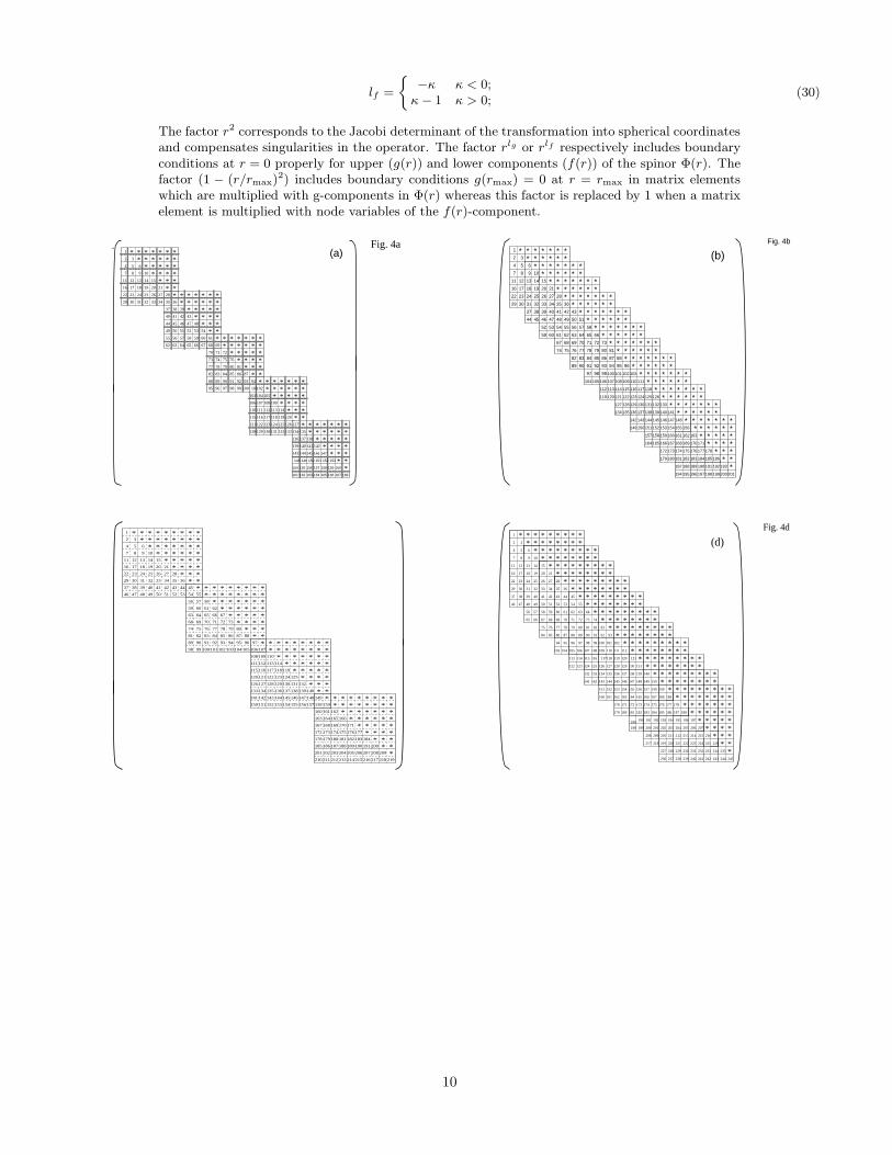
The factor r2 corresponds to the Jacobi determinant of the transformation into spherical coordinatesand compensates singularities in the operator. The factor rlg or rlf respectively includes boundaryconditions at r = 0 properly for upper (g(r)) and lower components (f(r)) of the spinor Φ(r). Thefactor (1 − (r/rmax)
2) includes boundary conditions g(rmax) = 0 at r = rmax in matrix elementswhich are multiplied with g-components in Φ(r) whereas this factor is replaced by 1 when a matrixelement is multiplied with node variables of the f(r)-component.
********
*
*****************
*****
***
***
* * * * * ** * * * * *
* * * * ** * *
* ** *
* * * * * ** * * * *
* * * ** *
****
*
* ***
**
**
*
***
*
* ***
* ** ***
* *
*
**
**
*
1
2 3
4 5 6
7 8 9 10
11 12 13 14 15
16 17 18 19 20 21
22 23 24 25 26 27 28
29 30 31 32 33 34 35 36
37 38 39
40 41 42 43
44 45 46 47 48
49 50 51 52 53 54
55 56 57 58 59 60 61
62 63 64 65 66 67 68 69
70 71 72
73 74 75 76
77 78 79 80 81
82 83 84 85 86 87
88 89 90 91 92 93 94
95 96 97 98 99 100 102101
103 104 105
106 107 108 109
110 112 113 114
115 117 118 119 120
121 122 123 124 125 126 127
128 129 130 131 132 133 134 135
136 137 138
139 140 141 142
143 144 145
* * * * * * ** * * * * *
*****
**
146 147
148 149 150 151 152 153
154 155 156 157 158 159 160
161 162 163 164 165 166 167 168
116
111
Fig. 4a(a)
**
1
10
11 12 13 14
16 17 18 19 20 21
22 23 24 26 27 28
29 30 31 32 33 35 36
37 38 39 40 41
44 45 46 47 48 49 50 51
52 53 54 55 56 57 58
59 60 61 62 63 64 65 66
67 68 69 70 71 72 73
74 75 76 77 78 79 80 81
82 84 85 86 87 88
89 90 91 92 93 94 95
2 3
654
987
15
25
34
42 43
97
83
98 99 100 101 102
104 105 106 107 108 109 110
112
120 121 122 123 124 125
127 128 129 130 131 132 133
134 135 136 137 138 139 140 141
142 143 144 145 146 147 148
149 150 151 152 153 154 155 156
157 158 159 160 161 162 163
164 165 166 167 168 170
172 173 174 175 176 177
171169
179 180 181 182 183 184 185 186
187 188 189 190 191 192 193
194 195 196 197 198 199 200 201
126
111
96
118117116114113
119
178
103
115
Fig. 4b* * * * * * *
* * * * * ** * * * * * *
* * * * * ** * * * * * *
* * * * * ** * * * * * *
* * * * *** * * * * * *
* * * * ** * *
** * * *
* * * * ** * * * * * *
* * * * * ** * * * * * *
* * * * * ** * * * * * *
* * * * * ** * * * * * *
* * * * * ** * * * * * *
* * * * * ** * * * * * *
* * * * * ** * * * *
* * * ** * *
* **
*
(b)
1 * * * * * * *
* * * * * * ** * * * ** * * *
* * ** * *
* ** * * * *
**
*
* * * ** * * * * * * *
* * * * * * ** * * * * *
* * * * ** * * *
* *** * * * * * * * *
* * * * * * *
**
** * * * * * *
* * * * * ** * * * *
* * * ** * *
* ** * * * * * * *
* * * * * *** * * * * *
* * * * ** * * *
* * ** *
*
2 3
4 5 6
7 8 9 10
11 12 13 14 15
16 17 18 19 20 21
22 23 24 25 26 27 28
29 30 31 32 33 34 35 36
37 38 39 40 41 42 43 44 45
46 47 48 49 50 51 52 53 54 55
56 57 58
59 60 61 62
63 64 65 66 67
68 69 70 71 72 73
74 75 76 77 78 79 80
81 82 83 84 85 86 87 88
89 90 91 92 93 94 95 96 97
98 99 100 101 102 103 104 105 106 107
108 109 110
111 112 113 114
115 116 117 118 119
120 121 122 123 124 125
126 127 128 129 130 131 132
133 134 135 136 137 138 139 140
141 142 143 144 145 146 147 148 149
150 151 152 153 154 155 156 157 158 159
160 161 162
163 164 165 166
167 168 169 170 171
172 173 174 175 176 177
178 179 180 181 182 183 184
185 186 187 188 189 190 191 200
202201 205 206204203 207 208 209
210 211 212 213 214 215 216 217 218 219*
********
** * * * * * * *
* 1
2
4 6
7 9 10
11 12 13 14 15
16 17 18 19 20 21
22 23 26 28
29 30 31 32 33 34 35 36
38 39 40 41 42 43 4437 45
46 47 48 49 50 51 52 53 54 55
3
5
8
24 25 27
56 57 58 59 60 61 62 63 64
65 66 67 68 69 70 71 72 73 74
7675 78 80 81 82 83
84 85 86 87 88 89 90 91 92 93
77 79
94 95 96 97 98 99 101100 102
103 104 105 106 107 108 109 110 111 112
113 114 115 116 117118 119 120 121
122 123 124 125 126 127 128 129 130 131
132 133 134 135 136 137 138 139 140
141 142 143 144 145 146 147 148 149 150
151 152 153 154 155 156 157 158 159
160 161 162 163 164 165 166 167 168 169
170 171 172 173 174 175 176 177 178
179 180 181 182 183 184 185 186 187 188
189 190 191 192 193 194 195 196 197
198 199 200 201 202 203 204 205 206 207
208 209 210 211 212 213 214 215 216
217 218 219 220 221 222 223 224 225 226
227 228 229 230 231 232 233 234 235
236 237 238 239 240 241 242 243 244 245
*********
*********
******
******** *
*
**********
*******
**********
*******
**********
*******
**********
*******
**********
*******
**********
*
*****
*
*** *
*** *
*** *
*** *
*
*********
*********
***
*** *
****
***
**
*** *
*** *
*** *
*
*****
*****
**
***
Fig. 4d
(d)
10

1 * * * * * * *
* * * * * ** * * ** * ** *
* ** *
*
*
*
* * * * * * ** * * * * *
* * * * ** * * *
* *** * * * *
* * *
**
** * *
* ** * * * *
* * * ** * *
* ** * * * * * *
* * * * *** * * * *
* * * ** * *
* **
(e)2 3
4 5 6
7 8 9 10
11 12 13 14 15
16 17 18 19 20 21
22 23 24 25 26 27 28
29 30 31 32 33 34 35 36
37 38 39 40 41 42 43 44 45
46 47 48 49 50 51 52 53 54 55
56 57 58 59 60 61 62 63 64 65 66
67 68 69 70 71 72 73 74 75 76 77 78
*** * * * * * * * * *
*** *
*** *
*** *
*** *
**
***
*
******
******
******
******
****
****
****
****
****
****
79 80 81
8382 84 85
86 87 88 89 90
91 92 93 94 95 96
97 98 99 100 101 103102
105104 106 107 108 109 110 111
112 113 114 115 117118119120116
121 122 123 124 125 126 127 128 129 130
131 132 133 134 135 136 137 138 139 140 141
142 143 144 145 146 147 148 149 150 151 152 153
154 155 156
157 158 159 160
161 162 163 164 165
166 167 168 169 170 171
172 173 174 175 176 177 178
179 180 181 182 183 184 185 186
187 188 189 190 191 192 193 194 195
196 197 198 199 200 201 202 203 204 205
206 207 208 209 210 211 212 213 214 215 216
217 218 219 220 221 222 223 224 225 226 227 228
Fig. 4e1
2
4
7 10
11 12 13 14 15
16 17 18 19 20 21
22 23 24 25 26 27
90
88878685848382818079
787776757473727170696867
6665646362616059585756
55545352515049484746
454443424140393837
3635343332313029
28
3
5
8
6
9
89
* * * * * * * * * * ** * * * * * * * * *
* * * * * * * * * * ** * * * * * * * * *
* * * * * * * * * * ** * * * * * * * * *
* * * * * * * * * * ** * * * * * * * * *
* * * * * * * * * * ** * * * * * * * * *
* * * * * * * * * *** * * * * *
92 93 94 95 96 97 9891 99 100 101
102 103 104 105 106 107 108 109 110 111 112
113 114 115 116 117 118 119 120 121 122 123 124
125 126 127 128 129 130 131 132 133 134 135
136 137 138 139 140 141 142 143 144 145 146 147
148 149 150 151 152 153 154 155 156 157 158
159 160 161 162 163 164 165 166 167 168 169 170
171 172 173 174 175 176 177 178 179 180 181
182 183 184 185 186 187 188 189 190 191 192 193
194 195 196 197 198 199 200 201 202 203 204
205 206 207 208 209 210 211 212 213 214 215 216
117 118 119 120 121 122 123 124 125 126 127
128 129 130 131 132 133 134 135 136 137 138 139
140 141 142 143 144 145 146 147 148 149 150
151 152 153 154 155 156 158 159 160 161 162 163
* * *** * * * ** ** * * * *
* * * ** * * ** * * * * *
************ * * * * * * * * *
* * * * * * * * * * ** * * * * * * * * *
* * * * * * * * ** * * * * * * * *
*** * * * * * * * * * *
* * * * * * * * * ** * * * * * * * *
* * * * * * * ** * * * * * *
* * * * * ** * * * *
* * * *
**
Fig. 4f(f)
164 165 167 168 169 170 171 172 173 174 * * ** *
*
175
176 177 178 179 180 181 182 183 184 185 186 187
188 189 190 191 192 193 194 195 196 197 198
199 200 201 202 203 204 205 206 207 208 209 210
Fig. 4: Occupation patterns of stiffness matrices which result from the finite element dis-cretization of Eq. (2). The figures (a), (c), (e) display matrices which correspond to 3rd order, 4th
order and 5th order Lagrange type FEM. Figues (b), (d), (f) display patterns which result from 3rd
order, 4th order and 5th order B-spline FEM discretizations. The numbers represent counter indicesused in a vector storage technique.
The boundary conditions at r = 0 fm depend on the quantum number κ and are defined in thefollowing way.
f(r = 0) = 0 for κ = −1 (31)
g(r = 0) = 0 for κ = +1 (32)
g(r = 0) = 0 and f(r = 0) = 0 for |κ| > 1. (33)
The system of algebraic equations (26) forms a generalized eigenvalue problem of the form Au =εN u with stiffness matrices A and N can be analyzed from the resulting matrix equation
[
S1 ⊗ σ3σ1 + S2 ⊗ σ3σ1 − κS2 ⊗ σ1 +mS3 ⊗ σ3 + S4 ⊗ σ3 + S5 ⊗ 12
]
u = ε[
S3 ⊗ 12
]
u (34)
where u is a vector with components (u(g)1 , u
(f)1 , ..., u
(g)n , u
(f)n )T . The symbols S1 to S5 denote the
stiffness matrices of the operators on the l.h.s. of Eq. (24),
S1 =⟨
wp′(r)
∣
∣
∣∂r
∣
∣
∣Bp(r)
⟩
,
S2 =⟨
wp′(r)∣
∣
∣r−1∣
∣
∣Bp(r)
⟩
,
S3 =⟨
wp′(r)∣
∣
∣Bp(r)
⟩
,
S4 =⟨
wp′(r)
∣
∣
∣S(r)
∣
∣
∣Bp(r)
⟩
,
S5 =⟨
wp′(r)
∣
∣
∣V (r)
∣
∣
∣Bp(r)
⟩
. (35)
In Figs. 4a-f, occupation patterns of the stiffness matrices A are displayed for Lagrangian and B-spline finite element discretizations. The matrices in Figs. 4a, 4c, 4e result from the Lagrange FEMwith 3rd order, 4th order and 5th order finite elements. For comparison, I show the correspondingstiffness matrices of the B-spline FEM in Figs. 4b, 4d, 4f. The sub-block structure of 2×2-blocks inall matrices results from the fact that Eq. (2) is a system of two coupled equations. The number ofoccupied 2× 2-blocks for a given order nord in the Lagrange FEM is nfe ·
[
(nord)2 +2n]
+1 while in
the B-spline method the occupation increases to nfe ·[
2(nord)2 + n]
+ 1. nfe denotes here for bothcases the number of finite elements used in the Lagrange method and is different from the numberof elements which is used in the B-spline FEM.
11

The FEM discretization of the Klein-Gordon equations (5) to (8) is described in the appendix.Finally, the coupled system of differential equations (2), (5) to (8) is replaced by a system of linearalgebraic equations
A(~σ, ~ω 0, ~ρ 0, ~A 0)u = εN u (36)
for the node variables u(g)p , u
(f)p of nucleon spinors, and
Bσ(~σold)~σ = ~r(s) (37)
Bω ~ω0 = ~r(v) (38)
Bρ ~ρ0 = ~r(3) (39)
BA~A 0 = ~r(em) (40)
for the node variables σp, ωp, ρp, and Ap of the meson fields σ(r), ω0(r), ρ0(r), and photon fieldA0(r). The occupation patterns of the matrices Bσ, Bω, Bρ, and BA0 for various shape functionsare very similar to those of the matrix A (Figs. 4a-d). The main difference is that 2× 2-blocks haveto be replaced by single matrix elements.
V. ANALYSIS OF SPURIOUSITY
The appearance of spurious solutions in applications of FEM is a well known problem in general.First applications of the finite element method in relativistic nuclear physics [13] have shown thatspurious solutions appear in the spectra of the Dirac equation. Linear finite elements have beenused to calculate solutions of the relativistic nuclear slab model. Comparisons of the solutions withsolutions that have been obtained with other numerical techniques (shooting method) have shownthat FEM reproduces the physical spectra very well and that spurious solutions have no influence. Ina further step [14] Lagrangian finite elements of 1. to 4th order have been used in the self-consistentsolution of the RMF equations of sperical nuclei. In these calculations, it has been shown (up to4th order) that the density of spurious solutions in the spectra decreases for increasing order of theelements.
In this sections, I present a systematic study of the spurious spectra which appear in the sphericalsymmetric case. In the initial step of a self-consistent ground state calculation of 208
82 Pb, Woods-Saxon potentials
S(r) = S(0)(
1 + exp(r − rsa
)))
−1
, (41)
V (r) = V (0)(
1 + exp(r − rsa
))
−1
, (42)
are used for the scalar potential S(r) and for the vector potential V (r). For 208Pb the valuesof these potentials at r = 0 fm are chosen S(0) = −395MeV and V (0) = 320MeV, respectively.a = 0.5 fm and rs = 9.0 fm. The calculation is performed on a uniform radial mesh extendingfrom rmin = 0 fm to rmax = 20 fm. A smaller value rmax = 12 fm would be sufficient for 208Pbto obtain good approximations of the bound single particle states. For a good resolution of thecontinuum, however, a large extension of the mesh in coordinate space is necessary. An extremelyhigh number of 200 mesh points has been used in the calculation of the sprectra shown in Fig. 5ato Fig. 5f. The reason for that choice will become clear from the subsequent discussion of Fig.6. For a nucleon mass of 939MeV (parameter set NL3), the Dirac gap extends from −939MeVto +939MeV. Bound solutions are expected to have energies which are located in the Dirac gap.In the following calculations an energy window ranging from −1300MeV to +1300MeV has beenchosen which covers parts of the lower and upper continuum as well.
The results which are presented in the subsequent discussion correspond to the first iteration stepand a value κ = −1 (s-waves). Spurious spectra of similar eigenvalue distributions are obtained forall other κ-values (κ = +1,±2,±3, ...). Disregarding the fact that the eigensolutions change whilethey converge, very similar results are found in all iteration steps of the selfconsistent iteration.
One of the most interesting questions to be answered in the present paper is, whether the ap-pearance of spurious solutions can be avoided using B-spline finite elements instead of Lagrangianelements. Since both methods are identical in the case of 1st order, spurious solutions appear also
12

in the B-spline FEM. However, from that one can not conclude that spurious solutions appear inFEM discretizations with B-splines of higher order. The following six figures Fig. 5a to Fig. 5fdisplay energy spectra of Eq. (2) which have been calculated for many different orders with bothmethods, the Lagrange FEM and the B-spline FEM. In Fig. 5a and Fig. 5b the positive and neg-ative spectra are shown for 1st order to 4th order finite elements. The white circles correspond tophysical eigenvalues which have been calculated with Lagrange type elements. They are located atthe same energies as the white triangles which correspond to physical eigenvalues obtained with theB-spline FEM. The figures show that the physical spectra are independent on the order and on theused method. However, the number of black filled circles and filled triangles in the spectra decreasesfor increasing order of the used shape functions. The filled symbols indicate eigenvalues of spurioussolutions. It turns out that the distributions of spurious eigenvalues over the entire energy rangeare identical for both methods and in all orders. In comparison to the Lagrange FEM, the B-splinemethod does obviously not reduce the number of spurious states as long as the order is the sameused in both methods. However, for both methods, the density of spurious solutions in the spectracan be strongly reduced by increasing the order of the finite elements. Particularly, from Fig. 5cto Fig. 5f, on can see, that the spurious eigenvalues drift away from the Dirac gap when the orderis increased. Consequently, for any energy window there exists an order which is high enough sothat no spurious solutions appear in the window. An exception forms the region between the lowestpositive physical eigenvalue and the highest negative physical eigenvalue. For all element orderswith both methods, no spurious solution has been found in that region.
50 70 90 110 130 150 170 190 210index
800
850
900
950
1000
1050
1100
1150
1200
1250
1300
tota
l en
erg
y [M
eV
]
(a)
Fig. 5 a
1. ord. 2. ord. 3. ord. 4. ord.
0 20 40 60 80 100 120 140 160 180index
-1300
-1200
-1100
-1000
-900
-800
-700
-600
-500
-400
-300
-200
-100
tota
l en
erg
y [M
eV
]
1. ord. 2. ord. 3. ord. 4. ord.(b)
Fig. 9 b
40 60 80 100 120 140 160 180 200index
800
900
1000
1100
1200
1300
tota
l en
erg
y [M
eV
]
(c)
Fig. 5 c
5. ord. 6. ord. 7. ord. 8. ord.
0 20 40 60 80 100 120 140 160 180index
-1300
-1200
-1100
-1000
-900
-800
-700
-600
-500
-400
-300
-200
-100
tota
l en
erg
y [M
eV
]
(d)
Fig. 5 d
5. ord. 6. ord. 7. ord. 8. ord.
13

40 60 80 100 120 140 160 180 200index
800
900
1000
1100
1200
1300
tota
l en
erg
y [M
eV
]
9. ord. 10. ord. 11. ord. 12. ord.
Fig. 5 e
0 20 40 60 80 100 120 140 160 180index
-1300
-1200
-1100
-1000
-900
-800
-700
-600
-500
-400
-300
-200
-100
tota
l en
erg
y [M
eV
]
9. ord. 10. ord. 11. ord. 12. ord.
Fig. 5 f
Fig. 5: Energy eigenvalues of the Dirac equation (2) for the case κ = −1. The spectraare compared for the Lagrange FEM (circles) and the B-spline FEM (triangles). The used finiteelement orders are indicated in the figures. Filled symbols correspond to spurious eigenvalues. Alleigenvalues which appear in the energy window
[
−1300MeV, +1300MeV]
are displayed for 1st order
to 12th order elements.
It is also important to analyze the dependence of the spurious spectrum on the number of meshpoints. In Fig. 6, the number of spurious solutions is displayed for different orders as a function ofthe number of mesh points in a constant radial box (rmin = 0 fm, rmax = 20 fm). The results showthat the number of spurious solutions is independent on the number of mesh points if this numberis sufficiently large. This is true for all orders of finite elements. The solid lines in Fig. 6 showthe results which have been obtained for the above defined Woods-Saxon potentials. For all finiteelement orders the number of spurious states in the above defined energy window increases at lowmesh point numbers and decreases monotonically at high mesh point numbers. At large numbersof mesh points (”asymptotic region”) the number of spurious solutions is constant for all elementorders. This has been tested up to the very large number of 600 mesh points but is not shown inthe figure. For the calculation of the spectra shown in Fig. 5a to 5b, I have used a number of meshpoints (200) which is in that asymptotic region to make sure that they (in particular the spuriousspectra) are independent on the number of mesh points.
An explanation for the curves in Fig. 6 is found with the concept of Sobolev space. In reference[14] it has been outlined that a Sobolev space Wm
p (Ω) is a completion of the test function spaceC∞
0 (Ω) with respect to the Sobolev norm ‖ · ‖m,p defined in Eq. (23). Thus, C∞
0 (Ω) ⊂ Wmp (Ω) for
all integer numbers m ≥ 0. All spaces Wmp (Ω), where m > 0, are subspace of the largest Sobolev
space W 0p (Ω) and
Wm+1p (Ω) ⊂Wm
p (Ω) for all m ≥ 0. (43)
The shape functions of mth order finite elements are element of Wmp (Ω) but the shape functions of
any lower order finite elements are not in Wmp (Ω). In finite element discretizations of low order m
is small and one works in a correspondingly large space Wmp (Ω). The weak form, of a differential
equation, expressed in terms of the weighted residual, allows more solutions than the solutions ofthe original problem. All solutions which are found for a certain FEM order m are element ofWm
p (Ω). For increasing order m the space Wmp (Ω) shrinks and the number of spurious solutions in
the weak form is reduced while all physical solutions are maintained. This is seen from Fig. 5a toFig. 5f for one large number of mesh points. It explains in general the reduction of the numberof unphysical solutions in Fig. 6 for all mesh point numbers when the order of the FEM-ansatz isincreased. For a uniform finite element mesh with constant width h, the mth order shape functionsof the whole FEM discretization span up a space Sm
h (Ω). Starting from an initial discretizationwhere h0 is large, a sequence of spaces Sm
hi(Ω) i = 0, 1, 2, ... is generated when the mesh is refined for
increasing index i, where hi+1 < hi. The direct sum of the spaces Smhi(Ω) converges against Wm
p (Ω)
and thus∞⊕
i=0
Smhi(Ω) =Wm
p (Ω). Different spaces Smhi(Ω) and Sm
hj(Ω) where i 6= j can have non-trivial
intersection. There are even cases where Smhi(Ω) ⊂ Sm
hj(Ω) when hi < hj . In the example of the
two spaces S1h(Ω) and S1
h/2(Ω) it is obvious that S1h(Ω) ⊂ S1
h/2(Ω) since each linear shape function
14

which is basis function in S1h(Ω) can be represented as linear combination of shape functions (basis
functions) of S1h/2(Ω). The strong increase of the graphs in Fig. 6 at small mesh point numbers,
where h is large, is explained by the fact that the spaces Smh (Ω) become large for decreasing h. The
number of spurious solutions which appear in Smh (Ω) increases simultaneously. However, there is a
second effect which is superposed to this first one.
50 100 150 200 250 300number of mesh points
1
3
5
7
9
11
13
15
17
19
21
23
25
27
num
ber
of s
purio
us s
olut
ions
1. ord.
1. ord.
2. ord.
2. ord.
3. ord.
3. ord.
6. ord.
4. ord.
5. ord.
Fig. 6: Dependencies of the number of spurious solutions on the number of mesh pointsare shown for 1st order to 6th order finite elements. A constant mesh size ranging from 0 fm to20 fm has been used in the calculations. The solid (and dot-dashed) lines show results obtainedfor Woods-Saxon potentials V (r) and S(r). The dashed lines show corresponding results for zeropotential.
Spurious solutions which have a very high number of oscillations can only be completely resolved inspaces Sm
h (Ω) where h is small. However, spurious states with high frequency can appear in subspacesSmh(Ω) where h = ν ·h (ν = 1, 2, 3, ...) and where only a fraction of the oscillations is resolved. Since
the corresponding kinetic energy which contributes to the total energy is small, these solutionsappear in the above chosen energy window. If the number of mesh points is increased, additionaloscillations are resolved and the kinetic energy increases correspondingly. The corresponding totalenergy appears no longer in the energy window. In the negative energy range such solutions areshifted further into the negative continuum.
In Fig. 7a and Fig. 7b, spurious energy spectra are displayed for many different mesh pointnumbers. First order finite elements have been used. The mesh point numbers have been chosenaround the maximum of the solid curve in Fig. 6 which corresponds to first order. The solid linesconnect spurious eigenvalues which appear at constant mesh point number which is indicated bythe numbers atop of each line.
15

50 70 90 110 130 150 170 190 210 230 250index
800
900
1000
1100
1200
1300to
tal e
nerg
y [M
eV
]
Dirac gap
15
01
45
14
01
35
13
01
25
12
01
15
11
01
05
10
09
59
08
58
075
70
65
60
59
58
57
56
55
54
53
52
51
50
Fig. 7a
(a)
0 10 20 30 40 50 60 70 80 90 100index
-1300
-1200
-1100
-1000
-900
-800
-700
-600
-500
-400
-300
-200
-100
tota
l energ
y [M
eV
]
Dirac
gap
70
75
80 85
90 95
10
0
10
5
11
01
15
12
01
25
13
01
35
14
0
14
51
50
Fig. 7b
(b)
Fig. 7: Spurious spectra of the first order finite element discretization are displayed for differentmesh point numbers. The solid lines connect eigenvalues which belong to the same discretization.The number of mesh points is indicated above each line.
VI. NUMERICAL PRECISION
In the following, I present an analyse of the numerical precision of both methods and compare theresults. The quality in the approximation of the exact solutions of (23) depends essentially of theorder of the FEM-ansatz and on the number of mesh points used in a given domain Ω =
[
rmin, rmax
]
.In the subsequent tables, neutron single particle eigenvalues are listed systematically for increasingnumber of mesh points and increasing order of used finite elements. The eigenvalues correspondto solutions which have been obtained in the initial step of a selfconsistent calculation for 40Ca.In the first iteration step, Woods-Saxon potentials of the form (41) and (42) have been used withparameters S(0) = −395MeV, V (0) = 320MeV, a = 0.5 fm and rs = 6.0 fm. The mesh size has beenkept fixed with boundaries at rmin = 0 fm and rmax = 10 fm. In Table 1a neutron single particleenergies which have been calculated with linear finite elements are shown for the initial Woods-Saxon potential. For increasing number of mesh points (see left column), the number of unchangeddecimal places reaches 8 at 200 mesh points. A comparison with the last row of Table 1b showsthat for linear elements the last digit (decimal place 10) has not stabilized at the extremely largemesh point number 600. Table 1b displays results that have been calculated with finite elements of3rd order. Between 109 and 121 mesh points (36-40 elements), the results have stabilized in all 10digits. In Table 1c, I show the corresponding results which have been obtained with finite elementsof 4th order. To demonstrate the enormous improvement in the precision, the results are displayedup to 12 digits. Between 81 and 93 mesh points the 8th digit becomes stable and between 125 and145 mesh points the precision achieves 12 digits.
1. Order
nnod E1s1/2 E1p3/2 E1p1/2 E1d5/2 E2s1/2 E1d3/2
10 65.88844974 57.33594611 56.42536540 47.45864481 42.33620819 45.3452093820 65.88133752 57.31827220 56.39907816 47.42408909 42.19281200 45.2898114130 65.88108502 57.31763456 56.39825020 47.42279518 42.18737854 45.2880424440 65.88104432 57.31753150 56.39811692 47.42258515 42.18648990 45.2877564550 65.88103335 57.31750369 56.39808101 47.42252842 42.18624969 45.2876792760 65.88102944 57.31749377 56.39806819 47.42250815 42.18616380 45.2876517170 65.88102777 57.31748952 56.39806272 47.42249948 42.18612708 45.2876399380 65.88102696 57.31748747 56.39806006 47.42249529 42.18610928 45.2876342290 65.88102653 57.31748638 56.39805866 47.42249306 42.18609982 45.28763119
16
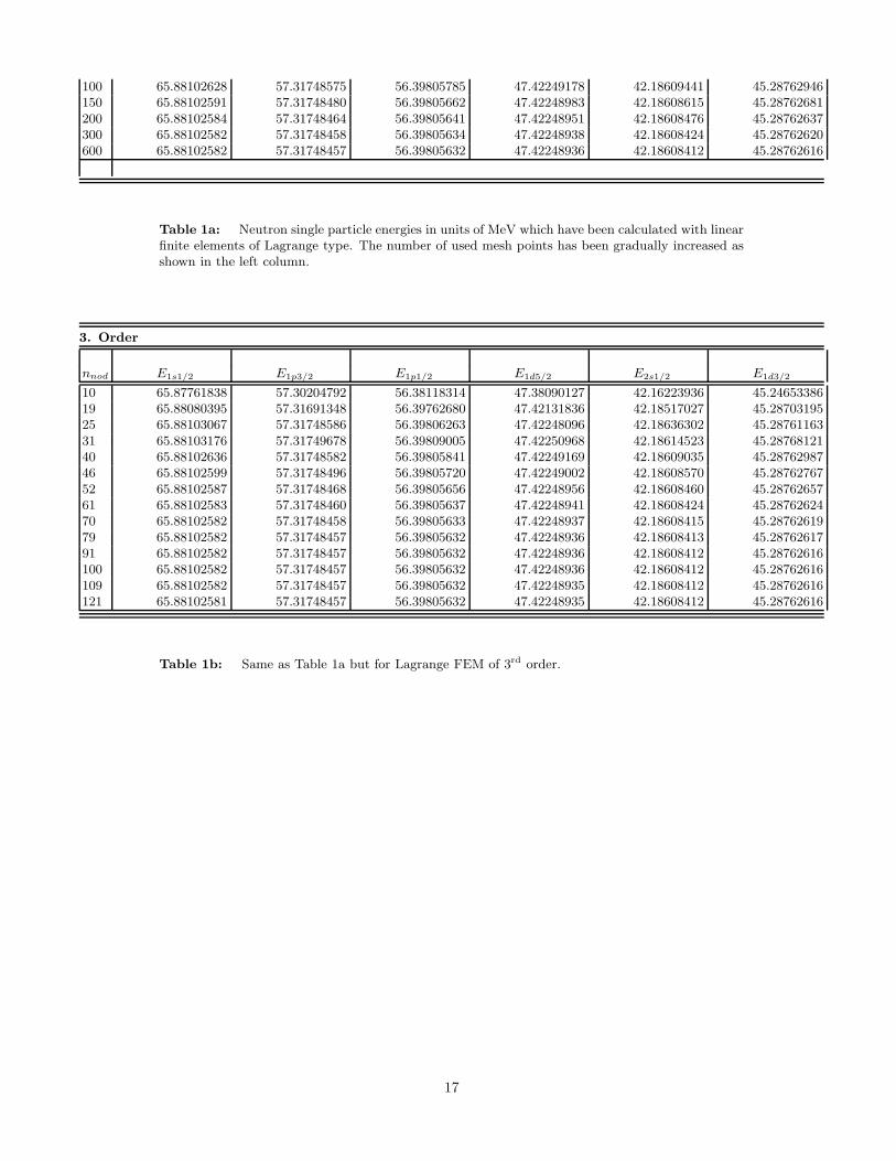
100 65.88102628 57.31748575 56.39805785 47.42249178 42.18609441 45.28762946150 65.88102591 57.31748480 56.39805662 47.42248983 42.18608615 45.28762681200 65.88102584 57.31748464 56.39805641 47.42248951 42.18608476 45.28762637300 65.88102582 57.31748458 56.39805634 47.42248938 42.18608424 45.28762620600 65.88102582 57.31748457 56.39805632 47.42248936 42.18608412 45.28762616
Table 1a: Neutron single particle energies in units of MeV which have been calculated with linearfinite elements of Lagrange type. The number of used mesh points has been gradually increased asshown in the left column.
3. Order
nnod E1s1/2 E1p3/2 E1p1/2 E1d5/2 E2s1/2 E1d3/2
10 65.87761838 57.30204792 56.38118314 47.38090127 42.16223936 45.2465338619 65.88080395 57.31691348 56.39762680 47.42131836 42.18517027 45.2870319525 65.88103067 57.31748586 56.39806263 47.42248096 42.18636302 45.2876116331 65.88103176 57.31749678 56.39809005 47.42250968 42.18614523 45.2876812140 65.88102636 57.31748582 56.39805841 47.42249169 42.18609035 45.2876298746 65.88102599 57.31748496 56.39805720 47.42249002 42.18608570 45.2876276752 65.88102587 57.31748468 56.39805656 47.42248956 42.18608460 45.2876265761 65.88102583 57.31748460 56.39805637 47.42248941 42.18608424 45.2876262470 65.88102582 57.31748458 56.39805633 47.42248937 42.18608415 45.2876261979 65.88102582 57.31748457 56.39805632 47.42248936 42.18608413 45.2876261791 65.88102582 57.31748457 56.39805632 47.42248936 42.18608412 45.28762616100 65.88102582 57.31748457 56.39805632 47.42248936 42.18608412 45.28762616109 65.88102582 57.31748457 56.39805632 47.42248935 42.18608412 45.28762616121 65.88102581 57.31748457 56.39805632 47.42248935 42.18608412 45.28762616
Table 1b: Same as Table 1a but for Lagrange FEM of 3rd order.
17

4. Order
nnod E1s1/2 E1p3/2 E1p1/2 E1d5/2 E2s1/2 E1d3/2
9 65.8743670393 57.3047488634 56.3996551655 47.4029580598 42.0645085975 45.282990198521 65.8810348458 57.3174942083 56.3981447843 47.4224876123 42.1861879711 45.287736892029 65.8810254734 57.3174829474 56.3980580463 47.4224848157 42.1860824080 45.287627960641 65.8810257955 57.3174845038 56.3980562850 47.4224891983 42.1860839907 45.287626066449 65.8810258097 57.3174845532 56.3980563048 47.4224893238 42.1860840610 45.287626136261 65.8810258137 57.3174845640 56.3980563150 47.4224893479 42.1860841046 45.287626155673 65.8810258146 57.3174845663 56.3980563177 47.4224893526 42.1860841130 45.287626160581 65.8810258148 57.3174845667 56.3980563182 47.4224893535 42.1860841146 45.287626161493 65.8810258149 57.3174845669 56.3980563185 47.4224893539 42.1860841154 45.2876261619101 65.8810258149 57.3174845670 56.3980563186 47.4224893540 42.1860841156 45.2876261620109 65.8810258149 57.3174845670 56.3980563186 47.4224893541 42.1860841157 45.2876261621125 65.8810258149 57.3174845670 56.3980563186 47.4224893541 42.1860841158 45.2876261621145 65.8810258149 57.3174845670 56.3980563186 47.4224893541 42.1860841158 45.2876261622
Table 1c: Same as Table 1b but for 4th order Lagrange FEM.
5. Order
nnod E1s1/2 E1p3/2 E1p1/2 E1d5/2 E2s1/2 E1d3/2
11 65.8784571165 57.3086583184 56.3940420670 47.4017253841 42.1771582984 45.281865459621 65.8810087294 57.3174496620 56.3980829394 47.4224368621 42.1858924489 45.287667098131 65.8810255741 57.3174839393 56.3980557441 47.4224881501 42.1860830079 45.287625461441 65.8810258056 57.3174845338 56.3980562769 47.4224892693 42.1860841170 45.287626071451 65.8810258150 57.3174845669 56.3980563285 47.4224893538 42.1860841175 45.287626174461 65.8810258146 57.3174845661 56.3980563217 47.4224893521 42.1860841144 45.287626167171 65.8810258149 57.3174845668 56.3980563189 47.4224893537 42.1860841158 45.287626162681 65.8810258149 57.3174845670 56.3980563187 47.4224893541 42.1860841159 45.2876261622
Table 1d: Same as Table 1d but for 5th order Lagrange FEM.
18

6. Order
nnod E1s1/2 E1p3/2 E1p1/2 E1d5/2 E2s1/2 E1d3/2
7 65.8637153942 57.2828409504 56.3605696991 47.3461657413 41.7817417812 45.229733085113 65.8808951903 57.3169102490 56.3973587036 47.4203213172 42.1844043482 45.285474700519 65.8810243462 57.3174818080 56.3980718346 47.4224854807 42.1860829529 45.287643501425 65.8810248977 57.3174812571 56.3980529004 47.4224808348 42.1860825374 45.287620457131 65.8810257970 57.3174845238 56.3980563858 47.4224892554 42.1860840306 45.287626115337 65.8810257899 57.3174845033 56.3980564208 47.4224892313 42.1860839889 45.287626328143 65.8810258112 57.3174845559 56.3980563261 47.4224893294 42.1860841068 45.287626175149 65.8810258148 57.3174845666 56.3980563187 47.4224893531 42.1860841163 45.287626162255 65.8810258149 57.3174845670 56.3980563189 47.4224893542 42.1860841157 45.287626162561 65.8810258149 57.3174845670 56.3980563187 47.4224893541 42.1860841158 45.287626162367 65.8810258149 57.3174845670 56.3980563187 47.4224893541 42.1860841158 45.287626162373 65.8810258149 57.3174845670 56.3980563187 47.4224893541 42.1860841159 45.2876261622
Table 1e: Same as Table 1d but for 6th order Lagrange FEM.
7. Order
nnod E1s1/2 E1p3/2 E1p1/2 E1d5/2 E2s1/2 E1d3/2
8 65.8665180817 57.2917538980 56.3821989755 47.4049510540 42.0593121642 45.278610790415 65.8808831962 57.3171483037 56.3981295386 47.4219539180 42.1850478466 45.287736418222 65.8810247273 57.3174817834 56.3980551153 47.4224839062 42.1860817524 45.287626161529 65.8810255033 57.3174838576 56.3980570146 47.4224881798 42.1860821285 45.287627242336 65.8810258102 57.3174845542 56.3980563460 47.4224893286 42.1860840744 45.287626200543 65.8810258149 57.3174845669 56.3980563190 47.4224893538 42.1860841147 45.287626162750 65.8810258149 57.3174845670 56.3980563186 47.4224893540 42.1860841156 45.287626162157 65.8810258149 57.3174845670 56.3980563187 47.4224893541 42.1860841158 45.287626162264 65.8810258149 57.3174845670 56.3980563187 47.4224893541 42.1860841158 45.287626162271 65.8810258149 57.3174845670 56.3980563187 47.4224893541 42.1860841159 45.2876261622
Table 1f: Same as Table 1e but for 7th order Lagrange FEM.
19

Table 1d displays eigenvalues which have been calculated with finite elements of 5th order. At 76mesh points 12 digits have stabilized for all 6 eigenvalues. At 41 mesh points the precision is alreadyas good as the precision in Table 1a at 600 mesh points. A comparison of the eigenvalues in Table1d with results of a 6th order FEM calculation in Table 1e shows that a further increase of the orderleads to a rather weak reduction of the number of required mesh points. At least 73 mesh pointsare necessary in 6th order for a precision of 12 digits. As shown in Table 1f, the reduction of thenumber of mesh points is even weaker when the order is increased from 6th order to 7th order. In thesubsequent Tables 2a to 2f, results of corresponding calculations with B-spline finite elements areshown. In Table 2a, neutron single particle eigenvalues are listed which have been calculated withthe new B-spline FEM code. A comparison of the numbers with those listed in Table 1a shows thatthey are identical for equal mesh point numbers. For increasing order of the B-splines, the number ofrequired mesh points to obtain a certain precision reduces very similarly to the trend observed in theTables 1a to 1f. A comparison of the Tables 2a to 2f with the corresponding Tables 1a to 1f showsthat roughly half the number of mesh points is required in a B-spline FEM in order to achieve theprecision of a corresponding calculation with Lagrangian finite elements. In Table 1b, full precisionis achieved at 60 mesh points while 121 mesh points were necessary in Table 1b. In a calculationwith 4th order B-spline elements, 45 mesh points are required as shown in Table 2c whereas 145mesh points are necessary with Lagrange elements (Table 1c) to obtain a precision of 12 digits. Inthe 5th order B-spline FEM, 34 mesh points have been used (Table 2d) while a corresponding 5th
order Langrange FEM required 76 mesh points (Table 1d). The 6th order B-spline FEM (see resultsin Table 2e) leads still to a considerable relative reduction of the number of mesh points from 34 to30 at the same level of precision while in the 7th order method still 29 mesh points were required(Table 2f). The results shown in the Tables 1a to 1f and in the Tables 2a to 2f lead to the conclusionthat the B-spline FEM has its optimum at 6th order whereas the optimal order of the LagrangeFEM is at 5th order. However, the optimal order may depend on the required precision.
1. Order
nnod E1s1/2 E1p3/2 E1p1/2 E1d5/2 E2s1/2 E1d3/2
10 65.88844974 57.33594611 56.42536540 47.45864481 42.33620819 45.3452093820 65.88133752 57.31827220 56.39907816 47.42408909 42.19281200 45.2898114130 65.88108502 57.31763456 56.39825020 47.42279518 42.18737854 45.2880424440 65.88104432 57.31753150 56.39811692 47.42258515 42.18648990 45.2877564550 65.88103335 57.31750369 56.39808101 47.42252842 42.18624969 45.2876792760 65.88102944 57.31749377 56.39806819 47.42250815 42.18616380 45.2876517170 65.88102777 57.31748952 56.39806272 47.42249948 42.18612708 45.2876399380 65.88102696 57.31748747 56.39806006 47.42249529 42.18610928 45.2876342290 65.88102653 57.31748638 56.39805866 47.42249306 42.18609982 45.28763119100 65.88102628 57.31748575 56.39805785 47.42249178 42.18609441 45.28762946150 65.88102591 57.31748480 56.39805662 47.42248983 42.18608615 45.28762681200 65.88102584 57.31748464 56.39805641 47.42248951 42.18608476 45.28762637300 65.88102582 57.31748458 56.39805634 47.42248938 42.18608424 45.28762620
Table 2a: Same as Table 1a but for B-spline FEM.
20

3. Order
nnod E1s1/2 E1p3/2 E1p1/2 E1d5/2 E2s1/2 E1d3/2
10 65.88136334 57.31813399 56.40016227 47.42348454 42.18920652 45.2909393820 65.88102627 57.31748559 56.39805814 47.42249117 42.18608805 45.2876292630 65.88102583 57.31748459 56.39805636 47.42248941 42.18608422 45.2876262340 65.88102582 57.31748457 56.39805632 47.42248936 42.18608413 45.2876261750 65.88102582 57.31748457 56.39805632 47.42248935 42.18608412 45.2876261660 65.88102581 57.31748457 56.39805632 47.42248935 42.18608412 45.2876261670 65.88102581 57.31748457 56.39805632 47.42248935 42.18608412 45.28762616
Table 2b: Same as Table 1b but for B-spline FEM.
4. Order
nnod E1s1/2 E1p3/2 E1p1/2 E1d5/2 E2s1/2 E1d3/2
6 65.88135693 57.31850571 56.40626398 47.42273069 42.18460453 45.291732417 65.87919142 57.31238878 56.39343856 47.41226119 42.18527059 45.280882478 65.88036297 57.31616474 56.40144465 47.42037951 42.18049023 45.293305569 65.88118037 57.31768604 56.39894718 47.42267251 42.18838460 45.2884584110 65.88085949 57.31705080 56.39814878 47.42162032 42.18564082 45.2878649911 65.88104483 57.31749502 56.39864079 47.42246069 42.18618288 45.2884999320 65.88102585 57.31748464 56.39805656 47.42248949 42.18608449 45.2876265325 65.88102582 57.31748457 56.39805633 47.42248937 42.18608414 45.2876261830 65.88102582 57.31748457 56.39805632 47.42248936 42.18608412 45.2876261635 65.8810258150 57.3174845672 56.3980563189 47.4224893544 42.1860841164 45.287626162640 65.8810258149 57.3174845670 56.3980563187 47.4224893542 42.1860841160 45.287626162345 65.8810258149 57.3174845670 56.3980563187 47.4224893541 42.1860841159 45.287626162250 65.8810258149 57.3174845670 56.3980563187 47.4224893541 42.1860841159 45.2876261622
Table 2c: Same as Table 1c but for B-spline FEM.
5. Order
nnod E1s1/2 E1p3/2 E1p1/2 E1d5/2 E2s1/2 E1d3/2
7 65.88022738 57.31648520 56.40099275 47.42158367 42.17900675 45.2911201610 65.88103149 57.31749002 56.39852712 47.42249777 42.18607033 45.2881699620 65.88102581 57.31748455 56.39805651 47.42248931 42.18608408 45.2876264730 65.8810258149 57.3174845671 56.3980563188 47.4224893542 42.1860841160 45.287626162431 65.8810258149 57.3174845670 56.3980563187 47.4224893542 42.1860841160 45.287626162332 65.8810258149 57.3174845670 56.3980563187 47.4224893542 42.1860841159 45.287626162333 65.8810258149 57.3174845670 56.3980563187 47.4224893542 42.1860841159 45.287626162234 65.8810258149 57.3174845670 56.3980563187 47.4224893541 42.1860841159 45.2876261622
Table 2d: Same as Table 1d but for B-spline FEM.
21

6. Order
nnod E1s1/2 E1p3/2 E1p1/2 E1d5/2 E2s1/2 E1d3/2
10 65.88092534 57.31722378 56.39803360 47.42198939 42.18580853 45.2876876315 65.88102458 57.31748100 56.39805735 47.42248186 42.18608340 45.2876280020 65.8810258052 57.3174845391 56.3980563477 47.4224892980 42.1860841341 45.287626202325 65.8810258149 57.3174845669 56.3980563193 47.4224893539 42.1860841164 45.287626163226 65.8810258148 57.3174845668 56.3980563194 47.4224893537 42.1860841155 45.287626163327 65.8810258149 57.3174845671 56.3980563188 47.4224893542 42.1860841159 45.287626162528 65.8810258149 57.3174845670 56.3980563188 47.4224893541 42.1860841159 45.287626162329 65.8810258149 57.3174845670 56.3980563187 47.4224893541 42.1860841159 45.287626162330 65.8810258149 57.3174845670 56.3980563187 47.4224893541 42.1860841159 45.2876261622
Table 2e: Same as Table 1e but for B-spline FEM.
7. Order
nnod E1s1/2 E1p3/2 E1p1/2 E1d5/2 E2s1/2 E1d3/2
10 65.88099742 57.31745060 56.39818784 47.42246110 42.18582288 45.2877371815 65.88102496 57.31748290 56.39806113 47.42248693 42.18607611 45.2876325420 65.88102580 57.31748453 56.39805640 47.42248929 42.18608399 45.2876262925 65.8810258147 57.3174845665 56.3980563197 47.4224893532 42.1860841144 45.287626163826 65.8810258149 57.3174845670 56.3980563188 47.4224893541 42.1860841159 45.287626162327 65.8810258149 57.3174845669 56.3980563188 47.4224893539 42.1860841157 45.287626162428 65.8810258149 57.3174845670 56.3980563187 47.4224893541 42.1860841158 45.287626162229 65.8810258149 57.3174845670 56.3980563187 47.4224893541 42.1860841159 45.2876261622
Table 2f: Same as Table 1f but for B-spline FEM.
22

To complete this study, I repeated the calculations for a large number of mesh points with bothmethods from 1st order to 8th order finite elements. In the figures Fig. 8a to Fig. 8d, the logarithmicerrors with respect to the highest precision are shown. Fig. 8a displays the averaged error takenover all 6 single particle energies which have been calculated with the B-spline FEM. In Fig. 8b,these data have been smoothed by taking in addition the average over two neighboring mesh pointnumbers. In the region of precision ranging from 10−1 to 10−10.5, both figures display an enormousreduction of the errors for increasing finite element order up to 5th order. Finite elements of higherorder do not essentially improve the precision in the considered range but entail a higher numericalcost. They may improve the precision beyond the error range of
[
10−1, 10−10]
. However, precisions
in the range of[
10−1, 10−10]
are sufficient in most applications. In Fig. 8b there is an indication
for 6th order to become optimal order at precisions better than 10−10. This is in agreement withthe conclusion that has been drawn form the data in Table 2a to 2f.
In Fig. 8c and Fig. 8d. results that correspond to Fig. 8a and Fig. 8b but calculated with theLagrange FEM are displayed. A similar but weaker reduction of the errors is observed for increasingfinite element order. A comparison with the results depicted in Fig. 8a and Fig. 8b shows that theB-spline method requires in general a much smaller number of mesh points than the Lagrange FEMin order to provide the desired level of precision. For comparison, in Fig. 8d, I have inserted thosegraphs of Fig. 8b which resulted for 5th order to 8th order B-spline calculations.
5 10 15 20 25 30 35 40 45 50number of mesh points
-10
-9
-8
-7
-6
-5
-4
-3
-2
-1
log
. a
bso
lute
err
or
(a)
1. ord.
3. ord.
4. ord.
5. ord.
8. ord.
7. ord.
6. ord.
5 10 15 20 25 30 35 40 45 50number of mesh points
-10
-9
-8
-7
-6
-5
-4
-3
-2
-1
log
. a
bso
lute
err
or
(b)
1. ord.
3. ord.
4. ord.5. ord.
6. ord.
8. ord.
7. ord.
5 10 15 20 25 30 35 40 45 50 55 60 65 70 75 80number of mesh points
-10
-9
-8
-7
-6
-5
-4
-3
-2
-1
0
log
. a
bso
lute
err
or
(c)
1. ord.
3. ord.
4. ord.
5. ord.
Fig. 8 c
6. ord.7. ord.
8. ord.
5 10 15 20 25 30 35 40 45 50 55 60 65 70 75 80number of mesh points
-10
-9
-8
-7
-6
-5
-4
-3
-2
-1
0
log
. a
bso
lute
err
or
(d)
1. ord.
3. ord.
4. ord.
5. ord.6. ord.
7. ord.
8. ord.
Fig. 8 d
5. ord. to8. ord. forB-splines
Fig. 8: Logarithmic plots of the error which occurs in the B-spline FEM (figures (a),(b)) andin the Lagrange FEM (figures (c),(d)). The used finite element orders are indicated. Figs. (a) and(c) display average values taken over the six lowest positive neutron single particle eigenvalues. Figs.(b) and (d) show the smoothed curves.
23

VII. PERFORMANCE DISCUSSION
With respect to applications of the above presented B-spline FEM in large scale computationswith FEM discretizations in more than one dimension, attention should be payed to the performanceof both methods at the present stage. Therefore, I investigate and compare the run time for bothmethods, the B-spline FEM and the Lagrange FEM. The following discussion is based on data whichcorrespond to the performance of the codes on a DEC Alpha 300MHz. A gnu compiler has beenused under UNIX to translate the codes.
The CPU-time depends essentially on the FEM order and the number of used mesh points. Thetimes which are displayed in the Figs. 9a and 9b correspond to a single step in which the Diracequation 2 is solved. This procedure encloses essentially the construction and the solution of thegeneralized eigenvalue problem for one κ-value. It has to be repeated for each κ in the solver forneutron and proton states and this again over the whole self-consistent iteration. The CPU-timewhich is required for the solution of the meson field equations lies below one percent of that forthe nucleon states and is therefore neglected. Fig. 9a displays the CPU-time for 5th order FEMas a function of the number of mesh points. Results which have been obtained for other ordersare almost identical with those shown in the figure. The solid curve displays CPU-times resultingfrom Lagrange type finite element discretizations while the dashed curve has been obtained with theB-spline FEM. An explanation for the higher numerical cost in applications of the B-spline methodis given by Figs. 4 showing that more matrix elements have to be calculated in the case of B-splineFEM.
However, as demonstrated in the Figs. 8, the number of required mesh points for equal numericalprecision is half of that in the Lagrange FEM. At equal numerical precision, the solid curve hasto be compared with the dot-dashed curve of a B-spline calculation. This clearly demonstrates anenormous reduction of the numerical cost for the B-spline FEM.
In Fig. 9b, CPU-times are plotted as a function of the FEM order and compared for both methods.The precision of the numerical solution which has been obtained with the B-spline FEM (dashedline) is much higher that that obtained with the Lagrange FEM (solid line). At equal numericalprecision, one should compare values of the dashed line with values of the solid line at double order.
30 50 70 90 110 130 150 170 190number of mesh points
0
2
4
6
8
10
12
14
16
CP
U t
ime
in s
ec
Fig. 9a
(a)
0 2 4 6 8 10 12 14 16 18 20order of FEM
20
22
24
26
28
30
32
34
36
38
40
42
44
CP
U t
ime
in s
ec
Fig. 9b
(b)
Fig. 9: CPU time as a function of the number of used mesh points (a) and as a function ofused order (b) for both methods, B-spline FEM and Lagrange FEM.
VIII. PROGRAM STRUCTURE
The program is coded in C++. The implementation of the relativistic mean field model in theHartree approximation for spherical doubly-closed shell nuclei has been described in Ref. [14]. Inthis section we only describe the changes that have been made in order to modify the program toB-spline techniques.
The main part of the program consists of seven classes: MathPar: numerical parameters usedin the code, PhysPar: physical parameters (masses, coupling constants, etc.), FinEl: finite ele-
24
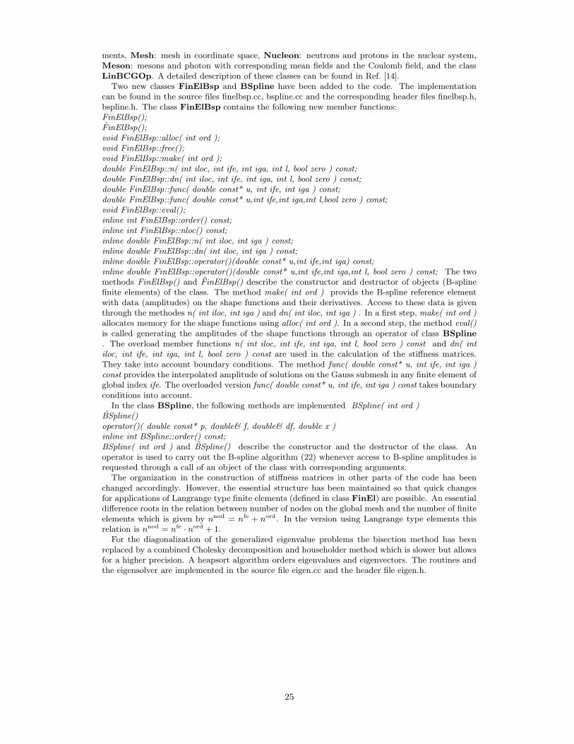
ments, Mesh: mesh in coordinate space, Nucleon: neutrons and protons in the nuclear system,Meson: mesons and photon with corresponding mean fields and the Coulomb field, and the classLinBCGOp. A detailed description of these classes can be found in Ref. [14].
Two new classes FinElBsp and BSpline have been added to the code. The implementationcan be found in the source files finelbsp.cc, bspline.cc and the corresponding header files finelbsp.h,bspline.h. The class FinElBsp contains the following new member functions:FinElBsp();FinElBsp();void FinElBsp::alloc( int ord );void FinElBsp::free();void FinElBsp::make( int ord );double FinElBsp::n( int iloc, int ife, int iga, int l, bool zero ) const;double FinElBsp::dn( int iloc, int ife, int iga, int l, bool zero ) const;double FinElBsp::func( double const* u, int ife, int iga ) const;double FinElBsp::func( double const* u,int ife,int iga,int l,bool zero ) const;void FinElBsp::eval();inline int FinElBsp::order() const;inline int FinElBsp::nloc() const;inline double FinElBsp::n( int iloc, int iga ) const;inline double FinElBsp::dn( int iloc, int iga ) const;inline double FinElBsp::operator()(double const* u,int ife,int iga) const;inline double FinElBsp::operator()(double const* u,int ife,int iga,int l, bool zero ) const; The twomethods FinElBsp() and FinElBsp() describe the constructor and destructor of objects (B-splinefinite elements) of the class. The method make( int ord ) provids the B-spline reference elementwith data (amplitudes) on the shape functions and their derivatives. Access to these data is giventhrough the methodes n( int iloc, int iga ) and dn( int iloc, int iga ) . In a first step, make( int ord )allocates memory for the shape functions using alloc( int ord ). In a second step, the method eval()is called generating the amplitudes of the shape functions through an operator of class BSpline
. The overload member functions n( int iloc, int ife, int iga, int l, bool zero ) const and dn( intiloc, int ife, int iga, int l, bool zero ) const are used in the calculation of the stiffness matrices.They take into account boundary conditions. The method func( double const* u, int ife, int iga )const provides the interpolated amplitude of solutions on the Gauss submesh in any finite element ofglobal index ife. The overloaded version func( double const* u, int ife, int iga ) const takes boundaryconditions into account.
In the class BSpline, the following methods are implemented BSpline( int ord )BSpline()operator()( double const* p, double& f, double& df, double x )inline int BSpline::order() const;BSpline( int ord ) and BSpline() describe the constructor and the destructor of the class. Anoperator is used to carry out the B-spline algorithm (22) whenever access to B-spline amplitudes isrequested through a call of an object of the class with corresponding arguments.
The organization in the construction of stiffness matrices in other parts of the code has beenchanged accordingly. However, the essential structure has been maintained so that quick changesfor applications of Langrange type finite elements (defined in class FinEl) are possible. An essentialdifference roots in the relation between number of nodes on the global mesh and the number of finiteelements which is given by nnod = nfe + nord. In the version using Langrange type elements thisrelation is nnod = nfe · nord + 1.
For the diagonalization of the generalized eigenvalue problems the bisection method has beenreplaced by a combined Cholesky decomposition and householder method which is slower but allowsfor a higher precision. A heapsort algorithm orders eigenvalues and eigenvectors. The routines andthe eigensolver are implemented in the source file eigen.cc and the header file eigen.h.
25
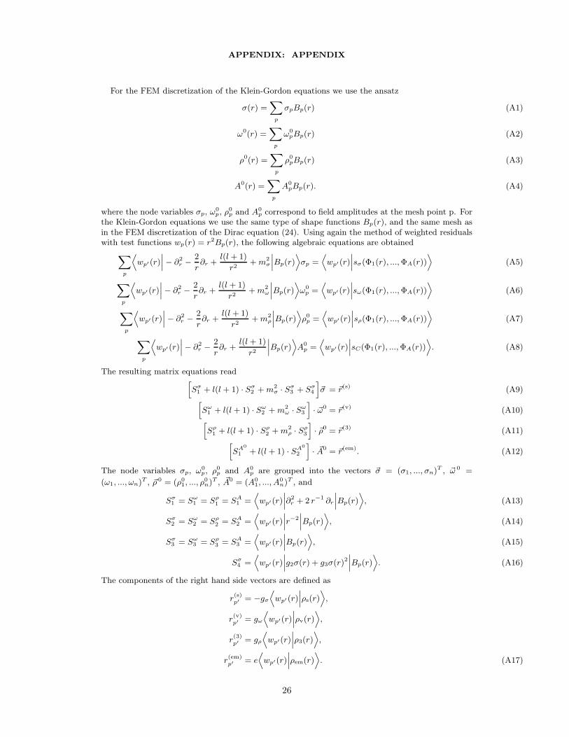
APPENDIX: APPENDIX
For the FEM discretization of the Klein-Gordon equations we use the ansatz
σ(r) =∑
p
σpBp(r) (A1)
ω0(r) =∑
p
ω0pBp(r) (A2)
ρ0(r) =∑
p
ρ0pBp(r) (A3)
A0(r) =∑
p
A0pBp(r). (A4)
where the node variables σp, ω0p, ρ
0p and A0
p correspond to field amplitudes at the mesh point p. Forthe Klein-Gordon equations we use the same type of shape functions Bp(r), and the same mesh asin the FEM discretization of the Dirac equation (24). Using again the method of weighted residualswith test functions wp(r) = r2Bp(r), the following algebraic equations are obtained
∑
p
⟨
wp′(r)
∣
∣
∣− ∂2
r −2
r∂r +
l(l + 1)
r2+m2
σ
∣
∣
∣Bp(r)
⟩
σp =⟨
wp′(r)
∣
∣
∣sσ(Φ1(r), ...,ΦA(r))
⟩
(A5)
∑
p
⟨
wp′(r)
∣
∣
∣− ∂2
r −2
r∂r +
l(l + 1)
r2+m2
ω
∣
∣
∣Bp(r)
⟩
ω0p =
⟨
wp′(r)
∣
∣
∣sω(Φ1(r), ...,ΦA(r))
⟩
(A6)
∑
p
⟨
wp′(r)∣
∣
∣− ∂2
r −2
r∂r +
l(l + 1)
r2+m2
ρ
∣
∣
∣Bp(r)
⟩
ρ0p =⟨
wp′(r)∣
∣
∣sρ(Φ1(r), ...,ΦA(r))
⟩
(A7)
∑
p
⟨
wp′(r)∣
∣
∣− ∂2
r −2
r∂r +
l(l + 1)
r2
∣
∣
∣Bp(r)
⟩
A0p =
⟨
wp′(r)∣
∣
∣sC(Φ1(r), ...,ΦA(r))
⟩
. (A8)
The resulting matrix equations read[
Sσ1 + l(l + 1) · Sσ
2 +m2σ · Sσ
3 + Sσ4
]
~σ = ~r(s) (A9)
[
Sω1 + l(l + 1) · Sω
2 +m2ω · Sω
3
]
· ~ω0 = ~r(v) (A10)
[
Sρ1 + l(l + 1) · Sρ
2 +m2ρ · S
ρ3
]
· ~ρ0 = ~r(3) (A11)
[
SA0
1 + l(l + 1) · SA0
2
]
· ~A0 = ~r(em). (A12)
The node variables σp, ω0p, ρ
0p and A0
p are grouped into the vectors ~σ = (σ1, ..., σn)T , ~ω 0 =
(ω1, ..., ωn)T , ~ρ 0 = (ρ01, ..., ρ
0n)
T , ~A0 = (A01, ..., A
0n)
T , and
Sσ1 = Sω
1 = Sρ1 = SA
1 =⟨
wp′(r)
∣
∣
∣∂2r + 2 r−1 ∂r
∣
∣
∣Bp(r)
⟩
, (A13)
Sσ2 = Sω
2 = Sρ2 = SA
2 =⟨
wp′(r)∣
∣
∣r−2∣
∣
∣Bp(r)
⟩
, (A14)
Sσ3 = Sω
3 = Sρ3 = SA
3 =⟨
wp′(r)∣
∣
∣Bp(r)
⟩
, (A15)
Sσ4 =
⟨
wp′(r)
∣
∣
∣g2σ(r) + g3σ(r)
2∣
∣
∣Bp(r)
⟩
. (A16)
The components of the right hand side vectors are defined as
r(s)
p′= −gσ
⟨
wp′(r)∣
∣
∣ρs(r)
⟩
,
r(v)
p′= gω
⟨
wp′(r)
∣
∣
∣ρv(r)
⟩
,
r(3)
p′ = gρ
⟨
wp′(r)
∣
∣
∣ρ3(r)
⟩
,
r(em)
p′= e⟨
wp′(r)∣
∣
∣ρem(r)
⟩
. (A17)
26

The nonlinear equation for the σ-field is solved in an iterative procedure. The nonlinear terms areincluded in the global stiffness matrix (see Sσ
4 in Eq. (A9)). In the iterative solution matrix elementsthat contain nonlinear terms are calculated using the field σ(r) obtained in the previous iterationstep.
APPENDIX: REFERENCES
[1] P.G. Reinhard; Rep. Prog. Phys. 52 (1989) 439.[2] P. Ring; Progr. Part. Nucl. Phys. 37 (1996) 193.[3] Y.K. Gambhir, P. Ring, and A. Thimet; Ann. Phys. (N.Y.) 511 (1990) 129.[4] G.Lalazissis, J. Konig and P. Ring; Phys. Rev. C 55 (1997) 1.[5] P.G. Reinhard, M.Rufa, J. Maruhn, W. Greiner and J. Friedrich; Z. Phys. A 323 (1986) 13.[6] D. Vautherin and D.M. Brink; Phys. Rev. C 5 (1972) 626.[7] J. Decharge and D. Gogny; Phys. Rev. C 21 (1980) 1568.[8] I. Tanihata et. al, Phys. Rev. Lett. 55 (1985) 2676.[9] W. Poschl, D. Vretenar, G.A. Lalazissis and P. Ring; Phys. Rev. Lett. 79 (1997) 3841.
[10] J. Dobaczewski, H. Flocard, and J. Treiner; Nucl. Phys. A422 (1984) 103-139.[11] K.T.R. Davies, H. Flocard, S. Krieger, M.S. Weiss; Nucl. Phys. A342 (1980) 111-123.[12] O.A. Marques; CERFACS Report TR/PA/95/31, Toulouse, France.[13] W. Poschl, D. Vretenar and P. Ring; Comput. Phys. Commun. 99 (1996) 128-148.[14] W. Poschl, D. Vretenar, A. Rummel and P. Ring; Comput. Phys. Commun. 101 (1997) 75-107.[15] W. Poschl, D. Vretenar and P. Ring; Comput. Phys. Commun. 103 (1997) 217-251.
27

0.0 0.1 0.2 0.3 0.4 0.5 0.6 0.7 0.8 0.9 1.0
-0.6
-0.4
-0.2
0.0
0.2
0.4
0.6
0.8
1.0
1.2
N
N
N
N
N1
2
3
4
5
(c)
Fig. 3 c

0.0 0.1 0.2 0.3 0.4 0.5 0.6 0.7 0.8 0.9 1.00.0
0.1
0.2
0.3
0.4
0.5
0.6
B
BB
B
B 1
2
3
4
5
(d)
Fig. 3 d
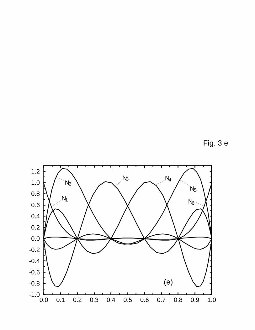
0.0 0.1 0.2 0.3 0.4 0.5 0.6 0.7 0.8 0.9 1.0-1.0
-0.8
-0.6
-0.4
-0.2
0.0
0.2
0.4
0.6
0.8
1.0
1.2
N
NN N
N
1
23 4
5
N6
(e)
Fig. 3 e

0.0 0.1 0.2 0.3 0.4 0.5 0.6 0.7 0.8 0.9 1.00.0
0.1
0.2
0.3
0.4
0.5
B
B B
B
B B
1
2
6
4 3
5
Fig. 3 f
(f)