)V( T )( H rr

The Finite Element Discrete Variable Method for theSolution of theTime Dependent Schroedinger Equation

B. I. Schneider

Physics Division National Science Foundation

CollaboratorsLee Collins and Suxing Hu

Theoretical DivisionLos Alamos National Laboratory

High Dimensional Quantum Dynamics: Challenges and Opportunities

University of LeidenSeptember 28-October 1, 2005

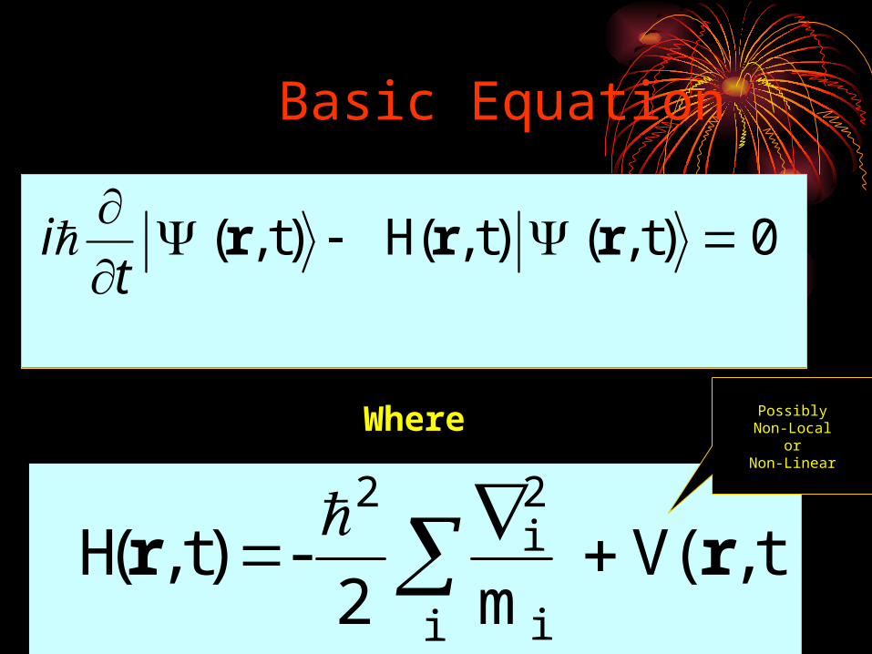
Basic Equation

t),V( m2

- )t,( Hi i

2i

2

rr

Where PossiblyNon-Local

orNon-Linear

0 )t,( )t,( H )t,(

rrrt

i

Objectives•Flexible Basis (grid) – capability to represent dynamics

on small and large scale

Good scaling properties – O(n)

Time propagation stable and unitary

”Transparent” parallelization

Matrix elements easily computed

Discretizations & Representations Grids are simple -

converge poorly

.quadratureby

done beonly can thesebasis expansionmany For

elements;matrix calculate toneeds One

)( C )(

ji

iii

H

rr

Can we avoid matrix element quadrature, maintain locality and keep global convergence ?

z)y,,x(

z)y,,x(

z)y,,x(

z)y,, x(

8/720 108/720- 1080/720 1960/720-

0 1/12- 16/12 30/12-

0 0 1 2-

* 1

z)y,,x(dx

d

ulasOrder Form-

7

5

3

es; DerivativSecond

)( )( )(

3i

2i

1i

i

2i2

2

i

h

ii r - rrr

Global or Spectral Basis Sets – exponential

convergence but can require complex matrix element evaluation

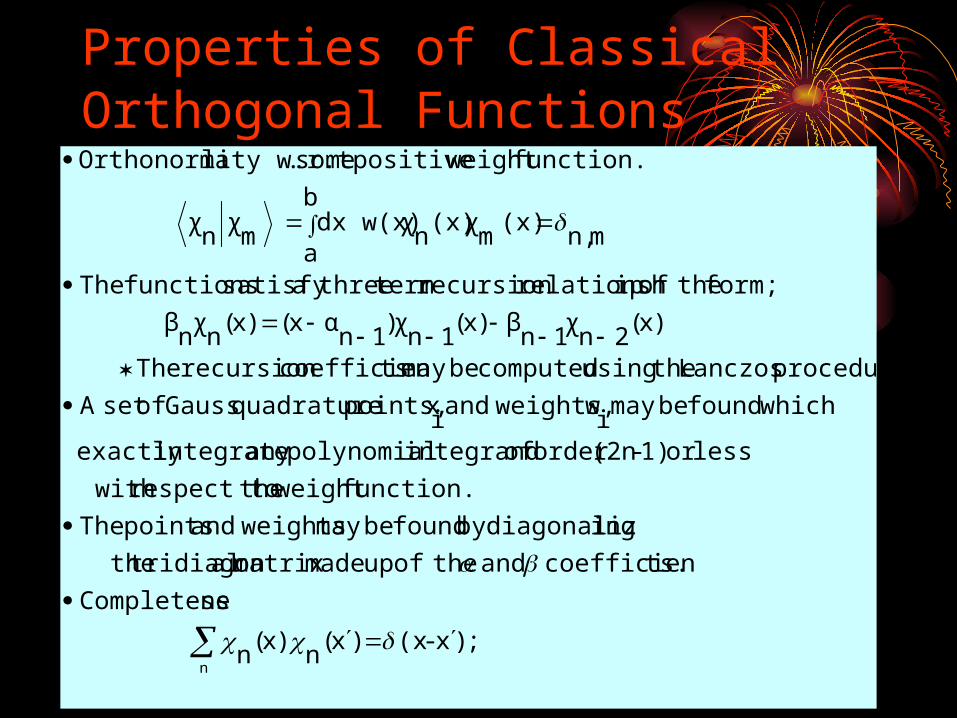
Properties of Classical Orthogonal Functions

; )x-(x )x(n

)x(n

ssCompletene

ts.coefficien and theof up madematrix al tridiagon the

ingdiagonalizby found bemay weightsand points The

function. weight therespect to with

lessor 1) -(2n order of integrand polynomialany integrateexactly

which found bemay i

w weights,and i

xpoints, quadrature Gauss ofset A

procedure Lanczos theusing computed bemay tscoefficienrecursion The

)x(2n

χ1n

β)x(1n

χ)1n

αx()x(n

χn

β

form; theof iprelationshrecursion term threeasatisfy functions The

mn, (x)

mχ (x)

nχ

b

adx w(x)

mχ

nχ

function. weight positive some .lity w.r.tOrthonorma

n

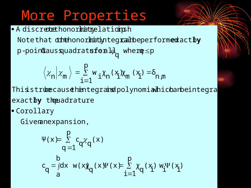
More Properties

p

1i)

i(x

i w)

i(x

qχ (x) (x)

qχ w(x)

b

adx

qc

(x)q

p

1qq

c Ψ(x)

expansion,an Given

Corollary

.quadrature by theexactly

integrated becan which polynomial a is integrand thebecause trueis This

mn,δ

p

1i )

i(x

m)χ

i(x

nχ

iw

mn

pq whereq

allfor squadrature Gausspoint -p

byexactly performed becan integrallity orthonorma that theNote

iprelationshlity orthonorma discreteA

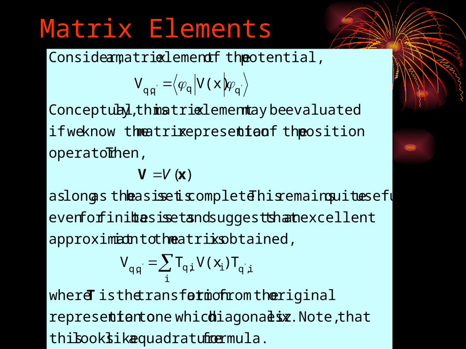
Matrix Elements

formula. quadraturea like looks this

thatNote, x. esdiagonaliz whichone totionrepresenta

original thefrom ation transform theis where

T )V(x T V

obtained, ismatrix the toionapproximat

excellent an that suggests and sets basis finitefor even

useful quite remains This complete. isset basis theas long as

)(

Then, operator.

position theof tionrepresentamatrix know the weif

evaluated bemay element matrix thisly,Conceptual

V(x)V

potential, theofelement matrix a Consider,

i,qii

iq,qq,

qqqq,

''

''

T

xV

V

Properties of Discrete Variable Representation

ion.approximatexcellent an be toappearsit practiceIn

true.is that thisassumed is its DVR, In the

mutiply)matrix andexpansion seriespower (Think

complete. is quadraturebasis/or theunless

)F(x F

toequal benot will thisgeneralIn

uF(x)u F

elementmatrix heConsider t

x uxu

and

w )(xu

hat,property t with the

)(x (x) w (x)u

functions, "coordinate" ofset new a Define

ji,iji,

jiji,

ji,iji

i

ji,ji

iqq

p

1qii

More Properties

points. quadrature Gauss theare i

xwhere

ij )j

x-i

x(

) j

x- x(

iW

1 (x)iu

tionrepresenta simpleA

i

ji

xx

u2dx

2d )x (iui w ju

2dx

2diu

:scoordinate Cartesian For .itsbut rule, quadrature

theusing evaluated bemay operators derivative theof elementsMatrix

trivial

Boundary Conditions, Singular Potentials and Lobatto Quadrature

Physical conditions require wavefuntion to behave regularlyFunction and/or derivative non-singular at

left and right boundaryBoundary conditions may be imposed using

constrained quadrature rules (Radau/Lobatto) – end points in quadrature rule

ConsequenceAll matrix elements, even for singular

potentials are well definedONE quadrature for all angular momentaNo transformations of Hamiltonian required

0

0.1

0.2

0.3

0.4

0.5

0.6

0.7

0.8

0.9

1

Fu

nct

ion

Val

ue

Coordinate

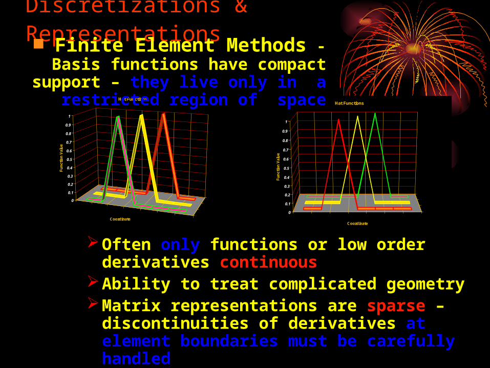
Hat Functions

Often only functions or low order derivatives continuous

Ability to treat complicated geometryMatrix representations are sparse –

discontinuities of derivatives at element boundaries must be carefully handled Matrix elements require quadrature

Discretizations & Representations

0

0.1

0.2

0.3

0.4

0.5

0.6

0.7

0.8

0.9

1

Fu

nct

ion

Val

ue

Coordinate

Hat Functions

Finite Element Methods - Basis functions have compact support – they live only in a restricted

region of space

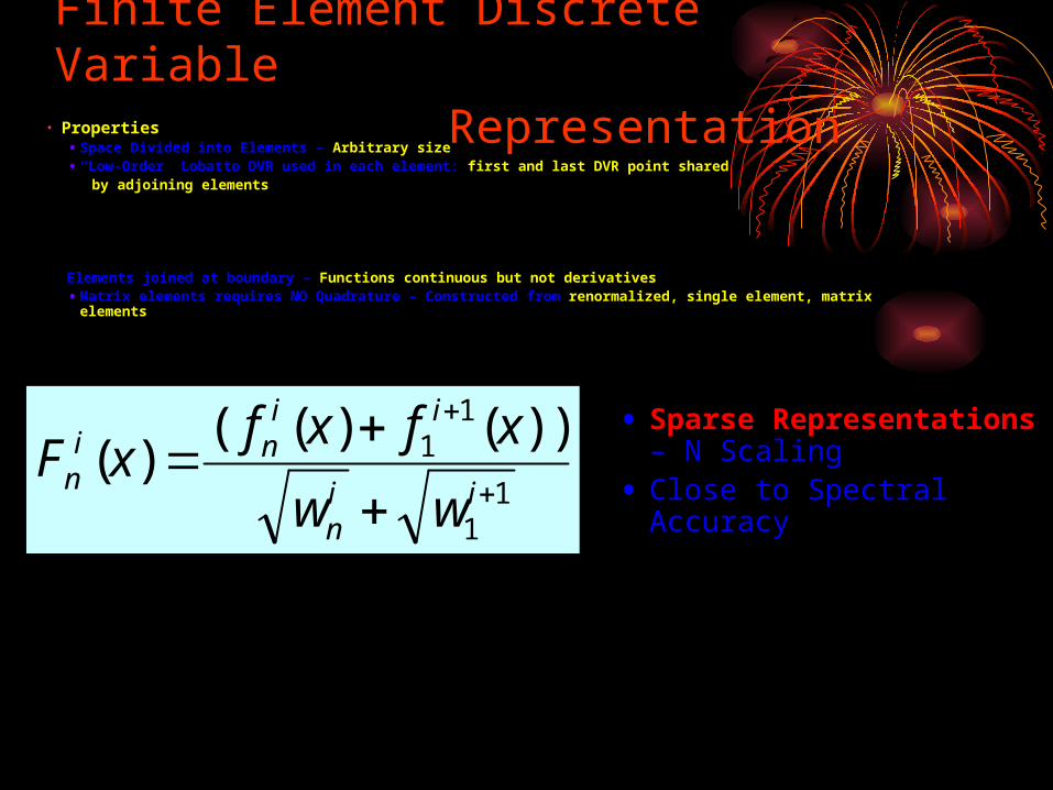
Finite Element Discrete Variable Representation

11

11 ) )()( (

)(

iin

iini

nww

xfxfxF

• Properties•Space Divided into Elements – Arbitrary size•“Low-Order” Lobatto DVR used in each element: first and last DVR point shared by adjoining elements

Elements joined at boundary – Functions continuous but not derivatives•Matrix elements requires NO Quadrature – Constructed from renormalized, single element, matrix

elements

• Sparse Representations – N Scaling

• Close to Spectral Accuracy

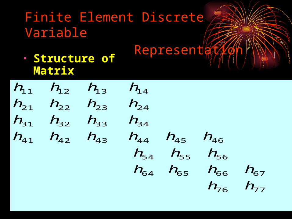
Finite Element Discrete Variable Representation • Structure of

Matrix

7776

676665

5655

64

54

464544434241

34333231

24232221

14131211

hh

hhh

hh

h

h

hhhhhh

hhhh

hhhh

hhhh

Time Propagation Methods• Lie-Trotter-Suzuki

1/3

22222

121

11

21

211

4-4

1p

)tr,( )(p)U(p U))4p-((1 U)(p)U(p U= )+tr,(

Phys.), Math. J. ki,order(Suzufourth To

ncalculatio hesimplify t enormouslycan choice judicious

abut arbitrary isn Hamiltonia theof breakup theNote

)tr,( )2

Ht )exp(-i

Ht exp(-i )

2

Ht exp(-i

)tr,( )2

()U2

( U= )+tr,(

accuracy,order second then to,H H H

)H exp(-i )H exp(-i )(U

Let

7776

676665

5655

64

54

464544434241

34333231

24232221

14131211

hh

hhh

hh

h

h

hhhhhh

hhhh

hhhh

hhhh

Time Propagation Methods

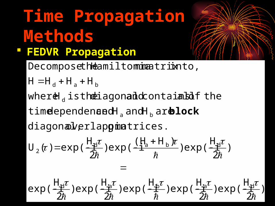
FEDVR Propagation

)2

Hexp(-i )

2

Hexp(-i )

Hexp(-i )

2

Hexp(-i )

2

Hexp(-i

)2

Hexp(-i )

)H (Hexp(-i )

2

Hexp(-i )(U

matrices. goverlappin diagonal,

are H and H and dependence time

theof all contains and diagonal theis H where

H H H H

into,matrix n Hamiltonia theDecompose

dabad

dbad2

ba

d

bad

block

t)ψ(r,2

t)ψ(r,t

i 22

m

Imaginary Time PropagationProblem Order

tMatrix Size Eigenvalue

Well 2 .005 20 5.2696

Well 4 .005 20 4.9377

Well 2 .001 20 4.9356

Well 4 .001 20 4.9348

Fourier 2 .003 80 49.9718

Fourier 4 .003 80 49.9687

Coulomb 2 .005 120 -.499998

Coulomb 4 .005 120 -.499999

Coulomb 4 .01 120 -.499997

Propagation of BEC on a 3D Lattice

Superscaling Observed: Due to Elongated Condensate

Propagation of BEC on a 3D Lattice

Almost linear speeding-up up to n=128 CPUs. It breaks down from n=128 to n=256 CPUs for this data set.

Ground State Energy of BEC in 3D Trap

Method No. Regions(X Basis)

Points Energy

RSP-FEDVR 20( x 3) (41)3 19.85562355

RSP-FEDVR 20 ( x 4) (61)3 19.84855573

RSP-FEDVR 20 ( x 6) (101)3 19.84925147

RSP-FEDVR 20 ( x 8) (141)3 19.84925687

3D Diagonalization 19.847

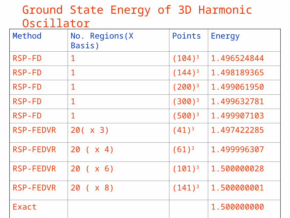
Ground State Energy of 3D Harmonic Oscillator

Method No. Regions(X Basis) Points Energy

RSP-FD 1 (104)3 1.496524844

RSP-FD 1 (144)3 1.498189365

RSP-FD 1 (200)3 1.499061950

RSP-FD 1 (300)3 1.499632781

RSP-FD 1 (500)3 1.499907103

RSP-FEDVR 20( x 3) (41)3 1.497422285

RSP-FEDVR 20 ( x 4) (61)3 1.499996307

RSP-FEDVR 20 ( x 6) (101)3 1.500000028

RSP-FEDVR 20 ( x 8) (141)3 1.500000001

Exact 1.500000000

Solution of TD Close Coupling Equations for He Ground State E=-2.903114138 (-2.903724377) 160 elements x 4 Basis

He Probability Distribution

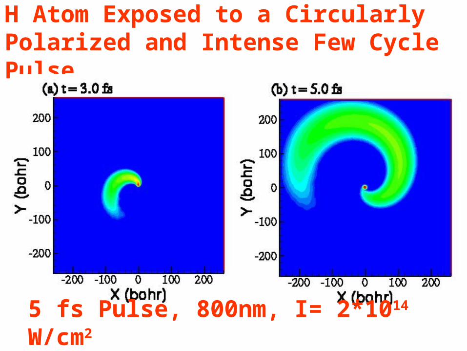
H Atom Exposed to a Circularly Polarized and Intense Few Cycle Pulse

5 fs Pulse, 800nm, I= 2*1014 W/cm2