axi-symmetric gravitational field part 2: … · %o.ff-am a4mm13~ m hm 3vui~ a i%piv inv mi...
TRANSCRIPT

-, UNLIMITED LTR 89022
C14
0 ROYAL AEROSPACE ESTABLISHMENT
Technical Report 89022
May 1989
QATI=I I IT1 MIATIftM IKI AKI%O.ff-am a4mm13~ m hm 3VUI~ a I%pIV INV MI
AXI-SYMMETRIC GRAVITATIONAL FIELDPART 2: PERTURBATIONS DUE TO
AN ARBITRARY J,?
by
D T IR. H. Gooding ELECTL
Procurement Executive, Ministry of Defence
Farnborough, Hamnpshire
fT1'wy 0 oP 0 UNLIMITED

CONOITIONS OF RELEASE0055705 BR-11 1982
*..... ...... U
COPYRIGHT(c)1988CONTROLLERHMSO LONDON
....... ........... y
Repors quoted ae not noftnooly available to members of tha public or to comerecialortgnlsatloe$
UNLIMITED
ROYAL AEROSPACE ESTABLISMENT
Technical Report 89022
Received for printing 5 May 1989
SATZLLITE MOTION IN AN AX-SYOZTRTC GRVTATIONAL FIELDPART 2: PERTURBATXONS DE TO AN ARBITRARy J
by
R. H. Gooding
SUMMARy
This Report Continues tht presentation of the untruncated orbital theorybegun in Technical Report 88063. The effects of the general Zonal harmonic,Jt , are now covered, the main x.sults being a trio of formulae for perturbationsin the spherical-polar coordinates introduced in the previous paper The formu-lae are only first-order in Jt , but, in conjunction with the second-orderresults for J2 published in Part 1, the complete et od formulae may be regar-ded as constituting a second-order theory, the Earth's J2 being ouch largerthan Jt for I > 2 .
The mean elements of the theory are defined in such a way that, for eachJt , the coordinate-perturbation formulae have their simplest possible form, withno occurrence of zero denominators. The general formulae are used in a rederlva-tion of the results for J3 , given in Part 1, and in a derivation of results forJ4 •
Numerical comparisons with reference orbits ate held over to a later report(Part 3).
Departmental Reference- Space 675
Copyright
Controller HM$O London1989
UNLIMITED

LIST OF CONTENTS
Page
1 INTRODUCTION 5
2 FUNCTIONS OF INCLINATION REQUIRED IN EXPANDING THE POTENTIAL 11
3 FUNCTIONS OF ECCENTRICITY USED IN THE SUBSEQUENT ANALYSIS 16
4 RATES OF CHANGE OF OSCULATING ELEMENTS 23
4.1 Semi-major axis 23
4.2 Eccentricity 25
4.3 Inclination 27
4.4 Right ascension of the node 27
4.5 Argument of perigee 28
4.6 Mean anomaly 29
5 SECULAR AND LONG-PERIOD ELEMENT RATES 31
6 PERTURBATIONS (SHORT-PERIOD0 IN COORDINATES - GENERAL CASE 34
6.1 The perturbation 6r 35
6.2 The perturbation 5b 39
6.3 The perturbation 6w 43
6.4 Universality of results (non-elliptic orbits) 47
7 THE SP' - 'ASES, AND INTEGRATION CONSTANTS 47
7.1 Mandatory constants for 6a 47
7.2 Constants for 6e and 6M 48
7.3 Constants for 6i and 6Q 50
7.4 Forced terms in 6w 53
7.5 Constants for Sa 57
8 RESULTS EXEMPLIFIED FOR Z FROM 0 THROUCH 4 60
8.1 The trivial (but exceptional) case t - 0 61
8.2 The t.livial case X - 1 66
TR 89022

3
Page
8.3 The case Z - 2 69
8.4 The case X - 3 71
8.5 The (new) case Z - 4 73
9 CONCLUSIONS 77
Appendix A Extension to the general gravitational fleld 80
Appendix 8 The quantities Bj,. and 80,1 in particular B6
Table 1 The functions AZ(i 8
Table 2 The constants a£k and a5t 89
Table 3 The functions B0(eY 90
Table 4 The quantities BZj 91
Table 5 The quantities Etk 92
Table 6 The number of terms in 6r , 6b and 6w 93
List of symbols 94
References 99
Report documentation page inside pack cover
Asoessieon re
NTIS SEMI
7T11 I NDTIC TAR 0
Justitleetlo
By -Distrbuitloa/
Availablity C~dsAvail andle,'
ist Special
TR 89022

5
1 INlTRODUCTION
This Report is the second of an intended trilogy devoted to satellite
motion about an axi-symmetric primxry, i.e. about a gravitating solid of
revolution. Thus it continues the exposition of Ref 1, which will henceforth be
referred to as 'Part 1'. Part 1 brought together the principles of an approach
to orbit modelling in which lengthy expressions for short-period perturbations in
the usual osculating elements are compressed into concise expressions for pert-
urbations in a particular set of spherical-polar coordinates; it then proceeded
into the presentation of a complete second-order theory for perturbations due to
the zonal harmonic J2 , and a complete first-order theory for J3 " When the
primary body is the Earth, J3 '(and every subsequent JZ ) is of order J2 ,, no
Part I may be regarded as dascribing (for J2 and J3 only( a compleie second-
order theory for Earth satellites, where 'first order' refers to effects of
relative magnitude io-3 . Though Part 1 has only recently been publishel, a
rbsuma2
of the theory had been given much earlier.
Two other papers are relevant to the maturation of the trilogy: a relent
one3 on mean elements (as used in Part 1), with particular reference to the
relation between mean semi-major axis and mean mean motion; and a much earlior
(and more important paper4, of slilar title to the trilogy's, that establisted
formulae for secular and long-period perturbations dae to the general JZ (so
general, in fact, that k could be negative, the formulae then being applicable'
to lunisolar perturbations). The present Report effectively combines the new
approach of Part I with the general principles and notation of Ref 4, the result
being a complete theory for the zonal harmonics; secular and long-period
perturbations are applied to mean orbital elements, and short-period
perturbations to coordinates.
Part 3 of tee trilogy will be largely devoted to the way in which the mean
elements evolve over periods of time longer than just a small number of orbital
revolutions. This topic, which was given limited attention in Part 1, is
entirel neglected in Part 2. It is intended that Part 3 will also give details
of the Fortran program(s) written to evaluate the accuracy of the overall
approach, using harmonies up to J4 • (The variations in the mean elements are
computed by a technique that involves a numerical component of an otherwise
analytical model, aspects of this technique were described in the paper5 that
originally outlined the author's philosophy of coupling a hybrid computational
procedure to the coordinate-perturbation approach.)
TR 89022
6
Other auttors have published first-order formulae for satellite
perturbations due to the geopotential; they usually address the subject more
generally than here, by covering the tesseral harmonics as well as the zonal
harmonics. The first entirely general results were derived by Groves6, in an
analysis of formidable complexity, whilst the classic eference is the text-book
of Kaula7. The very generality of the formulae a Refs 6 and 7 makes it
difficult to write down expressions for individual effects, however,, and it ia
not even easy to show that the two sets of formulae are formally equlvalent (the
full rirst-order expression for the perturbation in mean anomaly is omitted in
Ref 6, and the supplementary terms are only added as an afterthought in Ref 7).
Much of the difficulty in the general analysis arises from the need, when
covering the tesseral harmonics as well as the zonal harmonics, to allow for the
rotation of the primary. The uniformity of this rotation with time makes it
natural to work with M (mean anomaly), rather than v (true anomaly, as
integration variable,, but this inevitably leads to infinite summations. When the
analysis is restricted to the zonal harmonics, however, use of v (rather than M
leads to expressions that are free of infinite summation, and Zafiropoulos8 has
recently published untruncated formulae for the first-order perturbations in the
orbital elements due to the general Jt . The formulae of Ref 8 are much more
explicit than those in Refs 6 and 7, but this is unfortunately at the expense ,f
some very long expressions - it takes more than five pages to express the basic
formulae, aid even then the supplementary terms of the perturbation in M are
again absent. Now it will emerge from the present Report that the formulae of
Zafiropoulos can be expressed much more concisely. The real breakthrough comes,,
however,, when the short-period perturbations in elements are replaced by
perturbations ln coordinates. if it were not for the rotation of the primary,
this procedure could be immediately extended to the tesseral harmonics*; fc'r
orbits of sufficiently low eccentricity there is no difficulty, and very simple
general formulae were given in Refs 5 and 9, having originally been derived
during . stud;10
of Navstar/GPS.
AS w, -h Part 1,, a List of Symbols is appended to the Report; it is almost
entirely ciosistent with the List of Part 1, the few e.ception3 being noted. The
meaning of every new symbol is fully specified in the text, but only minimal
a Appendix A, which is in the nature of a posscript, outlines what is involvedin the extension for a non-rotating primary, and a separate paper is plannedfor later publication.
TR 89022

explanation is given for those carried over from Part 1. This in true, In
particular, for standard symbolism: thus we note, straight away, that the
orbital elements used are a, a, i, 0, w and M . an arbitrary one of which is
denoted (generically) by C ; also M - a + f e where f is s.iorthand for
fn dt , the integral being taken from epoch to current time. We continue to make
use of the quasi-elements V , p and L , realli only defined at the
differential level; thus, d(* dw c d (where c - cos 1 ),, dp - do + q dA
(where q2 . 1 - e
2 ) and dL- dM q d.
As explained in Part 1, each osculating element, , may be regarded as
the sum of a mean element, [ , and a short-period perturbation, 6 , so that
+ . (1)
A 'semi-mean' element, ,, is also needed (see section 3.2 of Part 1), but in
Part 2 we will usually ignore the distinction between Z and . The effect of
this neglect is that we do not distinguish between the quantities denoted by
6i , 6p; and SC in Part 1, normally using 6C here in the sense of SpC o:
Part 1; towards the end of the Report 'In deriving the perturbatione due to
J4 , in section 8.5), we remind the reader of the additional terms (split betdeen
4 and 6c , as explained in Part 1 that are needed to express 'first-order)
perturbations in full. Not even the distinction between osculating elements and
mean elements is of significance in evaluating the right-hand sides of equations
in general, since second-order perturbations are not taken into account in
Part 2, but the following important distinction (on left-hand sides) between
and t is worth noting: Lagrange's planetary equation for e constitutes the
starting point of analysis for the element 4 , whereas a formula for t is part
of the goal of that analysis.
The analysis is greatly facilitated by using, instead of w and u
(argument of latitude), the modified quantities w' and u' where
W' - W -+ and u' - u - 4. (2)
To avoid any confusion, it is remarked that the use of the accent (prime sign)
here has a connotation entirely different from that which distinguishes a
(osculating semi-major axis) from a' ; the lattr quantity is an absolute
constant of the motion '(under zonal harmonics only), whicn (as shown in Part 1)
TR 89022

constitutes the best choice for mean semi-major axis (9), to whatever order the
analysis is conducted. With u' now introduced, it is convenient to define herek hthe much-used quantities Ci and Sj ; thus*
Ck - cos Qv , ku, and sk - sin Qv ku'). 3)
When there is no ambiguity in regard to k , the superfix (but never the suffix
will often be omitted. (Warning: Cj and Si , as used in Part 1, identify with
c -2 and-_.2 here.)
As the primary is assumed axi-symmetric, we start from the potential
function a/r + I UZ , where the individual terms of the disturbing function are
given (in the usual notation by
uZ- - , (R/r)Z PZ(sin 0)
The value of i in the summation is norrally taken to run from 2 upwards, since
the cases i - 0 and Z - 1 are essentially trivial,, but the general formulae
to be developed cover the case i - I without difficulty; both 'tri ial' cases
are instructive and are interpreted in section 8, following Ref 4. if the
concept of an axi-symmetric primary is generalized to allow for mass outside the
orbital region, as well as inside,, then () can be extended to cover negative
, as in Ref 4; the only change needed in the expressirn for Ut i that Pt
is replaced by P-Z-I . Our overall requirement is to Integrate the planetary
equations for the general Ut , thereby obtaining the first-order contributions
to each 4 and 6 ,, and then to combine the ic (for the six elements) into
Sr, 6b and Sw ,, the corresoonding perturbations in the spherical-polar
coordinate system attacbed to the mean orbital plane; the latter is specified by
and I ,, and the transformation from the (r,b,w)-coordinate system to the
usual rectangular equatorial system is described in detail in Part 1.
In section 2 we decompose U, as
Ut U (5)
This notation leads to more concise expressions than if the trigonometricargument was jv + kw' , as was originally planned; the disadvantage is thatthe Kepler-conotant quantities are now C.k and .k , rather than CO and So .
TR 892

where 0 k 1 and U is only non-zero when k has the sane parity as
(or as -Z - 1,, in the extension to .< 0 . The decomposition arises as ,
in UZ ,, i effectively replaced by I , and this invo.ves the introduction of
certain '-.illes of inlilnation functions. The functions Ati I were originally
introduced in Ref 4 and are used again,, but quantities Atk , proportional to the
Ak(i values, are actually more convenient. Related functions, and assoaiated
quantities, are also introduced, and recurrence relations are given. These
relations (and corresponding relations for the eccentricity functions, referred
to in the next paragraph) are required here in the development of the theory, but
they are also important as computational aids in the Implementatio f the
theory. The U can be treated separately in all the analysis up to the
derivation of the 6r and the 6w ,, but there is a complication in the
derivation of 6b ; this will be handled by the introduction of another index,
K , which is always of the opposite parity to Z (and hence k0.
* Following the elimination of 6 , we must also eliminate r , using the
basic formula of the ellipse
S + 0 0cosv, (6)r
before the planetary equations can be integrated. This involves families of
eccentricity functions, which are introduced in section 3. The functions BI(e)
were originally introduced in Ref 4, but the quantities BRj ,, proportional to
them, are actually more useful. Recurrence relations are given, and these are
even more important then the ,elationu for the inclination functions. !t is
implicit in the use of the Btj that every Uk could be further decomposed,
into Uki say, but we prefer not to do this, postponing the introduction of
the Rj until Ut , in each planetary equation, has been eliminated in favour
of an explicit expression. thus the notation Uk is not
The development of each planetary equation, via first the Atk and then
the Bj , is the topic of section 4. As already rmarked, we avoid infinite
summations by retaining v as an argument of the equation (as opposed to
eliminaLing it in favour f M ), and indeed we make it the integration variable
by applying the relation
d- n q-3 (p/r)
2 (7)
rR 89022

Each equation now expresses d /dv rather than , as a (finite) sum of terms
In v . Each such term is just a multiple of 9 , or S, as it turns out, so
the integration of the equation is immediate. Terms with k + j 0 lead to the
6C by definition. Terms with k + J - 0 , on tle other hand, are effectively
constant over the short term, and contribute directly to ' ; when k - 0 (and
so also j - 0 ), the integrated contribution is a secular perturbation, whilst
the terms with k 0 0 contribute to the long-period perturbation. The
dintinction is important for Earth satellites, because the secular variation of
w (due to J2 ) must be allowed for In integrating the perturbation, but the
subject was dealt with in Part I and will be picked up again in Part 3; there
will be no further reference in Part 2 to this coupling between J2 and the
other J.
Formulae for the lk (C due to Uk ) are collected in section 5, whilst
the reduction of the appropriate 6 to formulae for 6r , 5b and 6w is the
subject of the next two (and much longer sections. As described in previoun
paern there is an important distinction between the integrations required for
the t4, types of term: for the k . the process leads to definite integrals
(see Parta 1 and 3). necessarily zero if taken over zero time from epoch; in
Zk-components of the 6C , on the other hand, the process leads to epoch-
independent indefinite integrals that (apart from the complication of nemi-mean
elements) satisfy '(1). aut indefinite integrals contain arbitrary constants,,
where a 'constant' in the present context is any quantity that is independent of
the fast-varying v , i.e. would be a true constant for motion in a fixed
ellipse. It is only when theme constants are all assigned that (at the first-
order level) the mean elements, , , are fully defined.
It ham been noted that enormous advantage accrues from taking ' to be the
exact quantity a' (defined by the energy Integral, as explained in Part 1), but
there are no immediately compelling reasons for associating particular constants
with any of the other five elements. We therefore base our choice on the
philosophy of making the expressions for 6r ,, 6b and 6w as simple as
possible. These expressions, which constitute the most important results of the
Report,, are presented in their general form in section 6; each of the three
expressions involves a summation over the index J, with the integration constants
for tae elements (other than a ) not yet taken into account.
TR 892

In the general formulae just referred to, certain values of j in the
summations would involve terms of zero denominator, and it is by the eliminatior
of all these terms that the integration constants (other than for a I are
chosen. This is the subject matter for seotion 7, which completes the entire
analysis. An outline of the material in this section is as follows. First,,
the formula for the mandatory constant in 6a (for each Uk ) is reoorded,essentially as a matter of completeness. Second, the constants are derived for
6e and 6M that validate the omission of the terms with particular j that
would otherwise arise in 6r . Third, the constants are derived for 61 and 6Q
that do the same thing for 6b . Fourth, special terms (with particular j )
in Sw , that could not be included in section 6 because t.y are induced by the
constants in 6e and 6M , are obtained. Finally, the constant in 6W (for
earh Uk ) is derived.
Examples of the general formulae of section 6, together with the special
terms in kw derived in secticon 7, are given in section 8: first,, for the
trivial oses t - 0 and t - 1 , the interest in which 'as been remarked; then
for Z - 2 and Z - 3 , leading (as a useful overall checex to results already
known from Part 1; finally, fo" Z - A , leading to formulae not hitherto
published.
2 FUNCTIONS OF INCLINATION REQUIRED IN EXPANDING THE POTENTIAL
Following Ref A, we expand PZ(sin 6) , required in '(), via the additiontheorem for zonal harmonics (or Legendre polynomials); thus
Ft(sin B) 11 U kt T-7T a)' % u 8k-O
Here u0 1 ,u k -2 if k > 0 ,and the Legendre function Pk is defined by
Pk(c)
• ds p(c)Z1 c dck
TR 89022

f
12 The second factor (the k'th derivative in (9 is a polynomial in c fwhich '(with k I t) does not vanish when c - 1 , its value then being
(t - k)/({2k k1 (t - k)1) . Hence this factor may be normalized", in a certain
useful sense, and we write
dkPj(c) ( - k)l A(i), (10)
dek
2k kl (i -k)l Z
where Ak(ij is a pure polynomial n s C- sin i if k has the same parity as
Z but has an adlitional factor a if k and t are of opposite parity; in
each case the constant term in the polynomial is unity,, by the normalization.
Explicit expressions for the A(i) are given in Table 1, for values of Z and
k up to 6.
We can now rewrite (8) as
PL(3in )" alk sk A(ij Au' , (11)
k-O
where the constant, alk , is given by
tik - uk P(0) /(2k k1 .'(12)
A different constant,, Ck , was used in Ref 4, incorporating a factor associated
with the eccentricity functions of section 3; it is given by -2-k (i 1 ) t, ,
where (m) is the usual binomial coefficient, m here (and throughout the paper)
being used to denote a general integer, with negative values allowed; when
0 , in (12) must be replaced by P.tj ,, so that ak - , but the
relation of s£a to the of Ref A is unchanged. It is clear, from the lastpr t () or Pk .(O)) vanishes when k and i (or -Z - I ) areparagraph,+ that P()(rp
of opposite parity,, and it tay be shown thet when the parity is the same,
This 'normalization, which nas nothing to do with th- standard normalization of
the spherical harmonics and their J-coefficients, leads directly to AC(i) - 1
one of thy pair of starting values for the recurrence relation (21). .or some
purposes a different normalization is preferable such that A(i) is defined
for all i 0 . and A6(i) - I ; the family of normalized functions can thenbe extended in a unified manner when the orbital theo-y is to cover the
tesseral harmonics (Appendi A). 8
TR 09022

! 13
(-) 21 (j+9Z W )! (+(T.- k.))' (3
In substituting (110 into (0i it is of great benefit to introduce a new quantity,
AU 1, defined by
A9.9 - J, (R/P). atk a
9 Ak(i)' 14l9)
where p C - a(1 - e2)) Is the semi-latus rectum (or parameters of the orbit;
the equation applies when I < 0 , so long as the suffix of A is replaced by
-t - I . The use of Ak permits us to write the general term of (5(. using
also the notation of (3), as
U - - ( p/r)t.
Aik c . (150
It will be noted that, whereas Ak(i is defined and useful regardless
of parity, A (and hence Uk ) is only non-zero when k and 9 are of the
same parity. The zeroes come from a1 k 9 for which the non-zero values, up to
k - t - 6 . are given by the like-parity entries of Table 2. (The Table has been
extended back to Z - -7 , to illustrate the identity of atk with a-X-lk when
t < 0 .Y However, a use will be found for quantities that behave in the opposite
way from atk and Aik , anticipating which we define (with bold letters to make
the distinction)
t - u. ( -t 1 1) P:, ( 0 ) /( 2 K c 9) (16)
and
a dA t e , J 9 . ( A / p ) .
a t ,e S K A f i ) ( 1 7 )
where k has been replaced by K to signify tnat we now have quantities that
are non-zero only when K and Z are of opposite parity. alf of Table 2
(for all Z ) is devoted to au. , since these quantities can be included with
atk on a chequer-board basis.
TR a9e22

I!14-
We will require derivatives of the inclination functions. It is evident
from (10) that
dA - t( k 1) s<di1 * 1) A1 Z i (18)
from this and (10, it follows that the (partiall derivative of Alk with respect
to I is given by
At'k - JZ (R/p)t 'tk sk" 1 A - (i- k)(9. k Tk-A-i-- 1 f , (19)
where f - s. , The quantity in '(Curly) brackets is the D (ij of Ref 4. We
will also require, finally, the particular combinations of A1 k and A&
denoted by Alk and Ak , and given by
Lk - ks"1 Aik 1 0
-1 A&k 1 (20)
the 3-1 and C-1 factors do not imply singularities, as they must always
cancel via k Atk ann Alk respectively.The A (i) and tA (and hence the At 1 may be computed with the aid of
recurrence relations. A fixed k was stipulated in Ref 4 for the formula
(I k* Ak A(i( - (2j - 1) c Ak_ '(i) - ',(t - k - 1) Ak.2 i , (1
valid for t. k + 2 with the starting values Ak(ij . 1 and Ak,1(i) -
(211 is even valid for A - k + I , if an a-bitrary (but finite) Ak_1(0 is
assumed. However, it is usually more useful to stipulate a fixed A the
required formula wan giver by Merson11, being
Ak(i) - c AkIli) _ ( - 1)( + k 2) Ak*
2(i) '(22)
valid for X - 2 1 k a 0 with the starters At(i) - I and At-1(i) - c
(22) is also valid for k - t - I , with an arbitrary (finite) At*'(i) . Either
of the two preceding 'pure' three-term recurrence relations, (2) or (22), can be
used with JLst one 'mixed' such 'elation to generate all the relations connecting
the Ak(i) ; perhaps the simplest mixed relation (with neitner Z nor < fixed)
in
TR 29022

hI
15
'(Z )a. ki4 ) A1
Ci 2k Ak_1(lj .23)
For the 04k we have the relation, for proceeding along a 'fixed diagonal'
of Table 2 (with Z > 0 and a constant value of t -k ),
4+k-1a4 k Uk. k a.-1,-1' (24)
whilst to proceed to a lower diagonal we have
u k (k+Iak - -_____k_'(25)
These relations suffice to generate all the atk from 0,0 Similar
reuatlons permit the generation of all the a1k from I,0 -1 , they can be
dispensed with, howew', since it follows from (12), 13) and (160 that
au K a ' z (26)-£ £1, - - £1,
Though it is the Ak '(and At, ) that we actually require to carry through
the paper, recurrence relations are not offered for these. To preserve parity if
one suffix is fixed, it would be necessary to use alternate values of the other;
there seems little point in doing this, though a valid relation could easily be
obtained, for example by applying (21' three times. There are simple relations
between the Alk and AU , however. We will need two of these in section 7.3,
namely,
z - .&L1J 2kcs1 A
(27)[Uk I Uk I Uk
and
1,1.1-- - A 1- 1 - 2 , (20)k+W - u4
Postscript. in regard to equations (27) - (31), it should have been noted thatA4k/Uk and A1k/uk actually reduce to -Zo
-o A 4.1/Uk1. and Zc
-1I A, k uk.1
respectively, results that are implicit in the a'nalyss of section 6., the u,factors could be avoided by allowing negative k and * (see the footnote ofpage 40).
1R 890Z2

!1i
16
these being true for 1 j k I X (with I and k of the same parity. For
F k - 0 we only have one relation, given by direct addition of (27Y and (28) (and
really only one, involving direct subtraction, when k - Z ); thus,
tkA,1 - - 2AZo . (29)
We could use (27) and (28) to obtain expressions for A±k I defined by
(20),, but instead derive them directly. On substituting for Ark from (14) and
for Atk from (19, then in forming Aik we find that the term in AZ(i
cancels out and we get (for 0 g k ., and Z and k of like parity)
p) - k)(i - k 1) C-1 Sk.l A 1(i) . (30)Atk . J, (R/P)Z atk 2(k + 1) Z
For AaV , on the other hand, the combination of Ak(i) and Ak (iy is such
that ,(22), with k replaced by k - l, is immediately applicable, leading to
(but only for 1 k I z now
A k . 2k J4(R/p)t
a1k o-1 3k-1 A1i(i) 31)
for k - 0 , tis would give a false value of zero, the correct result being the
same as is given by 30, since A+,0 - -A-, . The formulae (30 and (31) are
used in the analysis of 6b in section 6.2. (See also the footnote to page 15.
3 FUNCTIONS OF ECCENTRICITY USED IN THE SUBSEQUENT ANALYSIS
The term Uj of the potential, specified by C4), has now been decomposedinto the Uk defined by (15), the latitude (0, having been eliminated. The
longitude was absent from U, from the beginning, because of axial symmetry,, zo
it rea.na to eliminate the radius vector (r) . This can be done by appeal to
(6), but (as noted in section 1) we will in practice postpone the use of (6)
until the setting up of each planetary equation, so the present section is
preparatorj in nature. Further, it is not (p/r)IC1
, in (15), that must be
eliminated, but (p/r)1-1
, an a factor (p/r)2
is retaned to effect the change
of integration variaole defined by (71.
It is evident from (6) that an expansion of the form
(p/r)I1
-1 uj 3xj cos jv '(32)
J.o
TR89022

F ........ I -
is possible, for Z Z , and we regard B j n defined by this expansion;
arly, Btj I a polynomial in e . We shall find it useful, and entirely
natual, to extend the definition of Btj to negative j , by defining
SEJ -BtljI , and to take Bij - 0 when IJI Z I . On this basis, and using the
notation of (3), we can replace 32) by
-P/r)I'1
B tj CO , (33)
where the summation effectively runs from j - -- to J- s- o that there is
no need for explicit smation limits.
To make use of soe results fron Ref 4, we first demonstrate that the Bzj
are directly related to the Hansen X functions of classical celestial
mechani s12 ,
such that
Btj - &- X0 -ij %34)
Hansen's functions '(of eccentricity are defined (uniquely) by the existence of
the expansion,, for all integral Z and j ,, regardless of sign,
(r/a)l exp(Jv), - X exp(%Mm) (35)
where 12
-1 and the smatton runs from -- to +- Only when m - 0
which is the case with which we are concerned, is X J
a simple (finitely
expressible in eleventary functions) function of e (and it is precisely becausf
of this that we change the variable from t to v in the planetary equations,
thus avoiding infinite expansions in M ).
To demonstrate ,(30, we first replace the index I by -(9 + 1) in '(35),
and then integrate over a revolution of M . We get (from the real part of the
result
c (P/r) os jv dH - 21 q2(t+Q x6z-t,J (36)
0
Tv 89022

But from (33),!S~'(l).+l cos iV dM f B ~, (p/r)
2 c0s my cosn jv dM (37Y '
2I 2m
0 0
We apply (7) to change the integration variable to v on the right-hand side of
(37); only if m - ij do we retain a non-zero term, and in fact
2%
f cos jv dM - 2w q3 B tj , (38)
0
Then (34) is immediate from (36) and (38).
Some comments related to the notation are worth makJ .& before we proceed
further. In principle we are reserving the suffix k for the A functions and
J for the B functions, but ii section 5, where only the value -k arises for
J , we will naturally encounter Bk . We would also rather naturally change the
notation from j to k in (35) if we w~re following the traditional path7 in
which the integration variable is M and the expansion of (15 is by 35Y
directly. After replacement of 9 by -(t 1); ,, the Hansen function would then
appear as X;Z-l<k
, which is nowadays (following Kaula7) usually expressed (when
Z 1 0 as Gtpq(e) ; here p - f( - k ,: wbich must be integral (assuming t
and k to be of the same parity), and q - m - k . Introducing also the
notation Gtq , which the present author9 has recommended as preferable to
Otp1 , we may extend (34) by writing
q- 2M-I) Bij - X6£'-"
J * Gi,i(t..j ,.j(e) - Gj,_ (e) . 0 9)
Gooding and King-Hele13
nave recently reported o" the G functions that are
relevant to resonant satellite orbits, Ref 13 includes the listing of a Fortran
program (by Alfred Odell) that computes the functions for arbitrary values of
Z., k and Kaula's q , by quadrature.
We can now use the identity (34) to tie into the inal~sis of Ref 4. Thus,
we may express the e-polynomial Btj , when Z Z I and 0 j < Z , in terms of
a normalired such polynomial, the connecting relation being
hj - (t ] 1) (e/2)J B(e) (40)
TR 89022

A4(e) in (40) is a polynomial in .2 with constant term unity by the
normalization. Explicit expressions for the BI(e) are given in Table 3, for
values of Z and j up to 7 and 6 respectively. There is an evident
resemblance between the B0(e) and the Ak(i) , a significant difference being
that the new functions run from Z - 1 and not t - 0 ; the resemblance is not
fortuitous,, since it can be shown that4
oj(e)- a4! rL&.j. "1 +134,2
(se/2,-' q'-' PI.l(q-1 , (h
from which it follows that
eW - qZ-J-1 Aj.l(tan-lte . '(42)
In contradistinction with the Atk , however, it is usually much better to
work with the Btj directly (in recurrence relations, for example),, rather than
through Bi(e and (40. One reason for this is that only alternate values of
the A9 k are non-zero, whereas (for Ii < Z and e O all the B0j are non-
zero. Further, no difficulty arises with the gtj when j < 0 (as already
nored, and see also Appendit B), whereas B4(e would then be infinite (If
[li < V.) We can even allow Z to be negative (or zero, as well as j . The
validity of this follows from the universality of 34) - the universality is
brought out by Table 4, which lists B£ for x running from -3 to v4 and J
from -1 to -3.
The entries in Table 4 form triangular blocks of four types. First, for
> 0 and iJi < t , we have the quantities that can be expressed by (40) rhen
J 2 0 . Secondly, for Z > 0 and JI ? Z9 , we have (two blocks of) zeroes.
Thirdly, for Z S 0 and lJI S -Z , we have quantities that, when j Z 0 , can be
expressed by a formula complementary to (40), viz
B " (9.31) (e/2)J q21-
1 Bjt 1(e)
(93)
a formula equivalent to this was given in Ref 4, the aprlication being '(as noted
in section 1) to secular aid long-period perturbations associated with exterior
(rather than interior) mass. Finally, for 9 5 0 and 1JI > 9 , we have (two
blocks of, quantities that are most conveniently expressed in terms of 8 (not
now denoting latitude, as previously) and q , rather than e and q , where
TR 89022

1 q (4Y
no attention w-is paid to these quantities (or their equivalents), in Ref 4, there
being no appl~cation for them, but the formula for Boj is der/ed here, for
completeness, in Appendix B. (Other entries in this last pair of blocks are then
derivable frm recurrence relations. Before leaving Table 4, we note that the
formula for the X or G function corresponding to Btj Is immediate from the
Table, in /iew of ,34); tnus it is only necessary to apply the factor q-21
which introduces a negative power of , when there is not one already present
and cancELs it out when there isl
In regard to derivatives of the eccentricity functions, it can be shown (by
working from (41)), and easily verified from Table 3 that, for I S j < z
de[4Bi(e)l - 2ie-1 (Bi-le)' - Bi() '(45)
The universal formula for the derivative of B11 is
Bj- (1 - ) Bt.1 ,j_1 - J e1 B1j '(46)
For I S j < t , this follows from (45); for general entries in Table 3, it can
be verified with the aid of q' and a' , which may be expresied as -e/q and
B/eq respectively. However, because we only !ntroduce the Btj after each
planetary equation has been set up, we effectively only use (46) in expressing
the rates of change of tne mean elements. Since this involves
ae(q AUA BO - q-1
Zk {q2 8ik + (21 - 1) e Btk, (7
we defln
Etk q2 B - (21 - 1) e Bk (48)
then (46), re-expreased via the :ecurrence relation (56), leads to
Ekk e -1 (
1e2 - k) B41k (t - k) Btk-I . (49)
TR a9022

141 21(By symmetry, there is a parallel expreanion-o Eo M that involvesn t and
.1k- ) Table 5 given explicit expreasions for the BE , with 9X running
troa,z'3 to +'4 as in Table 4i; only the entries in which k haa the name parity
an 9. (or -V.- 1 It I9< 0 ) are useful in practice, and entriea for k. .9. (or
* -9. + I It 9Z S 0 ) are omitted entirely (for k. k 9. > 0 they would all be zero).
The Ekk9 are related to the E (e), of Ref '4 by
El e-1 (e12)
9. (9. - 1) Ek(e) (50),
when Z> 0 ;tor Z9. 0 ,the extra tector q24+1 in required (of (443), where
the additional factor, In relation to ('40), ia q2Z.1
i
The B~ nay be computed tree recurrence relationa for the 81(e) , which
will now be given, but in developing the theory It in more useful to have such
relations for the B9.3 themnelves, no thene will alsc be given. For fixed
90), the recurrence tormula (trom Ret 14) in
(9. + 1 0 BI~ (e, - (2t. - 3) Bi-, - (Z. - 3 - 2) q2
BJ_2(e) (1
valid tor Z. Z. J 3 with the ntarterns~1'e and BJ,2(e) both unity. For
tixed t. C Z 3), on the other hand, the tormula is"
81(e) - B41
(e) 'a (9 7 1- 2(). 1) el B4 2(e. (52),
valid fcr .-39 3 9. Z0 with the ntartern B'_'(0 end BI-2(e) again both
unity. The resemblance ot (51) and (52) to (21) end (22) respectively tollows
trom the remark leading up to ('42).
The recurrence relations for' the B9.3 , that correnpond to (51 ( and (52),rea pectively, and are valid for all Z. and , are (when symmetrically
expreased)
9.(9 - 1) q2 B L- 1,'j - t(2. - 0) B9.3 + '(t.2 - 32) B9.,1, ' 0 '(53)
and
Q aBtj- +2jBj Q+ ) B~ l- 0; (54)
Tn e902z

22 Jthe mandatory symmetry in (54), to satisfy the unchanging value of Btj under (1
the operation J - -j , is evident.
As remarked for the Inclination functions, either of the 'pure' relations,
(53) and (54), can be used with a 'mixed' relation* to generate all tte
recurrence relations connecting the B Here the mixed relations are, in
particular, those that connect three out of four of the B zj lying 'around a
square' of index duplets; if the square consists of the duplets (t, J),
(t - 1, J), (Z, j - 1) and (t + 1, j - 1), then the four mixed relations
connecting them '(all of which we shall require in the sequel) are
t B - (z, - J) S+, * le B,j+l - 0 , (55)
iq2 B8j - a J), B+I j + (i + J + 1 Y e Bt,+1,j+ - 0 (56)
te Bj + z Bj- 1 - ,(z + J + 8 ) BL I J+ I - 0 ,(57)
and
(Z - j) e B i,j + Zq2
8 -,j+l - (I + j + 1) Bi+l,j+ I 0 (58)
If we re-order the terms in the last two relations and replace J by J - I , we
get relations which are symmetric pairings of (55) and (56)', viz
z Bj - (a J) Bl.i,j + I e Bj_ - 0 (59)
and
tq2 B j - (t + j) B1+1 j + (8 - 1), e BZ.l,j- 1 - 0 . '(60)
Of this set of relations, (55) and (59), can be obtained at once from (54) and the
relation equivalent to one give% ',(for the Hansen functions)' by Zafiropoulos8, viz
ie '(Bt,1. - Bt,j+i) - 2J 88,I.J (61)
this is of a different 'shape' from our triangles-around-the-square relations,
but is perhaps the simplest recurrence relation of all.
Note added in proof: Ref 19 indicates that, for inclination functions, purerelations are computationally prefer-.ble to mixed relations (see also Ref 20).
TR 89022
'~1 234 IATES OF CIANGE OF OSCULATING ELEMENTS
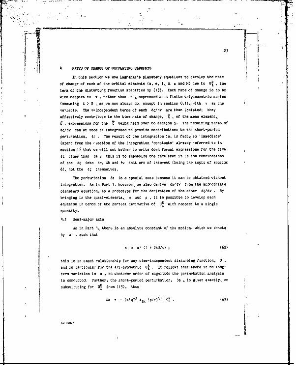
In tnis section we use Lagrange's planetary equations to develop the rate
of change of each of the orbital elements (a, e, i 0, w and M) due to Uk , the
term of the disturbing function specified by (15). Each rate of change is to be
with respect to v , rather than t , expressed as a finite trigonometric series
(assuming Z > 0 , as we now always do, except in section 8.1), with v as the
va-iable. The v-independent terms of each d /dv are then isolated; they
effectively contribute to the time rate of change, ' , of the mean element,
Z expressions for the t being held over to section 5. The remaining terms of
dC/dv can at once be integrated to provide contributions to the short-period
perturbation, Sr . The result of the integration is, in fact, so 'immediate'
(apart from the 'uestion of the integration 'constants' already referred to in
section 11 that we will not bother to write down formal expressions for the five
it other than 6a ; this is to emphasize the fact that it is the combinations
of the 6 into 6r, 6b and iw that are of interest (being the topic of section
6) , not the 6 themselves.
The perturbation 6a is a special case because it can be obtained without
integration. As in Part 1, however, we also derive da/dv from the appropriate
planetary equation, as a prototype for the derivation of the other d;/dv . By
bringing in the quasi-elements, ) and p , it is possible to develop each
equation in terms of the partial derivative of Uk with respect to a singla
quantity.
4.1 Semi-major axis
As in Part I, there is an absolute constant of the motion, which we denote
by a' , such that
a - a' ( * 2aU/) (62)
this is an exact relationship for any time-independent disturbing function, U
and in particular for the axi-symnetric Uk . It follows that there is no long-
term variation in a , to whatever order of magnitude the perturbation analysis
is conducted. Further, the short-period perturbation, ia is given exactly, on
substituting for Uk from (15), thus
6a - 2a'q-2
Ak (p0r)t C . (63)
TR 89022

%i
This does not mean that an exact perturbation can be written down for semi-major
axis, however, as the right-hand side of (63) is expressed in terms of osculating
elementr- as soon as mean elements are introduced, the result is no more than a
first-order perturbation expression, as with any other ; .
C, To present 6a in the form appropriate ior use in section 6.1, we combine
Swith one of the factors p/r Thus,
6a . -aq-2 Ak (p/r)t (eC~k 2C eCl) .k) (6
We retain another p/r factor explicitly, and expand the remaining (p/r)t 1
by
(33). By this means the term 2C0
, for example, in (64) is effectively
transformed, f'or each J ,into * C_ . But each pair of terms '(such as
this) for positive J , in the infinite summation of (33), is matched by the same
pair (in reverse order) for negative j , so we can express the result of the
6a - - aq"2
Atk (p/r), B B1j (eCj.I + 2Cj + eCj+I ) . (65Y
We now develop an exprcision for da/dv ab initio, using the general
procedure that involves the planotary equation for & . This equation is
da 2 3Udt mra T (66)
and on substituting for Uk
we get
da -2naq.2 Au M(p/r)t* CO) 6-t
The M-differentiation is immediate, since p/r is given by (6) and 3v/IM is
q-3 (p/r)2 (of (7)). We transform from dt to dv (again using (7)), and all
this leads to
d aq"2
A 9k (p/r) IN - t - 1) e S.1 + 2k So + (k * 1 * 1) e S1} . (68)
TR o9022

25
Finally, we split (plr)l into (p/r)1-1
and p/r then, applying (33) and
taking advantage of the matching of terms for positive and negative j , we get
da .q-2 A B {(k - -1) e2s 2(2k-1 ), 1
dV Lk I j -Je .
+ 2k(2 + e2) Sj - 2(2k Z I * 1) e Sj I + (k + I ) e
2 SZ 1 . (69)
This may be regarded as a prototype for all the dt/dv ; in addition,
(69) is used in the derivetion of de/dv in section 4.2. The equivalence of
this result with the v-derivative of da obtained by the special procedure may
be verified, most easily by the v-differentiation of (64).
In dealing with the subsequent C , we will be isolating the component of
di/dv that leads to secular and long-period perturbations. We know that for
da/dv this component must be zero, both from the special procedure and from the
form of (66) (since a term of U that is free of short-period variation must
tautologously have zero M-derivativel, but it is instructive (as part of the
prototype for the other € Y to obtain this result from (69). The terms
independent of v in the overall J-sum are the terms in S.k S k Since
st,_j - a,, the combination of all such terms involves the factor
(k - Z - 1) e2
Bt,k-2 * 2(2k - L - 11 e Bt,k-1 * 2k(2 . e2) Bk
2(2k Z I + 1) e Btk1 * (k + Z + 1) e2
Bi,k+2,
and it follows from three applications of (54), that this is zero.
4.2 Eccentricity
We develope the perturbation in e by first obtaining the perturbation in
p ,, since
-q2 - 2ae~ (70)
and the planetary equation for p is just
at ' (71)na 3w2
TR 89022

26
On substituting for U"we get
-- 2naq-1 At (p/r),'*
t -(COY (72)
Transformation of the integration variable to v by (7), yielde
dv-2kp Atk (p/r)Z (73)
hence we gat, from MY3 and the usual argument concerning positive and negative
dv 2kp Ati I St S (74)
We get the long-term variation by setting j - -k thus
p . 2knp Ath BLk S.I< (75)
The expression for * is now Immediate from (70Y, since 0 but it in not
given here, as the complete list Of the is given in section 5.
For the v-derivative of the short-period perturbation, Se ,*we have all
the terms wkth ,j - k - 0 in the expression given by the combination of (69) and
(73), according to (70Y. This combination leads to
dev At ((k -t-1)e S -2(2k - t -)Sj..16be S~ * 2(2k + w )SJ.1 * '(k w Z w I)e S . (76)
As already indicated, we will not write down the expression for Se
Involving C i _2 etc, given immediately by integration of (76); Immediate, that
is, apart frcom the 'constant tars-, In C..k ,tnat we sre not yet in a position
to assign. This term effectiveiy replaces the infinite term (in C..b I that
would arise if we had not removed the S-k term from '(70 in advance.
ye $9022

2I74.3 Inclination
We can develop the perturbation in i from the perturbations inpan
pa2, sincepan
d(pc2)/dt _ 0
2p - pes (77)
and the planetary equation for pa2
Is just
1 ML2 . 2q-C OL (78)dt aa
But 1Jk is independent of longitude, and hence of il so pc2 is an invariant.
Using (77), therefore, we have t at once from (75), whilst di will be based
on the expression for di/dv derived from (74), viz
di - c~ A0 '(79)
(Since At contains sk as a factor, there will never be a non-zero multiple
of an uncancelled s-1 .
4I.4 Right ascension Of the node
The perturbation in Q omes from the planetary equation
dO au (80
On substituting for Ut we get
h - nq-3 s-1 (plr)' Aik CO '(81)"
tWe r.,w apply (7) and (33) as usual, getting an isolated contribution to
tgether with the enpression for dQ/dy viz
*LQ s-1 A~k BQ, CJ~ (82)
vim 89022

28 11
4.5 Argument of perigee
S"Introduction of * gives us a one-term planetary equation, since
dt na2e 3e "(83)
The e-derivative is much the most complicated of the partial derivatives of
U aince e is an argument of each of the four factors on the right-hand side
of (15). Thus we get
* " -ne-1
q -Ltk q-2
(p/r),t CO}. (84)
But
.i. (q-2 At, - 2(t * 1), eq
4 Alk (85)
req
and,, using the expressions for Zr/le and av/De (equations (41) and (42) ofart 1),,
e 1 ' p/r), ' * C l - q-2 *p/r) '
1 [( + 1)(cos v - - e s n2 v C
Te Cf2 q '(/rt Cos v Sn1- k sin v '2 * a 003 v( S } ,, (86)
so that (8) reduces to
- ne'lq3 Alk (p/r)t 1 (k s(n v (2 + a cos v) So -
(i 1Y cos v (I + e cos v Col (87)
We make the standard expansions of the trigonometric products in (87), and
then apply 7) and (33) as usual. This leads to
dv "- e-1 Alk I BIJ 1(t + I - k)e CJ. 2 - 2(" + 1 - 2k)Cj. 1
+ 2(t + 1)e Cj + 2(1 + I * 2k)Cj+1 . (I + 1 + k)e Cj. 2I (88)
TR 89022

V
21
To get , we pick out the coefficient of C-k . Thus
- - ne-1 At, {(I * 1 - k)e B9,k_2 - 2(t + 1 - 2k)81,k. I
+ 2(t + 1),) Bik + 2(t + 1 + 2k)B.,k+1 + '(t + 1 + k)e B£,k+21 C-k • (89)
But this can be simplified by three applications of (54),, which lead to
- ..-2 19. {(9e2
- k)B. k + (. - k)e B£,k-. I C.k . (90)
We can now introduce the quantity Etk I to get a concise expression, since by
(49) we have
- -ne-1 Aik 9.k C.k• (91
To get 6 and the appropriate terms of dw/dv , we combine (910 and (the
residLal terms of) (88) with and (82), respectively, using
- - c . (92)
4.6 mean anomaly
We start by studying p ,. since our final cne-term planetary equation is
ii 2 Udt na Da (93)
Remembering that 9k , in , is itself a function of semi-major axis, we
obtain
- - 2(t + 1)nq"2
(p/r)+' Akk CO '(94)
and hence
do__dv 2(Z. - O)q A. I Btj Cj , (95)
In particular,
- -2(t + 1)nq A&k 9 C.N k , (96)
TR 89022

30
and from (910 we therefore also have
S- -nq At. 12(t * - e"1
Eki CE k (97)
since
a * pq~. (8)
From (88), similarly, the v-derivative of So is given by the v-dependent termsof
do e-q A01 B {( * 1 - k)e C + 2(t 1 1 - 20C
- 6(t + 1)e C+ 2(t + 1 + 2k)Cj+1 + (j + 1 + kde CJ21. )99
But
- +*f, (100)
where (with T standing for time)
t
- J n d O(101),
0
and (assuming only U21 to be operatingy
n - n' - 3nq"2
Ak (P/r)i 1
0 (102)
by (63) and Kepler's tI-!rd law.
From '(101) and (102) it follows that
df n'df * ,3q Alk I Bj Cj, (103)
by the usual procedure. We may then write
- n' + 3nq A0k B~k C. k , (104)
8.TR e902

r31
from %hich A is available on combining with (97). Finally, on combining theresidual terms (those with k + J - 0 of (103) with (99), we find that the
v-deriwative of 6M is given by the v-dependent terms of
dMdv +eq A Zk I Bj J( + 1 - k)e Cj.p 2(t + I - 2k)Cj I
- 6(t - 1)e C1 + 2(1 + 1 * 2k)Cj+1 + (i + 1 * k)e CJ+21 005)
To conclude,, we note that a very much simpler result than (105 is
available for the non-singular 6L . Thus from (88) and (105) we get
dv - (2t - 1)q Atk IB Cj . (106)
5 SECULAR AND LONG-PERIOD ELEMENT RATES
In this section we collect the expressions for the rates of change of the
mean elements,, i.e. the t associated with Ok . As we have seen in sectiont . s w hav sen insecion4,
this simply amounts to listing the components of the dC/dv that are multiples
of either S% or C , . When k - 0 , the rate of change is secular; for
k > 0 , it is long-period. We shall not be concerned with the build-up of actuai
pertuk'bations from the , since this is fully dealt with in Parts I and 3;
suffice it to say that there is no difficulty in the secular perturbations, but
that (even in a first-order analysis) difficulties arise with the long-period
perturbationa, in particular due to the singularities associated with zero e and
zero 3 ,
Another point must be mentioned before we list the t . As the expressions
arise from terms in dC/dv , but were t-eated (in section 4) as if from terms in
d /dM , each ; produces a hort-period component of the perturbation in c
i.e. a contribution to 6i is induced. These contributions may be amalg&mated
into components of 6r , fb and Sw , as done for J3 in Part 1 '(section 7).
The issue relates to the definition of semi-mean elements '(section 3.2 ibid),
which is outside the scope of Part 2; it should be cl3ar, from equations (120) -
122) in section 6, however, that no difficulty arises in the amalgamating.
TR 89022
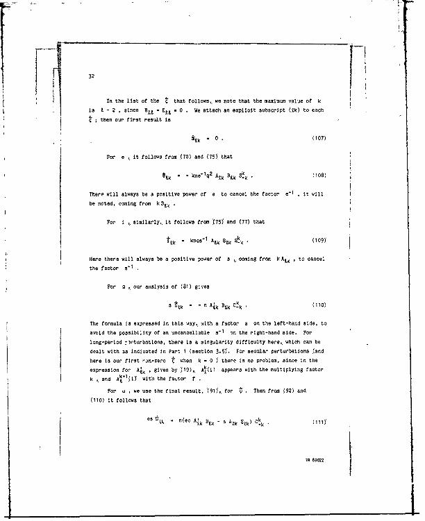
32
In the list of the t that follows, we note that the maximum value of k
Is t - 2 , since B, - Eli , 0. We attach an explicit subscript (1k) to each
then our first result is
*lk " 0 , (107)
For e , it follows from (70) and (75 that
*tk =
kne'lq2 Aik Btk S-k " (108)
There will always be a positive power of e to cancel the factor e-1
, it will
be noted, coming from k Bk
For I , similarly, it follows from (751 and (77) that
t k " knC-1 Ak Bik $% • (109
Here there will always be a positive power of s , coming from kAk ' to cancel
the factor s-1
For 0 , our analysis of (81) gives
3 tk - n A&< Bk C k . (110)
The formula is expressed in this way, with a factor s on the left-hand side, to
avoid the possibility of an uncancellable s-
on the right-hand side. For
long-period rirturbations, there is a singularity difficulty here., which can be
dealt with 3s indicated in Part 1 (section 3.50. For secular perturbations (and
here is our first ran-zero c when k - 0 ) there is no problem, since in the
expression for Aik , given by (19), Ak(i) appears with the multiplying factor
k ,, and A*l(I with the fa tor f
For w , we use the final result, '(910, for Then from (92) and
(110) it follows that
es d - n(ec A k B'k - a A& Elk) Ck b (1110
TR $9022

33
Again the formula is expressed like this to make the right-hand side non-
singular; and again (because Elk contains a factor e when k - 0 as seen
from Table 5) there is no difficulty with secular perturbations.
For M , we combine the results for t and 7 - n' , given by (97), and
(104) respectively; thus
a *1k - nq Alk {Etk - (2t - 1)e B~k} C~k . (112)
From (48), this may also be written as
e * nq3 Aik Bik C~k . (113)
From the definition of L , we may also combine (112) with (91); this gives thenon-esingular result
tk - (21 - 11 nq Auk Bzk C-k . (114)
As usual, a factor e can be cancelled fros both sides of (113) when
k 0 . However, there is a simpler way of dealing with secular perturbations in
M , as indicated in Part 1; Ref 3 was largely devoted to this topic, and the
rest of this section conforms wth the account therein.
The basic idea is that we represent the secular perturbations in mean
anomaly by modifying the value of the mean mean motion. In view of (113), in
fact, we write
IT - n'(1 - e-1q3 I A , (115)
where the summation is now on I , and we have set C0 to unity. This a 'eea
with equation 110 of Ref 3, since At,O here may be identified with
-J Ct(R/p)tAt(i) from that paper.
The logic for using a' a mean semi-major axis (W is, as we have seen,
compelling, so if 1 . n' , we do not retain Kepler's third law in its simplestform. This is of no consequence, however, and we simply write, from 0115),
112X3
u(1 + 2e'lq
3 A O 8 4 (116)
14 89022

K fI34
Ref 3 gives, as equation 15), an explicit version of (116) with (even)
values of t up to 8; the two versions can easily be verified as equivalent if -;
we note that Q, (In Ref 3) is just a normalized form of B',o such that
8ZO - (t - 1)(t - 2)eQ, . (117)
The following recurrence relation was given in Ref 3:
this i. valid for Z. Z , with 02 - 0 and Q3 1 . The relation may be
obtained from 017( and '46). together with
(L - M)t% - 3) B£_, - (L 2)(2Z - 5) BL-2 ,1
- )( - q2 BE.3.1 X119
which derives from 53) on replacing ,(t, J) by (1 - 2, 1).
It is very convenient that Q2 - 0 • It means that for first-order
analysis associated with J2 (the dominant harmonic of the geopotentialO IT is
the same as n' .
6 PERTURBATIONS (SHORT-PERIOD) IN COORDINATES - GENERAL CASE
In this section we develop general expressions for the Or , 6b and Ow
that can be derived from the first-order 68 via the formulae (taken from
section 3.3 of Part 1)
6r - (ra a - (a cos v e -(aeq"1
sin v M ,(120)
6b - (Cos u') 61 - (S sin U') 6n 121)
and
6. - 6,0 (q-2 sin v (I - p/r)) 6e * q-3 (p/r)
2 6M . (122)
Special cases (derived from the choice of integration constants in the 09 are
reserved to section 7, bit in counting the number of terms associated with the
general Ut we have regard to the basis on which these constants are chosen.
TR 89022

35
The 8; are available at once as the v-integrals of the expressions for
d /dv in section 4. Generation of the expressions for Sr and 6w is
essentially straightforward in that the analysis starts with the 6i due to Uk
(which 6i we can denote by 6;tk )' and finishes with 6rtk and Wk . With
b , however, there is a complication, due to the appearance of u' in (121), asopposed to v in (120) and (122); as already noted in section 1, we deal with
the difficulty by deriving 6btx , rather than 6bik .where K has values of
opposite parity to those of k .
We do not give expressions for 6r , ib and 6w , but (as is clear fromPart 11 these are immediately available from tne expressions for r , 6b and
6w , just by replacing Sj and Cj by (respectively! (k - Jj F Cj and
-((k + J) f Sj . We can do better than this if we allow for the (overall) rate of
change of a , replacing (k + j) F by (k + J " + k assuming Cj and $j
still to be shorthand for C- and Sk
6.1 The perturbation ar
We have to apply (120) with 6a Se and 6M given by ',(65) and (the
Integrals of ',(761 and (105). We find that the integrals combine in a very
natural way, as a result of which we can write (with 6r short for 6rik
Sr- (rla) 6a - + a A k I tj {s +k -2 ku<*cj - 2 Ic- "T J, ;< *. ) II
2[k-tZ- I 2k. + t- +c I C *il k +1C .'13[' - kJ- 1.:f * e c I * J k + 2 k(123) II
The simplest way to incorporate (65) is to note that this can be decomposed
intu
dk + 3 -2 V I+tj J-i
2-2 Ic + j 1 -__-e_+ + - ',(124) _
k J- + 1 2 e3 j * j k+ j ] + J) "
By this trick, we can combine '(123) and '(124) at once, to get, say,,
ir - a Atk IStj 1 , ,(125)
TR 89022

36
where Rj (or R~kj to display all the index parameters) is given by
Rj - e(j + I - 1)[l - 2 k 3 J-
+ 2(2j - 2 - Z + 1:J
+ e(j - 0 1)t.- -- 2JC 1 . (126)
It can be seen that (1251 is a sumation in which Rj , as given by 0260,
has three components; each component is expressed as the ss of two multiples ofthe same 'C quantity'. Let us separate the first multiple from the second 'in
each component of Rj ), feeding them back separately into the summation of
(125), so that we have two distinct summations that we can denote by E- and
E. , Thus E- Involves E Btj Rj_ , where
Nj_ - tJ- ----- eCj. 1 * 2 -- C:1 1 3 ~ Z.!e (127)J I+ L 1 j eCj+1
Now we have seen (in section 3) that all sums over B~j can be regarded as
running from -- to - . It follows that we can rearrange the three sets of
terms in EB j Rj. such that (with J now used in a different way)
Z B1j Rj. = (k + j - 1),-1((j I )e Btji 1 + 2(2j + Z - I)Btj
+ 3(J - )e Bt,j1 1ICj (128)
We now invoke the recurrence relation (54) to eliminate B1,j 1 , so that
the quantity In curly brackets in (128) becomes
2(j + t - )BZj + 2(j - i)e Bt,j-
and then simplify further, using (58) with both Z and J reduced by 1, to
reduce this to 2(1 - 1)q2 BLI, j (We get the same result oy using (54) to
eliminate B11.1 first, and then simplifying further via (56)J Thu
Btj Rj. 2( - 1)q2
(k + J - )-i Bt_.j Cj . (129)
TR 89022

3-
Similarly,
B Sj Rj+ - -2(1- 1)q2
(k J 1)-1 BZ..,j Cj. (130)
The final result we require now follows from (125), (129) and (130).
Because of its importance, we write Cj in full. Thus
I
6r1k - - I- ( pAk +(k I )(k +J - 1B1S-1,J cos (ku' - jv) . (131)
Equation (1310 provides a general formula for 6r due to Ut , valid for
I Z I . (This restriction on Z has been operative from the beginning of
section 4.) In view of the fact that k only takes non-negative values of the
same parity as i it should be noted that j takes all values,, but with
BI j only non-zero if 1JI 9 £ - 2 . (This applies if t Z 2 but the case
t - I is trivial because there is an overall factor Z - 1 Y'
If j - - k 1 1 , there is a zero denominator in (1310, and terms with
these values of j must be excluded from the formula; they are associated with
the terms In d;/dv that were hived off in the generation of the t , Insection 7 we shall determine constants for detk and OMRk such that the terms
with these two values of j are forced to zero. It will be noted that all the
cosine terms occurring in (1311, for a given Jt and all possible k , aredi3tinct, except that if k - 0 (1 even) then equal and opposite values of J
lead to identical terms in co3 Jv
We use the remarks in the last paragraph to provide a pair of formulae for
Ntr , the total number of terms required to express Or for a given value of
i . One formula applies when t is odd,, the other when t is even. In both
cases the number of J values for each k (regardless of the excluded values, if
any) is 2 - 3 , if t 2 2
If 1 is odd, there are J(Z - 1) possible values of k , so a priori thevalue of N
Tir is 4(t - 1)(21 - 3) , if I Z 3 . But this must be reduced by
the number of excluded values of the duplet (k, J) . If k - Z , j cannot be
-k ± I , so there is no value to exclude. If k - 1 - 2 ,, J car, (a priori) be-k - 1 and this value must be excluded. If k Z -4 , it will always be
necessary to exclude both -k + I and -k - I . Thus the total number of
exclusions is Z - 2 . Subtracting this from the a-priori value, we get
tR 89022
I

38
NIir . 02_(31. 1) . (132)
Values for t up to 15 (including Nir - 0 , which is the correct value, even
though the above analysis only applies for t 1 3 ) are given in Table 6.
If I is even, there are It - 1 possible values of k , so a priori the
value of NZr is (t + 2)(2 - 3). The exclusions are as recorded before,
amounting to Z - 1 now if k 4 , but it is also naturale for Nir not to
count the 'duplications' that arise when k - 0 ; there are t - 3 of these
duplications if Z 4 , viz for 2 1 iJI t - 2 (we cannot 'discount' for
J{ - 1 , since both values have already been 'excluded'). Thus the total number
of exclusions is effectively increased to 2i - 4 , aid this is the right number
even when Z - 2 (not covered by the argument that applies for Z 4 only).
Subtracting this value from the a-priori value, we get
Ntr - X2 - +(3 - 2) . '133),
Table 6 gives values for Z up to 16. It is remarkable that, as a result of the
discounting of the duplications, we have a formula that is so close to what the
improper use of (132) would give, the value by 0133) being larger by just .
Further,, if we did not discount, the formula for Z 4 , viz Z2 - (t - 4)
would give 1, instead of the correct 2, when X - 2
It is noted, in conclusion, that, due to the multiplier (r/a) of Sa in
(120), it would not be a simple matter to null the 'constant' terms of 6r with
a choice of Z # a' , but that in any case we would prefer not to make such a
choice. Further, the constants in 6a and 6r are not the same, partly due to
the multiplier of 6a referred to, but mainly to the way in which the terms in
Se and 6M combine. For even X , we will have, in particular, a coefficient
of CO (. I) equal to "a - 1)pAL,1 BI, 0 . (See (159 for the constant in da.Y
6.2 The perturbation ab
We get 6b from (121), where 6i and 01 are given by the
integrals of (79) and (82). This is on the assumption that Ob (- 6bk) isassociated with Uk ,, following the decomposition of U, by (5). We shall
shortly find, however, that it is much more convenient to decompose the total
In software in particular, we would rather double a computed quantity than haveto compute it again; in the general analytical formula, (131), however, thereis no easy way to indicate a special situation when k - 0 and j * 0
TR 89022

39
8b (associated with U) as XA6bjw , where the summation Is for values of 1K)
that are of opposite parity to t and we no longer associate the individual 6b
(- 6bt) with specific components of U
In relation to Ut k we get
6b ~ k _ -~ { kc'1 + I '. 1j
The trigonometrical products can be replaced by sums,, in the usual way, and wecan then invoke the notation of (20) to write
Obik " " Bj (k + J),-l(Ai Ck"1
+ A-k Cj+) . (135)
This expression may be contrasted with (125) and (126) for Or . In view of the
difference in superfix, as well as suffix (which alone varied in the terms ofRj 1, in the two C terms of 135), we would now like to combine a pair of terms
with different k indices, before the summation over the J index operates. Wenote that Atk and Aik , though under the summation sign in '135), are actually
independent of J
With the philosophy just referred to, we make the new decomposition
Obi . I 6b K (136)
where each 6b ',(- 6b U is of the form
6b - Tj Bij C" 137)
and we require an expression for Tj (or Ti j to display all the index
parameters). We note first that since '(for non-trivial resultsy k runs from 0or I to t (taking alternate values(, it follows that,, in principle,, K runs
from -1 or 0 to t + I (again alternate values, but of opposite parity to k):for the minimum value of K , only the term in Atk , in (135),; contributes to
Tj , whilst for the maximum value of K , only the term in Aik contributes; for
intermediate values (if any), both terms contribute. But we can straight away
dismiss the 'maximum value' (< - Z - 1), because Att is just a multiple of
at ; from this it follows that AjZ , defined by (20), is zero. (Also Btt - 0
anyway!) We shall find that we do not require the 'minimum value' (K - -1)
either.
TR 89022
...

To evaluate Tj , in general,, we use (30) and '310 for Aik a.d Atk '
respectively. It is fortunate that we require the first with k K - 1 and the
second with k - K + I , since this means that we pick up the same inclination
function, AK(i) ,, for both; moreover, it is aesthetically satisfying to have a
direct application for the inclination functions for which subscript and
superscript ee of opposite parity, as opposed to merely an application in the
propagation of like-parity functions*. We have
it { + 1 (Z - + 1-I + 0,- .(R/P)4 s" Af(i) . (138)T+4( + j - 1)
The quantity in curly brackets in (138) is , pure constant, in which the
aik are given by 12): thus the first a involves P*(O) and the second
Involves P-1(0o), these being given by (13). By relating these to PK,1(0)
we may express the aforesaid quantity (after some algebraic reduction) as
0 t-C*i pC 1(0) f uK,; _ OC.1)
But P ,(O is related to GtK by (16), and thus to AbC by (17). Hence
(138) gives
Tj I Ll_- (139)*T l
The prece4ing is 'general' in that it applies for 1 S K Z Z - 1 (or, more
precisely,, with 2 as lower bound when t is odd); further, if C Z 2 we can
obviouslv cancel the three appearances of u . We still have to cover the cases
< - 0 (1 oddY and K - -1 (1 even,, In which (in princlple only the first term
in curly brackets is to be taken. To count only non-zero terms when Tj is
substituted in (137), the restriction on j is that J I 1- 1 (of an upper
bound of t - 2 in the analysis for r ); we shall be exoluding the values
j C K 1 , of course.
This strengthens the view (noted in other papers, and in section 8 of Ref 13
in particular) that V (of either parity) is a much better index parameter thanKaula's p (where 2p - t - k , referred to iv section 3 here). When theanalysis includes the tesseral harmonics (Ref 9, and see Appendix A here), k
takes negative values (with Akl 1 t ) as well as positive, but the factor ukin (12) is not required.
TR 89022

bhe
When K - 0 , we require just 2/(j 1) from the curly brackets in (139);but for each J > 0 , half this quantity may be combined with half the corres-
ponding quantity for j < 0 , to give /(J + 1), + 1/(-j + 0) , which can be
rewritten as 1/(J + 1) - 1/(J - 1. It follows that (139), with the three
occurrences of u deleted, again gives the right results (counted separately for
j > 0 and j < 0). The modified formula may be seen to apply, finally, for
j-0.
When K - -1 , the position is more complicated. First, the expression by
(139) is not even legitimate now, since At, is not defined for K < 0 ; the
illegitimacy arose in the substitution for Atk , since (310 does not apply when
k - 0 . But (20) indicates that At,O - -Aj,0 ,and this suggests that we can
relate the required term, involving ux+1 with < - -1 . to the te-m in u,_1
when K - 1 . Since C31 - Cjj , the relating will involve the transposition of
positive and negative values of j , and this is also necessary to identify
for K - -1 with u,_I/(c+J-1) for K - 1 . In short, we can
deal with K - -1 just by doubling the second term in curly brackets in (139)
that is associated with K = 1 . This means that, yet again*, we get the "ight
result from e139) if le cancel the three appearances of u
We can now write down the final result we require,; on substituting (1390
into (137) and expressing CK in full. Thus
Sbtu - - I AU, ( * J I)( * J - ) Bj Cos (ul - Jv (lAO)
As already indicated,, this formula is unlike 1310, the corresponding one
for Or , in that it cannot be taken in isolation as relating to a sub-component
of Ut . It is like (1310 in one respect, however, in that terms of OUb£ with
J - I are excluded. In section 7 we shall determine constants for Oik
and 60tk (k . not < , now being the appropriate symbol) such that these terms
are forced to zero.
* The universality of thip procedure (cancelling the u ) stems from theoriginal introduction of UK into the definition of ojK . If we dispensed
with this factor, but used positive values of K as well as negative ones(see also Appendix A), then we would find nothing special about the ialuest1 and 0 in the first place.
TR 8902?

42
We proceed to obtain a pair of formulae for N1b the total number of
terms (without duplication of Cj ) required to express 6b for a given value of
Z Whether t is odd or even, the number of j values for each K (not dis-
counting exoluded values) is 2Z - I , correct for all 1 (9 1) this time.
If Z is even (which we have seen to be the ismpler case), there are 49
possible values of K , so a priori the value of Nib is +L(21 - 1i . When
Z * - I ,, J can be -K I but not -K - I , so there is just one value to
exclude. For all other K , values of K 1 1 are both possible, so the total
number of exclusions is Z - 1 . Subtracting this from the a-priori value, we
get
Nib - 12 - +(01 - 2), . (141)
Interestingly, this is the same as Ntr given by (133). Values for Z up to 16
are given in Table 6.
If t is odd, there are (9. * 0, possible values of K , so a priori the
value of '9b is 4(1 - 1)(21 - 1). There is again a single exclusion if
- I , and two otherwise,, so there are Z basic exclusions (assuming
Z Z 3 ). In addition,, however, there are I - 2 duplications when K - 0 , and
these can be discounted for NIb (though not for 3b itself - see also the
footnote in section 6.1), so the effective number of exclusions is 2Z - 2
this value applies even when k - 1 . Subtracting this total number of
exclusions from the a-priori values we get
N ib - L2 (- i, '(142)
which is one more than for the corresponding N Ir Values for I up to 15 are
given in Table 6.
In conclusion, it is worth remarking that if the planetary equations are
used in Gauss's form, as opposed to Lagrange's, (and this is done in Ref 8), then
the resulting form of the expressions for di and 69 is such as to provide an
easier route to our 6b (With K , rather that k , effectively involved from the
outsetY. For both Or and 6w., however, the approach via Lagrange's form of
IIthe equations is much simpler.
TR e~c2

-43If
6.3 The perturbation 5w
The analysis for 6w is much more like the Ar analysis than the 6b
analysis, because each Uk
can again be treated separately throughout. There
are two complications, however. First, (122) effectively involves cos 2v and
sin 2v , not just cos v and sin v (we see this at equation (143),, following),
and this means that the values j - -k ± 2 are special as well as j - -k ± I
Second, we cannot take Sw to be zero for any of these special cases, since the
constants in 6e and 6M must now be assumed to have been already assigned,
formula for the four special 6w will be obtained in section 7.4. Actually,, a
fifth special case emerges, corresponding to J - -k and a zero denominator
k - J ; 6w for this case can be set to zero, since we still have (for each k)the constant in u ,, as yet unassigned,, available for the purpose - the
constants for AU are determined in section 7.5.
We start by rewriting (122), as
6w - 2q-2
',(e sin v - eq- 1
AM Cos v),
jeq" 2 (e sin 2v + eq-A 6M cos 2v' + + e2q"3
6M + q- 1 6L , (143)
where 6e , 6M and 6L are available from the integrals of (76), (105)' and
(106). The Integrals for 6e and 6M combine in a very natural way and we get
2q-2 '(6e sin v - eq-1 M cos v) +q-2 Alk I 8Bj {e k - -
+3 3. i 2w Z + k 11 : 2k± . I * 2k)S< 3 j )Si-1 + k + J - I k + J + I3S
e3 k 1 k I++ 7}75
jeq- 2
(Ae sin 2v eq"1
AM cos 2v) - J'eq- 2
AU 2 BIJ
13e1-t -k 2 +Z+2k s 1+ t+k+ 1+£- L k
*21 + -2k e - i-k2k +-- j-- 1 -i + +1 + 3e + j 'J+2) ,, (145)
TR $9022

e~q-3 sm 1 + 1- k
T e2q 3 M feq-2 Ak IBsj jea k sj.z2
1-2k +
21 t +2k S 1 +* +k s }146Yk + j
+ k +j--2 SJ+2J
and
4-1 5' - (1 - 20, Aik I B1 - SJr .(147)
We substitute the last four results in (143) and at the same time (as in
tbe analysis for 6r change the interpretation of j so that we can use the
same Si in each term. This leads to
.2 Z + k 211 k I +
L - k),
S4q A& I k j 2 ,- J+
(1 - 2k 6 1e - +k 3 1 + i- 2kk + k + k k+ k +
+ k + -1 , 2 1 + Zi k 1 + +2k2 J+1 + 7+ k + -k+-J
+ 2 4(1 - 2Z + e2(5 - )+ 8 + Z 2k + e2 1 -, - - kik*+J k +J- I k ] - -7 J
2e2 + Z+ k +31 +t,+ 2k +61I - -k + + t-2k]7 +e -+ k + j _ -J-j~
+ 3e211 + X + k +I - Z S '(148)k -e j k + 2 Zj ,J _2 1 j •' I 8
Though the algebra is tedious, we can now eliminate BLJ+2 and 8,J_,
by the appropriate versions of (54). If we express the result as
6w - jq-2 Aik I Vj, 1 B i * Vj, 0 Btj + Vj,.. 1 Bj,j.) Sj ., (149Y
the fo-mulae for Vj,I , Vj,0 and Vj,., are initially very complicated. For
Vj, * in particular,, we start with
3tek'1 k- 4-.2 + 6(4-1.1+12e ( 1)(k +'J 72) k +j +2 k +J + I3( - -) 3k 2(k41-1)}
(j +z +1 )(k . J) k+J ' k I-
TR 89022reaso Ii
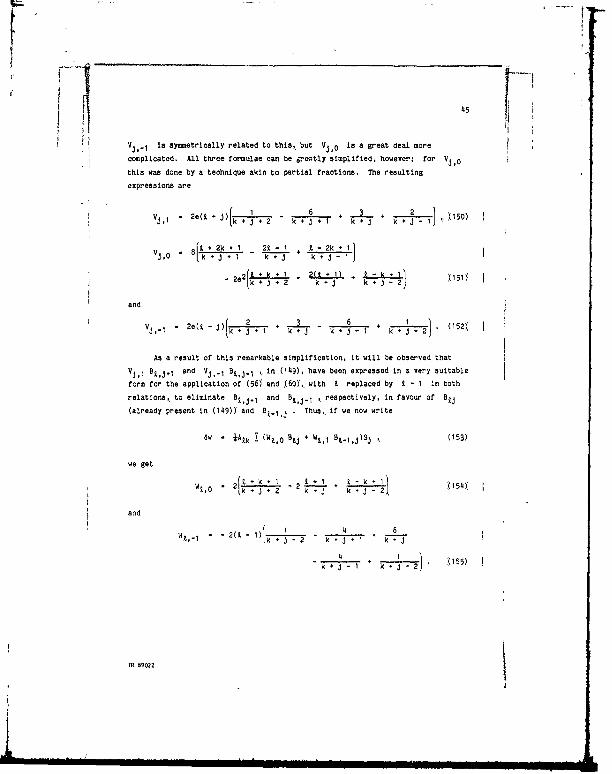
H 45Vj,._ is symmetrically related to this, but Vj 0 is a great deal more
complicated. All three formulae can be greatly simplified, however; for VJ,0
this was done by a technique akin to partial fractions. The resulting
expressions are
Vj, - 2e( ) +J 2 k 6 3 2
k + + I - k j - 150)
8ft +2k +1 U 1.. + } 2
2 k _ -2 k.J 1512
and
Wt- 2e(-J) 2 + . j-1 k- J (152
As a result of this remarkable simplification, it will be observed that
V ,1 Btj I and Vj,.I Bz,j.i ,, in (149), have been expressed in a very suitable
form for the application of (56)' and (60, with Z replaced by t - I In both
relations,, to eliminate Btj+I and B *,j. , respectively, in favour of Bj
(already present in (149))' and B,.I,j . Thus, if we now write
6w - +Atk I (Wto ati + W1 , I t.;I,j)Sj . (153)
we get
W,' - 2[;' 1+ -k; 2----- - k+(154),t, kv * k. + +*J- 2 J
and
W£,_I + - ( ) J 2 Tr J+ 1 + k J
4 + 1 - (155)kv+j- k+7-
TR $9022

46
The final result we require follows from the substitution of (154) and
(155) into (153). Writing Sj in full, we get
(1 k) into (1)1 [(2(1 0 - k(k l w)e BteaWik " Atk 77-( -J 2)(k k j)(k + J - 2)k6()" 1+ B sin (ul + JvY . (156)
7(k+- j !4 l)( j i- I) BZ- J '
Equation (156) is the general formula for 6w due to U As with 131)
and (140), for 6r and Ob respectively, it applies for all t 1 like
'( 40) but unlike (131), on the other hand, values of Ili up to t 1 are
required to cover all the non-zero terms. For each k , zero denominators exist
for five different values of j : for four of these values ( J - -k ± I and
J - -k a 2 ), special formulae are required, in place of (156), as already noted;
only for the fifth value C J -k can a term (for each k C be actually
excluded.
Before proceeding to a poir of formulae for NUw , the total number of
terms required to express 6w for a given value of i , we note (and make
allowance for) one specific null term that arises for each even value of L
For k - 2 and j - t - I , we see from (156) that the coefficient of Btj is
identically zero (i.e. independently of i Y. But BtI,j is itself zero when
j - I - 1 ,, so this -pecific term of 6wi,2 always vanishes. Proceiding to
NMw , we first note that the number of J values for each k (regardless of any
exclusionY is 2Z - 1 (for all L 1 1 C.
If t is odd, then a priori the value of Nw is +(Z )(2 - 1.
There is one excluded value of j for each k - Z , so there are J(t - 1)
exclusions altogether. It follows that
N5w - b
2 , (157)
and values for Z up to 15 are given in Table 6.
If L is even, the a-priori value of Niw is +( + 2)(21 - 1) . There is
again an excluded j for each k * t . amounting to +Z basic exclusions, but
there are now two other sources of discounted re~mz. We have just remarked on
the particular zero term that arises for k - 2 ; wa might prefer to allow zero
actually to be computed in a general computer progran, but here we regard this
TR e9022

147
term as an exclusion. The other source of discounted terms consists of the
t - I duplications that occur when k 0 (see the footnote of section 6.1 .
Thus the number of effective exclusions is + , and from subtraction we obtain
2 - 1 . (158)
Values for Z up to 16 are give in Table 6.
6.4 Universality of results (non-elliptic orbits)
Equations (1310, (1'0) and (156) give, on summing over k or K as
appropriate,, general formulae for the perturbations dr , 6b and 6w
respectively, due to U . It is being tacitly assumed, in the rest of the
Report, that we are only considering elliptic orbits. It is worth remarking
here,; therefore, that (as follows by a continuity argument) the formulae are also
valid for parabolic and hyperbolic orbits. The formulae are effectively
universal14, in other words, though they inevitably fail for rectilinear orbits
'(with infinities arising from zero p).
7 THE SPECIAL CASES, AND INTEGRATION CONSTANTS
The main results in this section,; obtained in section 7.4, are the formulae
required to supplement (156), the general formula for 6w . These formulae,
covering the cases j - -k ± 1 and -k 1 2 ,, are forced by the 'constants' for
6e and 6M , which are determined so that certain terms (those for j - -k ± 1Y
can be excluded from 6r . Though we have omitted (in section 4J the full
expressions for the short-period perturbations, 6 , in the elements,, we give
here the adopted 'constants' for all the . Five of the elements have
constants chosen to suit 6r , 6b and 6w for completeness, we start with
the lemi-major axis, for which the constants are mandated by the use of a'
as5 .
7.1 Mandatory constants for 6a
We go back to the original expression for 6a due to UZ , vim (63). We
can expand the conplete factor )p/r)t1+
in terms of the Bt.2,j (ocf the
expansion via the Bfj in (65)). On taking just the term of the expansion with
j - -k , we isolate the constant term that (for each k * and a given J. is
mandated by taking S a'
TR 89022
li ii i I,- .. . l -
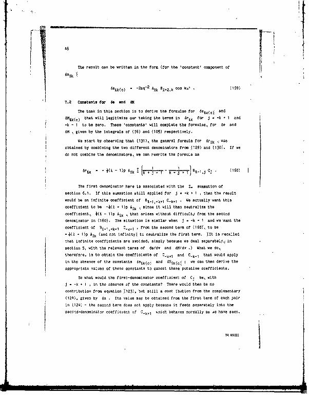
48
The result can be written in the form (for the 'constant' component of
6aik(c) " -2aq-2
A~k BL 2,k Cos k'. (159)
7.2 Constants for 6e and 6M
The task in this section is to derive the formulae for detk(OY an
amik(c) that will legitimize our taking the terms in 6rik for j - -k - 1 and
-k -I to be zero. These 'constants' will complete the formulae, for 6e and
6M , given by the integrals of (76) and (105) respectively.
We start by observing that (131)a the general formula for 6rmk 1 was
obtained by combining the two different denominators from 129Y and (30). If we
do not combine the denominators, we can rewrite the formula as
-1ink -Au ( *~ 1 B Z ~~-1.j Cj . (160)r~k - - +(X - 1)p A & I ( + - k + j + 1)B ' , C 1 0
The first denominator here is associated with the E. summation of
section 6.1. If this summation still applied for j - -k +1 , then the result
would be an infinite coefficient of B.1..k+1 C-k+l . We actually want this
coefficient to be -(t - 1)p Ak 1, since it will then neutralize the
coefficient, 4(i - 1)p Atk , that arises without difficulty from the second
denominator in (160). The situation is similar when j - -k - I and we want the
coefficient of Bt.l,.k.1 C_k.l . from the second term of (160, to be
- (Z - 1Ip Aik (and not infinity) tco neutralize the first term. '(It is recalled
that infinite coefficients are avoided, simply because we deal separately,, in
section 5, with the relevant terms of de/dv and dM/dv .) What we do,therefore, is to obtain the coefficients of C~k I and C-k-1 that would apply
in the absence of the constants e ( ) and 6Mtk(c( ; we can then derive the
appropriate values of these constants to cancel these putative coefficients.
So what would the first-denominator coefficient of Cj be, with
J - -k + I , in the absence of the constants? There would then be no
contribution from equation 0(23). but still a cont tibution from the complementary
(124), given by 6a . Its value may be obtained from the first term of each pair
in (124) - the second term does not apply because it feeds separately into the
second-denominator coefficient of C_k+1 which behaves normally as we have seen.
TR 89022

49
But equation (124) was written down before the 'rearrangement', from (127)
to (128), in which the use of J changed. This change affects the B subscripts,
and it may be seen that the required first-denominator coefficient of Ck+1 in
- a AUk (eBj,~k+2 + 4BZ,.k, 1 + 3eBk-k ) .
The (normally behaved) second-denominator coefficient, on the other hand,,
may be written
Sakk(I - 1 q2 B l.+
To cancel the combined coefficient by use of 6etk(0c and 6M~k(C),
let us suppose that
6elk(c) - Atk x C.k (161)
and
Smtk(c - AU1 e-1 q y S-k, (162)'
where x and y are quantities to be determined. On combining these for a
contribution to 6r '(cf 120)), we get a coefficient of C.k+1 given by
- 4 a A1k (x * y)
so that one equation to be satisfied by x and y is
2(x + y) + eB, k+2 -4BZ.k+l + 3eBt,. - - 1) q2 Bt.1 k l - 0 . '163)
The complementary contribution to 6r from (1610 and (162) leads to a term in
Ck I ,. of coefficient
- 4a Ak (x y),
and this combines with two other coefficients of C_k 1 ,, obtained as in the last
paragraph; the result is another equation in x and y
2(x - y) - eBt,_k_2 + 4B ,.k.11 + 3eBi,.k - (t - 1) q2 BZ.IM.I. 0 . (164)
TR 89022 I

Souto of (163) and '(164) gives
x - +{(L - 1)q2 (B1 -l,-kal
+ Bi-1,-k-l " 6eBt,-k
LT - ~4(Bt,_k~l + B£,kl - e(B£,k+ B ,_2) 0165Y
and
y - {(1 - 1)q2
(B1.l. 1 k l -l,1 )
- J;(BZ,_k+1 - BZ,_k_1 - e(B_,-k+2 i,-k-2)} (166)
To get the formulae for 6etk(c) and 6Htk(c) that we require, it remains to
substitute (165) and (166) into (161) and (162). In doing this, we make two
simplifications; we eliminate Bt._,k+I and B.. 1. 1 by use of (60) and
(56), respectively (with t replaced by t - 1 in each case); and we write
BX,k etc rather than Bt,_k
Finally, then,, we have
6etk(C) - - + A11 {eBt,k 2 - CZ + k - 4)Bi,k I + 2(t + 2)eBtk
- (I - k - 4)Bt,k.I + eBZ,k. 21 cos kW' C167)
and
d1k(c) - e
- 1 q Ak JeB 1,+ 2 ',(t - k - 4)Bt,k I
- 2keB1k -*t - k - 4)BZ,k.1 - et,k. 2 ] sin kw' . (168)
The formulae could, of course, be reduced to a smaller number of terms, by use of
the fixed-Z recurrence relation, C54), but the coefficients would then be much
more awkward; no genuinely simpler versions of (167C and (168) have been found.
7.3 Constants for 61 and 69
In this section we derIve formulae for 6itk(c) and 'Olk(cY to
legitimize our taking the terms for J - -K - 1 and -K - I in '(140), the
general expression for 6b1( , to be zero. The analysis is sonewhat simpler than
that in the preceding section, in spite of the complexity entailed by 'he need to
work with both k and
TR 8902

51
As with 6rt ,, we start by observing that (140) was obtained by combining
two denominators, which appear separately in the preceding (139). When
j - -K * 1 , the second denominator becomes zero and no longer operates; from
the first alone we get, as the effective term in (140), it A. BZ ,+I CfC
When j - -K - 1 , similarly, the first denominator in (139) does not operate,
and (140) effectively reduces to +t AU Bt,-K-1 C K 1 These terms have to be
cancelled by the use of 6iik(c( and 6tk(c) , with appropriate k , so we
suppose that
Sitk(c x C-k '(160)
and
6A(o) -1
Y S170)
(In the last section we were able to include Aik in the corresponding
expressions, 1611 and (162), but there is no common factor available now.) On
combining (169) and (170) for a contribution to 6b (of '(121),, we get
+(x - y, Ck1
- +(x + y ck -i
If we postpone consideration of any difficulties associated with the
extreme values of k that arise,: then we get a pair of equations for x and y
on identifying g with k * I and k - 1 , respectively, in the coefficients of
and C 1 that have been recorded. Thus the equations are
2(x - yY * t At,k 1 g,-k - 0 (171)
and
2(x + y + t A,k.I Bi,.-k - 0 . 172)
Solution gives
x - tCAZ,k, + At,k 1)B,.e '(173)
and
Y -90A,k+ AZ,k_1)B,. k . 174)
TR 89022

52
The expressions in brackets can be replaced by simpler expreaalona, following
(27) and (28), and we also replace Bt,.k by Bik * Then substitution in (169) iand (170) gives us the formulae we require. Thus
Sitk(c) - BAk B cos k.' (175)
and
k(o) kcs"2 k sin k, (176)
We now have to show that (175) and (176) are valid for the extreme values
of k as well as 'general values'. For k - 9 , the maximum value of k , there
is no difficulty (171) involves a value of Z * I for K in 8b , but this is
all right as B - 0 cf section 6.2); thus x - y - 0 for k - L . For the
minimum value of k (0 or 1, according to whether t is even or odd), it is a
little more complicated: we consider the two cases separately.
If Z is even, with k - 0 , C1 and C61 are the same and we cannot
Separate x y from x - y in the combination of (169) and (170). Thus there
is only one equation to be satisfied (instead of both (1710 and (172) , and it
involves only the identification of K with k + 1 (not also with k - I (.
The equation reduces to
x - -44 A1 ,1 8 ,0 (177),
which is consistent with (175), in view of (29) The value of y is
indeterminate, but this is appropriate for the coefficient of sin kw' , which is
itself zero when k - 0 . If t is odd (with k - I ), on the otl-r hand, the
validity of (175) and (176), follows in essence from the argument just prior to
the establishment of equation (lO), and the details are omitted.
A last point in this section is noted as no more than a cariosity. Whereas
the rest of 8ilk and 6nik contain Aik and A& , respectively, as a factor
of every term,, as indicated by (79 and (82), these factors are reversed in the
'constant' terms,, as indicated by '175Y and '076). The point was noted, for
t 3, in Part I.
ne 89022 I.,iI !+I

'53
7.4 Forced terms in 6w
We now have, for each U only one 'constant' at our disposal; denoted by
dutk(c) , it will be determined in section 7.5 so as to validate the nulling of
the ter-a for j - -k in the formula, (156), for 6wik . For J - -k ± I and
-k 1 2 , on the other' hand, we are forced to accept non-null terms that arise,
via (122), from (167) and (168), the formulae for 6eik(c) and 6'ik(c) . We
derive the formulae for these terms in the present section, which must therefore
be regarded (from the reference viewpoint) as a completion of section 6.
For each of the four special values of j , in principle we embark on a
procedure that is similar to that employed in section 7.2. The basis of this
procedure is that we re-determine the expression for 6w with the appropriate
terms in 6e and 6M (which in their general form would lead to infinities)
replaced by 'constants' proportional to x and y (as defired by (16) and
(162)); the only difference (in principle) from section 7.2 is that we do not
have unknowns to solve for, so that the procedure is 'direct'. In practice,
however, because the basic formula for 6w ,. (122), is so much more complicated
than the corresponding formula for 6r , (120), it is better to proceed a little
differently from this: instead of developing our four special formulae more or
less ab initio, we start four times from the (final) general formula for aw
156), and modify it each time in the appropriate manner.
We start with j - -k - I ; it will be useful to have a shorthand for the
denominator that becomes Zero, so we define
d - k * J - 1 '(178)
for general j and will eventually set d - 0 . In terms of d ,. we can rewrite
,(54) and (155), which on substitution into '(153)' give the final (156), as
i k* 1, 2['1 < - k 1di, + I* d 2I. - (179)
and
4i 6 4 +-.LA '10Idi +2t) ld3 d +2 d +1 d d-1I
* I.. .I
* R $9022
muuu~2 LA
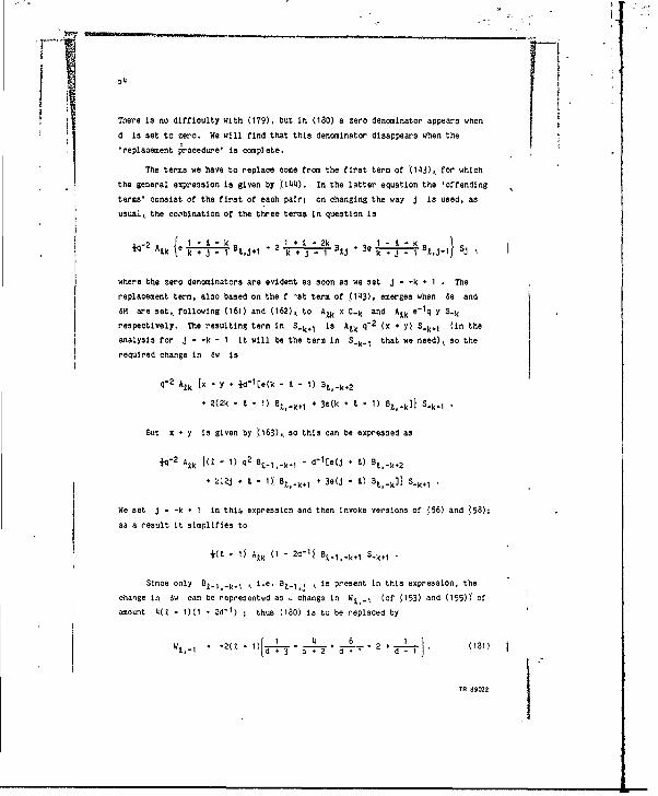
t,
There is no difficulty with (179), but In (180) a zero denominator appears when Fd Is set to zero. We will find that this denominator disappears when the'replacement procedure' 13 complete.
The terms we have to replace omie from the first term of ,(143), for which
the general expression is given by (1I44). In the latter equation the 'offending
terms' consist Of the first of each pair; on changing the way j is used, as
usual, the co'bination of the three terms in question Is
*1-2 {~ e 1 + 1 BZ,j+. +2; t 2 Btj + e1 Bt,J.;} SjA k + j 3e k + ~ -1 -'-k
where the zero denominators are evident a3 soon as we set ,j -k + 1 . The
replacement term, aloo based on the f 'at term of 04A3), emerges when 6e and
6M are set, following (160 and (162), to Al x C..k and Atk e-q IQY S-krespectively. The resulting term in -k is AZX q-
2 (x - y), S-- (in the
analysis for a - -k- I it will be the term in Sk-1 that we need), so the
required change in 4w is
q-2 At (x +y ++d
1'O(k - Zi-I1) BEk.2
+2(2k - Z - 1) St-+ + 3e(k - Z - 1) Bi..k)} S..i,;
But x + y is given by '(163), so this can be expressed as
jq'2 ilk I" - 1) q
2 Btl k- - d-ie(j + t) Bl--
+ 2ae - Z - 0, Bt-~ + 3eQi - Z) Bt,..i)I S..k,;
We set a - -k - 1 In this expression and then invoke versions of (56) and (58);
s a result it simplifies to
+t- 10 Alk (I - 2d1Y Bt.1 -kl S-k+1
Since only Bt;.,-k; ,, i.e, Bt_.;j ,~ is present in this expression, the
change In 6w can be represented as .change in WZ1 1 (of (153) and (155)Y of
amount 4(Z - 1 2d1) ;than (180) is to be replaced by
1 14 + 6 +
ye 49022

55
It is now legitimate to set d - 0 in (179) and (181), the result being
It, 0 -(2- k 2)
and
Wz,-. -4(t - 10
On substituting in (153). we get the first of our four special formulae; it can
be written (with a change of sign in the second suffix of each B
wtk,_ - - Atk{(2Z - k - 2) Bi,k.1
(z - 1) B 1 . 1 }1 sin (kw' + v( . (182)
The second special case is with j - -k - I . This is the twin of the
first case, so it involves
d - k + 1 (183)
and the expression for x - y given by '(164). There is no point in a virtual
repetition of the analysis in detail, so we proceed direct to our second special
formula; it can be written
6w k,-k-1 - + Atk(2t - < + 2' Bk 1
+ 'a - 1) B 1. sin (k.' - v) . '(184)
The symmetry between 182Y and (184) is obvious. For k - 0 , of course, the
equations reduce to the same formula, and the footnote of section 6.1 is again
relevant.
For our third special case, we require to set j - -k * 2 , so we start by
defining
d - k + J - 2 . 185)
Then (154) and (155) take the form
Wa,0 - 2 1 k I - 2 .-'.- . d) (186)
TR 89022

56
and
W6 4Z.1- -2(t - 1), d 3 d +2 d+ 1 d 087),
with the potentially zero denominator In both expressions.
The terms of the general (156) that we have to replace now cate from the
second term of (143), for which the general expression is given by 0(I45). The
'offending terms' are the last three of the six that occur in the latter
equation; with the usual re-interpretation of j , these three terms In
combination give
eq. 2 AU {e + - 2 k B 1 -2k B,
k ~ + j 2 k -j 2 + j Z,-2 sj
The replacement term in now Alk eq"2
(x y), S.k+2 , no the required change in
eq"2
A9. Ix - y - d-l[e(k - Z - 1)at,.k. 2
+ 2(2k - Z - 1) eZ,.k+1 - 3e(k . - 1) BE.k]) S-.k,2
With x + y given by '(163)., this can be expressed as
+ eq" 2
Atk {(J - 1)q2
Btl-.k+l - d-1[e(J + 9 -)Bt k-2
+ 2(2 + I - 3)Bt..k. I + 3e(Q - Z - 1)B,.kl S-k 2
We set j - -k + 2 in this expression and then Invoke versions of (514),
,(57) and ,5 ) to eliminate Bt.I._k+ I . BZ,k+I and in favour of
Bt-,-k+2. Thin simplifies the result (for the change) to
- + AiR(2d'i I)(t - k + I + d)Bt, _k+ -k (9 - 1)R.1,-k+2} S-k+2
It now follows, from 816) and 187), that the altered values of WR,0 and
W%._* to be substituted in (153),, are given by
2, [' - 2 +) (X - k - 1 + d) (188)
TR 89022

F57and 10
W -, 01 ' ( (19)
and
Wt,.I -( 1)(1I . (189)
Wk'-1 -U 19
Thus the substitution gives, for our third formula,
6wtk,-k-2 - " Ak {3( + k ' 5)8tk-2 - 19(1 - 1)B_1,k.2}sLn (kw' + 2v) .
...(192)
Our final special case,, with J - -k - 2 , is the twin of the preceding
(third) case and involves
d k J + 2 193)
We will not go through the analysis in detail, in view of the symmetry, but
proceed directly to the final formula; it is
6wtk,.k.2 " Ak 13(t - k + 5)Bt,k+ 2 - 19(t - 1)B_1,2 } sin (kw' - 2v)
...(194)
7.5 Constants for dw
To complete section 7, it remains to determine the constant, 6Owk(o
that legitimizes our taking the term for j - -k In (156), the general
expression for 6wik 1, to be zero. We already have 6Mk(c) , given by (168), 30
we only need to determine RLik(c) , the constant in 6ILk , for 6wtk(0 to be
known at once.
TR 89022

58
We start by now defining
d k j (195)
so that (154) and (155), in their general form with potentially zero
denominators, are rewritten as
d-22 - +1+1 (196)
and
(1 4 6 4 + I07Wt',1 - 2(t - 1) +
1+ 2 d + I d d-1 I d 197
The zero denominators will disappear when, for the coefficient of S-k in (153),we replace a quantity occurring in the general analysis with a quantity based onaMtk(c) '(6e1k(c) not being involved); then 6ILtk(c)' is defined to null this
resulting coeffiolent.
The quantity to be replaced derives from the combination of (146) and(147). With our usual re-interpretation of j , we can write the resulting
coefficient of S-k as the sum of
Seq " 2 Atk d
- 1 e(1 - kBt,j 2 - 2(1 + Z - 2k)BOtj~l
*6e(I - +t)Bj + 2(1 + Z - 2k)Bt,j.; I e(1 + Z - k)BZ.J_2*
andS(1- 20( At, d
1 Bij
associated with I e2 q-
3 6M and q-1 6L respectively. The quantity that has
to replace this coefficient is available immediately from (168), but it is moreconvenient to back-track a little and take it instead as + eq"2 AU, y , with ygiven by (166). Thus the replacement coefficient may be written,, with J rather
than -k in the B subscripts, as
- eq"2 Alk le BAj 2 + 4 B1,j+ - e , - ,j2 Tnupef
"1 " (
" ~~~~1 1q 2 (BL-, J-,-l
TR $9022

q2
I)~j,2 ~ j*59
On subtracting from this the coefficient being replaced, we get
, T Atk q2d-1
{3e2(t j - I *tj+ 6e(9. + 2j + 1)B
-2Ei4(21 -11 + e2(t - DI + 6ei - 2j 1 jj
+ 3e2(t - j1 + I)B Z,J.2 - 39q
2 d(Z - 1)BZ-j,j~i - tJ0
By application of versions of the five relations (541) to (58), we can eliminate
Bt,+ and t1,J2 ,then B1t,i and Bt _ and finally BZ1.. 1 and
at1'- - This reduces the foregoing expression to
+A11 d'(E[2(1 - 1 - 3jd) Btj + 6(1 - l)Bti ii
which represents (when j - -k the adjustment required to the coefficient of
S..1 In dw . On adding the appropriate contributions to (196Y, and (197) we get
W (t+k. + I 1I- k . 1 3j1181.0 d -2 d -2 -3jii
and
, + 2 d.I d-1 d-2
We can now set d - 0 (i.e. J1 - -k Y, getting
WE0 - 8k (200)
W .- -0. (201)
ad These results mean that, in the absence of 6Ltk(C) . we would have
k Aik<Bt4 a the coefficient of S-k~ In d 1k so, to null this, we take
6114(0 k q AU Blk sin ko' Q2)
TR 5902i
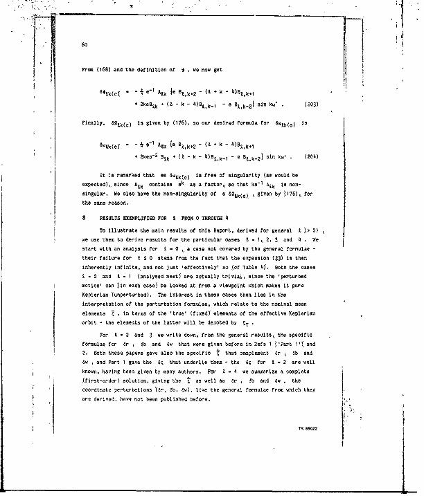
60
From (168) and the definition of ,we now get
e- - e1
Ak [a et,k+2 - (t - k - 4)B,k+1
+ 2keBtk + (I -k - 4)Bt,k_1 - e Bt,k_21 sin AW' . (203)
Finally, 601k(e) is given by (176), so our desired formula for Swtk(o is
Wt(Oc - - 1 e ALA (a g9,k+2 - (9 + k - 4)Bt,k+ I
+ 2kes-2
Btk + (Z - k - 4)Bt,k.1 - e Bt,k.2} sin kw' . (204)
It is remarked that as 6wik(c) is free of singularity (as would be
expected), since Atk contains 3k as a factor,, so that ks"
A9 k is non-
singular. We also have the non-singularity of a 60tk(c) ,, given by '176), for
the same reason.
8 RESULTS EXEMPLIFIED FOR L FROM 0 THROUGH 4
To illustrate the main results of this Report, derived for general 1 > 0)
we use them to derive results for the particular cases Z I,, 2, 3 and 4 We
start with an analysis for Z - 0 ,. a case not covered by the general formulae -
their failure for t 6 0 stems from the fact that the expansion (33) is then
Inherently infinite,, and not just 'effectively' so (cf Table 0i. Both the cases
t - 0 and t - I (analysed next are actually trivial, since the 'perturbed
motion' can (in each caseY be looked at from a viewpoint which makes it pure
Keplerian 'unperturbed). The interest in these cases then lies in the
interpretation of the perturbation formulae, which relate to the nominal mean
elements Z , in terms of the 'true' (fixed elements of the effective Keplerian
orbit - the elements of the latter will be denoted by T '
For t - 2 and 3 we write down,, from the general results,, the specific
formulae for dr , 6b and 6w that were given before in Refs I ('Part 1'), and
2. Both these papers gave also the specific ' that complement 6r ,. 6b and6w , and Part I gave the 64 that underlie them -the 6 for Z - 2 are well
known. having been given by many authors. For Z -4 we summarize a complete
(first-order) solution, giving the ' as well as 6r , 6b and 6w , the
coordinate perturbations '(6r, 6b, 6w), like the general formulae from which they
are derived, have not been published before.
TR e9022

61
8.1 The trivial (but exceptional) case 1 - 0
From (4), we have
U0 - - Jo . (205)
This is confirmed by (15), in which k is restricted to zero so that U0 U;
am 0 and A( are both unity, so AO o by (). Thus the effect of
Jo is to reduce the power of the central force as indicated In Ref 4. the valueof the overall 'true' power being given by
uT I ( - JO)
.(206)
The orbit can be fully represented by UT and the 'true elements' T
but it is instructive to exhibit the behaviour of the osculating elements , as
well as the perturbations Sr , 6b and 6w ) relative to the u originallyass.umed. As the general results of the paper do not apply when Z - 0 , it Is
simplest to derive formulae from the original planetary equations directly.
There are no out-of-plane effects, even as a 'trivial' phenomenon, since we at
once get
61 - 60 - 6b 0 '(207),
so that
- IT and 1 - OT (208)
From (62) and (205) it follows that
6a - a - a' - -2J0a2/r (209)
This is a flirst-order relation, as usual, with a on the right-hand side
interpreted as a' (- X Y; it becomes exact if a2
Is interpreted as aa'There should be no surprise that (osculating) a varlec around the orbit (unless
it is circular)i this results from the use of the 'wrong' u ; with the 'right'
U (uT). the osculating a would have the fixed value aT . Since with rT r
TR 8921
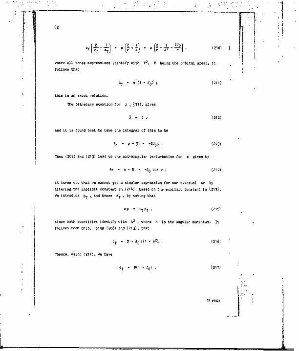
62 'T- -L
O) " - (210)
where all three expressions identify with V2, V being the orbital speed, it
follows that
aT - a'(1 - Jo (2110
this is an exaot 'elation.
The planetary equation for p ,, ,(70, gives
p - 0(12
and it is found best to take the integral ot this to be
ap - p - V - -2Joa . (213)
Then (209) and (213) lead to the non-singular perturbation for e given by
Se = e - T - -Jo 003 V (214
it turns out that we cannot get a simpler expression for our eventual ar by
altering the implicit constant in (214), based on the explicit constant in '(213Y.
We introduce PT , and hence eT , by noting that
VP - PTPT 1 (215)
since both quantities identify witn h2 , where h is the angular momentum. It
follows from this, using ,(206) and (213). that
pT " 1- Joa(1 - e2) . (216)
Thence, using (211), we have
eT - + J(o) . (217)
TR 89022

r 11,
63
t The planetary equation for * , (83), leads to
dv 0 J e1
cos v, (218)
and we take the integral of this to be
- - = Jo e-1
sin v , (219Y
since (it turns out we cannot get a simpler expression for dw by changing the
(implicit) constant. Hence also
6wu- u- - -Jo e-1
sin v .(2201
We introduce WT via vT . noting that (6), taken with and without T-suffixes
(and with rT - r ), yields
'(P - PT)/r (e - eT cos v - e(v - vT( sin v .(221)
This leads to
v - vT - Jo e-1
sin v '(222)
and hence (taking u - uT)
- a T - - e'l sin v . (223)
From (220), we now see that
r , • (224)
The planetary equation for p , (93), leads to
d 2Jo q r/p , '(225)Tdv
TR 89022

-6
and this introduces a difficulty in the analysis for M since (for the first
time) we effectively have a negative power of I + e cos v . The simplest way to
deal with the situation is to change the integra.ion variable* from true anomaly,
v , to eccentric anomaly, E . Instead of (225), we have
-2 0 ;(226)
the integral of this is evidently secular, rather than short-periodic, but for
convenience we use the notation appropriate to short-period perturbations and
write (with the most useful integration constant)
6p - -2J0E . (227)
Toe secular perturbation in p , that has just emerged, is dealt with in
the usual way by choice of a suitable value for I ., not compelled to be equal to
'I ' . With
nT2 aT3 - - Jo* '(228)
we naturally take
1 - nT , nl/(1 - Joy (229)
exactly, the formula being compatible with (211). (Equation '229) is in the
spirit of '115), though not just a particular case of the earlier equation, which
is only valid for Z > 0 . Then (209) and (229) give
df
dT n - TT + J.n(3a/r - 1 .(230)
and hence
$ - Tit . JO 3E - H) '(231)
* The use of E as integration variable leads to a (finite) solution of thegeneral problem when Z < 0 . The analysis is more complicated now, however,,as v has to be replaced by E in occurrences of sin u , induced by thefactor P-Z-I (in y) of UX , as well as in the basic (negative) power of1 + e cos v that arises.
TR 89022

65
In combination with (227) we may now write
6 - Jo (E - M) = Joe sin E (232)
(using Kepler's equationY. Using (219), we finally get
am - M - Joe-1
(q sin v * e2
sin E) (233)
We introduce MT via ET , since from the equation
r - a(i - e cos E) (234)
we get (with r -rT ,and both a- aT and e - eT known)
E - ET = Joe-1q-
1 sin v (235)
Then subtraction of the versions of Kepler's equation for M and MT , with the
aid of e - eT again, leads to
M - mT - Joe -1
'q sin v + e2 sin E) , (236)
so that (233) yields
MT - '(237)
Thus four of the 4T are the same as the corresponding , the only
differences being for the elements a and e Further, we can apply (120) and
(122) to the i , getting
6r Joa(e2q-1 sin v sin E - 1) (238)
and
6w - Joeq2 sin v '2 - e cos v) .239)
In view of )207,. this completes the analysis for t - 0
TR 022

U1~ UJ R siJ~ in 8 (240),
r2
This transforms t,)
U 1 V I-PL.Cos U' '(241)
by (15), In the general analysis, where
A1 J~ , a 242)
by 01), and sin B-s sinu -aco,;u' As noted in Ref 4, '(240) implies that
P , , V& -z - rz cs (4w O~12(243(r U ~r r o + )~*0d2
where Z - -Jj R so3 the overall potential is th, same '(to first order(, as :or acentral force towards the point at distance z ,,and axially 'north', fron the
nominal centre of 'unperturbed' attraction. (The precise representation of this
configuration requires that for each t > 0 ,, JE has a specific value, given by
..(..4 )i -)
Wle have three essentially equivalent parometer3 ( J1 , AlI and z (, and
our formulae can be expressed in terms of any one of these, but it is more
convenient to use a fourth parameter, X. , defined by
A c Zp - -3 1 AlI - -Jj a/p '(244)
Then the general formulae, taken with Z I , lead to the followingt (131)
gives
6r -0 '(245)
(1040). with < 0 and J -0 ,gives
6b - On '(246)
Ta 89022

67
and (182), with k - 1 * gives
6w - - sos u. (247),
Though (247) is taken from a special-case formula (because J -k 1 1 , the
general formula, 156), actually gives the same result because the second term of
this formula, which is responsible for the zero denominator, does not arise. Our
formulae are consistent with (132),, (142) and (157), which give
(Nl,r, N1,b, NI,w ) - (0, 1, 11 ,(248)
as seen also from Table 6.
Expressions for the 6C can be written down easily enough,, following the
general analysis, but it is of more interest to obtain formulae relating the
(mean elements relative to the nominal attraction centre to the ;T 'unchanging
osculating elements relative to the 'true' centreY. This can be done via the
)verying osculating elements) and derived quantities, since no conventional
definitions are involved in relating the C to the T •
We start with '(243), which may be taken to express V/rT . It leads to
r - rT - Ap sin B , (249)
so that,, in view of (245),
- rT + Aps sin u .(250)
Now this is true for all u ; but I- aT , T - eT and R -MT must all be
independent of u , whilst defining I - rT via (120). This is only possible if
- a, (251)
- eT - 1q2s sin (252)
and
M, A * e-q3
s cos w (253)
r 90228

68
Thus we have established three of the desired relationships; (251) could
also be obtained, more directly, by identifying two different expressions for V2
(of (210)).
We can proceed in a similar way to get the relationships for I and a
Some geometrical visualization is neede', and we may regard the difeerence
between b and bT as validly defined, independently of the precise location of
the 'mean orbital plane' which is involved in defining the coordinate b . This
difference is given by a projection of the displacement z perpendicular to the
(meanl orbital l.lane, such that
b - bT - cz/r - Xcp/r . (254)
Then from '(2466,
Sb T - ce cos v (255)
(where U is actually zero, by definition, but this is not relevant to the
argument). AS with (250), this is true for all u , whilst V - bT may be
expresed in terms of T - iT and T - T via (121 . It follows that
T i T Ace sin w (256)
and
i OT - Ics-le Cos w . (257)
This only leaves the relationship between 7 and w to be established.
It was not obvious how to proceed, analogously to (249) and (254), via a formula
for w - wT , so the procedure adopted was based on formulae for V - vT and
- uT . The first of these comes easily from (252) and (253); thus
V - vT
a +ie-'s {e2 cos (u - v) - 4e cos u - (2 - e
2) cos .) . (258)
For the other relationship, we need the special formula (that can be derived for
the given geometry)
c(u - uT ) - sin u cos u '(I - iT ) - ( - e2 sin2 u)(Q - iT) . (259)
89

69
From this, using (256) and (257) together with the expressions (omitted here) for
61 and 6 , we get
u - - fxs-I
es2 cos (u - v) + 2 cos u e(1 + c
2) cos w} (260)
If we introduce also the (omitted) expression for 6u , (260) gives
- UT + X-1s [es2
coS (u .vy . 482 cos u + e(1 + e2) cos }l (2610
From (258 and (261) we have, finally,
M - WT - Xe1 s1(s2 - e
2n2) co2 a. (262
It is worth rear ing, in conclusion, that (262) can be used to infer the
formula for w - wT that seemed less obvious, Intuitively, than the formula for
b - bT . We find that
w - WT (lp/rs cos u . (263)
Now that the missing formula is available, it is much easier tc visualize its
geometrical Interpretation, especially for polar orbits (3 - 1),
8.3 The case I - 2
This time we start by noting, from Table 6 or the underlying formulae, that
(N2,r, N2,b, N2,w) - (2, 2, 3Y ',264)
so that there are altogether seven terms In the coordinate percurbations. As in
previous papers, we simplify the coordinate expressions by using the notation K
and h , where
K +J2 (R/p)2 (265)
and
h - +ft. (266)
TR 8902o

,' 70
Then Tables 1 and 2 give
A2 ,0 - - -|Kh, A2 , 1 -Kcs , A2,2 - j-Kf (267),
and Table 4 gives
B1 ,0 B2,0 - 1 ,, 82,1 - B2,.1 - 4e . (268)
The two terms of 6r are given by (131) with (k, J) - (2, 0) and
(0, 0) . We get, immediately,
dr - +Kp(f co 2u - 2h , (269)
confirming equation (188) of Part 1. (The single-term variable part of this
formula has been given by other authors, of course; the best-known derivation
was probably that of Kozal15, but King-Hele and Gilmore established the result
somewhat earlier, In equation (A-59) of Ref 16.)
The two terms of 6b are given by (1401 with '(K,, J) - (1, 10 and
(1, -11 , since 'I, O) corresponds to an 'excluded term'. We get
6b - +Kees {sin u + vi - 3 sinui ,, 1270)
confirming equation 1890 of Part 1.
For 6w , we might have expected five terms after the exclusion of
(k, j) (0, 0) . But (2, 1Y is an example of the specific null term given in
general by (2, -) , whilst the terms for (C, 1) and (0, -1) , being
identical, are combined. None of the terms is given by the general formula,
(156): the term associated with (2, 0) is given by '(192); the term associated
with 12, -1) is given by 0182), and the pair of'terms associated with (0, ±1)
are each given by either* (182) or '(184). Overall, we get
6w - if sin 2u - 4ef sin (u * w * 8eh sn vi , ' (2711
confirming equation (190) of Part 1.
In writing down specific formulae for &; and Ow when t is even andk zero, we must always remember to double the coefficient of each term withj - 0 , when our intention is to co%er the corresponding term with -j(cf the footnote of section 6.1).
TR 892

71
The long-term motion, for : 2, comes entirely from the secular rates of
change, t and -0 , given (from section 5) by -Knc and 4Kn(4 - 5fY4
respectively. They are quoted here, only to remind the reader of the additional
'carry-over' terms in 6r ,, db and Nw that they induce. Ir Part 1, these
terms are included in equations (194) - (196, as opposed to equations
(188)- (190); the intervening equations, (191)- (193), refer to the velocity-
coordinate perturbations, namely, 6 , 66 and 8 .
Finally, of course, since J2 for the Earth is of order V j for Z > 2
the perturbations of order J22 have to be taken into account for Earth
satellites. Part 1 gives a detailed analysis of these perturbations, and the
resulting formulae constitute the principal results of that Report: equations
(320), (343), and (359) of Ref 1 give the contributions to 6r , 80 and 6w
respectively, whilst the long-term effects are covered by equations (297) to(300.
8.4 The case I - 3
From Table 6,
(N3,r, N3,b, N3 ,0 - (5, 6, 9) , (272)
so that there are 20 terms, in total, in the coordinate pe-turbations. As in
Part I we write
H - +J3 (R/p)3
. (273)
Tables I and 2 give
A3 ,0 - +6e(2 - 5f), A3 ,0 -+F.9(4 - 5f) . (274)
A3 ,2 - Hfc, A3,3 - H 6sf (275)
also Table 4 gives, in additinn to quantities we already have from '(268),
B3,0 -I + e2, 83,0 - e, B3.2 -e2 . (276)
tR 8922

72
We start with Sr , separating (for convenience) the effects for k = 3
and k - I For k - 3 , all the a-priori values of j must be included,
namely, 1, 0 and -1; for k - 1 , on the other hand, we exclude j - 0 . Then
(131) gives, corresponding to the two values of k
6r - *.Hpsf 14e sin (3u v + 15 sin 3u - 20e sin (2u + w)} (277)
and6r - &Hpes (4 - 5f) fain (u + v) - 3 sin wl (278)
these conform with equation (408) of Part 1. (The total 6r is, of couroe,
gSien by adding the two contributions.),
For 6b , the effects are for K - 2 and K - 0 , and the a-priori values
of J are the five with JI $ 2 . For K - 2 we exclude j - -1 , and for
-0 we exclude j - t1 for K - 0 we also lose a term on combining* the
terms with j - u2 . Then '(140) gives, corresponding to the two values of K
6b- - Hcf j2e2 cos 2(u v) * 15e cos (2u * v),
+ 20(2 - e2) cos 2u - 30e2 cos 2wi '(279)
and
6b- - Hc(2 - 5f){e2 cos 2v - 3(2 * e
2)l (280)
these conform with equation (411) of Part 1.
For 6w , the effects are for k - 3 and k - 1 ,, with the same a-priori
j values as for 6b . For k - 3 , all five values yield terms, but only three of
them come from the general (156): for j - -1 we use (192), and for J - -2 we
use (182). For k 1 ,, the term with - -1 is excluded, and the only general
tem is for j - 2 the terms for j - 1 , 0 and -2 come from (192), (2)
and (184) respectively. Corresponding to the two values for k , we get
In contradistinction to the previous footnote, and as noted in general after(141) in section 6, the two terms do not have the same numerical coefficient.
TR 89022

- -•
73
a w - -Hsfe2
c (3u 2v) 11e cos (u v)
+ 4(5 + e2) Cos 3u + !5 cos (2u + w) + 50e2 co. (u 2w)) (281Y
and
6w - HsO - 5f)[e2 cos (u -2v) - 2e cos (u + (2
- 2(18 - 7e2) cos u + 9e
2 cos (v - w)} (282)
these conform with equation (413) of Part 1.
Expressions for the long-period rates of change of the mean elements can be
written down from the formulae of section 5. The results agree with (from Ref 1)
(373) , (376), (384) , (389) and (399), for I , r , 7 and FI , respectively.
8.5 The (new) case I - 4
From Table 6,
-(N14,r, 8 4,b', N4,w$ . '(11, 11, 15) '(283)
so that there are altogether 37 terms in the coordinate perturbations, which we
obtain first. To simplify our expressions, we define
0 = "r.J4 (R/p)4 • (284)
Then Tables 1 and 2 give
A4,0 - 48G(8 - Of I 35f2), A4.1 - 480Gcs(4 - 7f) . '(285)
A4,2 - -320Gf(6 - 7f), A4.3 - -l120Gcsf, A4,4 - 56OGf2
(286)
also Table 4 gies, in addition to quantities we already ave from (276),
B40 - * e2 B4,1 - e(1 * e2), B4,2 e2,, 4,3 je3 .(287)
M 89022

74
We start with 6r , as usual, separating the effects for k - 4 k - 2
and k - 0 . The a-priori values of j are the five values for which IJI 9 2
All values apply when k - 4 ; for k - 2 we exclude j - -1 ; and for k - 0
we exclude j - ± 1, whilst the terms for j - ±2 are identical. Then (131,
gives,, corresponding to the three values of k
6r - -2Gpf2
16e2
cos 2(2u * v), * 35e cos '(4u + v) + 28(2 + e2) co 4u
105se cos C3u * w) + 70e2 cos 2(u + w)} (288)
6r - -8Gpf(6 - 7f){2e2
cos 2(u + v) + 15e cos (2u - v)
+ 20(2 + e2) cos 2u - 30e
2 cos 2ui '(289)
and
ar - -24Gp(8 - 40f + 35f2)je
2 cos 2v - 3(2 + e
2)• (290),
(The dominant (e-free) terms of (288) and (289) were originally given in equation
(08) of Ref 16.1
For 6b , the effects are for e - 3 and K - 1 , the a-priori values of
j being the seven with IJI S 3 For K - 3 we exolude j - -2 , and for
- 1 we exclude j - 0 and J- -2 . Then (140) gives,, corresponding to the
two values of K
6b - -40csf (4e3 sin 3(u + v), + 35e2
sin (3u - 2v)'
28e(4 + e2) sin (3u * v) + 70(2 + 3e
2) sin 3u
+ 14Oe(4 + e2) sin (2u - w) - I4oe
3 ain 30 '(291)'
and
6b - -OGos(4 - 7f)14e3 sin '(u + 3v + 45e
2 sin (u + 2v),
+ 60e(4 e2) sin (u + v) - 180e(4 * e
2) sinw
- 20e3
sin (v - )1 (292)
For 6w ,, the effects are again for k - 4 , 2 and 0 ,, with the same
a-priori j values as for 6b For k - 4, all seven j values yield terms,
of which five come from the general (156)', for j - -2 we use (192) and for
J -3 we use (182). For k - 2., the term with J - -2 is excluded, whilst
TR 89022

for j " 3 , (156) gives another example of a 'specifically null' term (as in
section 8.3); there are non-null general terms for j - 2 and j - 1 ; and the
terms for J - 0, -1 and -3 come from (192), (182) and (184) respectively.
Finally, for k - 0 the term with j - 0 is excluded; the other terms come in
pairs, being 'general' for J - ±3 , from '(192) and (194) for j - ±2 , and from
(182) and (184 for j - ±1 . Corresponding to the three values of k , we get
6w - -Gf2{4e
3 sin (4u - 3v) - 31e
2 sin 2(2u + v) + 4e(21 + 5e
2) (.1
x sin (4u + v) + 28(3 4e2) sin 4u + 28e(7 e2) sin (3u + *
* 175e2 sin 2(u * w) + J40e
3 sin (u + 3)} , '(293
6w - 4Gf(6 - 7f) (2e2 sin 2(u + v) + 4e(5 + 2e ) sin (2u + v
+ 5(8 - 7e2) sin 2u - 80e(5 + e
2 sin (u *
- 4oe3 sin (v - 2w)} 294)
and
6w - 4G e(8 - 40f + 35f2){2e
2 sin 3v - 3e sin 2v
- 6(24 + 5e2) sin v} . (295
It only remains to give the expressions for the , (secular and long-
period) from section 5. They may also be derived (as a check) from the authcr's
early Ref 4; also, the version of Kepler's third law, given here as (303),
checks with equation (15Y of Ref 3.
There are, of course, no secular rates of change in T or r . Their
long-period rates are given by (108) and (109). with just k - 2 . Thus
- -480 Gneq2f(6 - 7f), sin 2w '(296)
and
- 480 Gne2cs(6 - 7f) sin
2w . (297)
The secular rate of change of 1 ,, given by (110) with k - 0 , is
4 480 Gnc(4 - 7f)(2 + 3e2) , '(298)
TR 89022

76 I Iand the long-period rate (given just with k -2 )Is 1
t - -960OGne2c(3 -7f) Cos 2w. (299)
For the variation of' 7 , we work with 'f , given by the second tern 0of
*(111). Thus the secular rate is given by
--120 Gn(8 - 40f' + 35f'2)(4 + 3e2) (300)
* so that from (298) and (300) the secular rate for 'a is
- -120 Gn{4(16 - 62f' + 49f'2) + 9e2(8 - 28f' + 21f2)j (301)
Similarly, the long-period rate fcr T is given by
--240 Gn±'(6 - MR)( + ae2) cos
2. OW(02
froe which the rate for ZY is at once available.
Finally, fcr the variation of' R .we deal with the secular perturbation by
the codification of' Kepler's third law given by '(116. This gives
y12 x3 - vi' - 288oq3(8 - 40f' + 35f'2)1 (303)
based on the perturbation rate (residual to the nean notion)
A -144 Onq3(8 - 40±' + 35f2) (304)
given by 0113). Again, the long-period rate, f'rom (113), is given by
* A -480 Gnq)±'(6 - 7f') cos 2w '(305)
thil checks with '(302) and the long-period rate 1cr 1:, which from (114) is
t -- 1680 Gne2q±'(6 7f') 00s 2w .(306)
Te 02 022

77-
For completeness in implementing the (first-order) effects of J4 (and any
other ,t ),, it is necessary to incorporate terms relating to what Part I
describes as the difference between mean and semi-mean elements. The effects
induced by the secular variation are included by adding (t/n)m , ( /n)m and
(R/n)m to 'd , Z and f , respectively, where t, * and f are given by
(298), (301) and (304), and where m - v - H as in Part 1. The effects induced
by the long-period variation, on the other hand, are allowed for via additional
terms in the expressions for dr , 6b and aw . Using (120)-(122),. we find
that these additional terms are given by
Sr - 480 Gpemf(6 - 7f) sin (u - u) , (307)
6b - 240 Ge2mes {3(0 - 7f) cos (v -w - 7f cos (u + 2)l (308)
and
6w - 240 Gemf(6 - 7f){e con 2u + 4 cos (u + w) - 4e cos 2} (309)
9 CONCLUSIONS
The main function of Part I of the present trilogy of Reports was to
provide details of a new theory of satellite motion, largely based on the use of
a particular system of spherical-polar coordinates in the representation of the
short-period components of the orbital perturbations. The emphasis was on the
derivation of the second-order perturbations due to the zonal harmonic J2 , but
the first-order perturbations due to J3 were derived as well. The latter
derivation has now been extended to an arbitary zonal harmonic, JE '(where
is positivel, sith the development of general formulae of which those for J3
were just a particular case.
The main formlae, which (in their generallty) are believed to be entirely
novel, are those for the perturbations in coordinates. The general terms of
these formulae are given by the summations in (1311, (140) and (156), for the
perturbations in r , b and w , respectively. Terms that would have a zero
denominator are excluded from these summations, as a consequence of the optimal
definition of mean elements, except that replacement terms are needed for the
perturbations in w the formulae for the replacement terms are 0182), '(184),
(192) and (194).
TR 89022

78
The formulae for coordinate perturbations are complemented by the formulae,
given in section 5, for the rates of change of the mean elements., In principle,
the integration of the rate-of-change expressions is immediate, leading to the
secular and long-period perturbations in the elements. In practice, however,
there are complications, as was Indicated in Part 1. One of these complications
results from the fact that the expressions really arise as rates of change with
respect to true anomaly, rather than time, and this leads to additional effecos
that are short-periodic in nature. However, the difficulty can easily be dealt
with via the concept of semi-mean elements; the matter was fully discussed in
Part 1, and has been touched on here in the context of the derivation of the
app opriate perturbation terms for t - 4 (section 8.5). The other
complications arise in the long-term evolution of the mean elements, the chief
source of difficulty being the well-known singularities in the standard set of
elements. A preliminary consideration of these difficulties was included in
Part 1, but a full analysis is held over to Part 3, which will also give some
numerical results.
The main limitation of the theory presented by the trilogy is apparent from
its overall title - the gravitational field is assumed to be axi-symmetric, i.e.
represented by zonal harmonics alone. For a complete field, with the tesseral
harmonics included, the author has already published some general formulae (in
terms of cylindrical coordinates rather than spherical coordinates,, though that
is a minor detail), but they apply only to near-circular orbits. The formulae
were originally given in Ref 10, then in Ref 5, and finally as equations (92) -
'(94 ) of Ref 9.
In the formulae referred to, the inclination functions involve an
additional suffix, m ,, to cover the longitude-dependent harmonics. For m - 0
the functions reduce to the Ak(i), and A2,k of the present paper, whilst the
formulae themselves are then equivalent to truncated versions of the present
equations (131), (140) and 0156). Since we now have one set of formulae that
relate to all inclination functions, though the formulae are truncated in regard
to eccentricity, and another set of formulae that are valid for any eccentricity,
though only relating to inclination functions for which m - 0 , an obvious goal
is the derivation of formulae that are 'general' in both respects. There is a
fundamental difficulty,, however, arising from the rotation of the gravitating
primary, which we are able to neglect in the trilogy because it is assumed to
take place about the axis of symmetry.
TR 89022

- -
79
The root of the trouble is that the disturbing function (U) is no longer
time-independent when the rotation of an arbitrary primary is allowed for. This
constant, a' , and leads ipso facto to the important
phenomenon of resonance13. It will not be easy to develop a unified theory that
covers resonant effects by the same formulae as non-resonant ones. However, a
starting point is obviously the generation of the formulae referred to (in the
preceding paragraph), as being 'general in both respects'; Appendix A gives an
outline of what is involved.
R 89022
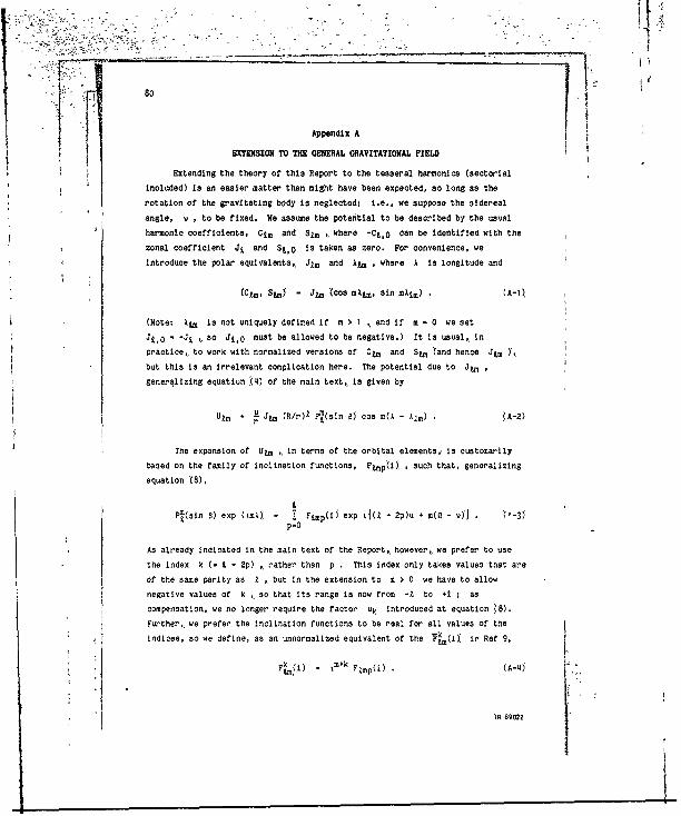
1+ 80- !Appendix A
EXTENSION TO THE GENERAL GRAVITATIONAL FIELD
Extending the theory of this Report to the tesseral harmonics (sectorial
included) is an easier matter than might have been expected, so long as the
rotation of the gravitating body is neglected; i.e., we suppose the sidereal
angle, v , to be fixed. We assume the potential to be described by the usual
harmonic coefficients, Cim and Sim , where -Ci.0 can be identified with the
zonal coefficient Ji and SZ, 0 Is taken as zero. For convenience, we
introduce the polar equivalents, Jim and Xtm , where A is longitude and
(Cim, Stm) - Jim (cos mAtm, sin mAm) . (A-i),
(Note: Xam Is not uniquely defined if m > 1 , and if m - 0 we set
Jto- -J ,, so JO must be allowed to be negative.) It is usual, in
practice,, to work with normalized versions of Cix and Sim Zand hence Jm,
but this is an irrelevant complication here. The potential due to Jim
generalLzing equation (4) of the main text,, is given by
Ulm , r (R/r)k P,(sin 0) cos m(A - Xlm) • (A-2)
The expansion of Ukm ,, in terms of the orbital elements, is customarily
based on the family of inclination functions, Ftmp(i , , such that, generalizing
equation '(8),
Pm(sin 0) exp (mX - I Ftmp(il exp ;{(t - 2p)u - m(Q - v)} . '-3)p-O
As already indicated in the main text of the Report, however, we prefer to use
the index k (- £ - 2p) , rather than p . This index only takes values that are
of the same parity as , but in the extension to m > 0 we have to allow
negative values of k ,, so that its range is now from -1 to *i ; as
compensation, we no longer require the factor uk introduced at equation (8).
Further, we prefer the inclination functions to be real for all values of the
indices, so we define, as an unnormalized equivalent of the Tm5 iM iv Ref 9,
TR 8902

The 3im expansion will involve 0 as well as the other elements, to reflect
the abandonmsent or axial symmetry, but for convenience we work with 0' def'ined
a'- S jr (A-51
Then Ulm can be decomposed into I , where
Uk - u (R/01~ Jim Fm(i), Cos {kU' m(A' - Xtmil '(A-6),
this is compatible with equation (71) of Ref 9, in which Y and X were the
negatives of the present u' and 0' . (Compatibility with two other papers canbe obtained by noting that her is 14k" times the unnormalized equivalent
of the r'tmp u~,d in Ref 13, whilst Fimp in Ref 17 is identical with Fm
introduced at (A-31, here.)
Nest ie introduce quantities Atne that directly generalize the Atn of
the mai ixt, defining
Aimi -Jem (Rip)l Fkm(i) (A-7),
We also generalize Ck and Sk , by defining.) i
CfmA -cea Cjv , ku' + m(a, - t)
Sim . 'in (iv + kul - 5(5' - Xi) J ' (A-i)Y
and henceforth we will omit the superfices.
Then '(A-6) to (A-i) give
Ukn - (p/r)" Am1
CO Ai
which is a straight generalization of equation (15) of the main tent. When
m S ,k we can also generalize the preceding equation (11) by writing
11A-
1 n(R/p)l atnA s Om* ~ Ami, (A-101
TR889022

82
where At(i), is fromo the family of 'normalized' inclination functionsIntroduced in Ref 17 to generalize the Ak(i) , and atmk generalizes cit.m
the formula for atba can be inferred from equation (11) ibid. It then follows
frc~m (A-7) and (A-10) that
tM(i - tmk S cI )n At.(i' (A-lI)
It waa assumed, in (A-10),, that m S k When 0 S k S m ,a different
generalizat'on became necessary In Ref 17, leading to
Atmk - -JI (R/P)1 oimk sm-k ,(1 + C)k Akz'(i) A-2
wnere now the formula for 41mk can be Inferred from equation 013) Ibid; also
(A-7) and (A-12) lead to
-k 5iz< am-k (I + 0)k k 5(ij. y-3
For k - m , (A-12) and (A-13) are consistent with (A-li) and '(A-li),respectively, but otherwise the dual definitions of Akm W and
tmk are
distinct. A further complication is that an extension of (A-10) and C(A-111 to
negative k is not -enerally available; (A-12) and (A-13) still operate for
k<0 .with Akl S m , but there is a marked lack of symmetry between the forms
of Ak5(i) And 0iLmk for k < 0 In relation to k > 0 . The difficulty for
negative A is not too serious, however,, as Fk '(0, can then be derived from
FkI . -m F-k0, 'A-14)
By appeal to (A-14) as required, the AtmA can always be obtained. There
are advantages In the adoption of a different 'normalization' for the Ak5(i)
however, such that they constitute a fully unified family of functions, defined
for all A and symmetric in regard to the sign of A . The constants 5tk
mu.st then also be redefined, to preserve tee Atok uncanged, and the connecting
formL ae is based on (A-i10 rather than '(A-l0). !ie inti educe a variable sign
into (A-i2), to sake the atok always positive; expressed symmetrically In
regerd to the sI9T. of A , the connecting formuila 1s thea
-tk (A~k-2) Jtm (R/p)t atmk Sm L-J~ Ak (I) (A-15)
TR 89022
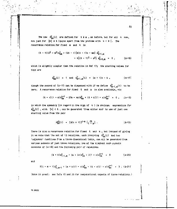
83
The new Akt(i), are defined for t Z m ,as before, but for all k now,
not just for JkI S Z (quite apart from the problem with k < 0 ,. The
recurrence relation for fixed m and k ia
(I-1)(t2
- m2)AkX. - (21 - 1)[L(l 1)0 - ok) A'.1,
11 - 1)2 - k2) Alt.2 5, - 0 , (A-16)
which Ia slightly aimpler than the relation In Ref 17; the starting values for
this are
Agm(i) - 1 and 4m+.. (i) (m +n 1) - k (A-li)'
though the second of (A-1i) can be dispensed with if we define A01 w to be
zero. A recurrence relation for fixed Zand m is also available, viz
(L. - k)(l + c)Ak+1
- 2(m - kc)Ak + (t + k)(1 - c)Ak-1
. 0 ,~ -8
in which the symmetry (in regard to the aign of k ) is obvious; expressions for,A i ,with Iki < Li can be generated 'frcm either end' by Use of just one
starting value from the pair
There is also a recurrence relation for fined t and k , but Instead of giving
it we note that t~he set of 15 relations, each involving Akn(iC and two
'adjacent' functions fom a three-dimensional table, can all be generated from
various subsets of just throe relations; one of the smpleat such subsetsconsists of (A-IA)' and the following pair of relations;
(t k)Ae..I,m t m c)Atn iCi )Atl . 0 '(A-20)
and
2(1 -m + )AkA~ (~m.+(00 - C)Akm_ - -k)C1 + )AkAI 0 . (A-20)
(Note in proof: see Refs 19 and 20 for computational aspects of these relations.)
Te 89022

We will not enlarge on the advantages of the redefinition of Ak(i) and:tmk but two disadvantages must be mentioned. First,, since the factors In a
and o in (A-15) can be combined as (1 + c)+(m*k)(I - 0)+(m-k) , we see that a
negative power of either 1 + c or 1 - c appears whenever m < ikl , and this
has to be cancelled by a corresponding positive power that is present in the new
Ak(I) . Second, the use of (A-16) and (A-17) to compute Akm(i under these
circumstances (m < ikl), is inefficient, since the recurrence process has to
work through the unwanted functions with m < t < k.
The Ak ([ are, ike the Ak(iy of the main text, defined regardless of
parity. The constants apm% (and hence the quantities Atmk ) are only definedfor Z and k of the same parity, however, and (as redefined) their only
property to be stated here is that of complete symmetry, so that
0,,1 aik ( >0). (A-22)
But, just as in the main text, we require another set of constants, alm, , and
quantities Akmr , defined when Z and k are of opposite parity, to allow the
formula for 6b to be expressed. The connecting formula corresponding to (A-15)
Is
Aim, . _)+(i-) Jim (R/plt
k sn 0, A m(1) . (A-23)
The RMu, are available at once from the auMK , since (of '26) of the main
text, which, because of the redefinition, is not being directly generalized)
oM -" Ci-1,m,"C (A-24)
Tables and further properties of the redefined inclination functions, and the
associated ronstants, will be given in a separate paper.
By making use of the quantities A mk and Aim< e we find no difficulty on
extending the theory, largely because the treatment of (p/r)t'I , in '(A-9),, via
the Btj , goes through unchanged from the main text. Further, the energy-based
exact quantity, al is still available, followirg the assumption that the
attracting body does not rotate. Thus, equstions (65), (76), (88) and (105), for
6a , de/dy , d ,/dv and M/dv , espectlvely, nrc a nchanged apart fro= the
appearance of Atmk in place of Ai0 . Equation (e2), for du/d , requirec a
T 59 ? !

85
- corresponding change, such that the derivative Aiak replaces Aim This justleaves (79), for di/dv , for which a slightly more c-aplicated expresaio' is now
required, to reflect the fact that pc2
is no longer an Invariant. We have, In
fact,
- npo A0mk I Bij Sj . (A-25)
dv
From this, using the version of dp/dv corresponding co equation (74), we get
dv s1(kc - M) Ak I Btj Sj (A-26)dv
in comparison with equation (79), we see that the only additional change is the
replacement of ko by kc - r .
Six of the seven formulae that define 8r , 6b and 6w completely, for
.,.e zonal harmonics,, are immediately applicable to the zonal harmonices, so long
as Atmk replaces Aim and the trigonometric argument includes the term
m(Q' - im) . These six are (131) and (156), for the general 6r and 6w , and
(182), (184), (192) and (194), the four special formulae for 6w . In tha
seventh fornula, (1140) for Ob , t At must be replaced by (Z - m)At,, , in
addition to the inclusion of the extra term in the trigonometric argument. (It
Is, perhaps, suprising that the change to (140) is as slight as this, but it
would have been even less if At, and Aim, had been defined to include the
factors t and I + m respectively; the reason for excluding these factors
was, essentially, to give a degree of homogeneity to (26) and (A-24.1
Finally,, of course, the numbers of terms in Or , db and 6w , for a
given Jim , are greater for m > 0 than for m 0 o , to reflect the distinctionbetween poaitive and negative a . Thes6 numbers are otherwise independent of
m , however, in consequence of which we write the formulae as follows:
Nir . 2i2 - 30 2 1 ,, IA-27)
Nib . 2t2 - 3Z * 2 (A-18) 4
and
22
for odd ZNzw - j2(Z2 - 1) for even t (A-29)
TR 89022

6 86
Appendix B
THE QUANTITIES Bjj , AND BO,1 IN PARTICULAR
When j 1 0 , Btj may be expressed in terms of the hypergeometric
function as:
SBtj A (t 1 m(,/2)J F 1 s" - i jO '2
,J ;e2).(B-)
where (B-i), applies for all Z . This result is proved, in terms of the functionSBj(e , in Appendix E of Ref 4; it ia also quoted, in terms of the equivalent
Hanson function, at equation (32) of Ref 8. For (0 S ) j < . ,, (B-1), gives a
polynomial in e2 ; for j Z i > 0 It gives zero; and for Z S 0 It gives a
power series In e2 , which can be transformed into a closed expression involving
q '(- V0 - e2)) and perhaps 8 (- e/Cl + q)) . All this is consistent with
Table 4.
Equation (B-1) breaks down when j < 0 , owing to the eventual occurrence
of a zero denominator when the hypergeometric function is expanded. Since
Btj - ,, ,, (B-2)
however, this break-down is of no account. The justification of (8-2) comes from
the Hansen-function equivalence and the relation
xii - x!-j B 3
n35 -f thBmll txtwhich follows immediately from the deflnition of Hansen's functions by equation(35) of the main tent.
The quantity Bo,j is of particular interest, being the simplest of the
Bj that involve 8 . Once it is known, the other such BZj can be
progressively derived using the recurrence relations of the main text.
From (B-1) we have
BO, - - +eF(,, 1+; 2; e2) , (B-4)
TR $9022

i 87
But as a particular case of the hypergeometic relation proved as equation (9.2)
of Ref 18, we have
F(i, 1+; 2; e2) - 2q"lF(+, 1; +; q
2) - 2F(1O, 1+; 1+; q
2) (B-5)
Also, it is immediate (from the expansion) that
F(a, b; a; q2) . (1 - q2)-b , (B-6)
independently of a , so that (B-5) gives
F(1, 1+; 2; e2) - 2/q(l * q) . 13-7)
FUpily, (B-4) and (B-7), give
B0,1 - - 1, (B-8)
in conformity with the entry in Table 4.
TR 89022
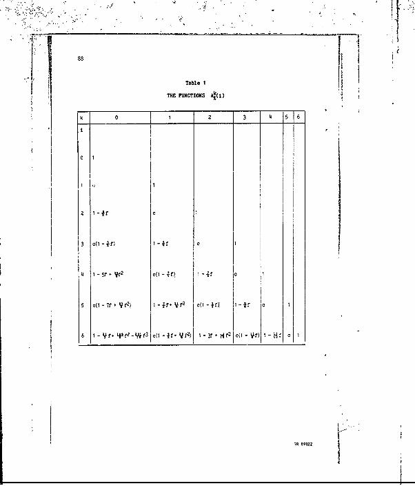
88 THE FUNCTIONS Alk(i)
kO 1 2 3 5
0 1I
2 1 -+f c1 I
5 c(l - 7f-V f2), 1-f. 4f
2 c(l - 4f)" i
6 1 9 f+Lp r-1W f3
c(1-4f V f2
) I - 3f + ?f2
c(1-V r) i-~ H 1
TA 89022

$
89
Table 2
THE CONSTANTS a& AND a..k
k/ 0 1 2 3 4 5 6
' 5 105 sos 315 231 231" T --52- "-3- 12 15-' " -2
-6 15 _ 35 a3 63
5 3 is is 3 35
4 + -2 4~~
j:-- -3 3
2
3 5
-1 1
4 3I 153
1 -- 1
2 -- --f
~ + 15 35 6
6 - - 315 2311 "NT53 T91 5
Tr 69022 i

90 Table 3 i,I I THE FUNCTIONS Bi(e) I
.1 0 1 2 3 4Z 6i
2 1 1
2 1 ,+21 +0
5 l1+3e2 +44 I + e2 I +1e
6 1 +562
. i04 I 1+ e2
+ j04 .+ e2 1 + je2
I1
7 1 ye2 +44e4 +AO6 1 + +e2 + e4 a~2
+A e4 + .e2
1 + e2
1 1
TR 89022

-Table
TH QUANTITIE 8
0 2
1 0 1 2
2 0e 1 0e 0 0
3 e 4(2 -e2), e 4e
2 0
4 4e(O A J< 42 - 3A) 4e(4+ e2) 4e2
e
TR 89022

92
Table 5
THE QUANTITIES EM
k 0 1 2 3
-3 3eq-5
-fq-5
(4i 3e2) 5eq-
5 -e 2q-5
-2 eq-3
-4q-3
e-
*-1 0 -q-1
0 0
I e
2 3e (I . 2e2)
3 +.e(4 . e2) 1 4 ~2 I-e(2 , 3A2
'4 .e('4 * 3e2) 7-4*~e2
* 4e4) L.e(2 + 5e2), je2(3 + '4e2 )
TR 89022

93
Table 6
THE NUMBER OF TERMS IN 6r, 6b AND 6w
• N,r 1 ,b Nz,w
1 0 1 1
2 2 2 3
3 5 6 9
11 11 15
5 18 19 25
6 28 28 35
7 39 40 49
8 53 53 63
9 68 69 81
10 86 86 99
11 105 106 121
12 127 127 143
13 150 151 169
14 176 176 195
15 203 204 225
16 233 233 255
TR 89022

94i
LIST OF SYMBOLS
(Usage for the main text only)
a SeMI-Major axis
energy-based fixed value of a
At(i) 'normalized' function of inclination
A&k quantity,, based on Ak(i) , defined by (14)
At, similar to Alk , but defined by (17)
Aik derivative of A with respect to I
A& k3-1 AUk t a-) A <
b latitude-like spherical coordinate of (r, b, w)
8j(e) normalized function of eccentricity
Btj quantity related to 8 (e) , defined by 32)
6 derivative of Bij with respect to e
o cos i
C(or Cj) cos (jv - kul) ,(dtfferent meaning in Part 1)
d shorthand for k - j - 1 etc in sections 7.4 and 7.5
Ot(i) inclination fanction, quoted from Ref 4
e eccentricity
E eccentric anomaly (only required in section 8)
TR 9022"

95
LIST OF SYBL cniud
Ej(e) eccetriity function, quoted from Ref 4 *Ejj qiantityrelated to Eejdefined by (48)
G ~ n*-J4 (R/p)4
(in section 8.5)
h angular momentum (but I - +f in section 8.3)
H +. J3 (R/p)3,(in section 8.4)
I Inclination
index asscciated with multiple$ ofv
JZ zonal harmonic coefficient for the Earth
k Index associated with multiples of u
K + J2 "(R'p)2
'(in section 8.3)
9. Inden of JZ
L quantity su~h that L- *q - n*
m v - M in section 8.5 (and Part 1); otherwise ant arbitraryInteger
M mean anomaly
n mean motion
TR sc022

r{
!! 14
We will require derivatives of the inclinatlion functions. It is evident
from (10) that
d [kj) UI - k)(t , k + 1) 5 kh1 (18di i 2(k * 1) a
from this and ,(14) it follows that the (partial) de~ivative of Ak with respect
to i is given by
(/p {ko A (i - (Z - k)1 k + 1) fA '(19)
where f - S2 The quantity in (curly) brackets is the Db(iY of Ref A. We
will also require, finally, the particular combinations of Ate and AU
denoted by A;k and Atk , and given by
Ak - ks-1
ANk a 0-
Aik , (20)
the s-1 and c
-1 factors do not mply singularities, as they must always
cancel via < AUk and Ajk respectively.
The Ak(iY and a~k (and hence the Att 'm nay be computed with the aid of
recurrence relations. A fixed k was stipulated in Ref 4 for the formula
(i + k) A (i) - (21 - 1) c Ak.1(i) - - < - k) A(2 (i) , '21)
valid for A k + 2 with the starting values Ak(i) - 1 and A. 1(i) -
(21) is even valid for A - K + 1 , if an awbitrary (but finite) Ak_1(i) is
assumed. However, it is usually more useful to stipulate a fixed A , the
*aqucred formula wag giver by Merson11
, being
Ak(-) k cA ,) (Z - < - )I + ) f 2) f +2(i)(22)
valid for Z - 2 1 k A 0 with the starters A ( - 1 and A[-1(i) -
(221 is alo valid for k - A - 1 ,, with an arbitrary (finite) A ,i) . Either
of the two preceding 'pure' three-term recurrence relations, (2,) or (22), can be
,soa with just one 'miAed' such 'elation to genorate all the relations cornecting
the A(i) . perhaps toe simplest -ixei relation (with neitner Z nor k fixed)
89
TO 39022

tit~
96
LIST OF SYM4BOLS (continued)
Nt,r- Nt,b- Nt,w numnber of terms (for given L) in 6r, 6w. it
p ~ parameter (aemi-latus rectum) of orbit
V Legendre polynomial (of argument aupplied)
q vo - e2),
Qj(e) normalized eccentricity function Quoted from Ref 3
r radius-vector coordinate of (r, b, W1
j i Earthas equatorial radium
Ri(for Rk quantity defined by (125Y '(different in Part 1),
3 sin I
S (or Sj) ain Qv , kW) '(different meaning in Part 1)
t time
rj (ror Tjj quantity defined by (137)
u argument of latitude, v -
Umodifier' u (- V wu' -u
UZ ~ potential due to J
Z component of Ut
R 89022 ~ '~

97
LIST OF SYMBOLS (continued) [Vtrue anomaly
v orbital speed (used only in section 8)
Vjpj Vj,a. Vj,-.. quantities introduced at (1149),
w longitude-like spherical coordinate of (r, b, w)
WIO. Wt...i quantities Introduced at (153)
x, y general unknown quantities (different in Part 1)
Xmi generic Hansen function (of eccentricity),
Z -J, R (section 8.2)
Rk fixed constant, defined by (12)
so~ fined constant, defined by (16)
a geocentric latitude (declinatifin); e/0l q) in sectlon 3
1 symbol fo- pur'e short-pe. Lod perturbation (6p in Part 1),
C generic orbital element (osculating)
mean element correspcncing to
seni-nean elemnt
rate ofchange of -t due 'o Ut
TR 69022

98
LIST OF SYMBOLS (concluded)
'K Index related to k, but of opposite parity
A -J, R/p (section 8.2)
u Earth's gravitational constant
P quantity such that + q*
modified mean anomaly at epoch
summation (different use of I in Part 1)
Uk I If k - 0, 2 if k > 0
quantity such that + ch o
argument of perigee
TR 89022

Y--
99
REFERENCES
No. Author Title, etc t1 R.H. Gooding Satellite motion in an axi-symuetria gravitational
field Part 1 Perturbations due to J2 (second
order) and J3
RAE Technical Report 88068 (1988)
2 R.H. Gooding Complete second-order satellite perturbations due toJ2 and J3 , compactly expressed in spherical-polar
coordinates.
Acta Astronautica, 10, 309-317 (1983)
RAE Technical Report 83033 (1983)
3 R.11. Gooding On mean elements for satellite orbits perturbed bythe zonal harmonics of the geopolential.
Adv. Space Roe., 10, 279-283 (1990)
RAE Technical Memo. Space 371 (1989)
4 R.H. Gooding Satellite motion in an axi-symmetric field, with an
application to luni-solar perturbations.
RAE Technical Report 66018 (1966)
5 R.H. Gooding On the generation of satellite position (andvelocity) by a mixed analytical-numerical procedure.
Adv. Space Res., , 83-93 (1981)RAE Technical Memo. Space 311 (1982
6 G.V. Groves Motion of a satellite in the earth's gravitational
field.
Proc. Roy. Soo.. A 254, 48-65 (1960)
7 W.M. Kaula Theory of satellite geodesy
Waltham, Mass. etc., Blaisdell Publ. Co. (1966)
8 B. Zafiropoulos The motion of a satellite in an axi-symmetric
gravitational field.
Astrophys. Space Sol., 139, 111-128 1987)
9 R.H. Gooding A second-order satellite theory, with compact results
in cylindrical coordinates.
Phil. Trans. Roy. Soo, A 299, 425-74 '(1981)
R 90
pe 8oon

100
REFERENCES (continued)
NO. Author Title, etc
10 R.H. Gooding Satellite location by OPS (Navatar)
11 R.H. Meraon The dynamic model of ?80?, a computer program for the
rei2mn of.P e th ria armtr fa earth
satOrbital
RAE Technical Report 6650431987)
ewhoreeDoverc PublimdmClatial 60 fo Ch. (1918)
D.G. Kin-The motlyion of a 010m esathlltelorite.
Proc. Ro. S0., A, 214 1-25 (198)
RAE Technical Reot 8805 (198),
17 R.H. Gooding Anirersarenceureio for cinarion ofuorbta
eleaeta teho an , 9f-om poi1971)vloit
RAE Technical Report 70743 (197)
18 Y.. Snddn Soal Th notiono of m ls athmatcal ie.ln
omAstr.J.6436-709)
17 RH. Godin ASecnd n edi ation fprntd) Edcinbtigh antions.
-Oliver and Boyd (1966) m02

REFERDICES (concluded)I
NO uhrTitle, ae j19 J.B. Lundberg Recursion formulas of Legendre functions for use with
B.E. Schutz nonsingular geopotential models.
j. Guidance, 11, 31-38 (1988)
20 W. Gautschi Cesputational aspects off three-term recurreacerelations.
SIN eview, 9,24-82 (l967)
- ~ ~ I "39022

'a hi 0.. toventer eantyceninformationhthe bo
It s~tirsibte t'.e page should cotn ol nauidnotto.hta eese oetrdnildifnatn h o
roovjon h eake t~'dkat taecaafcloee.RtreConfidential orSecret.
L'i.DltlCReferone . [. reateaReeec, Agey 4.RprtScrty Clatta ficttrlna~ ~ deabl~l)~ I ~ ~ ~ I? {Ree~eee
767000 11ants UK
Sa Sontolng genc a Cde d. Spetorng Aea~.~Conrac Auh rit)ne and Location
7 Tritle, Satellite mtion int ain axi-asyneti, iiviiational, field
4b.'(For Copference Pspers) file. Plac and Date of Cnfire
&Aithr~.5Iuanindllas 0a..Auth~r2 9b.' Autho-tn3,4-... 10. Date . -R
.Gcbdat~,;1l98 101
1'CntptNrnhr I2.Perlodl 1 3.,Project 14. Other Reference Not.Space 675
IS lsirbitiaarnieo
(bi) Special U:4ationa (Ir any) -If at 1s inlerded hirst a c* of this dlocumnta shall le released ov~rat refer to RAE Leaflet No.3 to Supplement 6 of
16.tl~ru~oto(l~)~yr is) . Dectiiite amhed5
r selected from TISM)Asc yrnja celestial inichanics GeopotntiAl GiraViatientil effects) ,
Saie,.l't Or;ts fbit; calculations5 Orbit perturbation. Satelip e orbit:%0
.Il ea)otur;Lations. Zonal harmonics. 4W4f 7~~*' d .
'>Tr z Report cotinues con lh.,preisentation of the untruncated orbital theorybegun it ecchnie.-l Report 8068. The effects of the general tonal bansconic, JL
arcow .,overed, the wain results; being a trio of formnulae ftr pett bations in the
speialp l irdinates introduced in the previousppr. heoruaaeonly first-order in Tp , buat, in conjunction with the second-order resalis for J2published in Part -1 then corriate set of formulae ;Aay be regard2d as constituting a
I aeicond- ) -dor theory,"tbe E~rtliS s J' being Patch larger ilton _Jt f,.r t > 2
The mean elements of the theucry are aefinod in such a way thet., for eachthe coordinate-petturbat.on for=,xlae have their siretlanst possl~e form, with
no occurrence of zero denot~inatrors. vle general formuilaes are used Ln a raeoriva-tion of tie resuitis for 7, , qiven in Part 1, and in as dorivation )f results fnc
Z24 Numerical comparisons with reference orbits are hold ove:- to a later report
RlAE lPoin At43 (evtaediiciobei tit)