aviation infrastructure performance and airline cost: a

Aviation infrastructure performance and airline cost: astatistical cost estimation approach

Mark M. Hansen *, David Gillen, Reza Djafarian-Tehrani

Institute of Transportation Studies, National Center of Excellence in Aviation Operations Research,

University of California at Berkeley, Berkeley, USA

Abstract

The relationship between the performance of the US National Airspace System (NAS) and airline costs isexamined by estimating airline cost functions that include NAS performance metrics as arguments, usingquarterly data for 10 US domestic airlines. Performance metrics that vary by airline and quarter are de-veloped by applying principal component analysis to seven underlying variables, including average delay,delay variance, and the proportion of ¯ights that is cancelled. This analysis reveals that variation in theseven variables can be adequately captured by three or fewer factors, which we term NAS performancefactors. If three factors are used, they can be interpretted as ``delay'', ``variability'', and ``disruption'', thelatter two of which are merged into a single ``irregularity'' factor in the two-factor model. Cost functionestimation results con®rm the anticipated link between NAS performance and airline cost. In the costmodels with two and three performance factors, the irregularity and disruption factors are found to havethe strongest cost impacts. These results challenge the prevailing assumption that delay reduction is themost important bene®t from NAS enhancements. Using the estimated cost models, we predict airline costsavings from substantially improved NAS performance in the range $1±4 billion annually. Ó 2000 ElsevierScience Ltd. All rights reserved.

1. Introduction

The need to understand and quantify the bene®ts of public and private investments in theNational Airspace System (NAS) has never been greater. On the public side, executive order12893, published in 1994, requires the Federal Aviation Administration (FAA) along withother federal agencies to conduct systematic analysis of bene®ts and costs of all infrastructure

Transportation Research Part E 37 (2001) 1±23www.elsevier.com/locate/tre

* Corresponding author. 107B McLaughlin Hall, Berkeley, CA 94720, USA. Tel.: +1-510-642-2880; fax: +1-510-642-

1246.

E-mail address: [email protected] (M.M. Hansen).

1366-5545/00/$ - see front matter Ó 2000 Elsevier Science Ltd. All rights reserved.

PII: S1366-5545(00)00008-9

investments involving annual expenditures in excess of $50 million. The analysis is to ``quantifyand monetize bene®ts and costs to the maximum extent possible (FAA, 1998)''. Moreover, theFAA acquisition management system, published in 1997, mandates an ``investment analysis''prior to the initiation of a new acquisition program, including, among other things, the identi-®cation of alternatives and assessments of their bene®ts and costs (FAA, 1998). Such analyses arerequired for a host of Air Tra�c Management (ATM) and Communications-Navigation-Surveillance (CNS) programs through which FAA intends to modernize the NAS over the nexttwo decades (FAA, 1999).

Private investments, particularly those by airlines in advanced avionics for new aircraft, are alsogetting closer economic scrutiny. According to Allen et al. (1998), ``the industry is getting to thepoint where the achievement of business case maturity may be more important than technicalmaturity''. Business case maturity includes the ability to explicitly identify bene®t mechanismstriggered by CNS/ATM investments, credible estimates of the dollar values ¯owing from thesemechanisms, and explicit analysis of investment risk (Allen et al., 1998). The CNS/ATM focusedteam (C/AFT), whose membership includes airframe manufacturers, airlines, and the FAA, hasbeen working since 1997 to develop and apply a methodology for developing such business cases.

While the need for bene®t quanti®cation is growing, industry stakeholders are also recognizingthat the performance of the NAS is multi-dimensional, and therefore not adequately captured bytraditional, delay-based, metrics. For example, the C/AFT has identi®ed six categories of per-formance, including, in addition to delay, predictability, ¯exibility, e�ciency, access, and cost ofservice (Alcabin, 1999). These concepts are considered to ``de®ne the elements of value to thescheduled airline business'' as well as ``the common criteria for developing economic modelsneeded to predict bene®ts. . .(Alcabin, 1999)''.

Taken together, these trends imply a need for bene®t valuation methodologies that incorporatemultiple dimensions of NAS performance. The purpose of this paper is to demonstrate one suchmethodology, based on statistical cost estimation. The work presented here builds on an earlieranalysis by Hansen, Gillen, and Djafarian-Tehrani (forthcoming) that employs simple Cobb±Douglas (log-linear) models. Here, we employ translog models and more sophisticated estimationtechniques. However, our key results are largely consistent with those in the earlier work.

In Section 2, we review and critique existing bene®t valuation methodologies, and suggestvarious ways of improving them. In Section 3, we overview the approach adopted in this paper,the essence of which is to incorporate NAS performance metrics into airline-level cost functions.Section 4 presents our methodology for developing the performance metrics, while Section 5discusses the speci®cation and estimation of the cost function. Estimation results are considered inSection 6. In Section 7, the results are used to estimate industry cost savings from improved NASperformance. Section 8 concludes the paper.

2. Review and critique of current practice

Despite wide acceptance that NAS performance should be characterized in a multi-dimensionalway, such a view is largely ignored in present-day investment analysis. Almost without exception,investment analyses and business cases consider only delay and direct cost savings when evalu-ating the bene®t of an NAS improvement. For example, a recent business case for advanced data

2 M.M. Hansen et al. / Transportation Research Part E 37 (2001) 1±23

link (ATS Data Link Focus Group, 1999), considered to be a path-breaking e�ort within theindustry, identi®es four bene®t categories. Two involve communication cost savings, one is in-creased availability of communication between aircraft and airline operation centers (this wasguessed to be worth anywhere between $16 and $48 per ¯ight), and the last category is delay costsavings (valued at $25 per min based on aircraft direct operating cost).

Thus, even as industry stakeholders recognize that NAS performance has many aspects, onlydelay is routinely monetized. Even here, however, there is ample room for skepticism about theprocedures. Virtually all delay cost calculations involve nothing more than the application of acost factor based on reported values for the average direct aircraft operating cost per block hourto quantities of delay measured in time units. For air transport aircraft, the cost factor is in therange $20±25 per min. A few studies re®ne this ®gure by di�erentiating between delay taken at thegate, on the ground, and in the air (Geissinger, 1988; Odoni, 1995). Others extend the calculationsby disaggregating expense by functional category, such as fuel, ¯ight personnel, maintenance, andcapital, and estimating how delay, portrayed as changes in the quantity of block hours, a�ectseach one (Kostiuk et al., 1998).

These approaches to delay cost estimation are based on strong assumptions that are rarelyscrutinized or even acknowledged. These include that the cost of delay is an additive function ofthe cost of individual delay events, and that the cost of each event is a linear function of theduration of the delay (perhaps taking into account the phase of ¯ight in which it occurs). Suchassumptions ignore the possibility that delay cost is non-linearly related to duration, subject tocombinatorial e�ects, and includes sizable indirect components.

It is probable that the cost of a delay varies non-linearly with the duration of the delay. Forexample, one 40-min delay is likely to be more costly than 40 one-min delays. The 40-min delay isfar more likely to disrupt ground operations, gate assignments, crew schedules, and passengeritineraries. Conversely, airlines sometimes add delays to ¯ights in order, for example, to avoidhaving a ¯ight arrive at a hub in the middle of a departure bank. If this is rational behavior, thenthe relationship between cost and delay must not only be non-linear, but also non-monotonic.

Delay costs are also subject to combinatorial e�ects. The severity of the impacts noted above islikely to depend not only on the duration of delay to a speci®c ¯ight but also on the interaction ofdelays for many ¯ights. This is particularly evident in a hub-and-spoke network in which ¯ightsare scheduled in connecting banks. If all the ¯ights in an inbound bank are delayed by the sameamount, then the e�ect may be far less severe than if half the ¯ights are delayed by a larger (oreven the same) amount.

Finally, the prevalence of delays may generate sizable indirect costs through airline adaptationbehaviors. Carriers may take a variety of measures to make their operations more robust to delay.These include building more padding into scheduled block times, providing ¯ights with additionalfuel, and having extra aircraft, ¯ight crew, and ground personnel available. While these measuresdecrease the cost of delays when they occur, they also increase costs of day-to-day operation. Inthis way the cost of delay may permeate throughout the entire cost structure of the airline in waysthat are not tied to individual delay events.

Our limited ability to take these aspects of delay cost into account, combined with the nearlycomplete absence of information on how to place an economic value on other dimensions of NASperformance, represents critical gaps in knowledge at a time when massive investments in thesystem are being contemplated. One might attempt to ®ll these gaps in a variety of ways.

M.M. Hansen et al. / Transportation Research Part E 37 (2001) 1±23 3

Simulation is one possibility. To address the questions under consideration here, a simulationwould have to be highly detailed. It would need to capture how airlines respond on a real-timebasis to operational irregularities and the cost implications of that response. The problem getsespecially complicated when major adjustments such as rerouting of aircraft and reassigning crewsare considered. While such a simulation may eventually be possible, it is beyond our presentcapabilities.

A second possibility is to systematically query airline personnel. For example, one mightpresent dispatchers with di�erent scenarios concerning the operation of their assigned ¯ightsthroughout the day or month, and ask them to choose which scenarios are more desirable. If thescenarios were carefully chosen, this procedure would reveal the preferences of the participants,and thereby allow the estimation of utility functions whose arguments would be various dimen-sions of NAS performance. Such a study might yield useful results, but is also subject to a numberof objections. First, it is not clear how such a methodology could allow monetary valuation ofNAS performance, since this would require participants to choose between scenarios that involvemoney as well as ¯ight operations. Second, it is not obvious that dispatchers, or any other airlinepersonnel, have su�cient knowledge of the airlineÕs interest to make choices that accurately re¯ectit. Finally, the results of such a study might be biased by principal/agent e�ects, with respondentsmaking choices that are best for them rather than for the airline as a whole.

This paper focuses on a third approach, which is to estimate airline cost functions includingNAS performance measures as arguments. Using published, quarterly, airline-level data, we es-timate relationships between airline operating expense, outputs, factor prices, and other variables.Included among the latter are a set of variables, which we term ``NAS performance factors'', thatquantify the airlineÕs operational experience in the NAS during the quarter. By observing howthese variables in¯uence airline expense, we establish a direct empirical basis for translatingvarious dimensions of NAS performance into monetary terms. Any quanti®able aspect of NASperformance can, in principle, be accommodated in this framework. Moreover, because rela-tionships are derived from observed co-variation between performance variables and cost, theresults entail a minimum of assumptions about the mechanisms involved.

This paper presents the ®rst step in using cost estimation to assess the economic value of NASperformance. It employs a relatively small data set and, accordingly, a limited set of NAS per-formance variables and a simpli®ed form for the cost function. Nonetheless, it yields plausibleresults, including industry-wide estimates of the costs from ``sub-optimal'' NAS performance thatare comparable with results of more conventional studies based on delay cost factors. This sug-gests that statistical cost estimation is a promising avenue for assessing the economic bene®ts ofNAS improvements.

3. Cost estimation approach

The cost function of a ®rm is de®ned as the lowest cost at which it can produce a given set ofoutputs, ~Y , given the prices it pays for inputs, ~P . Equivalently, it represents the cost of acquiringthe optimal set of inputs, ~X �, given the outputs and prices. Thus we have

COSTit � ~Pit � ~X ��~Yit;~Pit� � C�~Yit;~Pit�; �1�


where the subscript i denotes a particular ®rm (airline), and t identi®es the time period. The costfunction, like the production function, is a way of depicting the technology available to the ®rm,i.e., its ability to transform inputs into outputs. Implicit in (1) is that all airlines have the sametechnology, an assumption that could be relaxed by adding airline subscripts to the cost andconditional demand (~X �) functions.

Eq. (1) can be considered a long-run cost function because it assumes that all inputs have beenadjusted to their optimal levels. Some inputs, particularly capital inputs, cannot be varied in-stantaneously. A short-run cost function relaxes the assumption of optimal capital stock bytreating capital as a quasi-®xed factor and removing capital costs from the dependent variable.This results in capital being an argument in the short-run, or operating, cost function. Thus wehave

OCOSTit � ~Pit � ~X ��~Yit;~Pit;Kit� � O�~Yit;~Pit;Kit�; �2�where capital is excluded from the price and conditional demand vectors.

It has long been recognized that costs depend on the nature and quality of airline outputs aswell as the quantity. For example, airlines have been shown to have economies of density,whereby the cost for a given total output increases with the size of the airlineÕs network. Severaladditional variables are included to capture such e�ects. These are incorporated into the vector~Zit.This yields a short-run cost function of the form O�~Yit;~Pit;~Zit;Kit�. This form, as well as the long-run version in which capital is not an argument, has been widely studied in the airline economicsliterature (Caves et al., 1984; Gillen et al., 1990; Hansen and Kanafani, 1990; Encaoua, 1991;Windle, 1991), and serves as the point of departure for the present study.

In this study, we add one additional vector argument, ~Nit, which characterizes airline iÕs op-erational experience in the NAS during time period t. In general, ~Nit is based on variables such asaverage delay, delay variance, and the proportion of cancelled ¯ights. It can be viewed as theperformance of the NAS from the standpoint of an individual airline. This is not to suggest that~Nit depends only on the performance of public aviation infrastructure; rather it derives from theinteraction between that infrastructure and operational decisions taken by the airline. ~Nit may alsobe a�ected by factors completely unrelated to the infrastructure, such as mechanical problem,labor actions, or severe weather. Nonetheless, both public and private investments in the NAS areprimarily intended to change ~Nit for the better.

Thus, our analysis revolves around estimating the operating cost function O�~Yit;~Pit; ~Qit;Kit; ~Nit�.The ®rst four arguments are standard ones in the airline cost estimation literature. The last, whichis the focus of our investigation, implies a relationship between NAS performance, measured atthe airline-level, and airline operating cost. In order to quantify that relationship, one must ®ndand develop an ~Nit vector which captures airline-level NAS performance in a compact, yetcomprehensive way.

4. NAS performance measurement

Our measures of NAS performance are derived from the operational experience of airlinesusing the NAS, as captured by such metrics as average delay, variability of delay, and ¯ightcancellation rates. As noted previously, these measures not only re¯ect the quality of service


provided by the public aviation infrastructure, but also the airlinesÕ ability to plan and managetheir operations. Both of these factors depend on exogenous events, particularly weather, as wellas the competence (and perhaps luck) of service providers and users. Thus, when we refer to highor low performance levels, we are not a�xing credit or blame to either the FAA or the airlines,but rather assessing operational outcomes in which both, along with a host of exogenous factors,play a role.

We must quantify NAS performance by airline and quarter, the smallest time unit for which®nancial and tra�c data are available. To do so, results for thousands of ¯ights must be sum-marized by a much smaller set of metrics. There is no uniquely valid way of doing this. One might,for example, base metrics on the ¯ight, the ¯ight complex, the day, or the airport-day. (Toillustrate the last possibility, one might categorize for a particular airline, airport, and day as``smooth'', ``mildly irregular'', or ``highly irregular'', determine the proportions of airport-days ineach category, and use these as the performance metrics.) Here, we opted for the more conven-tional ¯ight-based approach, reserving the others for subsequent work.

Even while con®ning ourselves to ¯ight-based metrics, there is a huge number that might beemployed. To keep the analysis tractable, we employed a two-step approach. In the ®rst step, weevaluated seven metrics for each airline and quarter in our data set. Next, we employed principalcomponent analysis to collapse these metrics into a smaller number of factors, and calculated thefactor scores for each airline and quarter. These factor scores were used to compose the ~Nit vectorused in the subsequent cost estimation.

The seven underlying metrics are de®ned in Table 1. The ®rst two metrics pertain to delay, andare thus the most closely related to the conventional approach for measuring NAS performance.The third metric focuses on more extended delays, which, as argued above, may have qualitativelyand quantitatively di�erent impacts on costs. The next two metrics re¯ect variability in ¯ightoperations. The sixth metric is the standard metric for service reliability; it depends on both themean and the variance of delay. The ®nal metric re¯ects the incidence of conditions whenoperations become su�ciently irregular to result in ¯ight cancellations. All of the metrics wereevaluated by airline and quarter ± for the 11 quarters extending from the winter of 1995 throughthe summer of 1997 ± using the airline service quality program (ASQP) data base, which presentsscheduled and actual departure times for every domestic ¯ight of the top 10 US carriers. Thus, ourdata set includes 110 observations. Since we employ a log-linear cost function speci®cation, andall metrics were consistently positive, logarithms of these metrics are used in the subsequentanalysis.

Table 1

Performance metric de®nitions

Variable (in log form) De®nition

Average arrival delay Di�erence between scheduled and actual arrival time, averaged over all ¯ights.

Average departure delay Di�erence between scheduled and actual departure time, averaged over all ¯ights.

Average >15 min arrival delay Sum of all arrival delays in excess of 15 min, divided by total number of ¯ights.

Arrival delay variance Variance of the di�erence between scheduled and actual arrival time.

Departure delay variance Variance of the di�erence between scheduled and actual departure time.

Unreliability Proportion of ¯ights with an arrival delay over 15 min.

Cancellation rate Proportion of ¯ights cancelled.


As shown in Table 2, the seven performance metrics are highly inter-correlated. All correlationsare greater than 0.4, and the majority in excess of 0.6. This suggests the use of principal com-ponent analysis as a way of capturing most of the information contained in the seven performancemetrics in a smaller number of variables. Principal component analysis identi®es a set of factors ±linear combinations of the original variables ± which together account for as much of the totalvariation in the original data as possible. The factors are obtained by ®nding eigenvectors of thecorrelation matrix. The higher the eigenvalue, the greater the explanatory power of the associatedeigenvector. By convention, each factor has zero mean and unit variance. By virtue of beingeigenvectors, the factors are also mutually orthogonal.

The results of the principal component analysis of the NAS performance data are summarizedin Table 3. The ®rst component has high, positive, loadings on all seven factors and accounts for72 percent of the total variation. The second factor, which accounts for about half of the residualvariation, has positive loadings on the variance metrics and negative loadings on delay and un-reliability. Thus, airlines scoring high on this factor tend to have unusually high delay variancesand/or unusually low delay averages. The third factor explains eight percent of the total variation,and has a high positive loading on ¯ight cancellations and a negative loading on departure delayvariance. Altogether, these factors explain about 94 percent of the variation in the total data set.

In principal component analysis, the standard procedure is to determine the number of factorsto be extracted from the data, and then rotate these factors so that factor loadings are close toeither 0 or �1, in order to simplify their interpretation. In choosing the number of factors, one

Table 2

Performance metric correlations

Variable (in log form) ADD AAD A15AD ADV DDV UNRE CANR

Average depature delay (ADD) 1 0.82 0.83 0.54 0.53 0.53 0.81

Average arrival delay (AAD) 0.82 1 0.83 0.47 0.51 0.43 0.93

Average >15 min arrival delay (A15AD) 0.83 0.83 1 0.85 0.75 0.66 0.90

Arrival delay variance (ADV) 0.54 0.47 0.85 1 0.80 0.65 0.57

Departure delay variance (DDV) 0.53 0.51 0.75 0.80 1 0.44 0.60

Unreliability (UNRE) 0.81 0.93 0.66 0.65 0.44 1 0.53

Cancellation rate (CANR) 0.53 0.43 0.90 0.57 0.60 0.53 1

Table 3

Results of principal component analysis

Variable (in log form) Factor 1 Factor 2 Factor 3

Average arrival delay 0.85468 )0.46316 )0.05345

Average departure delay 0.86167 )0.31608 0.07645

Average >15 min arrival delay 0.98444 0.02062 )0.03112

Arrival delay variance 0.81784 0.51105 )0.08456

Departure delay variance 0.77662 0.38233 )0.42532

Unreliability 0.91327 )0.31949 )0.02627

Cancellation rate 0.70281 0.31987 0.61739

Proportion of variance explained 0.7203 0.1324 0.0828

Cumulative proportion 0.7203 0.8527 0.9355


must make a judgment about when the additional variation explained by a factor is su�cient tojustify retaining it. In the present case, we decided to con®ne our attention to no more than threefactors, since none of the remaining ones accounted for more than 3 percent of the total variation.The choice between one, two, and three factors was more di�cult. An oft-cited rule-of-thumb is toinclude only those factors which account for more than one Nth of the variation, where N is thenumber of variables in the data set. Applying this to the present case, we ®nd that only one factorshould be retained. On the other hand, this leaves out nearly 30 percent of the variation in theoriginal data set, suggesting the possibility of adding a second or third factor. Rather than ®xingon a single alternative, we chose to estimate cost models including one, two, and three NASperformance factors.

Varimax factor rotation was then performed on the two-factor and three-factor representa-tions. The results appear in Table 4. In the two-factor case, the ®rst factor correlates more highlywith the delay variables, including the average delays, average delays over 15 min, and unreli-ability. The second factor has the highest loadings on the departure and arrival delay variances,the cancellation rate, and, like the ®rst factor, average delays over 15 min. One might summarizethis by terming the ®rst factor ``delay'', and the second factor ``irregularity''. When three factorsare used, the ®rst one is virtually identical to that in the two-factor case. The second factor is alsoquite similar, except that the loading on cancellation rate is considerably lower. The third factorhas a very high loading on cancellation rate, along with some correlation with arrival delayvariance and average delay over 15 min. The three factors might be described as ``delay'',``variability'', and ``disruption''. A carrier with a high score on the ®rst factor has ¯ights thatdepart and arrive later (relative to schedule) than those of the average carrier. If the second factorscore is high, then delays ¯uctuate more widely than average, while a high score on the third factormeans that conditions requiring ¯ight cancellation are more prevalent than average.

Figs. 1 and 2 present average factor scores for the one-factor analysis, by airline and quarter,respectively. Fig. 1 reveals that, using the one-factor analysis, the two carriers experiencing thebest NAS performance (i.e., with the lowest factor score) are USAir and Southwest, while Delta,United, and TWA experience the worst performance. Fig. 2 shows that the quarters with theworst NAS performance include the winters of 1996 and 1997, along with the summer and fall of

Table 4

Rotated factor patterns for one, two, and three factors

Variable (in log form) One factor Two factors Three factors

Factor 1 Factor 1

``Delay''

Factor 2

``Irregularity''

Factor 1

``Delay''

Factor 2

``Variability''

Factor 3

``Disruption''

Average arrival delay 0.85468 0.84848 0.34994 0.84157 0.24310 0.28441

Average departure delay 0.86167 0.94280 0.23688 0.94150 0.21837 0.11721

Average >15 min arrival delay 0.98444 0.71120 0.68099 0.70453 0.58051 0.37035

Arrival delay variance 0.81784 0.25679 0.92957 0.24960 0.82240 0.44559

Departure delay variance 0.77662 0.31348 0.80687 0.31927 0.90509 0.09532

Unreliability 0.91327 0.88880 0.38233 0.88504 0.32591 0.21751

Cancellation rate 0.70281 0.30136 0.71094 0.27235 0.25557 0.91539

Proportion of variance explained 0.72030 0.45140 0.40140 0.44470 0.30150 0.18920

Cumulative proportion 0.72030 0.45140 0.85270 0.44470 0.74620 0.93550


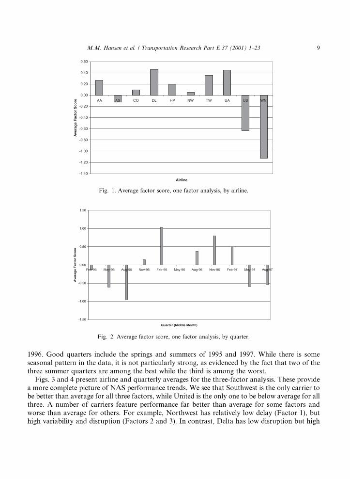
1996. Good quarters include the springs and summers of 1995 and 1997. While there is someseasonal pattern in the data, it is not particularly strong, as evidenced by the fact that two of thethree summer quarters are among the best while the third is among the worst.

Figs. 3 and 4 present airline and quarterly averages for the three-factor analysis. These providea more complete picture of NAS performance trends. We see that Southwest is the only carrier tobe better than average for all three factors, while United is the only one to be below average for allthree. A number of carriers feature performance far better than average for some factors andworse than average for others. For example, Northwest has relatively low delay (Factor 1), buthigh variability and disruption (Factors 2 and 3). In contrast, Delta has low disruption but high

Fig. 1. Average factor score, one factor analysis, by airline.

Fig. 2. Average factor score, one factor analysis, by quarter.


variability and delay. Because the factors are, by construction, orthogonal the lack of a consistentpattern in the airline factor scores is to be expected.

These di�erences among airlines may derive from either the conditions in which they operate orhow they respond to such conditions. For example, Northwest may have more variability anddisruption than Delta because it operates out of hubs in the northern US where severe stormsoccur. Alternatively, it may be that, as a matter of operational strategy, Delta is willing to acceptgreater delays in order to avoid cancelling ¯ights. These di�erent possibilities highlight the point

Fig. 3. Average factor score, three factor analysis, by airline.

Fig. 4. Average factor score, three factor analysis, by quarter.


that the factors capture the interaction between aviation infrastructure and its users, not just theperformance on one or the other.

From Fig. 4, we see that just two quarters ± the spring and summer of 1995 ± have better thanaverage performance on all three dimensions, while two others ± fall, 1996 and winter, 1997 ± areconsistently worse than average. We also see from Fig. 4 that the horri®c winter of 1996 wasparticularly bad from the standpoint of delay and disruption, but average from the standpoint ofvariability. A similar, but less pronounced pattern is seen in the winter of 1997, while in the winter1995 only disruption was worse than average. Disruption is consistently less of a problem in thespring and summer quarters, as is delay except for 1996. Finally, there is some evidence of asecular trend to worse performance on the variability dimension: four of the ®rst ®ve months arebetter than average in this respect, while each of the last six months is worse than average.

5. Cost model speci®cation and estimation

We now consider the relationship between the airline-level NAS performance factors derived inSection 3 and airline operating cost, using the cost function framework explained in Section 2. Todo this, we use the performance factors to compose the NAS performance vector, ~Nit, which inturn is used as an argument for the cost function. We consider ®rst the variables to be included inthe cost function, and then discuss issues of functional form and estimation method.

The speci®c variables included in the model are detailed in Table 5. Two outputs, revenuepassenger miles, and ``other'', are considered. The latter combines freight ton-miles, mail ton-miles and other miscellaneous outputs in a divisia index normalized so that this output is 1 forAmerican Airlines in the ®rst quarter of 1995. Three production factors, fuel, labor, and `mate-rials', are included. Fuel and labor prices are calculated using fuel expense per gallon and laborexpense per employee, respectively. The latter is somewhat imprecise because it does not take into

Table 5

Cost estimation variable descriptions

Variable De®nition

QUARTER Quarter of year (1�Winter, 2� Spring, etc.)

TIND Time counter (1 for 1Q 95, 2 for 2Q 95, . . ., 11 for 3Q 97)

ALF Average load factor (revenue passenger miles/revenue seat miles)

IDO Index of output other than passenger miles (cargo, freight, etc.). Normalized to American

Airlines in 1Q, 1995.

TOC Total operating cost for quarter ($)

RPMS Revenue passenger miles (000)

WAV Total labor expense per employee ($)

WFUEL Fuel expense per gallon ($)

WMAT Producer price index (proxy for price for materials and services)

WK Working capital ($)

SDEP Number of scheduled ¯ights

BASE Number of points served

CARRIER Carrier code

YY Year


account hours worked or employee classi®cation (pilots versus ¯ight attendants for example). As aproxy for materials price, we use the producer price index (PPI), which varies by quarter but notby airline. The three operational characteristics are average load factor, the number of pointsserved, and scheduled departures. These variables capture qualitative features of an airlineÕsoutput that are likely to in¯uence cost. Our measure of airline capital stock is the sum of theairlineÕs net asset value, working capital, and accounts receivable, minus accounts payable. Thecapital stock variable is subject to some error because of the rather arbitrary depreciation rulesused by airlines. With the exception of the PPI, all of these data are obtained from the airlinebalance sheet, tra�c, and expenditure data published in the Department of TransportationÕsForm 41 data base.

As noted previously, we employ NAS performance factor scores to de®ne the ~Nit vector. Analternative would be to choose a representative variable for each factor (the one with the highestloading, for instance). We chose to use the factors themselves because they are mutually or-thogonal, while as shown in Table 2, there is signi®cant correlation between each pair of theoriginal variables. We estimate models in which ~Nit contains one, two, and three-factor scores,employing the rotated factors. As a result of the rotation, the factors employed in the three modelsare all di�erent from one another, as shown in Table 4. By virtue of being factor scores, all havezero mean and unit variance. Also, because the factors are linear combinations of the logarithmsof the seven original performance variables, they enter into the model in linear rather than log-linear form.

Since our data set is a panel, it is important to consider the use of ®xed e�ects. We chose toestimate models both with and without airline ®xed e�ects. The models with ®xed e�ects recognizethat di�erent carriers may have consistently higher or lower costs, ceteris paribus, due to di�er-ences in productivity and other omitted variables. Use of ®xed e�ects also avoids the confoundinge�ect that could occur if cost-e�cient carriers were also adept at managing their operations toattain high NAS performance levels. On the other hand, models without ®xed airline e�ects areable to capture long-run impacts of persistent inter-airline di�erences in NAS performance which,as argued earlier, could result in adaptations such as more schedule padding, reserve crew sta�ngand so on. Fixed e�ects, when included, are likely to absorb such impacts.

We do not, on the other hand, include time period ®xed e�ects in our model. As shown in Fig. 4,there is substantial inter-period variation in the NAS performance factors. This implies that timeperiod dummy variables are correlated with the performance variables. Including the formerwould therefore compromise our ability to discern the impact of the latter. Instead, we employmodels with a time trend variable taking the value 1 in the ®rst quarter of our data set, 2 in thesecond quarter, etc. There is some potential for even the time trend variable to absorb NASperformance e�ects ± indeed changes in the NAS appear to be among the few factors that couldcreate a meaningful trend in airline e�ciency over the 11 periods covered in our data. To test thesensitivity of our results to the inclusion of a time trend, we estimate models both with andwithout it.

The cost estimation literature has evolved sophisticated techniques involving ¯exible functionalforms combined with simultaneous estimation of cost and input share equations (see, for example,Caves et al., 1984; Keeler and Ying, 1988). Here, we employ two variants of this technology. The®rst, fully conventional approach is to estimate a translog model with ®rst-order terms for allindependent variables and second-order terms for all pairs of variables (except the airline ®xed


e�ects and time trend). As an alternative, we reduce the set of second-order terms by includingonly those that involve factor prices, in order to preserve degrees of freedom.

In the ®rst approach, the model speci®cation (with ®xed e�ects and the time trend) is

ln�OCOSTit� � ai � st �X

j

bj ln�Yjit� �X

k

xk ln�Wkit� �X`

c` ln�Zìt� � j ln�Kit�

�X

m

kmNmit � 1

2

Xj

Xj0

bjj0 ln�Yjit� ln�Yj0it� � 1

2

Xk

Xk0

wkk0 ln�Wkit� ln�Wk0it�

� 1

2

X`

X`0

z``0 ln�Zìt� ln�Z`0it� � k2

ln�Kit� ln�Kit� � 1

2

Xm

Xm0

nmm0NmitNm0it

�X

j

Xk

ajk ln�Yjit� ln�Wkit� �X

j

X`

cj` ln�Yjit� ln�Zìt� �X

j

dj ln�Yjit� ln�Kit�

�X

j

Xm

fjm ln�Yjit�Nmit �X

k

X`

gk` ln�Wkit� ln�Zìt� �X

k

hk ln�Wkit�Kit

�X

k

Xm

okm ln�Wkit�Nmit �X`

p` ln�Zìt� ln�Kit� �X`

Xm

r`m ln�Zìt�Nmit

�X

m

sm ln�Kit�Nmit � eit; �3�

where OCOSTit is operating expense for airline i in time period t; t a time trend variable (1 for the®rst time period, 2 for second time period, etc.); Yjit the quantity of the output j for airline i in timeperiod t; Wkit the factor price for input k for airline i in time period t; Zìt the value of operatingcharacteristic ` for airline i in time period t; Kit working capital for airline i in time t; Nmit the valuefor NAS performance factor m for airline i in time t and eit is a stochastic error term. (The modelswithout ®xed e�ects set ai � a for all i.)

To increase e�ciency, this model is estimated jointly with the input share equations

o ln�OCOSTit�oWk

� Skit � xk �X

k0wkk0 ln�Wk0it� �

Xj

ajk ln�Yjit� �X`

gk` ln�Zìt� � hkKit

�X

m

okmNmit � ukit; �4�

where Skit is the expenditure share for input k of airline i in time t; and ukit is a stochastic error term.Because the input shares must add to unity, one of the share equations is excluded from the

model. (In our case, the fuel and labor equations are retained.) The equation system is estimatedusing ZellnerÕs method of seemingly unrelated regressions (Zellner, 1962), which takes into ac-count contemporaneous correlation among the error terms in the three equations. Restrictions onthe estimates are imposed to ensure that the cost function is homogenous of degree one in factorprices. Homogeneity requiresX

k

xk � 1;X

k

wkk0 � 0 8k0;X

k

ajk � 0 8j;X

k

gk` � 0 8`;X

k

hk � 0;Xk

okm � 0 8m: �5�


The above method allows e�cient estimation of coe�cients involving factor prices, since theseappear in more than one equation and are subject to the homogeneity restrictions. It provideslittle advantage in estimating the numerous non-price coe�cients in the models, however. In thefull translog model with three NAS performance factors and ®xed e�ects, for example, there aresome 65 coe�cients that appear only in the cost equation and are not subject to homogeneityrestrictions. Given the small data set (10 airlines over 11 quarters, or 110 observations) and thelarge number of non-price factors in our model, there is a shortage of degrees of freedom, par-ticularly since our estimation methods yield standard errors that are valid only asymptotically. Tomitigate this problem, simpli®ed versions of the translog model were also estimated. In thesesimpli®ed versions, all second order terms that do not involve factor prices are eliminated. Thisyields

ln�OCOSTit� � ai � st �X

j

bj ln�Yjit� �X

k

xk ln�Wkit� �X`

c` ln�Z`it� � j ln�Kit� �X

m

kmNmit

� 1

2

Xk

Xk0

wkk0 ln�Wkit� ln�Wk0it� �X

j

Xk

ajk ln�Yjit� ln�Wkit�

�X

k

X`

gk` ln�Wkit� ln�Z`it� �X

k

hk ln�Wkit�Kit �X

k

Xm

okm ln�Wkit�Nmit � eit:

�6�In this simpli®ed version of the three-factor model with ®xed e�ects, the number of non-pricecoe�cients is reduced from 65 to 20. We refer to the speci®cation in (6) as the ``quasi-translog''form.

Following standard practice, the models were estimated in deviations form so that ®rst ordercoe�cients can be read as elasticities at mean values of the data. When estimated in this way thetranslog can be interpreted as a second order approximation to an arbitrary function about themean values in the data set.

6. Estimation results

Tables 6±8 summarize our estimation results. Table 6 presents results for models with ®xed(airline) e�ects and the quasi-translog speci®cation (Eq. (6)). We consider this the preferredspeci®cation both for the reasons cited in Section 5, and on the basis of the estimation resultsobtained. Table 7 contains results for the full translog models (Eq. (3)) with ®xed e�ects. Tables 6and 7 each include results for model variants with one, two, and three NAS performance factors,and with and without a time trend variable ± six di�erent models altogether. Finally, Table 8contains estimates for three-factor models without ®xed e�ects, including both full and quasi-translog speci®cations, with and without time trends. In all of these tables, we present results foronly the ®rst-order coe�cients in order to conserve space. As explained above, these coe�cientsre¯ect sensitivity of cost to the various regressors at the sample mean.

Turning ®rst to our preferred ®xed e�ect models in Table 6, the coe�cients have the expectedsigns, and are for the most part signi®cant at the 5 percent level. The time trend is, perhapssurprisingly, positive, suggesting a trend toward diminishing productivity. Moreover, estimates


Ta

ble

6

Co

stfu

nct

ion

esti

ma

tio

nre

sult

s,q

ua

si-t

ran

slo

gm

od

els

wit

h®

xed

e�ec

tsa

On

e-fa

cto

rm

od

els

Tw

o-f

act

or

mo

del

sT

hre

e-fa

cto

rm

od

els

Wit

hti

me

tren

dW

/Oti

me

tren

dW

ith

tim

etr

end

W/O

tim

etr

end

Wit

hti

me

tren

dW

/Oti

me

tren

d

Est

ima

teS

t.er

r.E

stim

ate

St.

err.

Est

ima

teS

t.er

r.E

stim

ate

St.

err.

Est

imate

St.

err.

Est

imate

St.

err.

RP

MS

(b1)

0.1

87

0.1

50

0.5

23

0.1

34

0.2

41

0.1

55

0.4

90

0.1

29

0.2

57

0.1

56

0.5

12

0.1

31

IDO

(b2�

0.0

98

0.0

18

0.1

03

0.0

20

0.1

00

0.0

18

0.1

07

0.0

19

0.0

98

0.0

18

0.1

05

0.0

19

WL

AB

OR

(x1)

0.3

75

0.0

02

0.3

75

0.0

02

0.3

75

0.0

02

0.3

75

0.0

02

0.3

75

0.0

02

0.3

75

0.0

02

WF

UE

L(x

2)

0.1

36

0.0

01

0.1

36

0.0

01

0.1

36

0.0

01

0.1

36

0.0

01

0.1

36

0.0

01

0.1

36

0.0

01

WM

AT

(x3)

0.4

90

0.0

02

0.4

90

0.0

02

0.4

90

0.0

02

0.4

90

0.0

02

0.4

90

0.0

02

0.4

90

0.0

02

AL

F(c

1)

)0

.18

60

.18

1)

0.4

19

0.1

85

)0

.22

40

.18

4)

0.3

98

0.1

77

)0

.195

0.1

87

)0.3

79

0.1

81

DE

PS

(c3)

0.3

53

0.1

60

0.0

55

0.1

52

0.3

15

0.1

62

0.1

08

0.1

47

0.3

00

0.1

63

0.0

89

0.1

49

PO

INT

S(c

2)

0.2

03

0.0

82

0.1

46

0.0

88

0.2

08

0.0

82

0.1

79

0.0

85

0.2

15

0.0

83

0.1

83

0.0

86

WK

(j)

)0

.05

60

.02

8)

0.0

28

0.0

29

)0

.05

00

.02

8)

0.0

29

0.0

28

)0

.048

0.0

28

)0.0

26

0.0

28

Tim

e(s

)0

.00

60

.00

10

.00

40

.00

20

.00

50.0

02

NA

Sp

erfo

rma

nce

``O

ver

all

''(k�1�

1)

0.0

06

0.0

03

0.0

08

0.0

03

NA

Sp

erfo

rma

nce

``D

ela

y''

(k�2�

1)

0.0

02

0.0

04

)0

.00

20

.00

3

NA

Sp

erfo

rma

nce

``Ir

reg

ula

rity

''(k�2�

2)

0.0

10

0.0

06

0.0

19

0.0

05

NA

Sp

erfo

rma

nce

``D

ela

y''

(k�3�

1)

0.0

02

0.0

04

)0.0

01

0.0

04

NA

Sp

erfo

rma

nce

``V

ari

ab

ilit

y''

(k�3�

2)

0.0

01

0.0

07

0.0

09

0.0

07

NA

Sp

erfo

rma

nce

``D

isru

pti

on

''(k�3�

3)

0.0

10

0.0

04

0.0

14

0.0

04

Ad

just

edR

20

.99

86

0.9

98

30

.99

90

0.9

98

90

.99

91

0.9

989

Ret

urn

sto

sca

le1

.26

1.2

41

.21

1.1

61

.20

1.1

5a

Va

lues

inb

old

ita

lics

are

sig

ni®

can

ta

t5

%le

vel

.

Va

lues

inb

old

are

sig

ni®

can

ta

t1

0%

lev

el.


Ta

ble

7

Co

stfu

nct

ion

esti

ma

tio

nre

sult

s,fu

lltr

an

slo

gm

od

els

wit

h®

xed

e�ec

tsa

On

e-fa

cto

rm

od

els

Tw

o-f

act

or

mo

del

sT

hre

e-fa

cto

rm

od

els

Wit

hti

me

tren

dW

/Oti

me

tren

dW

ith

tim

etr

end

W/O

tim

etr

end

Wit

hti

me

tren

dW

/Oti

me

tren

d

Est

ima

teS

t.er

r.E

stim

ate

St.

err.

Est

ima

teS

t.er

r.E

stim

ate

St.

err.

Est

imate

St.

err.

Est

imate

St.

err.

RP

MS

(b1)

0.2

42

0.2

11

0.6

84

0.2

50

0.2

58

0.2

40

0.6

09

0.2

61

0.2

39

0.2

42

0.5

69

0.2

62

IDO

(b2)

0.0

72

0.0

39

0.0

77

0.0

50

0.0

74

0.0

43

0.0

97

0.0

50

0.1

30

0.0

48

0.1

55

0.0

56

WL

AB

OR

(x1)

0.3

75

0.0

02

0.3

75

0.0

02

0.3

75

0.0

02

0.3

75

0.0

02

0.3

75

0.0

02

0.3

75

0.0

02

WF

UE

L(x

2)

0.1

36

0.0

01

0.1

36

0.0

01

0.1

36

0.0

01

0.1

36

0.0

01

0.1

36

0.0

01

0.1

36

0.0

01

WM

AT

(x3)

0.4

90

0.0

02

0.4

89

0.0

02

0.4

90

0.0

02

0.4

89

0.0

02

0.4

90

0.0

02

0.4

89

0.0

02

AL

F(c

1)

)0

.10

70

.25

6)

0.4

87

0.3

15

)0

.12

20

.29

1)

0.3

87

0.3

31

0.0

21

0.2

91

)0.2

08

0.3

33

DE

PS

(c3)

0.0

62

0.2

21

)0

.14

90

.27

80

.01

20

.25

6)

0.2

17

0.2

92

0.0

21

0.2

57

)0.2

13

0.2

91

PO

INT

S(c

2)

0.2

10

0.1

24

0.1

61

0.1

58

0.2

95

0.1

57

0.2

88

0.1

84

0.4

29

0.1

66

0.3

99

0.1

96

WK

(j)

)0

.13

30

.06

2)

0.0

90

0.0

78

)0

.14

60

.07

3)

0.0

51

0.0

80

)0

.179

0.0

72

)0.1

13

0.0

82

Tim

e(s

)0

.00

80

.00

10

.00

80

.00

20

.007

0.0

02

NA

Sp

erfo

rma

nce

``O

ver

all

''(k�1�

1)

0.0

06

0.0

03

0.0

09

0.0

04

NA

Sp

erfo

rma

nce

``D

ela

y''

(k�2�

1)

0.0

01

0.0

04

)0

.00

30

.00

5

NA

Sp

erfo

rma

nce

``Ir

reg

ula

rity

''(k�2�

2)

0.0

07

0.0

09

0.0

23

0.0

09

NA

Sp

erfo

rma

nce

``D

ela

y''

(k�3�

1)

0.0

03

0.0

04

0.0

01

0.0

05

NA

Sp

erfo

rma

nce

``V

ari

ab

ilit

y''

(k�3�

2)

)0

.003

0.0

11

0.0

09

0.0

12

NA

Sp

erfo

rma

nce

``D

isru

pti

on

''(k�3�

3)

0.0

13

0.0

06

0.0

25

0.0

07

Ad

just

edR

20

.99

92

0.9

98

60

.99

97

0.9

99

50

.99

98

0.9

997

Ret

urn

sto

sca

le1

.93

1.4

11

.79

1.3

51

.44

1.2

2a

Va

lues

inb

old

ita

lics

are

sig

ni®

can

ta

t5

%le

vel

.

Va

lues

inb

old

are

sig

ni®

can

ta

t1

0%

lev

el.


for several other coe�cients are strongly sensitive to whether the time trend is included. In par-ticular, removing the time trend increases the RPMS coe�cient estimate, while reducing those forDEPS, POINTS, and WK. These four variables are all related to an airlineÕs scale of operation,and are thus highly correlated. The impact of the time trend is to shift the scale e�ect from certainof these variables to others. This can be seen by comparing the returns to scale implied by thevarious models. Building on Caves et al. (1984), we de®ne this parameter as

RTS � 1ÿ jPj bj �

P6̀�ALF c`

: �7�

RTS is the percent increase in output, points served, and departures made possible by a onepercent increase in operating expense and capital stock at the sample mean. As shown in Table 6,the RTS parameter is much less sensitive to the time trend than the individual coe�cients used inits calculation. In all six models, it is approximately 1.2. This relatively high value may derive fromthe use of ®xed e�ects, which absorb cost di�erences from persistent inter-airline disparities in thescale of operation. A similar phenomenon was documented in Caves et al. (1987), who corrected itusing a between-®rm estimator and then obtained constant returns to scale. We do not attemptthis here, but note that, as shown in Table 8, models without ®xed e�ects have RTS parameters ofless than one, implying diseconomies of scale.

Turning now to the results that are the focus of our study, Table 6 supports the hypothesis thatpoor NAS performance increases airline operating cost. Moreover, the results point clearly to

Table 8

Cost function estimation results, three-factor models without ®xed e�ectsa

Full translog model Quasi-translog model

With time trend W/O time trend With time trend W/O time trend

Estimate St. err. Estimate St. err. Estimate St. err. Estimate St. err.

RPMS (b1) 0.567 0.121 0.603 0.118 0.670 0.050 0.663 0.049IDO (b2 ) 0.075 0.035 0.095 0.032 0.176 0.019 0.178 0.019WLABOR (x1) 0.375 0.002 0.375 0.002 0.375 0.002 0.375 0.002WFUEL (x2 ) 0.136 0.001 0.136 0.001 0.136 0.001 0.136 0.001WMAT (x3) 0.490 0.002 0.490 0.002 0.490 0.002 0.490 0.002ALF (c1 ) )0.439 0.158 )0.380 0.157 )0.710 0.130 )0.662 0.118DEPS (c3) 0.261 0.122 0.223 0.119 0.278 0.043 0.286 0.041POINTS (c2) 0.349 0.115 0.311 0.112 0.174 0.043 0.167 0.042WK (j) )0.114 0.080 )0.106 0.081 )0.158 0.022 )0.159 0.022Time (s) 0.003 0.002 0.002 0.002

NAS performance

``Delay'' (k�3�1 )

)0.001 0.005 0.000 0.006 )0.004 0.006 )0.004 0.006

NAS performance

``Variability'' (k�3�2 )

0.002 0.013 0.008 0.012 0.015 0.011 0.018 0.011

NAS performance

``Disruption'' (k�3�3 )

0.022 0.008 0.026 0.007 0.014 0.007 0.015 0.007

Adjusted R2 0.9994 0.9994 0.9947 0.9948

Returns to scale 0.89 0.90 0.89 0.90a Values in bold italics are signi®cant at 5% level.

Values in bold are signi®cant at 10% level.


which performance dimensions are important. When two performance factors are used, ``irreg-ularity'' is statistically signi®cant, while ``delay'' is not. In the three-factor model, where irregu-larity is essentially decomposed into ``variability'' and ``disruption'', the latter is clearly moreimportant, with the delay estimate small and insigni®cant as before. These results hold for modelsboth with and without a time trend, although excluding the trend variable increases the apparentimpact of NAS performance, particularly the irregularity and variability factors.

The quantitative interpretation of the results in Table 6 is based on the fact that the NASperformance factors are standardized variables. Thus, a one-unit change in a factor correspondsto a di�erence of one standard deviation. So, for example, in the three-factor model with a timetrend, an airline whose disruption score is one standard deviation above average would have costsabout 2 percent higher than if its disruption score were a standard deviation below average. Thedollar values associated with such changes are discussed in the next section.

Estimation results from the full translog model, presented in Table 7, are somewhat less sat-isfactory. Fewer of the ®rst order coe�cients are statistically signi®cant, although the majoritystill is. The RTS parameter estimates are at once more variable and considerably higher thanthose for the quasi-translog models. The NAS performance coe�cient estimates are more sensitiveto the presence of a time trend, and of reduced signi®cance when the latter is included. All of theseresults re¯ect the drastically greater number of second order parameters in the full translog modeland consequent shortage of degrees of freedom. Of equal concern is the limited validity of theasymptotic standard error estimates when degrees of freedom are so limited.

The above results suggest that the three-factor models best capture the relationship betweenNAS performance and airline cost. Table 8 reveals the impact of removing airline ®xed e�ectsfrom these models. In addition to reducing the RTS parameter from above to below 1, eliminating®xed e�ects reduces the time trend coe�cient estimate, while increasing the estimated coe�cientson disruption and variability. The latter di�erences are consistent with the hypothesis that per-sistent airline di�erences in NAS performance force airline adaptations whose costs are masked bythe airline ®xed e�ects. Other interpretations are also possible, however. For example, NASperformance disparities may result from inter-airline di�erences in managerial competence thatalso, independently, a�ect cost.

In summary, our estimation results demonstrate that poor NAS performance is, as expected,associated with increased airline operating cost. More surprisingly, one speci®c dimension ofperformance ± disruption ± emerges as the key cost driver. This challenges the traditional viewthat delay is the critical economic factor. It is also subject to di�erent interpretations. Insofar asthe ¯ight cancellation rate has the highest correlation with disruption, our results could simplyre¯ect the high, and perhaps under appreciated, cost of cancelling ¯ights. Alternatively, the dis-ruption score could indicate the incidence of a particular operational environment that alsofeatures many delayed and diverted ¯ights ± what is sometimes referred to in the industry as o�-schedule operations (OSO). OSO conditions are often associated with severe weather, and havebeen estimated to occur during about 5 percent of operating hours at major US hubs (Barnett et al.(forthcoming)). It may be the disruptive nature of the OSO environment, rather than ¯ightcancellations per se, that triggers increased operating expense. (And since the vast majority ofdelay occurs under normal operating conditions, the ``delay'' factor would not capture this e�ect.)Finally, the results may indicate that operational strategies that emphasize maintaining ¯ightseven when there are high delays are more e�cient than cancelling ¯ights to avoid such delays.


7. Potential bene®ts from improved NAS performance

In this section, we employ the results presented in Section 6 to estimate the potential gains, interms of reduced airline operating cost, from improved NAS performance. The estimates wepresent are, in a very rough way, comparable to estimates of the cost of delay to US airlines, suchas those reported by the FAA Airline Policy O�ce (1995), Odoni (1995), Geissinger (1988),Citrenbaum (1999), and several others. Our estimates di�er from the others in two importantways, however. First, they are not based on delay but on the broader concept of NAS perfor-mance. Second, they are based on cost comparisons involving a scenario in which performance issubstantially improved, but not perfect. Thus, whereas the studies cited estimate the cost savingsfrom the impossible feat of reducing delay to zero, here we estimate the savings from a con-ceivable, albeit dramatic, improvement in NAS performance.

We consider two hypothetical scenarios for improved NAS performance, both based on thethree-factor cost models. In the ®rst scenario, we assume that each airline experiences the lowestlevel of disruption (as measured by its factor score) observed among the 110 observations in ourdata set. This value is )2.22, which occurred for Delta in the spring of 1996. The delay andvariability factors retain their baseline values in this scenario. In the second scenario, we alsomodify the variability score in each observation to the lowest value found in the data set ()2.20for USAir in the winter of 1995) while again retaining the baseline delay score. We consider thisscenario because the variability coe�cient, while statistically insigni®cant in most of the models,has a fairly high estimated value in several.

To estimate the cost savings under the scenarios, we predicted the cost for each observationunder the baseline and assuming improved performance. We used the quasi-translog models ±with and without time trend and ®xed e�ects ± to make the predictions. Use of the di�erentmodels allows the sensitivity of the estimates to model speci®cation to be gauged.

Table 9 summarizes our results on an industry-wide, annual, basis. (To arrive at annual ®gureswe simply summed cost savings over all 11 quarters and multiplied by 4/11.) The estimated savingsrange from $1 to $3.6 billion. The model with ®xed e�ects and a time trend yields the lowestestimates, which are similar for both improvement scenarios. The highest estimates are obtainedfrom models without ®xed e�ects under the second improvement scenario. As explained previously,the higher estimates derived from models without ®xed e�ects may re¯ect long-term adjustmentcarriers must make to deal with consistently poor levels of NAS performance. Removing thetime trend also has a sizable impact on the results, particularly in the models with ®xed e�ects.

Table 9

Estimated annual airline operating cost savings from improved NAS performance, in billions, by improvement scenario

and model

Factor 3 scenarioa Factor 2 and 3 scenariosb

Fixed e�ects No ®xed e�ects Fixed e�ects No ®xed e�ects

Time trend $1.03 $1.49 $1.05 $3.22

No time trend 1.45 1.54 2.47 3.57a Assumes that factor 3 takes lowest value observed in data set, with factors 1 and 2 at baseline values.b Assumes that factors 2 and 3 take lowest values observed in data set, with factor 1 at baseline value.


For the reasons explained previously, these estimates are only roughly comparable to pre-viously published ones of the cost of delay. Nonetheless, the latter o�er useful benchmarks. Themost recently published estimate, due to Citrenbaum and Juliano (1998), places the total directoperating cost of delay to air carrier and air taxi operators at $1.2 billion in 1996. However, thisestimate is derived solely from comparisons between actual and scheduled gate-to-gate time, andthus does not consider costs of departure delays or the phenomenon of schedule padding.Earlier FAA estimates (Aviation Policy O�ce, 1995) are based on arrival delays instead of gate-to-gate delays, and yield annual ®gures of $2.5 billion, in current year dollars, throughout theearly 1990s. Geisinger (1988) disaggregates delay by phase of ¯ight and applies di�erent costfactors for each phase, and obtained a cost of $1.8 billion in 1986 (using the ATA compositecost index, this equates to $2.5 billion in 1997). Odoni (1995) places the cost of delay, non-optimal ¯ight trajectories, and ¯ight cancellations to airlines in the $2±4 billion range in 1993.Our estimate values of $1±4 billion are consistent with this range of estimates. It must be re-called, however, that our improvement scenarios are more conservative than those implicitlyassumed in these earlier studies, which contemplate the elimination of all delay, cancellations,and so forth.

These estimates are also consistent with those from the earlier paper by Hansen, Gillen, andDjafarian-Tehrani (forthcoming) which place the cost savings from improved NAS performancebetween $1.7 and $2.3 billion. In addition to being based on di�erent econometric models, theearlier estimates adopt a somewhat di�erent set of NAS improvement scenarios.

Table 10 presents the percentage reductions in operating cost predicted for the di�erent airlinesunder the two improved performance scenarios. Northwest, TWA, Continental, and USAirgenerally have cost reductions greater than the industry norm, while Southwest, Delta, andAmerican have consistently smaller gains than average. These di�erences primarily re¯ect thevarying levels of variability and disruption experienced by the di�erent airlines during the studyperiod. It is interesting that the carriers with smaller predicted savings operate primarily in thesouthern, more temperate, part of the US, while the big gainers have a northern orientation. The

Table 10

Percentage reduction in operating cost, models with time trend, by airline, improvement scenario, and model

Factor 3 scenarioa Factor 2 and 3 scenariob

Fixed e�ects (%) No ®xed e�ects (%) Fixed e�ects (%) No ®xed e�ects (%)

AA 2.1 3.0 1.9 7.4

AS 1.9 2.7 2.2 4.9

CO 2.4 3.4 3.0 7.6

DL 0.8 1.2 0.9 5.9

HP 1.9 2.6 2.7 6.1

NW 2.9 4.2 2.8 8.2

TW 2.9 4.1 3.3 7.4

UA 2.4 3.4 2.1 6.4

US 2.5 3.6 2.4 5.0

WN 1.5 2.2 1.7 3.3

Overall 2.1 3.0 2.1 6.4a Assumes that factor 3 takes lowest value observed in data set, with factors 1 and 2 at baseline values.b Assumes that factors 2 and 3 take lowest values observed in data set, with factor 1 at baseline value.


improved NAS performance contemplated in our scenarios would provide the latter with a costadvantage of 2±3 percent relative to the former.

8. Conclusions

Our results support the view, suggested by several earlier studies, that improvements in theperformance of the NAS can generate billions of dollars in annual cost savings. Unlike previouswork, however, the estimates presented here derive from observed co-variation between airlineexpenditures and NAS performance levels. As a result, they neither rest on the strong and im-plausible assumptions required to calculate costs from quantities of delay, nor even on the as-sumption that delay is the critical cost driver. It is reassuring that such a fundamentally di�erentmethodology yields potential savings of a comparable magnitude.

Despite this agreement as to the ``bottom line'' our study presents a qualitatively di�erent viewof the link between NAS performance and airline cost. Of the performance metrics considered, we®nd quantities of delay to be among the least important. Instead, we ®nd the critical cost driversto be the levels of irregularity and disruption in the system. If we had to choose a single metric totrack this dimension, it would be the ¯ight cancellation rate rather than the average delay per¯ight. This may have signi®cant implications for how NAS investments should be prioritized. Ingeneral, investments that increase the ``robustness'' of the system by preventing ``all hell frombreaking loose'' appear to be more promising than those leading to incremental delay reductionsin a broader range of conditions. This begs the question of how much disruption is avoidablethrough technological improvements and how much is directly tied to phenomena beyond humanintervention, such as weather. Even in the latter case, however, improved prediction and responsecapabilities (such as collaborative decision making, a major FAA initiative at the present time)may substantially reduce operational and economic impacts.

Methodologically, this study illustrates the potential role of statistical cost modeling as a meansof translating the emerging, multi-dimensional, view of NAS performance into improved capa-bility for investment analysis. Any dimension of NAS performance that can be measured at theairline-level can, in principal, be related to airline cost using the methods set forth here. The onlypractical limitation is that the impact be strong enough to be detectable through the statisticalnoise. As data accumulate, our detection capability will improve. In light of the sharp disparitiesbetween our empirical ®ndings and the conventional wisdom, it is clearly important to check themusing a larger data set.

As previously noted, there are other approaches to representing NAS performance that maymore aptly capture cost impacts. One approach would be to categorize days, or airport-days, interms of their regularity and then base performance metrics on the number of days in eachcategory. Another would be to categorize total delay minutes according to type of ¯ight, phase of¯ight, duration, and other factors and then develop metrics that summarize how delay is dis-tributed across these categories. Other investigative approaches, including structured questioningof airline decision makers and detailed simulation of airline operations, may also yield importantinsights.

Obviously, a complete picture of the economic implications of NAS performance requires at-tention to passenger welfare as well as airline cost. Conventional estimates place the total cost of


delay to passengers at roughly the same magnitude as its cost to airlines (Citrenbaum, 1999). Butthe passenger estimates are subject to many of the same objections as the airline ones. Moreover,while airline cost is directly observable, passenger utility is not. So signi®cant advances in valu-ation on the passenger side would require a substantially di�erent, and probably more di�cultand costly research approach.

While further study of the relationship between NAS performance and airline cost is important,it is equally necessary to improve our understanding of the link between various investments andNAS performance. The prominence of delay-based metrics in present-day investment analysisderives in part from the availability of tools that can predict delay and its response to a wide arrayof NAS changes. Unless similar capabilities can be developed for other dimensions of NASperformance, knowledge of their economic signi®cance is of little practical value.

This should not, however, be used as a rationale to continue using traditional approaches toNAS investment analysis. To do so is to risk the pursuit of programs that, even if technicallysuccessful, will yield bene®ts that are largely illusory, at the expense of other endeavors that couldyield much higher gains. To avoid this outcome, a fundamental reassessment of the linkagesbetween infrastructure investments, system performance, and economic bene®ts is required. Onlythis can enable analyses of public and private investments in aviation infrastructure that capturetheir true bene®ts, and investment decisions that will earn the maximum return.

Acknowledgements

This research was funded by the Federal Aviation Administration through a grant to theNational Center of Excellence in Aviation Operations Research (NEXTOR) for ``FundamentalResearch in Air Tra�c Management''. The enthusiastic support of George Donohue, RandyStevens, Steve Bradford, and Norm Fujisaki for this program is gratefully acknowledged. Anearlier version of this paper appeared in the Transportation Research Record. Helpful commentsfrom the editor, Professor Bill Waters, and two anonymous referees are also appreciated.

References

Allen, D., Haraldsdottir, A., Lawler, R., Pirotte, K., Schwab, R., 1998. The economic evaluation of CNS/ATM

transition. Boeing Commercial Airplane Group, http://www.boeing.com/commercial/caft/reference/documents/

caft\_paper.pdf.

Alcabin, M., 1999. Airline metric concepts for evaluations air tra�c service performance. CNS/ATM Focused

Team, Air Tra�c Services Performance Focus Group, http://www.boeing.com/commercial/caft/cwg/ats\_perf/

ATSP\_Feb1\_Final.pdf.

ATS Data Link Focus Group, 1999. Data link investment analysis. CNS/ATM Focused Team, http://www.boeing.com/

commercial/caft/cwg/ats\_dl/tocpaper.pdf.

Barnett, A., Shumsky, R., Hansen, M., Odoni, A., Gosling, G., forthcoming. Safe at Home? An experiment in domestic

airline security. Operations Research (in press).

Caves, D.W., Christensen, L.R., Tretheway, M.W., 1984. Economies of density versus economies of scale: why trunk

and local service airlines di�er. Rand Journal of Economics 15, 471±489.

Caves, D.W., Christensen, L.R., Tretheway, M.W., Windle, R., 1987. An assessment of the e�ciency e�ects of US

airline deregulation via an international comparison. In: Baily, E.E. (Ed.), Public Regulation: New Perspectives on

Institutions and Policies. MIT Press, Cambridge, pp. 285±320.


Citrenbaum, D., Juliano, R., 1998. A simpli®ed approach to baselining delays and delay costs for the national airspace

system. Federal Aviation Administration, Operations Research and Analysis Branch, Preliminary Report 12.

Encaoua, D., 1991. Liberalizing European airlines: cost and factor productivity evidence. International Journal of

Industrial Organization 9, 109±124.

Federal Aviation Administration, 1998. O�ce of Aviation Policy and Plans, Economic Analysis of Investment and

Regulatory Decisions ± Revised Guide, Appendix A, Documents Requiring Economic Analysis, http://

api.hq.faa.gov/apo3/appenda.PDF.

Federal Aviation Administration, 1995. O�ce of aviation policy and plans. Total cost for air carrier delay for the years

1987±1994, 1995, http://api.hq.faa.gov/dcos1995.htm.

Federal Aviation Administration, 1999. O�ce of system architecture and investment analysis. NAS Architecture 4.0,

http://www.faa.gov/nasarchitecture/version4.htm.

Geisinger, K., 1988. Airline Delay: 1976±1996. Federal Aviation Administration, O�ce of Aviation Policy and Plans.

Gillen, D., Oum, T., Tretheway, M., 1990. The cost structure of the Canadian airline industry. Journal of Transport

Economics and Policy 24 (1), 9±34.

Hansen, M., Gillen, D., Djafarian-Tehrani, R. Assessing the impact of Aviation System Performance using Airline Cost

Functions. Transportation Research Record 1073. (Forthcoming).

Hansen, M., Kanafani, A., 1990. Hubbing and airline costs. ASCE Journal of Transportation Engineering 115 (6).

Keeler, T., Ying, J., 1988. Measuring the bene®ts from a large public investment. Journal of Public Economics 36,

69±85.

Kostiuk, P., Gaier, E., Long, D., 1998. The economic impacts of air tra�c congestion. Logistics Management Institute,

http://www.boeing.com/commercial/caft/reference/documents/lmi\_econ.pdf.

Odoni, A., 1995. Research directions for improving air tra�c management e�ciency. Argo Research Corporation.

Windle, R.J., 1991. The worldÕs airlines: a cost and productivity comparison. Journal of Transport Economics and

Policy 25 (1), 31±49.

Zellner, A., 1962. An e�cient method for estimating seemingly unrelated regressions and tests for aggregation bias.

Journal of the American Statistical Association 57, 585±612.
