Average Propensity to Consume Out of Total Wealth

Laurie Pounder

June 28, 2006

Talk Outline

• Literature & Framework

• Data description

• Previous Paper – describes A (average propensity to consume) & tests on Merton model

• Original hypotheses & preliminary results regarding preferences & cognition

• Subsequent questions/issues

Some related literature• Optimal saving for retirement literature (Engen, Gale,

Uccello 1999; Scholz, Seshadri, Khitatrakun 2005)• Wealth accumulation (Venti & Wise 1998; Lusardi

1999) and consumption profile (Bernheim, Skinner, Weinberg 2001; Hurst 2004; Ameriks, Caplin, & Leahy 2002; Lusardi 2003) literature

• Savings rate decline & wealth effect (numerous)

→ Lifecycle household consumption literature (immense)

Basic Lifecycle Consumption Framework to Keep in the Back of Our Mind

Under Certainty

WE

Fr

yE

r

CE

t

t

T

titi

it

T

titi

it

1)()( )1()1(

..)( tsCUMaxT

tii

ti

where r=real interest rate

y= income, including earnings, pensions, and transfers

F=current assets, including housing

= time preference

Data - HRS

Health and Retirement Survey• Nationally representative panel of ages 50+ • Seven waves since 1992• Sample updated with new 51-56 year-olds in 1998• Detailed socioeconomic, income, wealth, health,

employment history, family• Some attitudes, subjective expectations, plans etc.• Complete Social Security earnings histories• Employer-reported pension formulas

Data - Wealth

Expected Present Value of Wealth: Deterministic

W = Human Capital + Net Worth

Human Capital=

Earnings+Pensions+Social Security+Other Transfers

Net Worth = 10 categories of assets less 3 categories of debt

Data – Wealth, continuedHuman Capital

Components Expected earnings for non-retired – projected from current

earnings based primarily on experience and tenure Present value of defined benefit and defined contribution

pension plans – HRS pension calculator with adjustments & using survey report of expected retirement age

Present value of Social Security benefits Government benefits – veterans, disability, approximate “income

floor” based on SSI

All human capital is after-tax (approximate year-specific tax rates) and discounted, including an age and gender-specific mortality hazard

Data - Consumption

2001 & 2003 Consumption and Activities Mailout Survey (CAMS)

Sent to approximately ½ of the household in the HRS sample

2001 response rate 77% = 3,866 househoId obs My sample: approx 2,000 households

• In CAMS, in the HRS or WB cohorts, Social Security match, and still in the sample for the 2002 wave

• 26 expenditure categories covering equivalent of >90% of total expenditures measured by the CEX

• I also impute rental equivalence and vehicle consumption with predicted values based on CEX

Previous Paper

Describe distribution of C/W

Test a Merton model for optimal consumption and asset allocation

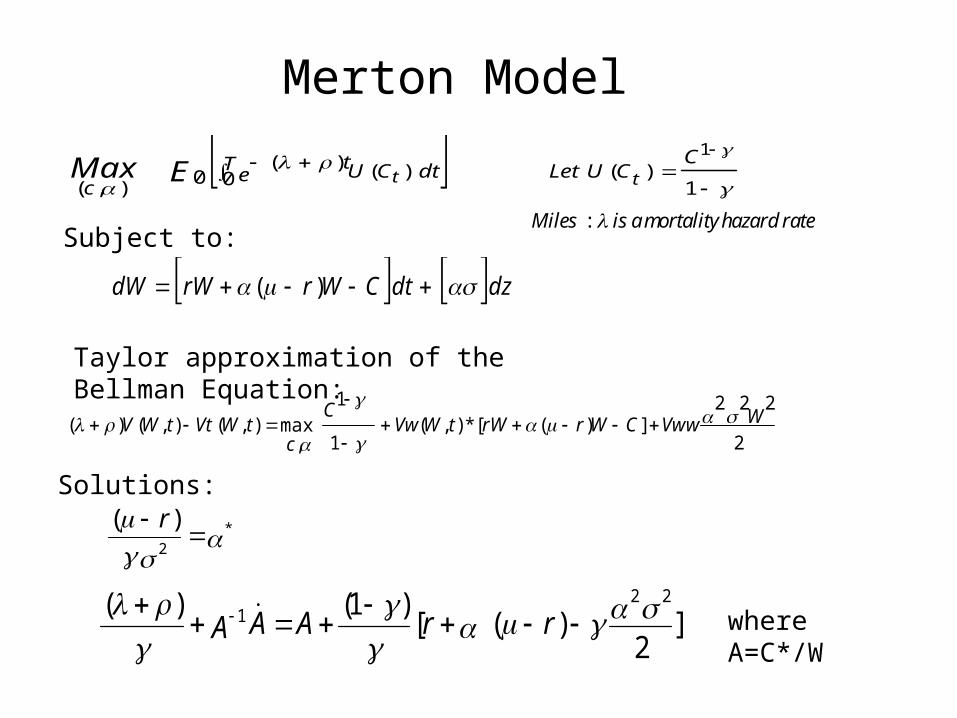
Merton Model

Subject to:

1)()(0

)(0

),(

1CCULetdtCUT

et

c ttEMax

dzdtCWrrWdW )(

2

222])([*),(

1

1max

,),(),()( WVwwCWrrWtWVw

C

ctWVttWV

Taylor approximation of the Bellman Equation:

Solutions:

*2

)(

r

]2

)([)1()( 22

1

rrAAA where A=C*/W

:Miles is amortality hazard rate

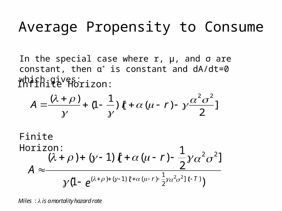
Average Propensity to Consume

Infinite Horizon:

]2

)()[1

1()( 22

rrA

)1(

]21

)()[1()(

)](2

1)()[1()(

22

22

e

rrA

Ttrr

In the special case where r, μ, and σ are constant, then α* is constant and dA/dt=0 which gives:

Finite Horizon:

:Miles is amortality hazard rate

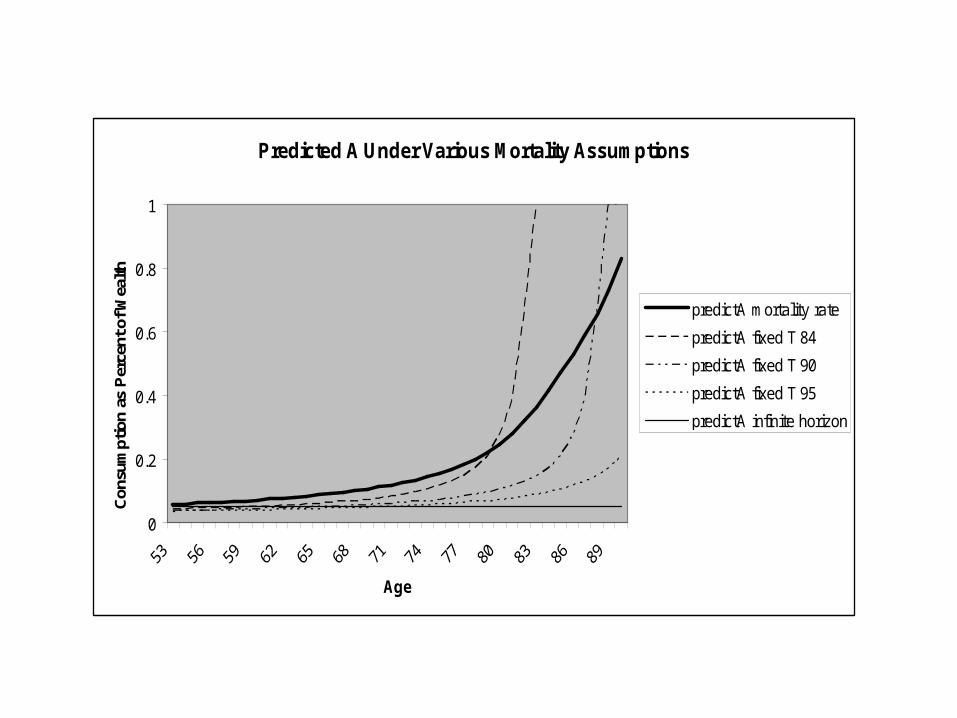
Predicted A Under Various Mortality Assumptions

0

0.2

0.4

0.6

0.8

1

Age

Con

sum

ptio

n as

Per

cent

of W

ealth

predictA mortality rate

predictA fixed T 84

predictA fixed T 90

predictA fixed T 95

predictA infinite horizon

Previous Paper Findings

Simple Merton model has very little ability to predict actual C/W using representative agent values for time preference and risk aversion

Solving the Merton equation for the time preference parameter and using the actual survey value for C/W generates an implied distribution for the time preference parameter that compares well to other distribution estimates (Samwick 1996; Barsky et al 1997)

C/W does co-vary as expected with model enhancements such as subjective mortality (life expectancy) and bequests

Covariates of A

• Previous paper: subjective survival expectancy; health; expected bequests (see Table 1)

• New demographics: (some shown Table 1)– Female financial respondent– Divorce & widowhood (remove divorced households

because not capturing wealth transfer from male to female)

– Retirement status (not shown – small negative coefficient)

– Education dummies (not shown, lower education has positive & significant coefficients)

– Race (not shown, nonwhite has sizeable positive coefficient)

Table 1Ln(A) (1) (2) Incl educ & race

Age of Head -0.016**

(-6.3)

-0.022**

(-8.0)

Ratio of Subjective Survival Probability to Actual Probability -0.063*

(-1.7)

-0.005

(-0.1)

Excellent/Very Good Health -0.076**

(-2.2)

-0.111**

(-3.2)

Fair/Poor Health 0.079*

(1.8)

0.006

(0.1)

Expect to Leave Any Bequest -0.242**

(-4.7)

-0.182**

(-3.2)

>50% Change of Leaving Bequest >$100,000 -0.316**

(-9.9)

-0.234**

(-6.6)

Female Financial Respondent 0.057

(1.4)

Widowed 0.166

(1.6)

Divorced -0.144**

(-2.1)

Female Widowed 0.174

(1.5)

Female Divorced 0.501**

(5.8)

R2 0.14 0.25

N 1,737 1,737

Explaining Distribution of C/W

My hypothesis generated by the 1st paper was that much of the variation in A, which is not well explained by Merton, may be heterogeneous preferences and/or, for the bottom group, an inability to plan or form expectations

Heterogeneous Preferences: Time & Risk Aversion (EIS – not currently separated) Correlate two distinct measures of preference Directly test explanatory power of survey measures and related

questions

Cognition, Expectation Formation & Planning Directly test survey measures

• Numeracy • Word recall• Precision of expectation formation• Planning Horizon

Two Residuals Containing Preferences:Wealth Residuals and Post-

Merton C/W Wealth residuals a la Hurst’s “Ants and Grasshoppers” (2004)

Residual after regressing financial wealth on income path, employment/health shocks, demographics (“opportunities to save”) – residual accumulated wealth is a variable that reflects past choices, independent of future shocks, should primarily reflect preferences

Ft-1 =f(Yh, rh, Ch, γ,ρ)

If consumption adjusts quickly, then C/W should be independent of past shocks. After accounting for age, expected returns, life expectancy , and bequests, under the Merton model, the residual should primarily reflect preferences

C/W=f(E[μ], r, age, γ,ρ, bequests) If both statements are accurate then the wealth residuals (from a

previous wave to minimize measurement error correlation) should be highly correlated with the residual of C/W as described above

Calculating Wealth Residuals

• Regress previous period net worth on everything we have to predict wealth accumulation “opportunities to save”: quadratic in average income over previous 20 years (measured at 2 intervals); coefficient of variation of income; health shocks over previous 10 years; recent employment shocks; education; etc. – residual reflects unexplained propensity to save

• Use residual as independent variable to predict C/W controlling for bequests, life expectancy, etc.

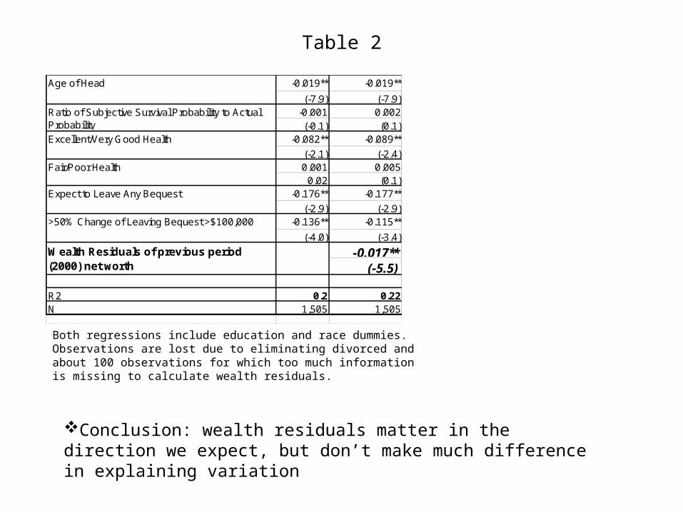
Table 2

-0.019** -0.019**

(-7.9) (-7.9)-0.001 0.002(-0.1) (0.1)

-0.082** -0.089**

(-2.1) (-2.4)0.001 0.005

0.02 (0.1)-0.176** -0.177**

(-2.9) (-2.9)-0.136** -0.115**

(-4.0) (-3.4)

-0.017**(-5.5)

R2 0.2 0.22N 1,505 1,505

Age of Head

Ratio of Subjective Survival Probability to Actual Probability

Excellent/Very Good Health

Fair/Poor Health

Expect to Leave Any Bequest

>50% Change of Leaving Bequest >$100,000

Wealth Residuals of previous period (2000) net worth

Both regressions include education and race dummies. Observations are lost due to eliminating divorced and about 100 observations for which too much information is missing to calculate wealth residuals.

Conclusion: wealth residuals matter in the direction we expect, but don’t make much difference in explaining variation

Table 3 Preference & Cognition MeasuresLn(A) (1) (2)

Risk Aversion Dummy – Highest Risk Aversion Category -0.03

(-1.1)

Preventative Health Measures 0.037

(0.8)

Smoke Ever 0.048*

(1.9)

Smoke Now -0.084**

(2.9)

Index of Precision of Expectations (Fraction of Exact Answers) -0.035

‘(-0.1)

Numeracy – Subtraction Easiest -0.105*

‘(-1.7)

Numeracy – Subtraction Hardest -0.076**

‘(2.4)

High Word Recall Dummy -0.089**

‘(-2.4)

R2 0.24 0.24

N 1,609 1,609

All regressions include demographics, life expectancy, bequests, etc. as above

Conclusion: Results Not Striking

Problem: Level of Wealth Highly Correlated

Ln(A) (1) (2)

Previous Reg with demographics, bequest, health, life, cognition

and preference variables

Add wealth quartiles

2nd Wealth Quartile -0.582**

(-17.4)

3rd Wealth Quartile -1.001**

(-27.7)

4th Wealth Quartile -1.461**

(-35.7)

R2 0.24 0.58

Other Preference/Planning Measures

• The HRS question about financial planning horizon (not shown in table) has a significant negative coefficient. Those with longer planning horizons have lower C/W

• I haven’t yet tried to use other direct measures of preferences and planning (other than risk aversion) from the experimental modules because sample size would be so low (1/2 or less or original module sample size).

• Perhaps trying to measure preferences (at least directly) and cognition is not the best question to ask here.

• At the least, the correlation between level of wealth and C/W potentially skews the answers to these measures→ Have to deal with wealth correlation to answer anything correctly

• Broadening the scope and/or thinking about confounding issues:

List (Questions & Preliminary Results) Fungibility/Liquidity: How does consumption relate to fraction of W in

current versus future assets Fraction of wealth in current assets has significant positive association

with C/W. But counter-intuitively, much of that is from positive coefficient on high fraction of wealth in housing

Pensions: Some studies suggest that, rather than being a substitute for pre-retirement asset accumulation, people with pensions save as much or more than people without pensions (back to preferences?) Dummy for anyDB plan significantly negative, as is value of DB (DC

negative but not significant)

Wealth: Do the rich save more?Possible reasons for co-variance of C/W with level of W Measurement error Preferences: high savers=high wealth & low C Incomplete adjustment to shocks Wealth sources riskier for wealthier?

Modeling Considerations

Within Model CRRA doesn’t allow risk/EIS variation by wealth

– Use HARA?? Separate Risk & EIS: Epstein-Zin/Kreps-Porteus

preferences

Specifying alternative such as “mental accounting”, myopia, or hyperbolic discounting??