AVC89: Rigid Velocities Compatible with

Five Image Velocity Vectors

SJ May bank

Hirst Research Centre

East Lane, Wembley, Middlesex HA9 7PP, UK

tions yield two quartic polynomial constraints, gi(v)= 52(v) = 0, on the translational velocity, v, of therigid body. We show that gi(v) and ?2(v) have, in gen-eral, exactly 16 distinct common zeros, and we showthat, in general, ten of these common zeros yield valuesof v compatible with the 2D motion field. An alterna-tive proof that there are ten values of v, based on thetheory of ambiguous surfaces, is sketched. Finally somequestions are raised concerning the connections betweenthe theory of image velocities and the theory of imagedisplacements.

The problem of obtaining rigid velocities compatiblewith a given set of image velocity vectors is algebraic inthat it depends on the solution of simultaneous polyno-mial equations. We show that five image velocity vectorsyield two quartic polynomial constraints on the transla-tional part of the rigid velocity, and that of the 16 com-mon zeros of these two quariics, exactly ten yield rigidvelocities compatible with the image velocities. An al-ternative argument that there are in general exactly tenrigid velocities compatible with five given image veloci-ties is briefly sketched.

The fact that as many as ten rigid velocities are ob-tained indicates that the problem of finding rigid veloci-ties compatible with image velocities is intrinsically dif-ficult.

A body moving relative to a camera gives rise toan image that changes over time. These image changesare described by a 2D motion field of velocity vectorsdefined on the projection surface of the camera [1,2,3].Information about the motion and shape of the bodycan be obtained from the 2D motion field. In particular,if the 2D motion field arises from a single rigid movingbody, then it can yield the shape and velocity of thebody up to a single unknown scale factor [1,2,3,4].

The problem of recovering the shape and velocityof a rigid body from the associated 2D motion field isalgebraic, because it depends on solving a number ofsimultaneous polynomial equations. We investigate theproperties of these equations, and show that there are,in general, exactly ten rigid velocities compatible witha given 2D motion field containing five image velocityvectors. The figure ten in this context is a fundamentalmeasure of the complexity of the problem of recoveringrigid body motion from image velocities, analogous tothe degree of an algebraic curve. Ten is considered high,indicating that the problem is difficult.

The phrase 'in general' means that although some2D motion fields containing five image velocity vectorsare not compatible with exactly ten rigid velocities, such2D motion fields form a negligibly small part of thespace of all 2D motion fields containing five image ve-locity vectors.

We describe some general properties of polynomialsand then obtain the equations for the 2D motion fieldarising from a single moving rigid body. These equa-

POLYNOMIALS

We use TZn to denote n-dimensional Euclidean space,and Vn to denote n-dimensional projective space. Thepoints of Vn are represented by n + 1-tuples of coordi-nates such that at least one coordinate is non-zero. Twopoints x, y of Vn with coordinates a;,-, y,- are identifiedif and only if there exists a non-zero scalar A such thatXi = Xyi for 1 < i < n + 1.

Let x = (x\,X2,X3). A polynomial /(x), homoge-neous in the coordinates of x, defines a plane curve inV2. A point u is on /(x) if and only if /(u) = 0. Leth = V/(x)|u = (df/dxu df/dx2, df/dx3) evaluatedat u. A point y is on the tangent line to /(x) at uif and only if h.y = 0. If h = 0 then /(x) is said tohave a singular point at u. The condition that /(x)has a singular point somewhere in V2 is expressible asa polynomial constraint on the coefficients of /(x).

Plane curves /(x), g(x) are said to intersect transver-sly at u if /(u) = g(u) = 0 and V/(u) x V#(u) ^ 0.Transverse intersections are stable, in that if/(x), g(x)are subject to small perturbations then the perturbedpolynomials intersect transversely at a point near to u.

Plane curves /(x), g(x) of degrees m, n respectively,intersect at mn points, and these points are distinct ifand only if each intersection is transverse. If /(u) =</(u) — 0, but /(x), g(x) do not intersect transverselyat u then /(x), g(x) are said to have a multiple commonzero at u.

A property defined on Vn holds in general if it holdson an open dense set of Vn. If a polynomial is non-zeroat just one point of Vn then it is non-zero on an opendense set of Vn, thus a polynomial defined on V" iseither identically zero or it is in general non-zero.

Further information on polynomials, curves and pro-

199AVC 1989 doi:10.5244/C.3.34

jective spaces is given in [5].

2D MOTION FIELDS

The 2D motion field is defined to be the projection of thethree dimensional velocity of a body onto the projectionsurface of the camera [1,2]. The velocity of a point onthe body surface projects to an image velocity vector,Qi, and the point itself projects to the base point, Qi,of Q,-. We assume that the body is rigid, and we assumethat the image is formed by polar projection onto theunit sphere, centred at the projection point.

The velocity of a rigid body in space is describedby a translational velocity v, and an angular velocityO. (See [6]). The axis of fl is chosen to pass throughthe centre of the projection sphere. With this choice ofaxis, v, fl are uniquely determined by the motion of therigid body.

The main equations

The image velocity vectors, Q,-, with base points, Q,-,are related to v, ft as follows [1,2,3,4]

Q, = [v - (v.Q,-)Q<]#< + f i x Q j (1)

where Ki is the inverse distance to the rigid body sur-face in the direction Q,-. A value of v is said to becompatible with the 2D motion field if there exist asso-ciated values of il and Ki such that (1) holds.

It follows from (1) that v — 0 is, in general, notcompatible with the 2D motion field because the Q,-would otherwise be coplanar. As we only consider thegeneral case, we assume v ^ 0. If v ^ 0 is compatiblewith (1) then Av is compatible with (1) for any A ^ 0.It is thus natural to regard v as an element of V2.

Define Rj by R, = Q,- x Q,-. On taking the dotproduct of (1) with Qi x v, we eliminate Ki to obtain

The R,-, Q, are known quantities obtainable from theimage, and v, fl are unknown quantities, to be deter-mined by solving (2). Our main result is that if fivepairs Qi, Q,- are given then there are exactly ten valuesof v satisfy (2), and hence satisfy (1). We assume fromnow on that 1 < i < 5.

On taking the scalar product of (3) with Q,- we obtaina»v.Qi + bi = 0, thus

Qi = [v — (v.Qi)Qi]di + ft x Q, (4)

Equation (1) follows from (4) on setting Ki = ai.

We complete the proof by showing that v x Qj ̂ 0for all i. If, for example, v x Q5 = 0, then without lossof generality, v = Q5. We write the first four equationsof (2) in the matrix form r(v) = M(v)ft. As fi variesover 7£3, M(Q5)fi varies over a subspace 5 of TZA ofdimension at most three. If (2) has a solution with v =Q5 then S includes r(Qs), however, r(Qs) varies overthe whole of H4 as the R, vary, thus r(Q5) = M(Q5)fldoes not, in general, have a solution for ft.

Properties of (v.Q,)Q, — v

We require the following two results: if v varies, withthe Qi fixed and in general position then (i) no three ofthe vectors (v.Q,)Qi — v are ever collinear; and (ii) thefive vectors (v.Q,)Qi — v always span TZ3. The proofsare omitted.

Define cubic polynomials /ijfc(v) by

= det'(v.Q.-)Qi-v(v.Qj)Qj-v (5)

where 1 < i < j < k < 5. We show that the /,jfc(v) donot, in general, possess a singular point.

The /ijjt(v) form a family of polynomials indexedby the components of Qi,Qj,Qjt- The condition thatfijk(v) possess a singular point can be expressed as apolynomial constraint on the coefficients of /,jjt(v), andhence as a polynomial constraint c(Q,-, Qj, Q*) = 0 onQi, Qj, Q,t Either c(Q*, Qj, Q*) = 0 for all Q,-, Q;-, Qk

or c(Q,-, Qj-, Qjt) 7̂ 0 in general, thus it suffices to findjust one triple Q.,Q;,Qi for which c(Qj,Qj,Qfc) ^0, or equivalently for which /,jj;(v) does not possess asingular point. To this end, select

Qk = (0,0,1)

On substituting the above values of Qi, Qj,(5), we obtain

into

No solutions are lost

We show that we do not overlook any solutions to (1) bypassing to (2). In other words, we show that if v ̂ 0 iscompatible with (2) then O, Ki can be found such that(1) holds. We obtain from (2)

Let v x Qsuch that

( Q i - n x Q,).(v x Qi) = 0

0 for all i. Then there exist scalars a,-, &,•

Qi = a,v + 6iQi + f lx Q, (3)

v/3fijk(v) = ^ -

1+ v3v

22 + - - vf)]

It can be shown that V/,-jfc(v) ^ 0 for all v, thus /ijjt(v)does not possess a singular point for the three specifiedvalues of Qi, Qj, Qt, thus fijk(v) does not possess asingular point in general.

Two quartic polynomials

The condition that the first four equations of (2) becompatible with a single value of ft yields the quartic

200

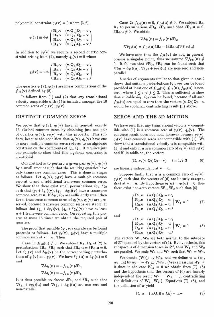
polynomial constraint gi(v) = 0 where [3,6].

\R4.v (v .Q 4 )Q 4 -v ,

In addition to gi(v) we require a second quartic con-straint arising from (2), namely q2(v) = 0 where

Ri.v ( v . Q i ) Q i - v '

!a-v (v .Q 3 )Q 3 -v•R 5 v (v .Q 5 )Q 6 -v ,

The quartics 9i(v), q2(v) are linear combinations of thefijk(v) defined by (5).

It follows from (1) and (2) that any translationalvelocity compatible with (1) is included amongst the 16common zeros of qt (v), <?2(v).

Case 2: /i23(u) = 0, /i24(u) ^ 0. We subject R3,R5 to perturbations 6H3, 6R5 such that 6R3.U = 0,6K5.u # 0. We obtain

= /i25(u)<5R3 - (<5R5.u)V/i23(u)

We have seen that the fijk{v) do not, in general,possess a singular point, thus we assume V/123(u) 7̂0. It follows that 6R3, 5R5 can be found such thatV(<?i + 5?i)(u), V(?2 + £g2)(u) are non-zero and non-parallel.

A series of arguments similar to that given in case 2shows that suitable perturbations 6q\, 8q2 can be foundprovided at least one of /i23(u), /<j4(u), /tjs(u) is non-zero, where 1 < i < j < 3. This is sufficient to showthat suitable 8qi, Sq2 can be found, because if all such/,j/t(u) are equal to zero then the vectors (u.Q,)Q, — uwould be coplanar, contradicting result (ii) above.

DISTINCT COMMON ZEROS

We prove that <7i(v), ?2(v) have, in general, exactly16 distinct common zeros by obtaining just one pairof quartics 91 (v), g2 (

v) with this property. This suf-fices, because the condition that <?i(v), g2(v) have oneor more multiple common zeros reduces to an algebraicconstraint on the coefficients of Q;, Q,-. It requires justone example to show that this algebraic constraint isnon-trivial.

Our method is to perturb a given pair q\ (v), ?2(v)by a small amount such that the resulting quartics haveonly transverse common zeros. This is done in stagesas follows. Let 9i(v), g2(v) have a multiple commonzero at u and n additional transverse common zeros.We show that there exist small perturbations 6q\, Sq2such that (31 + 6qi)(v), (q2 + 8q2)(v) have a transversecommon zero at u. If 6qi, 6q2 are sufficiently small thenthe n transverse common zeros of qi (v), g2(v) are pre-served, because transverse common zeros are stable. Itfollows that (qi + 8qi)(v), (32 + <$<Z2)(v) have at leastn + 1 transverse common zeros. On repeating this pro-cess at most 15 times we obtain the required pair ofquartics.

The proof that suitable 8qi, 6q2 can always be foundproceeds as follows. Let 5fi(v), <72(v) have a multiplecommon zero at v = u. Then

Case 1: /i23(u) ^ 0. We subject R4, R5 of (2) toperturbations 6R4, 6R5 such that i5R4.u = 6R5.U = 0.Let 8qi(v) and <$g2(v) be the corresponding perturba-tions of ?i(v) and g2(v). We have <5gi(u) = 6g2(u) = 0and

u) = -/i23(u)<5R4

It is thus possible to choose 6K4 and <5R5 such thatV(qi + Sqi)(u) and V(q>2 + ̂ ?2)(u) a r e non-zero andnon-parallel.

ZEROS AND THE 3D MOTION

We have seen that any translational velocity v compat-ible with (1) is a common zero of gi(v), g2(v). Theconverse result does not hold however because <7i(v),g2(v) have common zeros not compatible with (1). Weshow that a translational velocity u is compatible with(1) if and only if u is a common zero of qi(v) and g2(v)and if, in addition, the vectors

(R,-.v,(v.Q i)Q,-v) 1 = 1,2,3 (6)

are linearly independent at v = u.

Suppose firstly that u is a common zero of <h(v),g2(v) such that the vectors of (6) are linearly indepen-dent at v = u. By hypothesis gi(u) = g2(u) = 0, thusthere exist non-zero vectors Wj, W2 such that [6]

fRj.u (u.QOQi-iiR2.u (u.Q2)Q2 — uR3.u (u .Q 3 )Q 3 -u

vR4.u (u.Q4)Q4 — u>

(7)

andLiu (u.Q1)Q1-u>

R2.u (u.Q2)Q2 — uR3.u (u .Q 3 )Q 3 -u

.R5.u (u.Q5)Q5 — u,The vectors Wj, W2 are both normal to the subspaceof 7£4 spanned by the vectors of (6). By hypothesis, thissubspace is of dimension three in 7Z.4, thus Wi and W2

are parallel. We scale Wi and W2 such that Wi = W2.

We denote (W;)j by Wij, and we define w = [w\,w2, W3) by Wj = —W\ j+i/Wii. (We can assume W\\ ^0 since in the case W\\ = 0 we obtain from (7), (8)and the hypothesis that the vectors of (6) are linearlyindependent the result Wj = W2 — 0, contradictingthe definitions of Wi, W2.) Equations (7), (8), andthe definition of w yield

201

It follows from (9) that v = u, fl — w is a rigid velocitycompatible with (1).

Next, suppose that u is a common zero of <h(v),92 (v) such that the three vectors of (6) are linearly de-pendent. We show that u is in general not a transla-tional velocity compatible with the 2D motion field.

It follows from our hypothesis concerning u that thevectors (u.Q,-)Q;—u, i = 1,2,3 are contained in a singleplane II. The vectors (u.Qi)Q* — u (1 < i < 5) spanTZ3, thus at least one of (u.Q4)Q4 — u, (u.Q5)Qs - uis not contained in II. It follows that R4, R5 and Q4,Qs can be chosen such that

det

R4.11 (u.Qi)Qi-u>R2.U (u.Q2)Q2 — uR 4 u (u.Q4)Q4 - u

5.u (u.Q5)Q5-u>

The choice of R4, R5 and Q4, Q5 does not affect thecondition qi(u) = 92(1) — 0, since we are assuming thatthe vectors of (6) are linearly dependent. It follows thatu is in general not compatible with (2).

THE MAIN RESULT

We have seen that a possible translational velocity v iscompatible with the 2D motion field if and only if v isa common zero of 9i(v), 32(v) such that the vectors of(6) are linearly independent, and we have shown that3i(v), <Z2(v) have 16 distinct common zeros. We nowshow that there are exactly six values of v such that thevectors of (6) are linearly dependent. The main resultthat there are, in general, exactly 10 = 16-6 values of vcompatible with a 2D motion field containing just fiveflow vectors then follows.

Define the matrix A by

A= (v .Q 2 )Q 2 -v =(v .Q 3 )Q 3 -v

where the At are 3 x 3 matrices with coefficients inde-pendent of v. Let g(v) = det(Aiv\A2v\A3v). We recallthat the row rank of a matrix is equal to the columnrank of a matrix. The rows of A are linearly dependentif and only if v satisfies both

</(v) = /i23(v) = 0 (10)

and0 (11)

There are at most nine distinct values of v satisfying(10) because g(v), /i23(v) are cubic plane curves, andamongst these there are at most three distinct values ofv, corresponding to the roots of the eigenvalue equation

det(vl2 - Ai43) = 0

for which (11) fails to hold.

Direct calculation reveals that there are in generalexactly three distinct values of v for which A2Y x A3V =

0. (To simplify matters, coordinates can be chosen suchthat Qi = (1,0,0) and (Q2)3 = 0.) It is thus sufficientto show that there are, in general, exactly nine values ofv satisfying (10), and for this it is sufficient to produce asingle example for which there are nine distinct values ofv satisfying (10). The example is constructed as follows.

Set Ri = R2 = 0. Then the first two rows of A arelinearly dependent if and only if v = Qi, Q2 or Qj x Q2

(as points of V2). Suppose that v is not equal to Qi,Q2 or Qi x Q2. In this case (with Ri = R2 = 0) therows of A are linearly dependent if and only if

R3.v = 0 and /i2s(v) = 0 (12)

There are, in general, exactly three values of v satisfying(12), because R3.V = 0 is a linear constraint on v and/i23(v) = 0 is a cubic constraint on v. In general Qi,Q2, Qi x Q2 are not on the line R3.V = 0, thus weobtain a total of six distinct values of v for which therows of A are linearly dependent, and these six valuesof v satisfy (10).

It follows that if Ri = R2 = 0 then there are exactly9 = 6 + 3 distinct values of v satisfying (10), thus thereare, in general, exactly nine distinct values of v satisfy-ing (10), hence there are, in general, exactly six valuesof v for which the rows of A are linearly independent.

AN ALTERNATIVE METHOD

The above proof that there are, in general, exactly tendistinct rigid velocities compatible with five given imagevelocities is closely tied to the image plane. A sketchof an alternative proof of the same result is now givenbased on constructions in 3D space and the theory ofambiguous surfaces [3,4].

We recall from [4] that if points P in space movingrigidly with velocity v, fl give rise to image velocitiesthat are also compatible with a second rigid velocity v',fl' then the points P lie on the quadric surface

l.P = (W'.P)(v'.P) - (W'.v')(P.P) (13)

where 1 = v' x v and W = ft - fl'. Equation (13) canbe written in the form

PMP = 0 (14)

where M is a symmetric matrix and 1 is a vector satis-fying l.v = 0.

Let five image velocities Q, with base points Qj begiven, together with a single compatible rigid velocityv, fl. Then we can construct points P,- in space withvelocities P, = v + fl x P, such that P, projects toQi and P, projects to Qj. Let S be the space of allquadrics of the form (14) that contain the five points P,.The quadrics of 5 are subject to six linear constraints,namely, l.v = 0 and

202

thus S has dimension two and hence S is a copy of V2

embedded in the space of all quadrics. Each rigid ve-locity v', ft' distinct from v, ft but compatible withthe Qj, Q,- yields a quadric in S with an equation ofthe form (13). Thus, in order to count the rigid veloci-ties compatible with the Q,-, Qt- it suffices to count thequadrics in S of the form (13).

Let ip be the element of S specified by a pair M, 1,and define the matrix N by

N = M - -TiSice(M)I

The quadric ij> has an equation of the form (13) for somechoice of v', W if and only if

det(JV) = 0 and 17V1 = 0 (15)

The equations of (15) define two cubic curves in S whichintersect at nine points. We thus obtain 10 = 9+1 rigidvelocities compatible with the five image velocities Q,.

CONCLUSION

We have shown that there are, in general, exactly tenrigid velocities compatible with a 2D motion field con-taining five image velocity vectors. Ten is thus a basicmeasure of the complexity of the problem of obtainingrigid velocities from 2D motion fields. In this contextten is high, indicating that the problem is intrinsicallydifficult.

Some of the ten rigid velocities may have complexcoordinates, in which case they can be discarded onphysical grounds. It may also be possible to discardrigid velocities not yielding feasible positions for thepoints on the rigid body surface giving rise to the 2Dmotion field, in that some of the points are behind thecamera. An example of ten rigid velocities compatiblewith five image velocity vectors is obtained in [7] usingthe REDUCE computer algebra system.

An image velocity field can be regarded as the limitof a sequence of image displacement fields, as the sizeof the displacement becomes small. As a result it ap-pears that many of the properties of image velocitiesmay carry over to the more complicated case of imagedisplacements. For example, a) Demazure [8] showsthat there are, in general, exactly ten rigid displace-ments compatible with five given image displacements;b) the two classes of ambiguous surfaces associated withimage displacements and image velocities, respectively,happen to coincide; and c) the ambiguous surfaces aris-ing from image displacements are subject to two cubicconstraints analogous to those quoted in (15) above [9].

Questions about the possible connections betweenthe theories of image displacements and image velocitiesnow arise. For example, let Si be a sequence of five pointimage displacement fields such that Si —* S where cS isan image velocity field. Let % be the set of ten rigiddisplacements compatible with Si and let T be the setof ten rigid displacements compatible with S. Then isit the case that % -* T ?

It is known that there exist five point image displace-ment fields compatible with ten real rigid displacements,of which three are feasible [10], however Horn [11] hascarried out experiments indicating that many five pointimage displacement fields are compatible with exactlyfour real rigid displacements, only one of which is fea-sible. It may be possible to obtain some understandingof these results by studying the simpler case of imagevelocities.

ACKNOWLEDGEMENTS. This work was carriedout at Marconi Command and Control Systems Ltd.,Frimley as part of ESPRIT Project P940. The authorgreatfully acknowledges discussions with C.H. Longuet-Higgins.

REFERENCES

1. Horn, B.K.P. Robot Vision. MIT Press (1986).

2. Longuet-Higgins, C.H. and Prazdny, K."The interpretation of a moving retinal image".Proc. Roy. Soc. Lond. B Vol. 208 (1980) pp385-397.

3. Maybank, S.J. A theoretical study of optical flow.PhD Thesis, Birkbeck College, University of Lon-don (1987).

4. Maybank, S.J. "The angular velocity associatedwith the optical flow field arising from motionthrough a rigid environment". Proc. Roy. Soc.Lond. A Vol. 401 (1985), pp 317-326.

5. Walker, R. Algebraic Curves. Dover, New York(1962).

6. Sokolnikoff, I.S. and Redheffer, R.M. Math-ematics of Physics and Modern Engineering. Mc-Graw-Hill (1966).

7. Trivedi, H.P. "On computing all solutions to themotion estimation problem with exact or noisydata". Submitted to Comp. Vision., Graphicsand Image Process. (1989).

8. Demazure, M. "Sur deux problemes de recon-struction". INRIA Rapports de Recherche No.882 (1988).

9. Maybank, S.J. "The Projective geometry of am-biguous surfaces." MCCS Report T(S)T/2012(1989).

10. Faugeras, O.D. and Maybank, S.J. "Motionfrom point matches: multiplicity of solutions".IEEE Workshop on Computer Vision, Irvine, Cal-ifornia, USA (1989) pp 248-255.

11. Horn, B.K.P. "Relative orientation". Acceptedfor publication by the Int. J. Comp. Vision (1989).

203