available copy - dtic · dbms's include structure query language (sql) and query by example...
TRANSCRIPT

BestAvailable
Copy

NAVAL POSTGRADUATE SCHOOLMonterey, California
AD-A280 415SDTI C
ELL,ýc-r~zfl
V QUALITY INSPEDS
THESIS
THE COMPARISON OF SQL, QBE, AND DFQLAS QUERY LANGUAGES
FORRELATIONAL DATABASES
by
Panmtungan Girsang
March 1994
Thesis Advisor. C. Thomas Wu
Approved for public release; distribution is unlimited.
94 6 20 008 94-18941
Form Appme
REPORT DOCUMENTATION PAGE oUB No. 070"IU
PWPubbo eum1hed. o -u -ds atm "dna. isues to IQ 1 how W pet"W"gn. Miom"li doe 1Wf reWAWig Isbmwo, SdIi snaw" do Smawa=g A a mm do.I di d ied, ad amaher addta m . O e.W oofa moorn~mo. Swe comed. i #ws' eawnwe or aw adi mp" o fts
ain i immed, maggeasm d d em t W Heewt quut $emom, Overa. tr h & Oprapsm.wwaidAegm. 1215 sd....Osis N w, Sub. t 5 Aiboimm, VA 0 aid i lme�d � �Ma d ,d bidgi, Pe l Aeduaame Pr i (O7I.o1N, Wa , aqi.n. C
1. AE[NY USE ONLY (Leve @Ink) P. REPORT DATE I REPNT AM DATES COVENFO
i March 1994 Master's Thesi:.TIPTLE AND SUBTITLE L. FUNDING NUMBERS
The Comparison of SQL, DFQL, and DFQL as Query Languagesfor Relational Databases
L AUTHOR(S)
Girsang, Paruntungan
7. PERFORMING ORGANIZATION NAME(S) AND ADDRESSMS) It PERFORMING ORGANIZATIONNaval Postgraduate School REPORT NUMBER
Monterey, CA 93943-5000
IL SPONSORONG MONITORING AGENCY NAMEMS AND ADDRESSWE) IQ. SPONSORING MONITORISGAGENCY REOfrT NUMBER
11. SUPPLEMENTARY NOTES
The views expressed in this thesis are those of the author and do not reflect the official policy or positionof the Department of Defense or the United States Govemmtt.
12L. DISTRIUTION I AVAWLAUTY STATEMENT m DTRBUTICODEApproved for public release; distribution is unlimited.
1& ABSTRACT (Phxhrn 2 ad mns)Structure Query Language (SQL) and Query By Example (QBE) are the most widely used query
languages for Relational Database Management Systems (RDBMS's). However, both of them haveproblems concerning ease-of-use issues, especially in expressing universal quantification, specifyingcomplex nested queries, and flexibility and consistency in specifying queries with respect to data retrieval.To alleviate these problems, a new query language called "'Datalow Query Language" (DFQL) wasproposed.
This thesis investigates dhe relative strengths and weaknesses of these three languages. We dividequeries into four categories: single-value, set-value, statistical result, and set-count value. In eachcategory, a representative set of queries from each language is specified and compared. Some of thequeries specified are logical extensions of the other (already defined) queries, which are used to analyzethe query languages' flexibility and consistency in formulating logically related queries. We perform asimple experiment of asking NPS CS students to write a small set of queries in all three languages.
Based on the analysis, we conclude that DFQL eliminates the problems of SQL and QBE mentionedabove. The relative strengths of DFQL comes mainly from its strict adherence to relational algebra anddataflow-based visuality.
14. SUBJECT TERMS 1. NMt"BER OF PAGESSQL, QBE, DFQL, Relational Model, Database Management Systems, 142Flexibility, Ease-of-use, Consistency. s. "iA
.URITYQLAGTIO 1. IU SECIRITTVLABI.NFAIM It SECURITY CLASUCATM 2L. UMMATION OF ABSTRACTOF liPlRT OPTMNPAGE OF ASRCUOnPssified Unclassified lUnclassified ULUnclassicledsifieU
NSN 7540.01-280-5500 Stuidad Farm 298 (Rav. 2-89)i mmabo by AMRSI. 239-LI

Approved for public release; distribution is unlimited
THE COMPARISON OF SQLj, QBE, AND DFQLAS QUERY LANGUAGES
FOR RELATIONAL DATABASES
by
Paruntungan GirsangLieutenantý Indonesian Navy
B.S., University of North Sumnatera, Indonesia, 1981Ir., University of North Sumatera, Indonesia, 1983
Submitted in partial. fulfillment of the
requremntsfor the degree of
MASTER OF SCIENCE IN COMPUTER SCIENCE
from the
NAVAL POSTGRADUATE SCHOOL
March 1994
Author.____
Prnmgan Girsang
Approved By:
Department of Computer Science
ti
ABSTRACT
Structure Query Language (SQL) and Query By Example (QBE) are the most widely
used query languages for Relational Database Management Systems (RDBMS's).
However, both of them have problems concerning ease-of-use issues, especially in
expressing universal quantification, specifying complex nested queries, and flexibility and
consistency in specifying queries with respect to data retrieval. To alleviate these problems,
a new query language called "DataFlow Query Language" (DFQL) was proposed.
This thesis investigates the relative strengths and weaknesses of these three languages.
We divide queries into four categories: single-value, set-value, statistical result, and set-
count value. In each category, a representative set of queries from each language is
specified and compared. Some of the queries specified are logical extensions of the other(already defined) queres, which are used to analyze the query languages' flexibility and
consistency in formulating logically related queries. We perform a simple experiment of
asking NPS CS students to write a small set of queres in all three languages.
Based on the analysis, we conclude that DFQL eliminates the problems of SQL and
QBE mentioned above. The relative strengths of DFQL comes mainly from its strict
adherence to relational algebra and dataflow-based visuality.
Aoession For
OTIS GA&I 1DTIC TAB 0Utla"nunoced 03 Wu3t ifiation
ByAvo tiability Codes
A 6SD4W/6b
Din

TABLE OF CONTENTS
I. INTRODUCTION ..................................................................................................... 1A. BACKGROUND .............................................................................................. 1B. MOTIVATION .......................................................................................... 2
C. OBJECTIVE .............................................................................................. 3D. CHAPrER SUMMARY ... .. ......................................................................... 4
IL DESCRIPTON OF THE RELATIONAL MODEL AND QUERY LANGUAGES
FOR RDBMS's .......................................... 5
A. THE RELATIONAL MODEL CONCEPTS ............................................. 5
I. Fornal Terminology ...................................... 6
2. Propertes of Relation ..... . .................................... 8B. TEXT-BASED QUERY LANGUAGES ......................................... 8
1. The Relational Algebra ..................................... 82. The Relational Calculus ............................................. 10
3. Szuctuzr Query Language (SQL) ............................. 10
a. Data Definition in SQL ............ ................................... 11
b. Data a .......a..... ................................ 1..... 1
C. Logical Operators of SQL .............................. 13
d. The Problms withSQL ....................................................... 13(1) Declarative N ..at=............................... 14
(2) Universal Quantification ................. o .................... 15
(3) Lack of Orthogonality ............................................. 17(4) Nesting c onstuct..................................................... 17
C. VISUAL-BASED QUERY LANGUAGES ............................. 18
I. QBE, a Fonn-based Quey Language .............................................. 18
. Data Recieval ...... ..............................19
b. Built-in functions, Grouping and other Operators ..................... 20
c. The Problems with QBE E................................ 21
iv
2. Datalow Query Language (DFQL) ........................................... ......... 21a. DFQL Operators ......................................................................... 22
(1) Basic Operators ......................................................... 23(2) Other Primitives Operators ....................................... 26
(3) Display Operators ..................................................... 29(4) User-defined Operators ............................................. 29(5) DFQL Query Construction ....................................... 29
(6) Incremental Queries ................................................... 30(7) Universal Quantification .......................................... 30(8) Nesting and Functional Notation ............................... 31(9) Graph Structure of DFQL Query ............................... 31
3. Entity-Relationship Model Interface ............................................. 31
IlL THE COMPARISON OF SQL, QBE, AND DFQL WITH RESPECT TODATA RETRIEVAL CAPABILXIIES .......................................................... 34
A. CATEGORIES OF QUERY ................................................................... 35
I. Single-Value ................................................................................... 35a. Query 1: Simple retrieval .................................................. 36
b. Query 2: Qualified retrieval ................................................ 38
C. Query 3: Retrieval involves more than two tables ............. 40d. Query 4: Retrieval involving universal quantification ..... 42
e. Query 5: Retrieval involving a negation statement ........... 442. Set-Value ........................................................................................ 47
a. Query 6: Retrieval involving existential and universal
uantification......................................................................... 47b. Query 7: Retrieval involving explicit sets ......................... 49
C. Query 8: Retrieval involving explicit sets ......................... 51d. Query 9: Retrieval involving universal quantification ..... 54e. Query 10: Retrieval involving existential and universal
quantification........................................................................ 57f. Query 11: Retrieval involving set operation ........................ 59
V

3. Statistical Result ................................................................................... 62a. Query 12: Retrieval involving aggregate AVG function ....... 62
b. Query 13: Retrieval involving AVG and Groupnig function .... 64
C. Query 14: Retrieval involving Count, AVG, and Grouping
function ................................................................................ 66d. Query 15: Retrieval involving Count and AVG function ......... 68
e. Query 16: Retrieval involving Max and Grouping function ..... 70
f. Query 17: Retrieval involving Max and Grouping function ..... 72
g. Query 18: Retrieval involving Avg, Max, Sum, and Grouping
function ................................................................................ 74h. Query 19: Retrieval involving Count and Grouping function ...76
4. Set-Count Value ............................................................................. 79a. Query 20: Retrieval involving existential quantification ....... 79b. Query 21: Retrieval involving Count and Grouping function ...81c. Query 22: Retrieval involving Count and Grouping function ...84
d. Query 23: Retrieval involving Count function ..................... 87
e. Query 24: Retrieval involving universal quantification ..... 89f. Query 25: Retrieval involving universal quantification ..... 91
B. ANALYSL S ........................................................................................... 93I. Ease-of-use ..................................................................................... 93
a. Queries involving existential or universal quantification .......... 94
(1) SQL ......................................................................... 94(2) QBE ........................................................................... 95
(3) DFQL . ...................................................................... 95b. Queries involving nested queries ................................................ 96
(1) SQL ......................................................................... 96
(2) QBE ........................................................................... 96
(3) DFQL .............................................................................. 96
2 i ............................................................................................ 9
a. SQL ........................................................................................ 98b. QBE .................................................... ................................. 98
c. DFQL .................................................................................... 99

3. Consistency .......................................................................................... 99
a. SQ L ............................................................................................ 100
b. Q BE ........................................................................................... 100
c. DFQL ......................................................................................... 1004. Relative Strengths and Weaknesses ................................................... 101
IV. HUMAN FACTORS EXPERIMENT ............................ 11A. HUMAN FACTORS ANALYSIS OF QUERY LANGUAGES ..... 111
B. EXPERIMENTAL COMPARISON OF SQL, QBE, AND DFQL ... 111
1. Assesment of the Experiment .......................................................... 111
a. Subjects ................................... 112
b. Teaching Method ...................................................................... 112
C. Test Queries .............................................................................. 112
d. Evaluation Method ................................................................... 1132. Experiment Results ............................................................................. 114
3. Experiment Conclusion ...................................................................... 117
a. Query (Q1) ................................................................................ 117
b. Query (Q2) ...................................... 117
c. Query (Q3) ......................................... 117
d. Query (Q4) ................................ 118
d. Query (QS) .............................................................................. 118
V. CONCLUSIONS ................................................................................................... 120
LIST OF REFERENCES ........................................................................................... 122
APPENDIX A ......................................................... 125
INrTIAL DISTRIBUTION LIST ........................................ 128
vii

LIST OF TABLES
TABLE 2.1 BASIC DFQL OPERATORS AND THEIR SQL EQUIVALENTS .... 23
TABLE 2.2 NON-BASIC DFQL OPERATORS AND THEIR SQL EQU1BA-
LENTS .............................................................................................. 26
TABLE 3.1 RELATIVE STRENGTHS AND WEAKNESSES OF SQL, QBE,
AND DFQL ......................................................................................... 102
TABLE 4.1 EXPERIMENT RESULT ..................................................................... 115
TABLE 4.2 PERCENT CORRECT OF SUBJECT CLASSIFICATION FOR
QI, Q2, AND Q3 ................................................................................ 116
TABLE 4.3 PERCENT CORRECT OF SUBJECT CLASSIFICATION FOR Qi
THROUGH Q5 ................................................................................ 116
'Mii

LIST OF FIGURES
Figure 2.1 A Relation STUDENT Schema ......................................................... 7
Figure 2.2 Operator Construction ...................................................................... 22
Figure 2.3 ER-Diagram of the COMPANY database ....................................... 32
ix
LIST OF QUERIES
Query 2.1 Example of Relational Algebra Query ............................................... 9Query 2.2 Example of Relational Calculus Query ............................................ 10
Query 2.3 Example of SQL Query .................................................................. 16
Query 2.4 Example of QBE Query ................................................................... 19
x

ACKNOWLEDGEMENTS
I would like to thank the Indonesian Navy for the opportunity to study at the Naval
Postgraduate School (NPS) in Monterey, California.
I would like to thank Dr. C. Thomas Wu for his continued support, enthusiasm,
patience, and guidance. These were invaluable assets for the completion of this work. I
would also like to thank LCDR John S. Falby for his help and support in editing. His
assistance and direction were both enlightening and timely.
I wish to thank to Computer Science students at NPS who participated in a human
factors experiment. These support was instrumental in the completion of this thesis.
I am very grateful to my parents for their support and faith. Most importantly, I am
indebted to my wife Ediana, my daughter Jean Liatri Augustine and my son John Samuel
Sebastian, for their constant love, patience and understanding.
,ci

L INTRODUCTION
A. BACKGROUND
The Relational model is used most often in current commercial Database
Management Systems (DBMS's) compared to hierarchical and network models, since it is
the simplest and most uniform data structure and is the most formal in nature with respect
to mathematical logic [Elma89]. The theory was introduced by E. F. Codd in 1969
[Codd90]. Today, numerous companies and institutions use Relational Database
Management Systems (RDBMS's) in many different kinds of software packages that are
equipped with several manipulation languages (database languages or query languages).
The query languages that have been implemented and are available on commercial
DBMS's include Structure Query Language (SQL) and Query By Example (QBE).
SQL is the best known text-based (line oriented) query language. Originally, SQL
was known as SEQUEL, and was introduced in 1974 [Cham74J. The earliest version of
SQL was implemented in the system R project at IBM Research Laboratory in San Jose,
California [Astr76]. In 1986, the American National Standard Institute (ANSI) approved a
standard (function and syntax) for SQL (ANS186], which was accepted by the International
Organization for Standardization (ISO) in 1987 [Date90a].
QBE was developed by IBM in 1976 at the IBM Yorktown Heights Research
Laboratory, NY. [71oo77J. It is the ancestor of today's form-based interfaces (visual
oriented query language). In QBE the query is specified by filling in a proper column in
form of tables (relations) displayed on the screen, instead of writing linear or text
statements.
' 1
B. MOTIVATION
SQL and QBE are two commonly used query languages and exist together in several
DBMS products (e.g., DB2 1, SQL/DS2, Oracle3, dBase IV4, etc.). However, neither of
these query languages have succeeded in alleviating the problems concerning ease-of-use
issues, especially in expressing universal quantification, specifying complex nested
queries, flexibility and consistency in specifying queries with respect to data retrieval. As
discussed in (Date87J, SQL does not posses a simple, clean, and consistent structure, in
either its syntax and semantics. Codd points out that SQL permits duplicate rows in
relations, it supports an inadequately defined kind of nesting of a query and does not
adequately support three-valued logic (Codd88a] [Codd90]. In (Negr89] SQL constructs
ar very complex, in particular Universal quantification, which are full of pitfalls for the
inexperienced user. In contrast, QBE is much more intuitive. But QBE still falls short,
providing no support for existential or universal quantification [Elma89] [DateW9a].
In order to alleviate the problems at issue above, a new language called "Data Flow
Query Language" (DFQL)5 was proposed. DFQL is a graphical database interface based
on the data flow paradigm. DFQL retains all the power of current query languages and is
equipped with an easy to use facility for extending the language with advanced operators,
thus providing query facilities beyond the benchmark of first-order predicate logic.
Although, these three languages are all relationally complete6 [Date82] [Date84] [Clar9I]
[Fran88], thus expressive powers are equivalent. However, they are not necessarily equally
L DB2 (IBM DATABASE 2) is a trademnark of n at l Business Macdhnes Corpoation.2. SQLDa Symmt is a madmunwk of hImatona Business Macdnes Corpation.3. O(le is a krdemmak of Orac Corpolaeon.4. dBe IV is a tademuk of Adamu-Tme.S. DPQL mplemented by ±Lt. Gad . Cl•rk as his thesis work (see Chaper ILC.2) mdr the
of P " bin of Dr. C. Ilmas Wu, Compuwr Scien Deparam t, at Naval Postadut SchoolMNPS). It bs binpmenamd In P1omh
6. Reiviomu Completeness ueam that a laMgupa is at least amspef as relonial algeta
2

useful. For example, a simple query is more easily specified in QBE than SQL. A number
of comparative studies of two or three query languages have been performed (Reis75]
[Reis81]. However, no direct comparison has been made of SQL, QBE, and DFQL, with
respect to the above mentioned problems. Also, a simple experiment regarding ease-of-use
in query writing for these three languages needs to be accomplished.
C. OBJECTIVE
The focus of this research is to evaluate whether DFQL can alleviate the problems at
issue faced by SQL and QBE by investigating the relative strengths and weaknesses
concerning ease-of-use, especially in expressing universal quantification and specifying
complex nested queries. A Category-based approach of comparing query languages is
developed. With this approach, queries are divided into four categories: single-value, set-
value, statistical result, set-count value. In each category, a representative set of queries
from each language is specified and compared. Some of the queries specified are logical
extensions of other (already defined) queries, and we used such extension types of queries
are used to analyze the query languages's flexibility and consistency in formulating a
logically related queries. In addition, a simple experiment of asking Naval Postgraduate
School (NPS) Computer Science (CS) students to write a small set of queries in all three
languages are performed.
Our finding in this thesis work should serve as a basis for developing/improving the
query language. In addition, by having a higher level of understanding on the relative
strengths and weaknesses of each language in respective query categories, we will be able
to provide or recommend a suitable query language depending on the intended users.
t3

D. CHAPTER SUMMARY
Chapter II presents a description of the Relational Model concept, SQL, QBE, and
DFQL and discusses the problems faced by SQL and QBE. In Chapter MI, the numerous
queries are presented by each category and composed in these three languages: SQL, QBE,
and DFQL. The relative strengths and weaknesses with respect to data retrieval capabilities
concerning ease-of-use, and flexibility and consistency in specifying the queries are
discussed. The relational schema database is provided in Appendix A. Chapter mI also
provides an analysis of these three query languages.
Chapter IV provides a discussion and analysis of a simple experiment of asking NPS
CS students to write a small set of queries in all three query languages. Chapter V provides
a conclusion.
4
UL DESCRIPTION OF THE RELATIONAL MODEL AND QUERY
LANGUAGES FOR RDBMS's
As mentioned previously, the Relational Model was introduced by Codd in 1969. The
basic concepts of the Relational Model are needed as fundamental knowledge for providing
a better understanding of high-level data manipulation languages or query languages with
respect to query specification for relational database retrieval operation.
Query languages for RDBMS's can be classified into two categories: txt-base.
languages and visual-based languages. This chapter presents the Relational Model
concepts, text-based query languages and visual-based (or graphical) query languages.
Within the discussion of text-based query languages, in addition to discussion of relational
algebra and relational calculus, we particularly focus on SQL The visual or graphical query
languages discussion specifically emphasizes QBE and DFQL rather than the Entity
Relationships (ER) modeL
A. THE RELATIONAL MODEL CONCEPTS
The relational model represents the data in a database as a collection of relations. A
relation is a m term which represents a simple two-dimensional table structure,
consisting of n-rows and m-columns that contain data values. In other words, a relational
database is a collection of related information, or data values, stored in two-dimensional
tables.
To explain the relational data sucture, we use the STUDENT relation (table) in
Figure 2.1. In the STUDENT table, data is logically ordered by values of NAME, SSN
(stands for Social-Security.Number), PHONE-NO, ADDRESS, and GPA, for each
student data. Each student has a unique identification number, represented by SSN.
r.S

L Farimi Teumhiolog
The relational database has its own terminology which is usually used in RDBMS
applications. Examples include the terms relation, attrbute, tuple, domain, degree,
COrdiflality, prbmary key, candidate keys and foreign key. Consider the following brief
explanation of these terms:
- A relaton corresponds to what we have generally been calling a table.
* A tzql corresponds to a row in such a table., and an awriute corresponds to a tablecoluuiL
- Cardinality represents a number of tuples, and the number of attributes is called thedegree.
- The primary key is a unique identfier for a table - that is, a column or columncombIin-ation with the property that, at any given time, no two rows of the table contain
the same value in that colunm or columnzcminain
* Candidate keys are sets of attribuotes in a relation that could be chosen as a key.
* A foyWign key is a set of attributes in one relaion that constitute a primary key ofanother relation's (or possibly the samne) table.
A domain is a pool of values, from which one or more atatribtes (columns) draw theiractual values (Dawte9]. For example, the domain of SSN in Figure 2.1, writtendom(SSN), is the aet of all legal STUDENT SSNs. The set of values apearing in theattribute SSN of the STUDENT relation at any time is a subset of the domain.
Using the Mmnu above, and Figure 2.1, the relation schma for the STUDENT
relation has degree 6, which is: STUDENT (NAME, SSN, PHONE.YO, ADDRESS, SEX,
(IPA). The attrbutes have the following domains: dom(NAME) = Names, dom(SSN)
Social-Sccurity-.Nutnbers, dom(PHONE-NO) = LocalPhone-.Number,
dom(ADDRESS) = Addresses, dom(Sex) - MleFemal, domn(GPA)=
Ors&deloint-Averages. A relation r of the relation schema R (Al, A2 . ,... An), also
denoted by r(R), is a set of n-tuplies r = (tl~t2 . ,... tin . Each n tuple t is an ordered list: of
n values t =< V1V2 ..... Vn>, where each value Vi, 1< = i<umn, isan element of doif(A1)
or is a special null value Each tuple in the relation represents a particular student entity,
6

where an entity is an object that is represented in the database. Null values represent
attributes whose values are unknown or do not exist for some individual STUDENT tuples
[ElmaS93. In mathematical terms, a relation r(R) is a subset of the cartesian product of the
domains that define R.
r(R) a (dom(A1) X doma(A2) X .... X dom(An)).
Therefore, all possible combinations of values from the underlying domains can
be specified by the cartesian product.
NAME SSN PHONEO ADDRESS SEX GPA
...... ......... . ...... . 3.9...... ........ ........ .i.. DomainSI I .I........ .. .3
. ......... ...... etc.
Superkey-
NC
a Due Brow 373--3-723 12350 1ftd St. # 8 M 3.5 a.MSTE DENT NAM E A . PHONE_ O ADDR ESS SEX OPA
'a,t em Bull 11-16 111 37-3726 1230 FBs SLe #8. M 3.9 r
F4%, n
Mu~ . 22 5528 C~ ua i 3.45a D~amuah" 333-33-3333 mal 133SlbkdSt#9 IF 3.t h=uadrzG 604-524982 646.892 398 E RicbmU Rd. F 3.90 JalWSuielOG 604-52-2942 649-1756 302 Ocem Av. # 3 M 4.0 tn ___'_Y
AttributesDegree
Figure 2.1: A Relation STUDENT Schema
7
2. Proper"l of Relations
Relations possess certain properties, all of them immediate consequences% of the
definition of "relation". There are four properties, as follow [Date 90a]:
• There are no duplicate mples; it follows the fact that the relation is a mathematical set(Le. a set of tuples), and sets in mathematics by definition do not include duplicateelemmts. An important corollary is that there always exists a primary key in a relation.Since each tuple is unique, it follows that at least the combination of all attributes ofthe relation has the uniqueness property.
* Tuples are unordered within a relation (top to bottom) which follo ,., the fact that setsin mathematics are not ordered
• All attribute values are atomic. At every row-and-column position within the table,there always exists precisely one value, never a list of values. However, a special value"null" is used as a column value of a particular tuple which is either "unknown","attribute does not apply", or "has no value" in it.
SAttributes are unordered (left to right), which follows the fact that the heading of a
relation is also defined as a set (i.e., a set of attributes, or more accurately attribute-domain pairs).
B. TEXT-BASED QUERY LANGUAGES
The nature of text- based query languages is that queries are written in normal text
eitors (text-based). This catgory can be divided into three subclasses: relational algebra
based, relational calculus based, and the combination of both. This section will focus on
SQL However, the general concept of the relational algebra and relationa calculus is also
covered.
L The Relational Algebra
The Readonal algebra is a technique for combining mhemacal ss that have
the property of being relations (tables); it was proposed by Codd (Codd7O]. It is said to be
a "procedural" language, which means that the user must not only know what he wants
when performing operations on relations, but also know how to get it. The use can specf
8

a sequence (step by step) of relational operations to be performed on the tables of the
schema to produce a desired result. The result of each operation forms a new relation,
which can be further manipulated. In other words, relational operators can be nested. The
operations included in the Relational Model are: UNION, INTERSECTION,
DIFFERENCE, CARTESIAN PRODUCT, SELECT, PROJECT, and JOIN. Consider the
query example in Query 2.1, which is specified using relational algebra. The English
translation of the query is: "Retrieve the first name, last name, and salary of employees who
work in project Computerization". Notice that all query examples in this chapter are
matched to a relational database instance of the COMPANY schema in Appendix A.
COMPUPROJ +-- 0 PNAM• =" CoI M 1Fto-" ((PR OJECT
COMPUPRO1_EMPS +- (COMPUPROJ X DNO a DNUM MPOYE)
RESULT -x FNAmE, wANE, SAL4RY (COMPUPROEMPS)
Query 2.1: Ezampe of Relational Algebra Query
From the query above, we can determine that:
- There are three lines executed in sequence to give the desired result.
S1The user is allowed to use a temporary name to store the result of a line and then usethat name as an input to subsequent lines.
- The query is written in a procedural language.
9

2. The Reladona Caldus
The Relational Calculus was also proposed by Codd [Codd71]. In relationalcalculus, a query is specified in a single step; which is why it is known as a "non-
proce&dv language. However, Codd showed that relational calculus and relational
algebra are logically equivalent, where any query specified in relational calculus can be
specified in relational algebra as well, and vice versa.
In this type of query language, a predicate calculus expression is used to specify
the tuples desired. If Query 2.1 is specified using relational calculus, the structure is
forulated Hik Query 2.2. Hem, the free tuple variables "e" and "p" are used to make the
logical connections bween the EMPLOYEE (e) and PROJECr (p) relations, according tothe join condition and selection condition specified by p. DNUM = e.DNO and p. PNAME
= 'Computerization' respectively. The free tuple variables e. FNAME, e. LNAME, e.
SALARY we the atUibutes in which their tuples are considered to be retrieved, as long asits tuples the condition specified is satisfied.
{e. FNAME, e. LNAME, e. SALARY I EMPLOYEE (e) and (3 p)(PROJECT (p)
and p. PNAME = 'Computerization' and p. DNUM = e. DNO) I
Query 2-2: Exnmoe of Relatioal Calcul Query
3. Stlcture Qury Ungae (SQL)
We earlieft version was designed and impemented by IBM Research as an
intace for a relational database system known as SYSTEM R. It was the earliest of the
hgh-level database language (non-procedural languages). Today SQL exists in severalcoMmeca RDBMS's products such as IBM's DB2, SQLjDS, and Oracle.
10

SQL is a comprehensive database language; it has statements (text-based) for data
definition language (DDL) and data manipulation language (DML). SQL also provides
facilities for defining views on a database, for creating and dropping indexes on the files
that represent relations, and for embedding SQL statements into a general purpose language
such as PL4 or Pascal (Elma89].
a. Data Definiion in SQL
As a SYSTEM R database language, SQL implements the terms table
(relation), row (tuple), and column (attribute). The SQL commands for data definition are
CREATE TABLE, ALTER TABLE, and DROP TABLE. These commands are used to
specify the attributes of a relation, to add an attribute to a relation, and to delete a relation,
respectively.
b. Daft Mai a
SQL contain a wide variety of data manipulation capabilities, both for
querying and updating the database. However, this chapter will emphasize the features of
querying that are related to the discussion in previous chapter. SQL is a relationally
complete language. Its statements directly or indirectly contain some basic operators of
both reiational algebra and relational calculus. However, the "SELECT" statement has no
relationship to the "SELECT" operation of relational algebra. SQL allows a relation to have
two or mmre tuples that are identical in their attribute values. To eliminate the duplicate
tuples, SQL provides the keyword "DISTINCT' to be used in the SELECT-clause; it means
that only distinct tuples should remain in the result. The general syntax to be used for
retrieving data in SQL consists of up to six clauses:
1. Q•my in DBMS is ueed Io descibe dm mrival, not updaw.
• 11

SELECT <auribute list>
FROM <relaion list>
(WHERE <condition>]
[GROUP BY <grouping attribute(s)>]
(HAVING <grouping condition>]
(ORDER BY <attribute list>]
0 SELECT-clause; <attribute list> is a list of attribute names whose values are to beretrieved by the query.
* FROM-clause; <relation list> is a list of the relation names required in the query, butnot those needed in nested queries level.
- WHERE-clause: <condition> is a conditional (Boolean) expression that identifies thetuples to be retrieved by the query from the relation(s) listed in the FROM-clause.
- GROUP BY-clause; <grouping attribute(s)> specifies grouping according to eachvalue of the attribute(s).
* HAVING-clause; <grouping condition> specifies a condition on the groups beingselected rather than on the individual tuples.
* ORDER BY-clause; <attribute list> specifies an order for displaying the result of aquery (MEla9j.
Notice, if the SELECT-clause and FROM-clauw contain more than one
attribute name or relation name respectively, they should be separated by commas. All
attribute names listed in the SELECT or WHERE clauses must be found in one of the
relations of the FROM-clause. The basic form of the SELECT statement sometimes calls a
mapping or a SELECT FROM WHERE block. Which looks like:
SELECT <attribute list>
FROM <relation list>
WHERE <condition>
However, only the first two clauses, SELECT and FROM are mandatory. SQL
provides five statistical functions, called built-in functions, which are COUNT, SUM, MIN,
MAX and AVG. These functions examine a set of tuples in a relation and produce a single
12
value. For example,, the COUNT function will return the number of tuples satisfying the
query. On the other hand, the functions SUM, MAX, MIN, and AVG, usually specified in
the SELECr-clause or the HAVING-clause, are applied to a set or multi-set of numeric
values and perform the indicated operation on the values.
C. Losgal Opertors of SOL
The logical operators normally used while specifying the query are:
"* Comparison operators: =, < >, <, >, < =, > =.
"* Boolean connectives: any of the logical connectives AND, OR, NOT.
"* IN uses in nested queries, the expression evaluates to TRUE if there is included at leasta tuple in a sub-query; this operator corresponds to the set operator "is a member of'which is symbolized by "e ".
"• EU.STS and NOT EXISTS always precede a sub-query. EXISTS evaluates to TRUE ifthe set resulting from a sub-query is not empty, and FALSE otherwise. This operatorcorresponds to the mathematical stential quantifier "3'. The NOT EXISTS is thereverse evaluating to TRUE if the resulting set is empty, and FALSE otherwise. Thisoperator corresponds to the "every' quantifier in the condition; the mathematicaluniversal quantifer Cl").
"* LiKE allows the user to obtain around the fact that matching to each value which isconsidered atomic and indivisible.
The first two logical operators are normally used in the WHERE-clause. The
comparison operators are used to specify the selection conditions desired, and the equality
("-") operator is used to specify the join condition between the relations. On the other hand,
Boolean connectives are used to create compound condition or to negate a condition
[EMaS9J [Fran88J [Hans92J.
d. The Problems with SQL
SQL is impl as a mixture of both relational calculus and relational
algebra by including the nesting capability and block structure feature. However, SQL
tmds nmn towards the relational calculus approach; it is primarily declarative in nature
13

rather than a procedural language. The user specifies what the result should be in one
statement rather than in a sequence of statements. Date comments: "When the language
(SQL) was first designed, it was specifically intended to differ from the relational calculus
(and, I believe, from the relational algebra).... As time went by, however, it turned out that
certain algebraic and calculus features were necessary after all, and the language grew to
accommodate them" [Date87]. As a result, it is a strict implementation of neither relational
3lge-ra nor relational calculus.
(1) Declarative Nature. As mentioned above, SQL is primarily a
declarative query language. As a matter of fact, the user is intended to construct the query
based on relational calculus or first-order predicate calculus logic. So, all of the conditions
are specified in a single statement. For a simple query, this is straight-forward approach;
for more complex query however, the logical expression required to specify the conditions
to be met can become quite complicated. This problem is compounded when the complex
query involves universa quantification (discussed later). This approach may not always
present the clearest representation of the query to the user. From the user point of view, we
consider that it's related to human nature to think of a complex problem in a sequential
fashion rather than in a declarative fashion of the entire the problem at once.
In addition, ease-of-use issues for database query languages relating
to improving the human factors aspect have become evident [Schn78]. Subsequently,
human factors studies have been done regarding the declarative versus proceduralimplementations of query languages. The result of these studies show that, for complex or
difficult queries, the users perform correctly more often in specifying queries when using
a procedural query language than a declarative language such as SQL [Welt8 1]. However,
the complexity of the declarative nature of SQL is compensated for by embedding SQL
queries into a procedural third generation programming language such as PAl, PASCAL,
or COBOL Here, most embedded query languages give the user the ability to use the query
14
language in a procedural manner if desired. In this way, the user is allowed to obtain
advantage of the features of the host language to accomplish operations that are very
difficult to code in the query language.
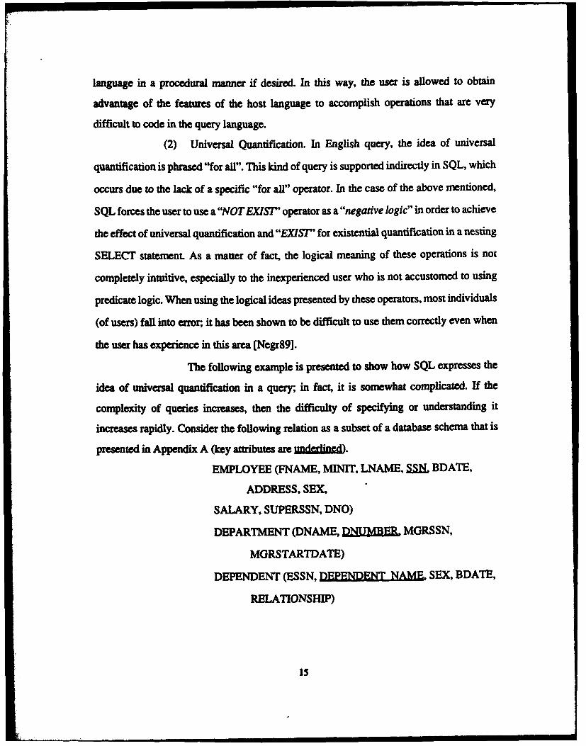
(2) Universal Quantification. In English query, the idea of universal
quantification is phrased "for all". This kind of query is supported indirectly in SQL, which
occurs due to the lack of a specific "for all" operator. In the case of the above mentioned,
SQL forces the user to use a "NOT EXIST' operator as a "negative logic" in order to achieve
the effect of universal quantification and "EXIST" for existential quantification in a nesting
SELECT statement. As a matter of fact, the logical meaning of these operations is not
completely intuitive, especially to the inexperienced user who is not accustomed to using
predicate logic. When using the logical ideas presented by these operators, most individuals
(of users) fall into error, it has been shown to be difficult to use them correctly even when
the user has experience in this area (Negr89].
The following example is presented to show how SQL expresses the
idea of universal quantification in a query; in fact, it is somewhat complicated. If the
complexity of queries increases, then the difficulty of specifying or understanding it
increases rapidly. Consider the following relation as a subset of a database schema that is
presented in Appendix A (key attributes are mdrn•d).
EMPLOYEE (FNAME, MINIT, LNAME, = BDATE,
ADDRESS, SEX,
SALARY, SUPERSSN, DNO)
DEPARTMENT (DNAME, DUMBL MGRSSN,
MGRSTARTDATE)
DEPENDENT (ESSN, DEPENDENT NAME, SEX, BDATE,
RELATIONSHIP)
15

The English query is: "Retrieve the department names in which all of
its employees who have a salary more than $40,000 also have at least one male dependent".
The SQL query is given in Query 2.3.
SELECT DNAME
FROM DEPARTMENT
WHERE NOT EXISTS (SELECT *
FROM EMPLOYEE
WHERE DNUMBER = DNO
AND SALARY < = 40000
AND EXISTS
(SELECT *
FROM DEPENDENT
WHERE SSN = ESSN
AND SEX <> 'M'))
Query 2.3: Ewxmple of SQL Query
The query implements a NOT EXISTS operator in the WHERE-
clause (in the third line) of the query as a negative logic in order to express the universal
quantification. The attribute SALARY is compared as "less than or equal to" instead of
"greater than" in the "outer" nested query and the attribute SEX is also compared as "not
equal" rather than "equal" in the "inner" nested query where the logic of "there exit" is
used for the dependents. Therefore, a direct English translation of the SQL query above is:
"Select the names of departments such that there does not exist any employee whose salary
is less than or equal to $40,000, and there exists at least one dependent that is not "male".
16
The specification required to form the query above is not straight forward at all; the query
formulation involves negative logic that is extremely easy to mix-up, even for the
experienced user. In addition, it is difficult to read and know what is actually being
specified. So, if it is difficult to understand what the query is going to do, it means the
language lacks ease of comprehension and will affect not only query readability but also
the ability of the user to specify the correct query.
(3) Lack of Orthogonality. "Orthogonality in a programming language
means that there is a relatively small set of primitives that can be combined in a relatively
small number of ways to build the control and data structures of the language." (Sebe89]
[Date87]. SQL does not provide the user with a simple, clean, and consistent structure. In
SQL, there are numerous examples of "arbitrary restrictions, exceptions, and special rules."
[Date9Ob]. An example of an unorthogonal construct in SQL is allowing only a single
DISINCT keyword in a SELECT statement at any level of nesting.
(4) Nesting Construct. SQL permits a nesting structure of the form:
SELECT <attribute list>
FROM <relation list>
WHERE attribute IN
(SELECT ......... )
This format allows for a block structure type of construct. The original purpose of
this nesting construct was to allow the specification of certain types of queries without
resorting to the use of relational algebra or relational calculus. According to Codd, the
nesting construct is a part of the "psychological mix-up" in SQL. While all queries that are
specified using the nesting construct should be directly translatable into queries using an
equi-join instead, Codd shows that if allowing for the existence of duplicate rows in tables
(as SQL does), one will come up with a different result when performing the equi-join
17
version of the query than when performing the nested version [Codd9O]. For detailed
descriptions of SQL problems, see [Clar9l] [Wu91].
C. VISUAL-BASED QUERY LANGUAGES
VisMu query languages allow the user to visually specify a query on the screen by
using special graphical editors. Here, visual means not purely textual This kind of language
is also know as a graphical language. We can classify these languages into three categories
of visual-based query languages. The first category includes those which use aform-based
representation, the second is based on the entity-relationship 2 model's (Chen76J
r s ion, and the third includes data flow query languages. In this section we
exanmne QBH as an example of a form-based query language, DFQL as a data flow query
language, and the ER model
L QBE, a Form-based Query Langug
QBE was developed roughly at the same time as SQL during the seventies at
IBM's Laboratory Resoch C (Zloo77]. Today, both languages are available and
supported in the Query Management Facility (QMF)3 offered by IBM. QBE has a user-
friendly interface. While specifying the query, the user does not have to specify a structured
query or tex statement explicitly as in SQL. Instead, the query is formulated by filling/
placing 'Viables" in the proper columns in forms of tables (relations) that are displayed
on the terminal screen. This means that the user does not have to remember the name of
attributes or relatons. Since operations are specified in the tabular from of tables, it can be
said that QBE has a "tvwo-dleional synt,•" [Daw82 [Blma89]. In addition, in QBE
2. Bhuty.iUeouap Model is inooduced by Chen, P. in 1976 5 apkaidal cocueptu desipnmedwddloy for thehadou model3. T7% diaect of QBB suppore in QlF is slihgWy diffemzt from duh proposed by zloof. the orig-Wil ded of QBE [Zloo77], bcm. QlF implemes QBE by fir tum ting it to SQL[DaIM. QMF is a Iein product fora DB2 md act a query lague md report writer
18
there re no rigid syntax rules that should be followed by the user while specifying the
query specification. Instead, the user enters the "variables" as "constant" and "exanpWe"
values in the proper columns of the forms to construct an "exanple" of the data for the
retrieval or update query. Like in SQL, this part also emphasizes data retrieval queries.
QBE is related to the domain relational calculus, and its original specification has been
shown to be relationally complete [Elma89].
a Data Retieval
As mentioned above, in order to specify the query for data retrieval, the
user should enter "example" or "constant" values into the proper columns in the form of
tables (relations). In QBE, the entering of "exanWpe" values, usually preceded by "2-
(underscore) character, means the example value does not have to match specific values of
tuples in the database, so it really represents the "free domain variable". On the other hand,
"constant" values must be matched by corresponding tuple values in the database. If the
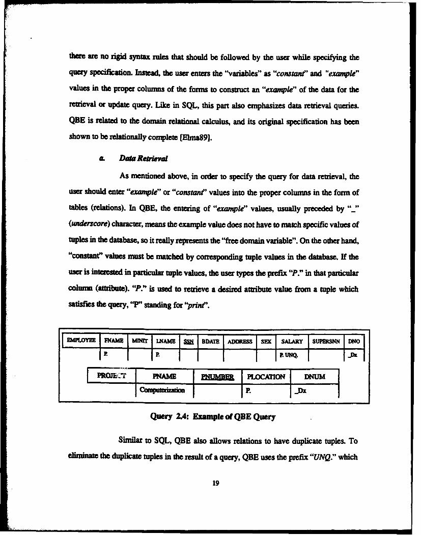
user is interested in particular tuple values, the user types the prefix "P." in that particular
column (attribute). "P." is used to retrieve a desired attribute value from a tuple which
satisfies the query, "P" standing for "prin'".
BebWYEE FNAME~ NMrI LNAME W DDATE ADDRESS SEX SALARY SUPERSNN DNO
RP. P.UNQ.
F~r PNME K=M~iPOCTON MNUMP. x
Query 2.4: Example of QBE Query
Similar to SQL, QBE also allows relations to have duplicate tUples. To
eliminate the duplicate tuples in the result of a query, QBE uses the prefix "UNQ." which
19

means keep only unique tuples in a query result. See the query example in Query 2.4. The
English translation of the query is: "Retrieve the first name, last name, and distinct salary
of employees who works in projects "computerization".
From the example QBE query, it can be determined that:
•"Dx" is an "example" value to join the two tables by using "Dno" as aforeign key
* "Computerization" is an actual "constant" value. In other words, the selecdoncondition using the equality (=) comparison is specified by entering directly a constantvalue under a proper colunm.
S'"P" means to retrieve the attribute value for tuples satisfying the query.
b. Builtin uaniion,., Grouping an" oee Opealn
Like SQL, QBE is also equipped with built-functions, such as CNT. (for
count), SUM., MAX., MIN., and AVG. However, in QBE the functions SUM., CNT., and
AVG. are applied to "diUincg" values. V the user wants these function to apply to all values
desired, it should be entered by using the prefix."ALL" 4. QBE provides a "G." operator as
a grouping aggregate function. It is analogous to the SQL GROUP BY-clause, and the
"condition box" in QBE is used in the same manner as the HAVING-clause in SQL QBE
also uses the same comparison operators as SQL except equality (H). Therefore, the user
explicitly enters the >, >, < , -before typing a constant value. QBE also has a negation
symbol (-,), which is used in a manner similar to the NOT EXISTS in SQL, but the same
effect can also be obtained by using the "-" operator. In addition, QBE also has prefixes
"AO." (for ascending order), and "DO."(for descending order), in order to get an ordered
list of tuples.
4. Ia aQ daer QMF "A,," is umilmd to die kvual qumiAier tE•uMS9.
20

C. Th Proebnl w*k UQE
As mentioned above, QBE is very intuitive, even for novice users. It allows
the relatively inexperiene users to get started in specifying simple queries, even though
they have no prior knowledge of programming languages. Unfortunately, it becomes less
and less useful as the complexity of the queries uicreases and has problems with more
complex queries [Ozso93].
The expression of universal quantification in QBE as originally proposed
by Zloof [Zloo77J did include support for "NOT WE7STS", but it was difficult and always
somewhat troublesome (DwtegOa]. However, today's QBE that has been released as a
commercial product cannot implement universal quantification. In fact, the QBE that we
discuss here (QBE under IBM's QMF) provides no support for universal or existential
quantification of the form of "V" or "3". Thus, queries which involve universal
quantifctdio cannot be specified [Daw ]aJ [Elma89J [Ozso89J. The'efore, it is not
Mkgonay compkft
2. DataFlow Query Lmaga (DFQL)
DFQL is a visual/raphical inteface to relational algebra based on the dataflow
paradigm. It retains all the capabilities of curent query languages and is provided with an
easy to use facility which extends the query language. This extension allows the users to
create new operators from existing primitive or user-defined operators DFQL includes
aggregate functions in addition to the operators of relationally complete query language. It
has the power of expression beyond the benchmark of first order predicate calculus by
providing the user with the capabilties to specify universal and existential quanticaion.
Queries are specified by the user connecting the desired DFQL operators graphically on the
compner screen. The arguments for the operator flow from the bottom or "output node" of
the operator to the top or "input node" of the next operator.
21

a DFQL Op.IIraeI
All DFQL operators have the same basic appearance to enhance the
orthogonality5 of the language. In Figure 2.2. is a sample operator (with no name). It is
made up of three types of components; the input nodes, the body, and the output node.
In DFQL, the functional paradigm is fully supported by the DFQL notation.
The input to each operator, or function, arrives at the input nodes of the operator and the
result leaves from the output node. Thefore, all of the operators of DFQL implement
opetwonal closure. This mean that the inputs to the operators are relations and associated
textual instructions, and the output from each operator is always a relation.
Utnodes
Figre2.2:Operator Cmotu itrdo
In fact, DFQL operators can be grouped into two basic categories: primitive
and user-dflmnd operators. Each priitve has a one-to-one corespodece with an actual
method in the inle-ment1aton language of h interpreter. User-defined opemtors are
creamed from prMve opertors and possibly other user-dfbe operators which have been
previously created. Next, prinitive operators can be brken down into basic, other
prnimives, and display operators.
5. AhoVmdkyaapnV=manalnu r then s ardx iive1y sma tw olpdivs dt-m be scminld in akdy sml s mier aways i bld b e oiui d data wddM s to thie
22
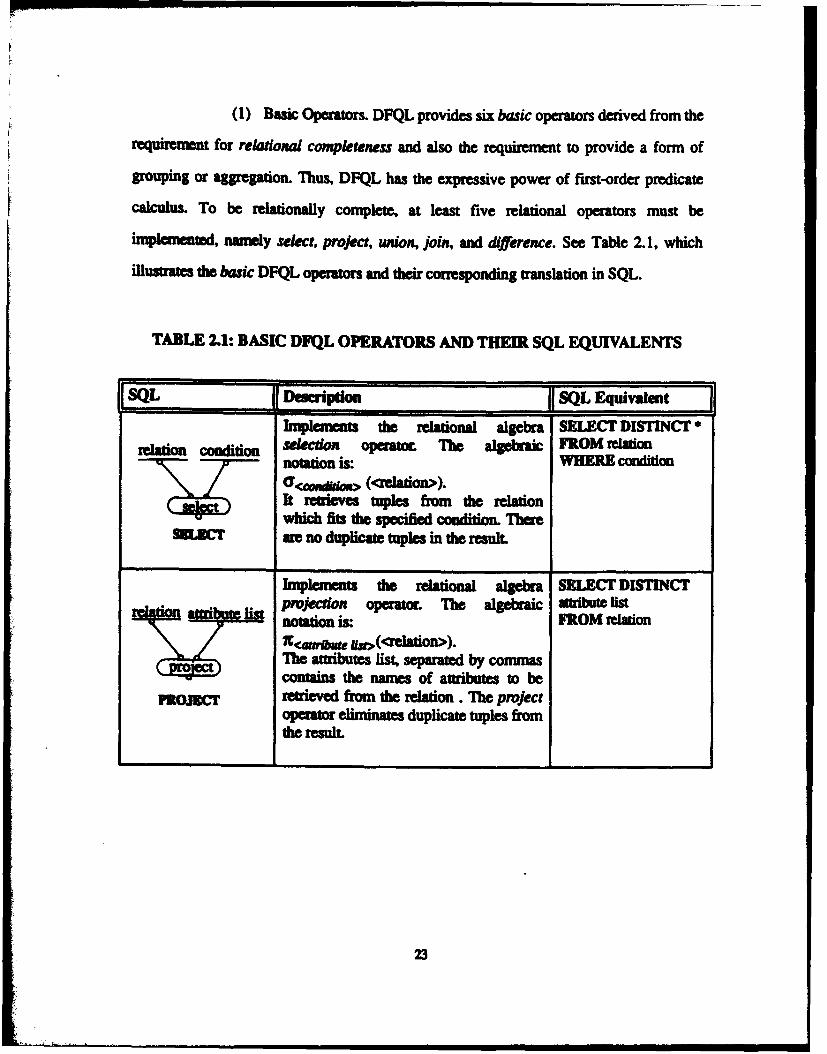
(1) Basic Operators. DFQL provides six basic operators derived from the
requirement for relational completeness and also the requirement to provide a form of
grouping or aggregation. Thus, DFQL has the expressive power of first-order predicate
calculus. To be relationally complete, at least five relational operators must be
implemented, namely select, project, union, join, and diference. See Table 2.1, which
illustrates the basic DFQL operators and their corresponding translation in SQL.
TABLE 2.1: BASIC DFQL OPERATORS AND THEIR SQL EQUIVALENTS
ISQL Desucition SQL Equivalent
Tmplements the relational algebra SELECT DISTINCT, conlio slecdon opeator The algebraic FROM relatio
notation is: WHERE conditionG c0NW04> (<relaion>).
eIt rrieves topics from the relationwhich fits the specified condition. Ther
SELc mare no duplicate toples in the result.
ml n the relational algebra SELECT DISTINCTprojection operator. The algebraic atrbute list
!k is notation is: FROM relationX<wrfft 4>(<re•lmion>).The atibutes list, separate by commascontains the names of attibutes to be
FftIEC retrieved from the relation . The projectoperator -elintes duplicate topics fromthe result.
"23
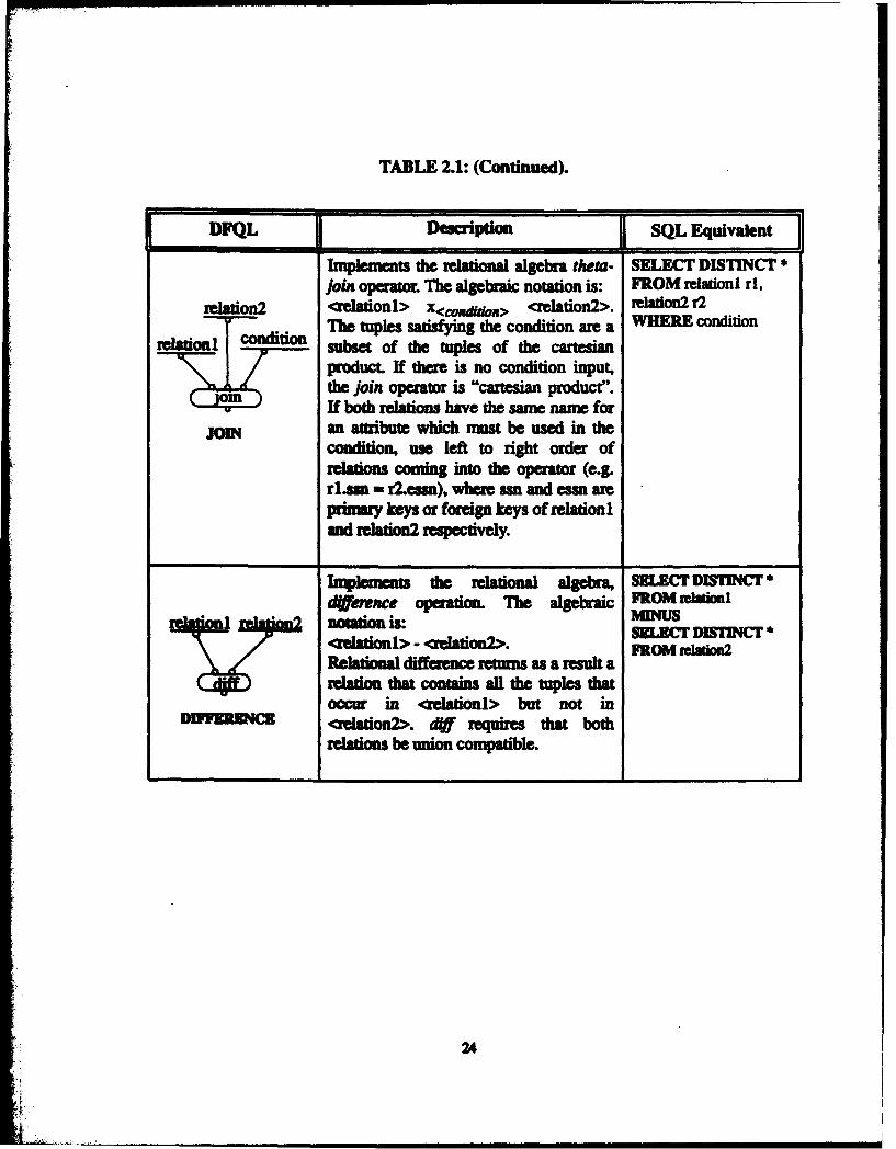
TABLE 2.1: (Continued).
DFQL Description SQL Equivalent
Implemnents the relational algebra theta- SELECT DISTINCTjoin ope= r mtr h algebraic notation is: FROM relationi ri,
relstion2 <relation 1> x~~djn <relation2>. tiatioii2 r2I" r Thetuples satisfying the condition are a WHERE condition
lulUonl codtionl sbset of the tuples of the cartesian
teJoin operator is "cartesian produce'.Nf both relations have the same name for
JOIN an atiuewchmust beusdithcondition, use left to right order ofrelations coming into the operator (e.g.rL~sma = r2.ess), where ssn and esan are
piaykeys or foreign keys of relationiand relation2 respectively.
ImplementsM the relational alerSELF=T DISMICrdpM=e opefatim 7Ue algebraic FRMw~d
I 7 a.i2 notation is:-<relationl> - < jriSELET DIFINC
FROM ielmion2Relational differene returns as a resultarelation that contains all the tuples thatoccur in <relationi> but not in
-~~ <reation2>. dif requires tha bothrelation be union compatible.
24
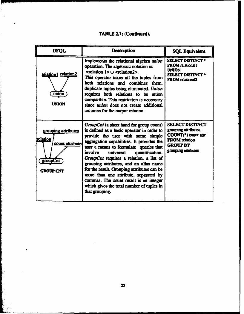
TABLE 2.1: (Continued).
DFQL JjDescription jJ SQL Equivalent
Implements the relational algebra union SELECT DISTINCT *operation. The algebraic notation is: FROM ItflaonallI<r o 1> u < tion2>. UNION
wbfion2 SELECT DISTINCT *This operator takes all the tuples from FtOM 2both relations and combines them,
duplicate tuples being eliminated. Unionunion requirs both relations to be union
"compatible. This restriction is necessaryUNION since union does not create additional
columns for the output relation.
GroupCnt (a short hand for group count) SELECT DISTINCTgoupingattributes is defined as a basic operator in order to stupioo attributes
rlation - proidle th user with some s"pl COUNT( 4 count attircount attrib aggregation capabilities. It provides the FROM relation
user a mns to formujate quetieshat GROUPBYinvolve universal quantification. o mibufsGroupCnt requires a relation, a list ofgrouping attributes, and an alias name
GROUP CNT for the result. Grouping attributes can bemore than one attribute, separated bycommas. The count result is an integerwhich gives the total number of tuples inthat grouping.
25

(2) Other Primitives Opeamtors DFQL provides several other primitive
operators to perform special operations on relations. Most of these additional primitives
perform operations at such a low level that the user would not be able to specify them as a
usser-defined operator. However, all of these additional operators could also be specified as
user-defined operators as well. To illustrate, see Table 2.2. which lists these other primitive
operators and their corresponding translation into SQL.
TABLE 2.2: NON-BASIC DFQL OPERATORS AND THEIR SQL EQUIVALENTS
SQL Description j~SQL Equivalent
Implements relational algebra SELECT DISTINCT *
=W7 on intersection operation The algebraic FROM relationlnotaltion is: EW1iSECT<rltonI <relation2>. SELECT DISTINCT*
intersct Itreturs thetuples which exist in both M Mridnrelatons, as a result out relation.
wrzaswcr Intersect requires both relations to be,union compatible. The i mplementationof intersect is identical to union and diffoperators
Finds the minimumin value of the SELECT DISTINCT
attribtems specifiedj attribute in separated sections gnoupinig attributes,Iaccording to the grouping attributes. It MIN (Upr attr)
anrlate atimr. gesthe grouping atftrites and FROM relationproduces the minimum values of each GROUP butegroup in a column named with the given WouPin M iuealias name as a result Of relation.
GROUP MIN
26

TABLE 2.2: (Continued).
DFQL Description, SQL Equivalent
Sinilar to groupMin except it finds the SELECT DISTINCTes maximum value of the aggregate gOuping attributes,
attributes according to the grouping MAX(aggr. attr.)relation! aa. attribute. FROM relation
GROUP BY group attr.
GROUP MAX
Similar to the previous operator, except SELECT DISTINCT
g attributes it finds the total value of all the aggregate grouping attributes,"relaion agReate attr. attribute's values according to the SUM (aggr. a=.)
grouping attributes. FROM relationGROUP BYgrouping attributes.
GROUP SUM
As previous operators, except it finds the SELECT DISTINCTgrommina attributes average value of the aggregate attributes grouping attributes,
according to the grouping attributes. AVG (aggr attr.)a aFROM relation
GROUP BYgrr'ping attributes.
GROUP AVG
27

TABLE 2.2: (Continued).
DFQL Description SQL Equivalent
It is a simple way of introducing It can be trNIslated into
attributes unversal quantification. It takes a a sequence of SQL
reia c %l cndition relation and splits the tup ies according too the grouping attribute list and then
checks all tuples in individual groupsaccording to the condition specified. If
oupASatisfy, all the tuples satisfy the condition thenan output tuple value is generatedconsisting of the grouping attribute list.
GROUP ALL SATISFY So, it means that this group satisfies thecondition in all their tuples.
This operator is the opposite of It can be translated intogrupin aMibute's groupALSatsfy operator. It gives the a sequence of SQL
retion grouping attributes only if none of the statements-- tiK tuples satisfies the condition.
( eoupNoneSatisfy)
GROUP NONE SATISFY
It is closely related to groupAllSatitj'. It can be taslated into
grouping attriutes The only difference is that groupNSatisfy a sequence of SQLtakes an extra input which allows the StatemeM.
"relation condition user to specify exactly how many of thetuples in the group need to sadsf thegiven condition in order for that group tobe included in the resulting relation. So,the fourth argument (number), must
GROUP N SATISFY consist of one of the operators ( < >, =-,> !-) and a number.
28

(3) Display Operators. The display operators are provided to allow the
user to print the contents of a relation on the computer screen. The most common usage is
to print out the final result of a query. There are two display operators:
"• display. It takes as inputs a relation and a text string to be used as a title. The titlemakes it easy to differentiate between printed results when more than one displayoperator is used in a query.
"* sdisplay. It is used to produce a sorted printout of a relation. Each attribute in the listmay be followed by "ASC" (ascending) or "DESC" (descending).
(4) User-defined Operators. These kinds of operators give the flexibility
to the user to define his/her own style of operator and extend the capability of the language
azcording to his/her desires. With user-defined operators, the user can construct his own
operaturs that look and behave exactly like the primitive operators provided in DFQL The
user can cremae opators for situations that are unique to his query needs. This kind of
flexibility is gained without a loss of the power of orthogonality, since user-defined
operators are constructed by combining the available primitives with previously defined
user operators as well.
(5) DFQL Query Construction. General ideas behind DFQL construction
have been implicitly discussed. Query constructions will be presented in Chapter iM All
DFQL queries exist as data flow programs in which text objects and operators are
connected to each other by lines called data flow paths and all of the information traverse
these paths during execution. DFQL objects, except operations, do not have any input
nodes and can be executed anytime. They pass the relation object, attribute list, or condition
in order to be used by an operator. As soon as all the input nodes have the information, the
operator can be executed and produces a relation at its output node. Since a DFQL query
does not permit iteration and recursion, however, execution of the query can be visualized
29
as flowing from the top the diagram to the bottom. There is no restriction on how operators
are placed on the screen; top-down placement is recommended for readability.
(6) Incremental Queries.This is the most important feature provided by
DFQL. It allows the user to specify or create his/her queries incrementally. In other words,
the user can formulate one portion of the query, and then check the Results (returns back if
needed), and continue to build/create other portions of the query one by one. This capability
gives more flexibility to the user during his/her work, especially when creating a complex
query. It helps the user prevent losing track of what he/she is doing and provides
intermediate results to help in query construction. Specifically, this feature can be div'.-ed
into two sections, namely incremental construction and incremental execution.
"* Incremental Construction. This provides the user with the capability to specify/createthe query part by part, which is ncreasingly helpful as the complexity of the queryincreases
"* Iincreental Execution.This feature is helpful during the debugging of complexqueries. If a complete query does not produce a desired result, it allows the user tocheck level by level in order to find the erroneous part and fix it. Therefore, the usercan see the intermediate result at any level by executing the query incrementally.
(7) Universal Quantification. The problem of expressing universal
quantification in existing query languages has been discussed in previous section. DFQL
provides a unique solution to this problem, by implementing simple counting logic to
achieve the result that fulfill the requirements of universal quantification. The basic idea
employed is that if all tuples in a relation or a group must satisfy some criteria, the number
of tuples that meet the criteria are counted and then compared to the total number of tuples
under consideration. If these two numbers are equal, then the universal quantifier has been
satisfied. In DFQL, the operators that can implement universal quantfication are:
groupAUSadtsfy, groupNoneSadsfy, and groupNSatisfy operators. However, the users can
30

achieve universal quantification as well by building their own quantifications as a user-
defined operator using the primitive operators.
(8) Nesting and Functional Notation. The nesting feature of SQL exists
naturally in DFQL As discussed before, one by one execution of operators to supply input
data to other operator is like block structured execution in SQL from the "inside" to the
"outside" of nesting queries. The lack of specific nesting structures in DFQL improves the
readability and orthogonality of the language. The use of functional notation for all of the
DFQL operators greatly enhances orthogonality. Relational operational closure is
implemented by the functional paradigm. The use of operators that may take more than one
input but produce only one output allows for their easy combination into user-defined
operators as discussed before.
(9) Graphical Structure of DFQL Query. DFQL's visual representation of
the query is a data flow graph consisting of DFQL objects which are connected together
by lines of data flow paths. As such, the graphical structure represents the relational
algebra structure for execution of the query. By using a graphical relational algebra
approach to query formulation, it provides a much more consistent and straight forward
interface to the databases.
3. Entity.Relationship Model Interface
The Entity- Relatonship (ER) model was introduced in [Chen76]. The ER model
has been used extensively as a high-level conceptual data model The main idea behind this
model is to illustrate the concepts of entity types and relationships between entity types in
a graphical way in order to enhance undestanding of the structure desire for a database. An
example of visual representation of the ER model is shown in Figure 2.3.
31

Figure 2.3: ER schema diagram of the COMPANY database [inuaS9]
From the ER diagram we can illustraKe that
• The entty types such as EMPLOYEEE, DEPARTMENT, and PROJECT are
represeted as rectangular boxes.* RationMhip types such as WORKS_FOR, MANAGES, CONTROLS, and
WORKSON are represented as diamond-shape boxes that are attached to thepatiiatn entity types with straight lines.
* Both entity types and relationship types have attributes which are repesnted by theoval/cules where each attribute is attached to its entity type or relationship type bya straight line.
32

" "Name" is an attribute of EMPLOYEE and has composite attributes such as Fname,Minit, and Liname.
"* Location in double ovals represents multivalued attributes, and dotted ovals representderived attributes.
"• Key attributes have their names underlined
"* Double rectangles represent a weak entiy, where the weak entity means an entity typewhich may not have any key attributes, and the double diamond as the identifyingrelationship.
" The partial key of the weak entity type is underlined with dotted line.
"* The participation constraint is specified by a single line for partial participation, withthe cardinality ratio is attached; a double line illustrates total participation. Forexample, the participation of EMPLOYEE in WORKS-FOR is total (every employeemust work for a department), while the participation of EMPLOYEE in MANAGESis partial (not every employee manages a department). MElma89]
The idea of using the ER diagram as a query language is to let the user not worry
about the particularjoin conditions between entity types, however, it tends to force the user
to rely on the specified relationships These relationships are all displayed to the user. This
can be a benefit to a novice user, who does not really understand how the data in the
database fits together, but it seems somewhat fatal, to write queries which depend on
relationships that the user may not fully understand. The ability to use a relationship
without knowing how it is actually set up increases the chance of syntactically correct
queries that will produce the wrong result. The ER model as mentioned above does not
affect our next discussion. It is presented in order to illustrate features of another visual-
based query language that are also available for RDBMS's.
33

HIL THE COMPARISON OF SQI, QBE AND DFQL WITH RESPECT
TO DATA RETRIEVAL CAPABILITIES
First of all, we consider that the notion of a query language as a high level language
means it is intended to be used by a non-programmer or a user without specialized training.
However, as mentioned in two previous chapters, the user faces some difficulties in
specifying correct queries, especially as they relate to universal quantification and nesting
in SQL, and universal quantification in QBE. Then, we attempt to observe how DFQL
overcomes the problems that are encountered by SQL and QBE
This chapter focuses on the comparison of SQL, QBE, and DFQL In order to
accomplish the comparison of these three languages, numerous queries are composed by
category, in which each language is specified and compared. Some of the queries are stand-
alone, but some others specified are logical extensions (or the complexity is increased)
from one query to the next. Such extension types of queries are chosen to analyze the query
language's ease-of-use, flexibility, and consistency in formulating logically related queries
with respect to data retrieval for RDBMS's. Consider the following, brief explanation:
"* Ease-of-use particularly emphasizes how easy the query language is to learn andexpress queries in.
"* Fxibility means more than one way of expressing a single query.
• Consistency means similar thinking in a mental model can be expressed in a similarstructure in the language.
All the representative set of queries presented are matched to the tables of a relational
database instance of the COMPANY schema which are provided in Appendix A. Some of
the queries are related to queries that are presented in [Elma89]. Based on the above, this
chapter is divided into two sections: first the categories of the queries, and second is the
analysis of the strengths and weaknesses of the comparison of all three languages.
34
4• " ' -- . .. ... .. . .
A. CATEGORIES OF QUERY
In order to compare these three languages, numerous queries are composed by
category. The queries are divided into four categories: single-value, set-value, statistical
result, and set-count value. In each category SQL, QBF, and DFQL are specified and
compare&
1. Single-Value
In this category the user (end user) attempts to obtain a proper relation of a
relation (table), based on a single-value expression. As a result of the single value
expression in the queries, the user can expect to obtain a table, a single column, a single
row, or a single scalar value. These correspond to a constant value of table-expression,
column-expression, row-expression and scalar-expression, respectively, in a relation. A
scalar-expression is a special case of a row-expression and a special cae of a column-
expression [Date83]. The null value in this case is also presented as single value (see
Chapter ILA).
In this category, the operators such as "=e,"<" "<=", ">", ">=", and "like", are
generally used in the relation-operation, but we can also perform the standard arithmetic
operators"+" "-", "*" and "r". In addition, if we are concerned with a single scalar value,
a set of special aggregate functions such as COUNT, SUM, AVG, MIN and MAX can also
be applied. In this research these aggregate functions fall under the statistical-result
category. Consider the following queries:
35

AL Qmuy 1: Sbxpl rebfvW
List the salary of every employee.
(1) SQL
SELECT SALARY " SELECT SALARY
FROM EMPLOYEE FROM EMPLOYEE
WHERE TRUE = TRUE
Since in the WHERE-clause we can specify TRUE = TRUE. the
above query can be considered single value. It yields a single column to be a new relation.
If there are multiple employees with the same salary, that salary will be displayed multiple
times as redundant duplicate tuples in the result of the query. If we are concerned with
distinct values, SQL allows us to use the keyword DISTINCT in the SELECT-clause:
SELECT DISTINCT SALARY
FROM EMPLOYEE
The results of these two alternative queries are:
Without keyword DISTINCT With keyword DISTINCT
SALARY SALARY
30000 30000
4000D 40000
2M00 2000
430) 43000
38000 3800O
200 55000
25000
5500O
36

(2) QBE
""LUG M r M •A W ADDRESS s SALARY SUPS
P._Sx
Since we are interested in retrieving the SALARY values, in QBE"P...k" is placed in the column of the SALARY attribute. As discussed in Chapter II, the
prefix "P" is used to indicate that the values of the SALARY column are to be retrieved.
General speaking, QBE allows the user just to specify "P." instead of "P._Sx". In other
words, QBE retrieves the same thing. This seems very simple to specify. However, in some
cases QBE also allows redundant duplicate tuples to exist in the result. In order to avoid
redundant tuples, the prefix "UNQ." is needed as an operator since it keeps only unique
tuples in a query result. Therefore, if we are concerned with distinct values, the "P._Sx"
from the above query can be replaced by "P. UNQ._Sx". The results are the same as for the
SQL query above.
(3) DIFQL
DIPMOYEE Salin_
The attribute list Salary is to be retrieved from the EMPLOYEE
relation. The result of the projection is displayed on the screen by di.play operator. The
37

result is a proper relation which contains only the values from the column of the specified
attribute Salary. Here, the project operator eliminates the redundant duplicate tuples of the
attribute. The result is the same as the SQL query using the DISTINCT operator in "a.(l)"
above.
b. Qury 2: QuaUfied re&b l
List all employees whose salary is more than $50,000.
(1) SQL
SELECT *
FROM EMPLOYEE
WHERE SALARY >50000
The asterisk (*) in the SELECT-clause is shorthand for retrieving all
the attribute values, in order, of uples satisfying the query. The tuple selected must satisfy
the condition "SALARY >50000". Since the query is asking for the list of all employees
who fulfil the condition, the asterisk character should be used in SELECT-clause. The
SELECT-clause retrieves all the employee attributes of tuples from the EMPLOYEE
relation that satisfy the condition specified. There are no redundant tuples in the result.
(2) QBE
MFAWE MWfr F NAM § L S)E ADDESS SEX SAIA SUUSO 1240
1 j >50000
The ">50000" is specified in order to get the tuples that satisfy the
condition "> 50000", where "50000" is as an actual constant value. Placing the "P." below
the relation name means to retrieve all the attribute values of tuples of the relation which
38

match the condition specified. Since the key attribute is included in all tuples returned,
there are no duplicate tuples in the result.
(3) DFQL
EMPLOYEE Sa • 50000
By using the select operator, the query retrieves tuples from the
EMPLOYEE relation which meet the specific condition Salary >50000. There is no
alteration in the structure of the relation, so there are no redundant tuples in the query result
The result of the Query 2 is:
EMLYE NAME Ir Wf LAl SW WDAN ADDRESS SEX SALARY SUPERSSN DNO
Jmu E Barg 89966555 10.Nov-27 450 So.on, 7 TX M 55000 U I
39
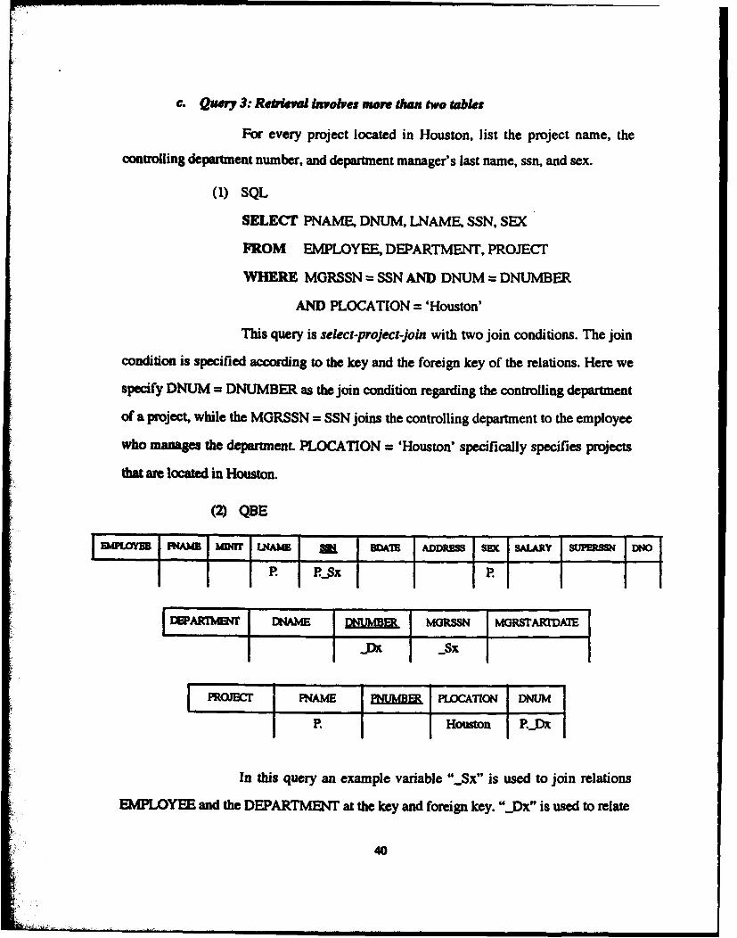
c. Query 3: Rebieval involves more dsaw two tables
For every project located in Houston, list the project name, thecontrolling department number, and department manager's last name, ssn, and sex.
(1) SQL
SELECT PNAME, DNUM, LNAME, SSN, SEX
FROM EMPLOYEE, DEPARTMENT, PROJECT
WHERE MORSSN = SSN AND DNUM = DNUMBER
AND PLOCATION = 'Houston'
This query is select-project-join with two join conditions. The join
condition is specified according to the key and the foreign key of the relations. Here we
specify DNUM = DNUMBER as the join condition regarding the controlling department
of a project, while the MGRSSN = SSN joins the controlling department to the employee
who manages the department. PLOCATION = 'Houston' specifically specifies projects
that are located in Houston.
(2) QBE
EMPLOYU FNAII MM '1 I~m zi W- -U E SLR MSP. P._sx P.
DWRM~ DNAME 3If MORSSN M4RSTARFDA2
PROJECr PNM PNULMBER PLOCA77N I)NVMj
S P. Houston P.J)x
In this query an example variable "_Sx" is used to join relations
EMPLOYEE and the DEPARTMENT at the key and foreign key. "_Dx" is used to relate
40
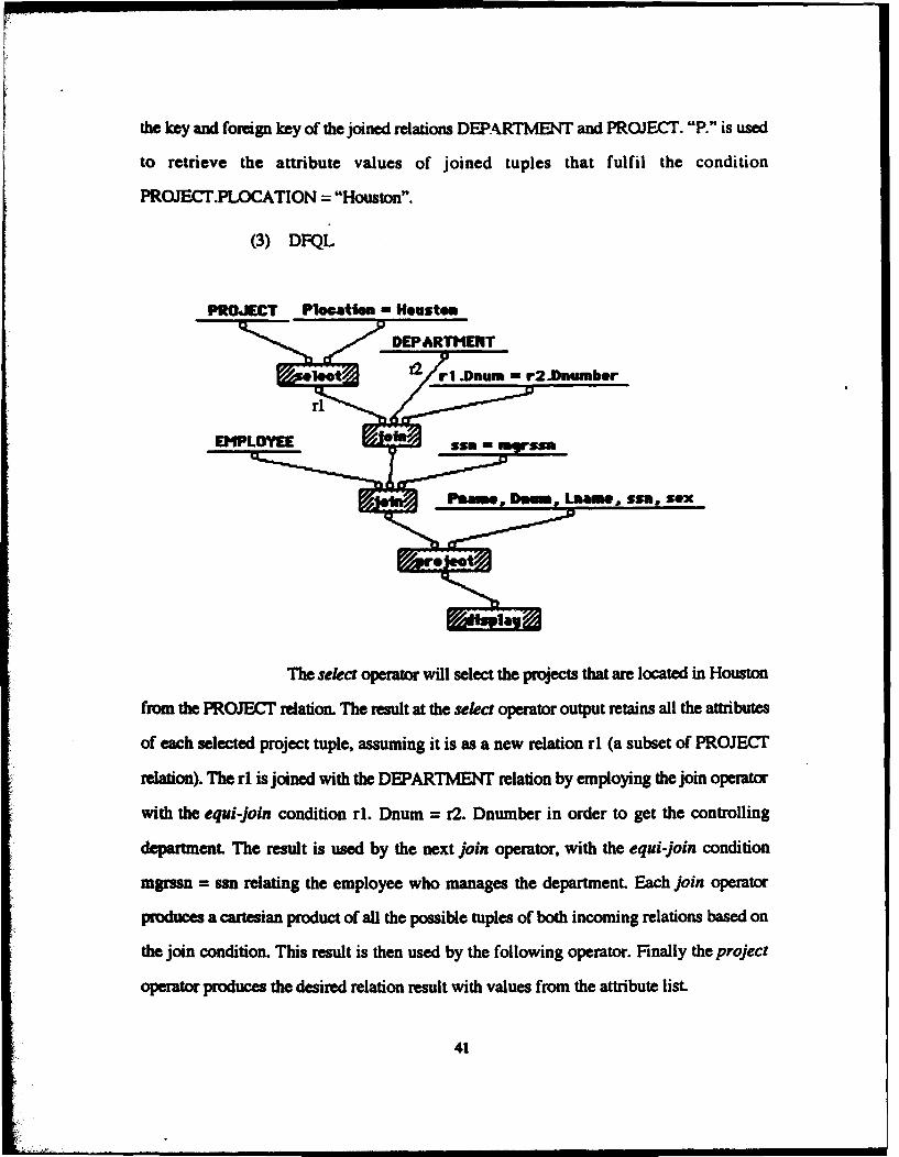
the key and foreign key of the joined relations DEPARTMENT and PROJECT. "P." is used
to retrieve the attribute values of joined tuples that fulfil the condition
PROJECT.PLOCATION = "Houston".
(3) DFQL
PROJECT Plocatlm - Houston
reltin) Te i s oiedwih heDEPARTMENTrlainbemoygthjinprar
wh0 1h rco.Dnu m r2.Doembor
sEMPLO YEE the dprmn E ji
,m~ DanLmsu o
p ue sealcartesianlproduct ofeall rthe possle tue ofebot hat amigrelated in Houston
from the PROJECo rndaiiot The result at the select operator output retains all the attributes
of each selected project tuple, assuming it is as a new relation rl (a subset of PROJECT
relation). The rl, is joined with the DEPARTMENT relation by employing the join operator
with the equi-Join condition rl. Dnumn = r2. Dnumber in order to get the controlling
department. The result is used by the next join operator, with the equi-join condition
mgran = ssn relating the employee who manages the department. Each join operator
produces a cartesian product of all the possible tuples of both incoming relations based on
the join condition. This result is then used by the following operator. Finally the project
operator produces the desired relation result with values from the attribute list.
41
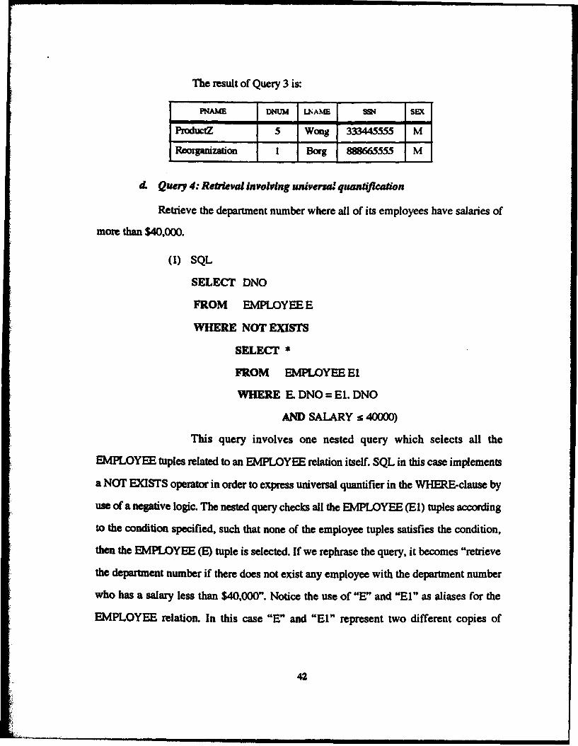
The result of Query 3 is:
PNAME DNUM LUAME S4 SEX
ProductZ 5 Wong 333445555 M
Reorganization 1 Borg 888665555 M
d. Query 4: Rerieval Involving univerml quantification
Retrieve the department number where all of its employees have salaries of
more than $40,000.
(1) SQL
SELECT DNO
FROM EMPLOYEE E
WHERE NOT EXISTS
SELECT *
FROM EMPLOYEE El
WHERE F. DNO = El. DNO
AND SALARY s 40000)
This query involves one nested query which selects all the
EMPLOYEE tuples related to an EMPLOYEE relation itself. SQL in this case implements
a NOT EXISTS operator in order to express universal quantifier in the WHERE-clause by
use of a negative logic. The nested query checks all the EMPLOYEE (El) tuples according
to the condition specified, such that none of the employee tuples satisfies the condition,
then the EMPLOYEE (E) tuple is selected. If we rephrase the query, it becomes "retrieve
the department number if there does not exist any employee with the department number
who has a salary less than $40,000". Notice the use of "E" and "El" as aliases for the
EMPLOYEE relation. In this case "E" and "El" represent two different copies of
42

copies of EMPLOYEE relations. Each DNO will be duplicated if the department has more
than one employee. This can be avoided by using DISTINCT.
(2) QBE. As discussed in Chapter II, QBE lacks the existential and
universal quantification expressions. Therefore this kind of query cannot be specified.
(3) DFQL
Dne Salary o 40000
As discussed in chapter II, DF'QL provides the user some group
aggregate functions that can be used to express the query that contains universal
quantification. One possibility is specified just by employing the groupAllSadsfy. It takes
the EMPLOYEE relation and checks all the tuples in each group of department number
"Dno" that satisfies the condition Salary > 40000.
The result of Query 4 is: none
43

e. Query 5: Retreval Invaolng a negation statement
For each department retrieve the first names and the last names of employees
who have no dependents.
(1) SQL
SELECT DNO FNAME, LNAME
FROM EMPLOYEE
WHERE NOT EXISTS (SELECT *
FROM DEPENDENT
WHER SSN = ESSN)
GROUP BY DNO
The nested query retrieves all DEPENDENT tuples related to the
EMPLOYEE tuple. As in Query 4, this query also uses the NOT EXISTS operator.The
nested query checks all the DEPENDENT tuples to see if the ESSN is the same as the SSN
of the current EMPLOYEE tuple. If none match the nested query returns an empty relation
since there are no dependents associated with the current employee. Therefore, the desired
attributes of the tuple are selected.
(2) QBE
NMO MIM LKM UL DDATEI ADDM S SEX SALARY SUPELSS DNO
P. _Sx G.
DEEDE• EmN DPb)NAM SEX BDAIM RM.ATONSHIP
_S44

By looking at this query, we notice that QBE has a negation symbol
(-). In this case the negation symbol "- " is used in a way similar to the NOT EXIST
function of SQL. It will join tuples of relations EMPLOYEE and DEPENDENT if their
values of "_Sx" do not match each other. However, the query can also be specified by
placing a ",,Sx" in the ESSN column, producing the same result [Elma89].
(3) DFQL
EMILOYIE E
70 Dnol $$1t -ssR
•lkee~a• Fn amewI~m
DFQL provides the groupNoneSatisfy operator which can be used to
specify this kind of query. First, we join both relations EMPLOYEE and DEPARTMENT,
which results in the cartesian product as an input to the groupNoneSatisfy operator. The
groupNoneSatisfy takes the tuples according to the grouping attribute essn and checks to
see if none of the tuples satisfies the condition ssn = essn. If so, the project operator will
project the first name and last name of the employee.
45

In DFQL this query can also be specified by using the diff operator. In
the following query, the inputs to the diff operator are the results of two project operators,
say left and right side. The left side result holds the ssn all of the employee in rl, while the
right side holds the ssn of employees who have dependents in result r2. The di{ operator
checks these two relations rl and r2, and returns any ssn(s) which do not appear in both rl
and r2 as the result, i.e., the ssn of employees who do not have dependents.
EMPLOYEEDEPENDENT
oaoLoam*
The result of Query 5 is:
Fname Lname
Alicia Zelaya
Ramesh Namyan
Joyce English
Abmad Jabbar
Jamesh Borg
46

2. Set-Value
In this category the user (end user) tries to obtain a proper relation from one or
more relation based on the set-value-expression that correspond to a constant-set of query
specifications. In this category, the set operations such as union, difference (minus), and
intersection can also be applied. Consider the following queries:
a Query 6: Refrmval involving existendtal and wiversal quantification
Retrieve the department names, first names, and last names where all of its
employees have salaries of more than $40,000 and have no dependents.
(1) SQL
SELECT DNAME, FNAME, LNAME
FROM DEPARTMENT D, EMPLOYEE El
WHERE D. NUMBER = E. DNO
AND NOT EXISTS (SELECTS
FROM EMPLOYEE E2
WHERE D.DNUMBER = E2. DNO
AND (SALARY :s 40000
OR EXISTS
(SELECT *
FROM DEPENDENT
WHERE SSN = ESSN)))
GROUP BY DNAME
This query is an extension of Query 4 or like a combination of Query
4 and Query 5. SQL specifies this query by employing the EXISTS and NOT EXISTS
operators with two nested queries. The existential quantification is specified by the
EXISTS operator in the nested select statement and universal quantification is expressed
47
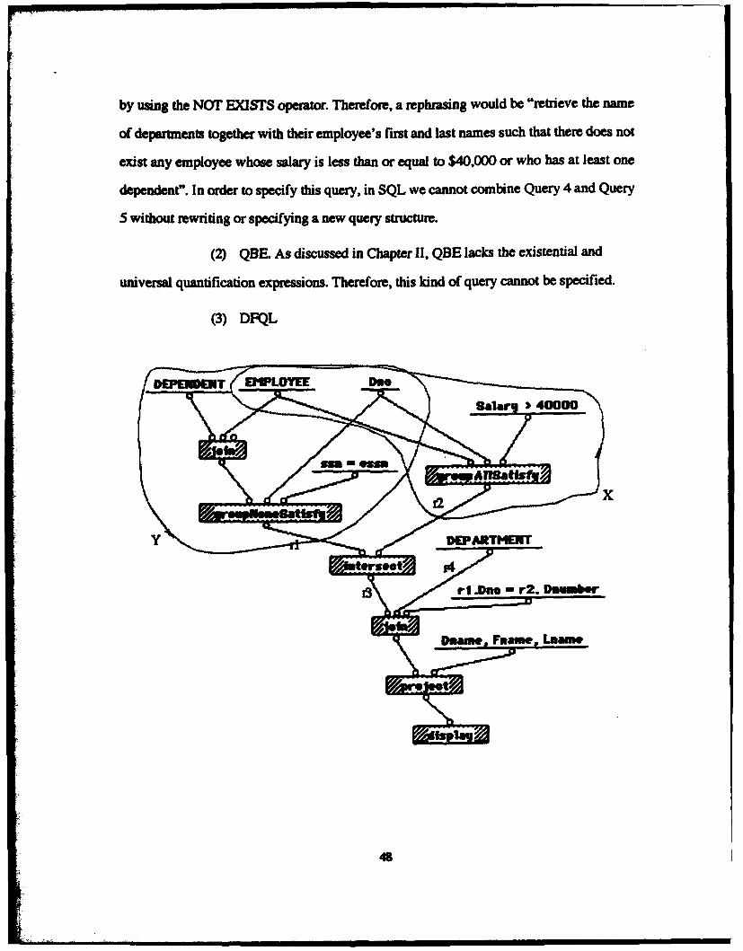
by using the NOT EXISTS operator. Therefore, a rephrasing would be "retrieve the name
of departments together with their employee's riot and last names such that there does not
exist any employee whose salary is less than or equal to $40,000 or who has at least one
dependent". In order to specify this query, in SQL we cannot combine Query 4 and Query
5 without rewriting or specifying a new query structure.
(2) QBE. As discussed in Chapter 1I, QBE lacks the existential and
universal quantification expressions. Therefore, this kind of query cannot be specified.
(3) DFQL
48 40000
vA- W- -f
12[ X

By looking at this query, we recognize this query as a combination of
Query 4 as the "X" part of the query and Y" as the main part of Query 5. The intersect
operator takes two relations which are union compatible (rl and r2) and returns as a result
(r3) the tuples which are in both. Then, by employing the join operator, we join r3 with the
DEPARTMENT relation (r4) based on the aqui-join condition r3. Dnum = r4. Dnumber.
The result is a subset of the cartesian product of r3 and r4 and becomes an input to the
project operator.
The result of Query 6 is:
Dname F-mune Laame
Headquarter James Borg
b. Query 7: RetieMl involving explicit sets
Retrieve the Social Security Numbers of employees who worked on project
numbers 1, 3, and 10 (or maybe more).
(1) SQL
SELECT DISTINCT ESSN
FROM WORKS-ON W1 W2 W3
WHERE WL.ESSN =W2.ESSN AND WI.ESSN = W3.ESSN
AND WI.PNO = 1
AND W2.PNO = 3
AND W3.PNO = 10
This query is retrieving the distinct ESSN attribute of an employee whose
PNO include all values 1, 3, 10 or more. This can be done if the tuples satisfy the condition
which are specified in the WHERE-clause.
49

(2) QBE
WOW-C HWRS
P. UtQ.-XI IUNQ..Y 3U?1k.X,3 10
Condition
I L IIn this case, "P.UNQ._XC", "UNQ.X2", and "UNQ._X3" retrieve
the unique ESSN of an employee whose PNO values include all the constant values 1, 3,
and 10. All of the tuples retrieved must satisfy the condition which is specified in the
condition box.
(3) DFQL
(13S10)
This query shows that a result (r2) of another query makerelaton
which contains the set values (1 3 10) is an input to the groupContainl
50

operato.ThegroaapContain opetator takes the WGRIKS..ON relation Wr) and the second
relaton (42) and groups the tuples according to the grouping attibute essn. It then compares
attribute Poo to see if one essn has all the Pno values contained in r2. If so, the essn is
selected.
The result of Query 7 is: none
c. Q2 ,y 8: Rek nvolWg enxplcitSet
Retrieve the social security numbers of employees who worked on project
number 1, 3, and 10 exactly.
(1) SQL
SELECT DISTINCT ESSN
FROM WORKS-ON Wl W2 W3
WHERE WI.ESSN = W2ESSN AND WI.ESSN = W3.ESSN
AND WI.PNO = I
AND W2.PNO = 3
AND W3.PNO-= 10
AND NOT EXISTS
(SELECT*
FROM WORKS-ON W4
WHERE Wi. ESSN = W4. ESSN
AND W4. PNO o I
OR W4. PNOP3
OR W4. PNO P 10)
I. GroaqContaft opersior is a pat of Groip Set Comparation. GroaqSet Comparoion also pro-vid GmOspgq mad GvopComainBy opmrs. Then opemaor am discussed in clas oes ofDr. C Tlbnes Wu, Coqazier Science Dqluimxnmt Naval Pogadue Scho•, Mtermy, CA.
$i

This query is similar to Query 7. We can use the NOT EXISTS
operator with an included nested query that checks the explicit set Therefore, a rephrasing
would be "retrieve the social security numbers where there are not exists any employees
who worked not on project number 1, 3 and 10". So, it selects exactly the social security
numbers of employees who worked on project number 1, 3, 10.
(2) QBE
SWORON HOURSRUNQ.-XI 1
UNQ._X2 3UNQ._.X3 10
" X4 Px
Condition
XI J~= 2CAND JO JCAND X3-X4I
In QBE, the query is specified according to actual constant values 1.
3 and 10 which satisfy the condition in the condition box. This query keeps a similar
structure to the Query 7. "P.UNQ._XI1, "UNQ.J2, "UNQ._.,3", and "- XC4" are used
to retrieve the tuples which satisfy the condition specified. Notice that the "- .XC4" couple
with the condition "X3 = X4" specifies set equality. An es is selected only if it has PNO
values of 1, 3, and 10 and no other values.
52

(3) DFQL
This query also presents the same structure as query 7. Since the query
is asking to ret'ieve the Social Security Numbers of employees who worked on project
number 1, 3, and 10 exactly, this query uses the groupEqual operator instead of
groupconti operator. It selects the tupies of employees Social Security Numbers only if
the set of no values associated with the essn is exactly equal to (1,3,10).
The result of Query 8 is: noneVORKS53

d. Query 9: Retel involving universal quantifdiaon
Retrieve the first name and last name of each employee who works on all the
projects managed by department number 5.
(1) SQL
SELECT FNAME, LNAME
FROM EMRPOYEE
VCWHERE (SELECT PNO
FROM WORKS-ON
WHERE SSN = ESSN)
CONTAINS
(SELECT PNUMBER
FROM PROJECT
WHERE DNUM = '5)
There are two nested queries. If the set of PNO values from the first
nested query contains all projects that are controlled by department 5, then the employee
tuple is selected. Notice that the CONTAINS comparison operator in this query is similar
in function to the DIVISION operation of the relational algebra [Elma 89].
54

However, for SQL systems which do not have the CONTAINS
comparison operator, the user must specify by using EXIST and NOT EXIST functions, as
in the query below:
SELECT FNAME, LNAME
FROM EMPLOYEE
WHERE NOT EXISTS
(SELECT *
FROM WORKS-ON B
WHERE (B.PNO IN(SELECT PNUMBER
FROM PROJECT
WHERE DNUM = 5))
AND
NOT EXIST (SELECT *
FROM WORKS-ON C
WHERE C. ESSN = SSN
AND C. PNO = B. PNO))
Notice this query involves two level-nested queries. Thus this
formulation is quite a bit more complex than the prior query with the CONTAINS operator.
Consider the first nested query which selects WORKS-ON (B) tuples whose PNO is a
project controlled by department 5 in the IN operator nested query, and there does not exist
a tuple with the same PNO and SSN in WORKS-ON (C) relation which is related to the
EMPLOYEE tuple in the outer query. Since the outer WHERE-clause uses the NOT
EXISTS operator, negative logic is reflected. If the nested query returns the empty tuple,
the EMPLOYEE tuple should be selected. For a detailed description see [Elma89].
55

(2) QBE. As discussed in Chapter II, QBE lacks the existential and
universal quantification expressions. Therefore this kind of query cannot be specified.
(3) DFQL
PROJECT Dgtm - 5
EMPLOYEE VORKS-OR.
that match the condition department number equals 5, then we project the project numbers
from the result into r2. Concurrently, we use the join operator in order to join the
EMIPLOYEE and WORKSON relations according to equality of the keys and foreign
keys esin and ssn into a relation, say r3. By applying the groupContain function operator,
it will compare the tuples of the Pno attributes and splits the group of tuples desired by ssn.
Finally, by using the project operator, we retrieve the desired result. Next, the
groupContain function operator groups r3 by essn. Then groupContain checks to see if an
essn group's set of Pno values contains all the values in r2. If so, all the tuples in the essn
56

group are selected. The result (r4) flows to the project function operator where the desired
attribute values are obtained for display.
The output of Query 9 is:
FNAME LNAMEJohn Smith
.Ramesh &NarvnJoice EnglishFranklin Wong
e. Query 10: Retrieval involving existential and universal quantifiation
List the first name and last name of employees who worked exactly 10 hours
on each of the projects they worked on.
(1) SQLSELECT FNAME, LNAME
FROM EbAPLOYEE E
WHERE NOT EXIST
(SELECT ESSN
FROM WORKS-ON W
WHERE W. ESSN =E,. SSN
AND EXIST
(SELECT
FROM WORKS-ON Wl
WHERE W1. ESSN = E.SSN
AND HOURS < > '10'))
AND
EXISTS (SELECT
FROM WORKS-ON W2
WHERE W2.esn = E-essn)
57
:i I I I l i II I II I
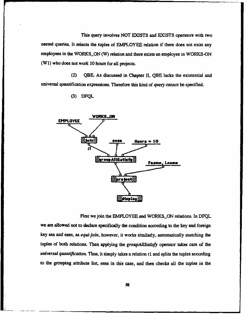
This query involves NOT EXISTS and EXISTS operators with two
nested queries. It selects the tuples of EMPLOYEE relation if there does not exist any
employees in the WORKS-ON (W) relation and there exists an employee in WORKS-ON
(WI) who does not work 10 hours for all projects.
(2) QBE. As discussed in Chapter I1, QBE lacks the existential and
universal quantification expressions. Therefore this kind of query cannot be specified.
(3) DFQL
VORKS..ON
~essa Hemws -: 10
First we join the EMPLOYEE and WORKS-ON relations. In DFQL
we are allowed not to declare specifically the condition according to the key and foreign
key ssn and essn, as equi-join, however, it works similarly, automatically matching the
tuples of both relations. Then applying the groupAlISatisfy operator takes care of the
universal quantification. Thus, it simply takes a relation ri and splits the tuples according
to the grouping attribute list, essn in this case, and then checks all the tuples in the
58

individual group related to the condition Hours = 10. If all the tuples satisfy the condition
specified then the values of that grouping attribute list are passed out. It means that these
groups satisfy the condition by all their tuples. Finally, by using project operator, we
project the desired tuples.
The result of Query 10 is:
FNAME LNAMEII I II
Franklin Woang
Alicia Zelaya
f. Qnery 11: Retrieval involving Set Operation
List of all project numbers and project names for projects that involve an
employee whose last name is 'Smith' as a worker or as a manager of the department that
controls the project.
(1) SQL
SELECT DISTINCT PNAME, PNUMBER
FROM PROJECT
WHERE PNUMBER IN (SELECT PNUMBER
FROM PROJECT, DEPARTMENT, EMPLOYEE
WHERE DNUM = DNUMBER
AND MGRSSN = SSN
AND LNAME= 'Smith')
OR
PNUMBER IN (SELECT PNO
FROM WORKS - ON, EMPLOYEE
WHERE ESSN = SSN AND LNAME = 'Smith')
59

This query uses IN operators and includes nested queries in the
SELECT query. The first nested query selects the PNUMBER of projects that have a
'Smith' as a manager, while the second selects the project numbers of projects that have a
'Smith' as a worker. In this query, the comparison operator BV compares the value
PNUMBER in the outer WHERE-clause and evaluates to true if and only if at least one
value of the sets result from the nested queries matches it. For a detailed description of the
above mentioned and another way to specify this query using the UNION operator, see
[Elma89].
(2) QBE
I MPLOYM MAM t MMNF LNAMd BM DAT AJ)DRES SMC SALMU SUPERSS WNO
S I Smi _Sx I
MAMMMM MOE a~hm MRSSN MGRSAKTDAT
I .... _ . Sx _sI
J _Sx
PUM -f f
In QBE, any number of joins can be specified in a single query
[Elma89]. When we specify a join, we can also specify a result table to display the result
of the query, as in the query above. This is required if the result includes attributes from
60

two or more relations. Sometimes, if there is no result table specified, the system provides
the query result in the columns of the various relation. This tends to be difficult to interpret
and become meaningless in most cases.
(3) DFQL
Since the query involves more than three relations, we make useseveral join operators. Frst we select the last name "Smith" as an employee, then the tuple
result flows to two join operators. One part joins with the WORKSM ON relation on the left
side (we marked as "j 1") and checks to see if the employee is a worker, and on the right
61
•~qrs , ssII I

side (we marked as "j2") joins with the DEPARTMENT relation to check the tuple to see
if the employee is a manager. Since we want to obtain the tuples that relate to Pno and
Pname, we need to join the tuples results of both sides. Then we use the union operator
which takes all the tuples from both sides and combines them (as they are union
compatible). Finally, by employing the project operator, we retrieve the Pno and the Pname
that involve 'Smith' as a worker and as a manager of a department who controls that
project.
The result of Query I Iis: none
3. Statistical Result
In this category the user (end user) attempts to obtain a proper relation from one
or more relations based an a special case of statistical -sultL This category involves
aggregate function operators such as MIN, MAX, AVG, COUNT. Consider the following
queries:
a. Query12: Rekval involving aggregate AVG functon
Retrieve the average hours of working load for project number 3.
(1) SQL
SELECT AVG (HOURS)
FROM WORKS-ON
WHERE PNO = '3'
The average function is used to calculate the average of the values in
the HOURS column from the WORKS _ON relation. The values to be calculated must
satisfy the specified condition PNO = '3' in the WHERE-clause.
62

(2) QBE
WORKS-ON • j. HOURS
3 PAVG. ALL
In QBE, we place "3" as an actual value which represent an equality
condition in the PNO column. And "P.AVG." is used to retrieve the average of the values
that match the condition.
(3) DFQL
- AV 6 (How s): av r " hours.. _
M MG ._(Hou~rs): aierq hours..
The select operator selects the tuples from the WORKS_ON relation
that match the condition specified "Pno = 3". The result is used by next project operator,
which projects the average value of the result according to "AVG (Hours): average
hours...". In this case, an alias name is needed after the colon to indicate clearly what the
result is [Turg93]. The select and project operators are very often used together. So, DFQL
allows the user to define a'new operator by giving a related name selproj as a combine
63
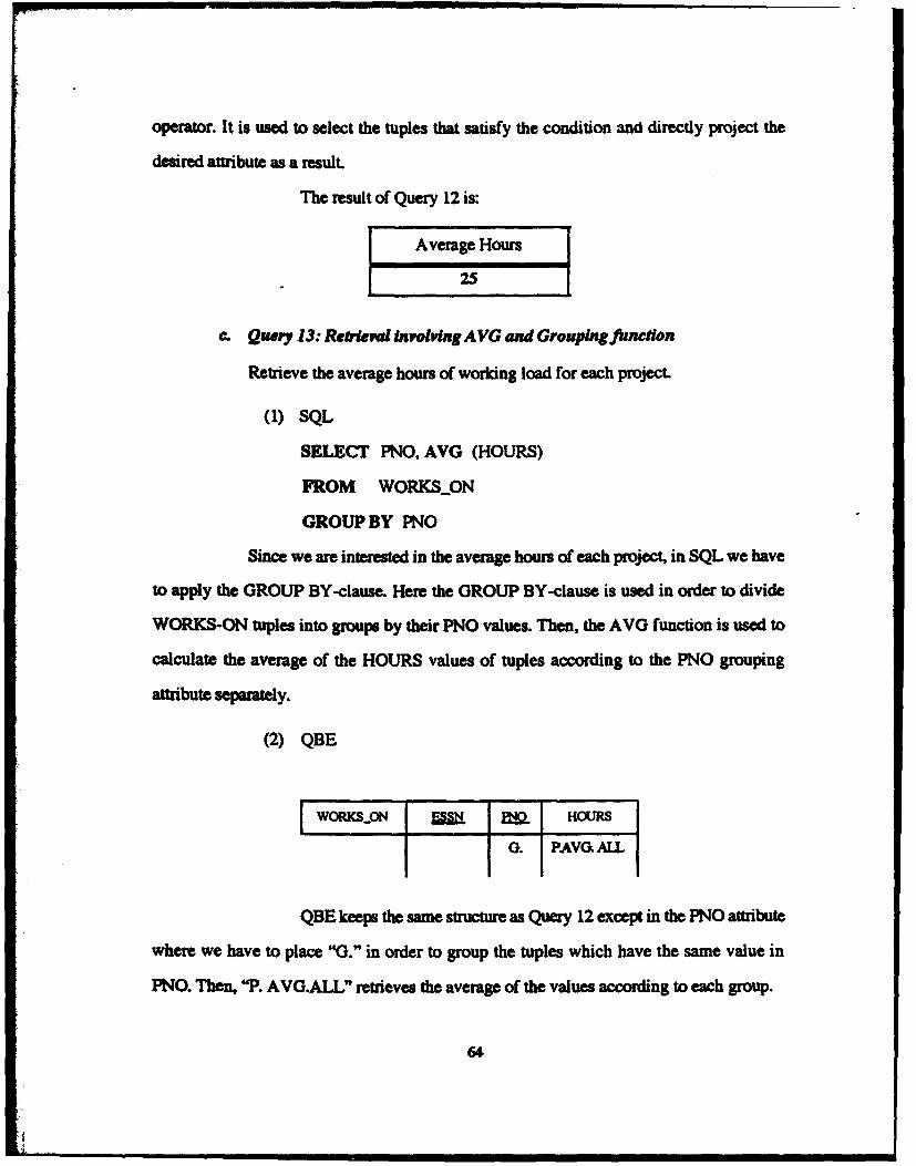
operator. It is used to select the tuples that satisfy the condition and directly project the
desired attribute as a result
The result of Query 12 is:
Average Hours
25
c. Query 13: Rebieml inolving AVG and GroupIng function
Retrieve the average hours of working load for each project.
(1) SQL
SELECT PNO, AVG (HOURS)
FROM WORKS-ON
GROUP BY PNO
Since we are interested in the average hours of each project, in SQL we have
to apply the GROUP BY-clause. Here the GROUP BY-clause is used in order to divide
WORKS-ON tuples into groups by their PNO values. Then, the AVG function is used to
calculate the average of the HOURS values of tuples according to the PNO grouping
attribute separately.
(2) QBE
WORKS..ON fM MQ HOURS
I. PAVG. AML
QBE keeps the same structure as Query 12 except in the PNO attribute
where we have to place "G." in order to group the tuples which have the same value in
PNO. Then, "P. AVG.ALL" retrieves the average of the values according to each group.
64

(3) DFQL
VORKSON PRO lifrs -Awweam bowrs..
DFQL provides several grouping aggregate function operators for
statistical results. One of them is the groupAvg operator. It gets the tuples of WORIKON
relation and splits the tuples according to grouping attribute PNO, then produces the
average of the values of each group of aggregate attribute Hours. The result value is given
an alias name "Average hours".
"Te result of Query 13 is:
Pho Average Hours
1 2625
2 M75
3 25.00
10 27.50
20 12.50
30 27.50
65

d Query 14: Rebieva involving Count, A VG and Groupingfunction
For each project retrieve the project number, the number of employees in the
project, and their average hours.
(1) SQL
SELECT PNO, COUNT (), AVG (HOURS)
FROM WORKS- ON
GROUP BY PNO
In this query, the GROUP BY-clause is needed in order to group
tuples by the project number. Then, the AVG and COUNT (*) operators calculate the
average hours and counted the number of employees respectively for each PNO grouping
from the WORKS-ON relation.
(2) QBE
WORKS-ON Lw M HOURS
RC'.IXALL PG P.AVG.ALL
QBE uses a similar structure to Query 13. Since Query 13 is
expanded by asking the project number and the number of employees involved in each
project, it can be specified by adding "P." beside "G." in the PNO attribute and placing
"P.CNT.ALL" in the ESSN attribute.
66

(3) DFQL
Pmo, ant, AVG (Hours):avorage hours..
This query is an extension of Query 13. The "X" part is exactly the
same as Query 13 and we add the groupCnt function part -Y" that counts the number of
tuples in each Pno group. Here, we need to join the tuples as a result of part "X" and "Y"
which match according to the Pno. Finally the project operator retrieves the desired
attributes from tuples.
The result of Query 14 is:
Pno The number of employees Average Hours
1 2 26.252 3 18M75
3 2 25.0010 3 77.5020 3 12.5030 3 27.50
67
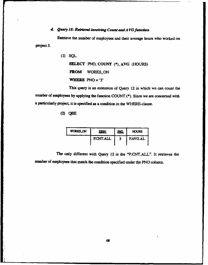
d. Qury IS. Rebridel involving Count andA VOfunction
Retrieve the number of employees and their average hours who worked on
project 3.
(1) SQL
SELECT PNO, COUNT (*), AVG (HOURS)
FROM WORKS-ON
WHERE PNO ='3 6
This query is an extension of Query 12 in which we can count the
number of employees by applying the function COUNT (*). Since we are concerned with
a particularly project, it is specified as a condition in the WHERE-clause.
(2) QBE
WOW-SON 9Mf HOMR
P.CNT.ALL 3 PAVG.AL
The only different with Query 12 is the "P.CNT.ALL". It retrieves the
number of employees that match the condition specified under the PNO column.
68

(3) DFQL
be Avora hours.. X
PRO, "t, AVG (Heurs):average hours....n
In this query, the "X" part is the same as Query 12, and we add the
proupCnt operator "Y" part in order to count the number of employees who participate in
project number 3. Next we need to join the tuples as a result of both sides "X" and "Y".
Then, the project operator is used to retrieve the desired attribute values.
The result of Query 15 is:
Average Hours The number of employees
25 2
69

e. Query 16: Re#riel Involving Max and Grouping function
For each department retrieve the employee's social security number who has
the highest salary.
(1) SQL
SELECT DNO, SSN, MAX (SALARY)
FROM EMPLOYEE
GROUP BY DNO
The employment of the MAX aggregate function is used in order to
obtain the maximum (or highest) value of the SALARY attribute from the EMPLOYEE
relation. We select the tuples with the max salary from each group according to DNO in the
GROUP BY-clause. Based on DNO and highest pay we also retrieve from the tuple the
SSNs attribute value.
(2) QBE
EMPWYE FWAM4 ?dNTf LNAME * BA- ADDRESS SEX SALA"Y SUPE355N O40
P. PM4X.ALL G.
In QBE we just need to specify "G." in the DNO attribute in order to
separate into each group. The "P.MAX. ALL" is specified to get the tuple with highest
salary in the SALARY attribute from all tuples in each group of DNO. And the other "P."
is used to retrieve the SSNs.
70

(3) DFQL
EMPLOYEE Dne Salar.•.
ampay..
I"Tno, max salary]
ioýn De s'mxpay..
The structure which is specified for this query is similar to the
previous queries that involve the groupAvg operator. The only different is we have La use
the groupMax operator. The result of groupMax is the tuple of each Dno group with the
highest pay. Since we are also interested in the ssn of selected employees, we join the
EMPLOYEE relation to the result mentioned above. Then, by using the project operator
we retrieve the attributes desired.
The result of Query 16 is:
Dno SSN Max pay
5 333445555 40000
4 987654321 43000
1 888665555 55000
71
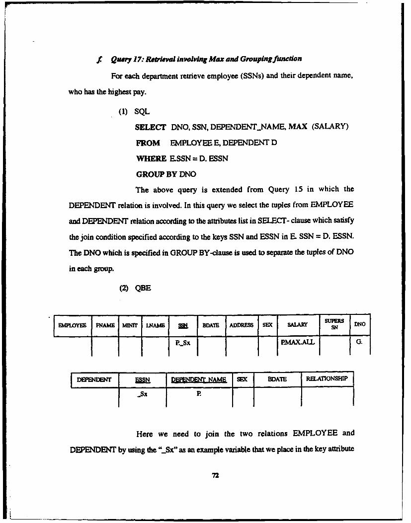
f Quey 17: Retrevl involving Max and Grouping function
For each department retrieve employee (SSNs) and their dependent name,
who has the highest pay.
(1) SQL
SELECT DNO, SSN, DEPENDENT-NAME, MAX (SALARY)
FROM EMPLOYEE E, DEPENDENT D
WHERE E.SSN = D. ESSN
GROUP BY DNO
The above query is extended from Query 15 in which the
DEPENDENT relation is involved. In this query we select the tuples from EMPLOYEE
and DEPENDENT relation according to the attributes list in SELECT- clause which satisfy
the join condition specified according to the keys SSN and ESSN in E. SSN = D. ESSN.
The DNO which is specified in GROUP BY-clause is used to separate the tuples of DNO
in each group.
(2) QBE
F MPIMI FNAMj M LNAME BDATh ADDRESS SE SAUM SUFS DNO
- -I
DEEDEr FMM M AE SEX UDATE RflATONSH[P
_SX P.
Here we need to join the two relations EMPLOYEE and
DEPENDENT by using the "-Sx" as an example variable that we place in the key attribute
72

of SSN and ESSN. The "G." is used to separate the tuples in each group according to the
DNO. Then, "P.MAX. ALL", "P.", and "P._Sx" are used to retrieve the values of the
attributes desired.
(3) DFQL
W tf 016:d dt. top .a.
(Dno, ssn, max, salary]ri DEPENDENT
r"2 r l.ssn - r2. essn
SSU emdent-.naune
Since Query 17 is an extension of Query 16, we see relation r, is a
result of Query 16 which holds the tuples of [dno, ssn, max pay..]. Then we need a join
operator for the purpose of joining with the DEPENDENT relation r2 according to the keys
ssn and essn of both relations. The tuples as a result of the cartesian product that we
obtained from the Jown operator above are used by the project operator in order to retrieve
the values of ssn(s) and the Dependentjname.
73

The result of Query 17 is:
SSN Dependent-name
333445555 Alice
987654321 Abnar
888665555
g. Query 18: Retrieval involving AVG, Max, Sum, and Grouping funcwon
Retrieve the average, maximum and sum of the salaries of each department's
highest paid employee.
(1) SQL
SELECT AVG (SALARY), MAX (SALARY), SUM (SALARY)
FROM EMPLOYEE E
WHERE E.SALARY IN (SELECT DNO, MAX (SALARY)
FROM EMPLOYEE El
GROUP BY DNO)
Again if we increase the complexity of Query 16 to Query 18 as
above, SQL presents a structure which is quite different from the query 16. Here the
GROUP BY concerns DNO in the nested queries in order to separate the tuples and
calculate the highest paid employees. Then, the outer query specifically calculates the
AVG, MAX, and SUM values of the highest paid of all groups in the department.
74

(2) QBE
BM~Y !FNAWJ MMINIT LNME W BDAIE ADDRESS SEX SALARY UM M DNO
PAMAX.ALL G.
Resu 1 Dept. top payP MAXAUAVG.ALLSUM.AL
In QBE, this type of query can be specified into two steps, where first
we attempt to retrieve the highest paid according to each group of the DNO. Then we
retrieve the attribute values of selected tuples by placing the "P." under the Result column
and "MAX.ALLAVG.ALL.SUM.ALL" under the Dept. top pay column.
(3) DFQL
OR ii of dept. top paY aon pa .
'75
'~a (ma II I I I I

Again, in this query the results of Query 16 can be used as a source or
as an input to the other group operators. In the case of this query groupStati operators are
used to perform the calculation of avg (max salary), sum (max salary), and max (max
salary). Here, each of these operators produces the values we are concerned with.
The result of Query 18 is:
Avg (max pay) Sum (max pay) Max (max pay)
46000 138000 55000
& Query 19. Rehievl involving Count and Groupingfincion
For each department retrieve the department name and the total number of
employees who are paid more than $40,000.
(1) SQL
SELECT DNO, DNAME, COUNT (*)
FROM EMPLOYEE., DEPARTMENT
WHERE DNUMBER = DNO AND SALARY > 40000
GROUP BY DNO
Like the previous queries, the GROUP BY-clause is used to separate
the tuples into groups by DNO attribute value. Then, the values of the attributes listed in
SELECT-clause are selected from EMPLOYEE and DEPARTMENT relation in the
FROM-clause which satisfy the conditions specified in the WHERE-clause.
I. Group" opematr is digmssed in now of Dr. C. Thoa Wu, Compuut Science Deparment
76

(2) QBE
DEARflv4B'1 LtAME QftUflE. MORSSN MORSTARDMAM
EMFWYEE PHAMS MD1T LNAM UL BDATE AMS SEE SALARY SUtBI DNO
l i ii I >40000 PO.CNT.ALL._Dx
In this query the "P.G.CNT.ALL-Dx" is specified in order to retrieve
("P.") the tuples based on the grouping "G." of DNO attribute, and CNT. ALL is used to
count DNO in each group to represent the number of employees. All of these can be
performed if the tuples match ý -join condition specified by "..Dx" according to the key
and foreign key DNUMBER and DNO.
77

(3) DFQL
EsPLOYEE se t 40000
DlqEPARTMENTthe num2 rl ber ofeploee
D" ome, oult
First we select the tuples of the EMPLOYEE relation that fulill the
condition Salary > 40000. Then we join the result of the se:ct operator with theDEPARTMENT relation by equality of the key and foreign key Dnumber and Dno. Then,
the result is used by the gromp~ht operaw which splits the tuples according to Dno groups.
RnalBy, by using the project opertowr, we retrieve the values of the dname and dno, and also
the number of employees.
The result of Query 19 is:
Dname Dno The number of Employees
Administiutionr 1
A74

4L S*-Comt Value
In this category the user (end user) is interested in obtaining a proper relation from
one or more relations based on a special cas of set-count testing. Consider the following
queries:
a. Query 20: Retriwal involving eziuttial quantification
Retrieve the first name and the last name of managers who have at least one
female as a dependent
(1) SQL
SELECT FNAME, LNAME
FROM EMPLOYEE
WHERE EXISTS(SELECT
FROM DEPENDENT
WHERE SSN = ESSN
AND SEX ='F')
AND EXISTS (SELECT *
FROM DEPARTMENT
WHERE SSN =MGRSSN)
One way to specify this query as shown above involves two nested
queries. The first nested query selects all DEPENDENT tuples, and the second selects the
DEPARTMENT tuples managed by the EMPLOYEE Therefore, if there exists at least one
tuple dependent with SEX equal to female in the first nested query, and at least one tuple
of the employee who managed the department; then the EMPLOYEE tuple is selected
according to the FNAME and LNAME of the employees.
"79

(2) QBE. As discussed in Chapter II, QBE lacks the existential and
universal quantification expression. Therefore this kind of query cannot be specified.
(3) DFQL
DEmP RTIH MI
F j EaPLO rEE joi t E Y dTr o u
W DEPENrDEN----'•'-"r I.ssn =- r2.ess
SSox- F ,-*cLn ,
First we join the EMPLOYEE and DEPARTM4ENT relation by using
the equi-join based on their key and foreign key, in this case ssn = migrssn. Then, the tuples
as a result of the eqsd-join, say as rl flows to the next join operator. At this point r I contains
the tuples of employees who manage a department joined with DEPENDENT relation. say
r2, according to the key and foreign key join condition rl.ssn = r2. essn. Then, by applying
selproj operator, we select the tuples desired which satisfy the condition specified "Sex =
F" and directly project or retrieve the values of Fname and Lname of the manager.
The result of Query 20 is:
Fname LnameFranklin Wong

b. Quay 21: Rekw~ l involing Cout and Grouping funtion
Retrieve the total number of employees with salaries more than $40,000 who
worked in each department, but only for those departments where more than four
employees work.
(1) SQL
SELECT DNAME, COUNT (*)
FROM DEPARTMENT, EMPLOYEE
WHEIRE DNUMBER = DNO AND SALARY > 40000
AND DNO IN (SELECT DNO
FROM EMPFLYEE
GROUP BY DNO
HAVING COUNT (*) > 4)
GROUP BY DNAME
While reading Query 21, it can lead to misunderstanding the point in
specifying the SQL query. It may lead us to specify the query as follows:
FROM DEPARTMENT, EMPLOYEE
WHERE DNUMBER = DNO AND SALARY > 40000
GROUP BY DNAME
HAVING COUNT (*) > 4
This is an incorrect query since it will retrieve only departments that
have more than five employees who each earn more than $40,000. For a more detailed
description of the above queries see [Elma89].
Query 21 is expanded from Query 19 in the previous Section "3. h.",
but they are very different in structure. Query 21 is specified by using the nested query.
While specifying this kind of query we must be careful, especially when we have to apply
81

two different conditions like the query above; where "SALARY > 40000" is applied to the
COUNT function in the SELECT-clause and the other in the HAVING-clause. And for the
GROUP-BY function, Elmasri comments "Some SQL implementations may not allow a
GROUP BY-clause without a function in the SELECT-clause. Hence, the nested query in
this example (Query 21 (1) SQL) cannot be permitted in such SQL implementations".
(2) QBE
DWARTMF DNAME M E MGRSSN MGRSTAIJrDATE
P. Dx I
EMPLOYES PAME 1Dm LNAMM UL BDATE ADDRESS SEX SALARY SUPESN DNO
>4OO00 P.G.CNT.ALL._Dx
ConditionSCM4TALL._Dxk> 4
Here, QBE really keeps a structure similar to Query 19. Here we need
to specify in the condition box "CNT.ALL.._Dx > 4" in order to retrieve the total number
of employees if it is more than four members in each department according to the value of
DNO.
82
-k ' " mr • • mm

(3) DFQL
Sine tisexandd romQulwy 19, we4nue0l0o0uey0~
Th result of uera21is:non
Aft

e. Query 22: Retrieval involving Count and Grouping function
For each project on which there are three or more employees working,
retrieve the project number, project name, and number of employees who work on that
project.
(1) SQL
SELECT PNUMBER, PNAME, COUNT (*)
FROM PROJECT, WORKSON
WHERE PNUMBER = PNO
GROUP BY PNUMBER, PNAME
HAVING COUNT (*) > 3
This query involves two relations PROJECT and WORKS-ON. Here,
the GROUP BY-clause is used in order to separate the project in each group and selection
of tuples is used to satisfy the join condition in WHERE-clause. The HAVING-clause in
this case uses whole groups of projects, and specifically specifies the number of employees
which satisfies the groups themselves.
84

(2) QBE
PROJECT PNAME R PLOCATION DNUM
P J11~
WORKSON E E HOURS
PG.CNrALLJIX
Condition
[LJ a
Here, P.G.CNT.ALL.Px" is specified in order to retrieve the tuples
of the grouping attribute of PNO which satisfied the join condition related to the key of
PNUMBER and PNO. But, it must satisfy the condition box "CNT. ALL_Px > 3". Here
the use of the condition box is similar to the HAVING-clause in SQL
85

(3) DFQL
PROJECT VORKS.ON Paumber PRO
Sc~~nt ,3
Pname, Pnumber, ct
We join the two relations PROJECT and WORKS-ON according to
the join condition Pnumber = Pno. The tuples of the cartesian product is flowed to
groupCnt operator, and it splits Pno into each group. Then, it selects the tuples that fulfil
the condition specified "cnt a 3"as counting the number of employees. Through the project
operator we retrieve the tuples needed according to the attribute list.
The result of Query 22 is:
Pname Pnumber The number of employees
ProductY 2 3
Computerization 10 3
Reorganization 20 3
Newbenefit 30 3
86

d Queay 23: Retkva involving Countwfnion
Retrieve project name, where there are three or more employees.
(1) SQL
SELECT PNAME
FROM PROJECT
WHERE (SELECT COUNT (*)
FROM WORKS-ON
WHERE PNUMBER = PNO) at 3
By modifying Query 22 just a little bit, we get Query 23. One way to
specify the SQL query is shown above involving a nested query. The nested query counts
the tuples (representing the number of employees) involved in the project in the
WORKS-ON relation. If it is greater than or equal to three, the PROJECT tuple is then
selected. In some implementations of SQL the above query may not be permitted [Eima89].
(2) QBE
PROJ:c- PIAME Fa1X PLOCATION DNUM
P Y
WORKSON HOURS
I AT.Au._JPxa a3
In this query "CNT. ALL._Px a 3" counts the tuples concerning the
number of employees. If it is greater than or equal to three then the tuples of Pname areretrieved by "P." according to key as specified by an example value ".Px".
87

(3) DFQL
PROJECT VORKS-ON Pnumber - Pne
Sout 3- 3
&lo Pname
isplayl
In order to get the counting result, DFQL in this case applies the
groupCnt operator in all kind of queries that relate to set count query. That's why Query 22
and Query 23 are specified with exactly the same structure, just slightly different in the
attribute list of the tuples desired.
The result of Query 23 is:
Pname The number of employees
ProductY 3
Computerization 3
Reorganization 3__
Newbenefit 3
By looking at the results of Query 22 and 23, we notice that the tuples
results of PNAME and the total number of employees retrieved are absolutely equal. In
short, we can say that both Query 22 and 23 are really the same in the structure.
88

e. Query 24: Retieval involving universal quantification
Retrieve project name, where there are three or more employees, and all of
them has a work load of 20 hours.
(1) SQL
SELECT PNAME
FROM PROJECT P, WORKS-ON W
WHERE P.PNUMBER = W.PNO
AND PNO IN (SELECT PNO
FROM WORKS-ON
WHERE HOURS = 20
GROUP BY PNO
HAVING COUNT (M) z3)
Query 24 above is an extension of Query 23. In the SQL query above,
the GROUP BY-clause and HAVING-clause are particularly related to PNO in the nested
query. If each group of PNO tuples satisfies the condition "HOURS = 20", and also if in
each PNO there are three or more employees as a worker, then the PROJECT tuple will be
selected. However, it must satisfy the join condition specified in the WHERE-clause.
(2) QBE. As discussed in Chapter II, QBE lacks the existential and
universal quantification expressions. Therefore this kind of query cannot be specified.
89

(3) DFQL
PROJECT VORKSON Pn.r P,, o e
eat ),,
*1--'Pao Hours -- 20
Consider the DFQL query above. Part "X" is Query 23, and it can be
directly used as a relation to be an input to the groupAiLSalisfy operator. It takes the tuples
and splits the tuples according to the PNO as a grouping attribute, and the tuples in each
group must satisfy the condition specified "Hours =20". Then, we retrieve the tuple result
of the attribute desired by using the project operator.
The result of Query 24 is: none
90

f Query 25: Retkral Involving universal quantification
Retrieve the department names which offer two or more projects where there
are three or mom employees who worked on it, and all of them has a work load of 20 hours.
(1) SQL
SELECT DNAME
FROM DEPARTMENT D, WORKS-ON W, PROJECT P
WHERE D.DNUMBER = P.DNUM
AND P.PNUMBER = W.PNO
AND PNO IN (SELECT PNO
FROM WORKS-ON
WHERE HOURS = 20
GROUP BY PNO
HAVING COUNT () a:3)
GROUP BY DNUM
HAVING COUNT (*)a 2
Query 25 is expanded from Query 24, and the complexity of the query
has increased. This query involves three relations and nested query. A GROUP BY-clause
and HAVING-clause are used specifically for the nested query, and another GROUP BY-
clause and HAVING-clause are used for the whole groups. Even though this query is just
slightly different from previous Query 24, we have to rewrite while specifying this query.
91

(2) QBE. As discussed in Chapter 11, QBE lacks the existential and
universal quantification expressions. Therefore this kind of query cannot be specified.
(3) DFQL
PROJECT WORKS..DN
mt 3= X
I"t PoeHos - 20
------ ------ -- DEP RT M E N
Notice that the "X" part is Query 24. The tuple result is directly used
as a relation to beoirhed• with the DEPARTMENT relation accordling to the key and foreign
key Dnumber and Dnum. The result of the cartesian pnvduct which is produced by the join
92I

operator flows to the groupCnt operator which groups according to the grouping attribute
of Dnum. Then, by employing the selproj operator we can count specifically the tuples
which satisfy the condition specified, and directly project the values desired of the attribute
list.
The result of Query 25 is: none
B. ANALYSIS
In the previous section, we observed how SQL, QBE, and DFQL specify all of the
query examples which are composed in categories. Queries range from simple ones to
queries which involve existential or universal quantifications, and complex nested queries
in SQL. Some of the queries are stand-alone, but some others specified are logical
extensions in complexity from one query to the next. By examining these queries the
relative strengths and weaknesses related to ease-of-use, especially in expressing universal
quantification, specifying the complex nested queries, and flexibility and consistency in
formulating the queries with respect to data retrieval for RDBMS's are investigated.
1. Ease-of-use
Ease-of-use of query languages is part of the human factor aspect. In this research
we emphasize the learning and writing of the query, as well as attempting to retrieve the
output result. However, we have to keep in mind that query languages are high level
languages that are also intended to be used by non programmers. Related to Ease-of-use,
some researchers described that:
" The SQL language has been designed and intended to be easily learned and used byinexperienced user without specialized computer training [Reis75].
"* The result of various psychological studies of language (QBE) show that it requiresless than three hours of instruction for non programmers to acquire the skill to makefairly complicated queries [Zloo77]. People will write queries in QBE between two orthree times faster than in SQL [Reis8lJ.
93

* DFQL is proposed and implemented to mitigate problems that are encountered by thecurrent query languages, SQL in particular. It requires about half an hour in a databaseclass at NPS to acquire the concept and make more correct queries than SQL [Clar9l].
According to our research through the previous Section "A." of this chapter, the
above comments and results are absolutely valid for QBE and DFQL but not for SQL
Consider the representative sets of queries that we have in each category or from one
category to the other categories. Here ease-of-use of each language can be pointed out
clearly, where "once we learn a general construct from a sample query, if the way of
thinking can be applied in a new query" we can say that there is certain degree of ease-of-
use. For example, when we learn the technique to drive a car for 500 yards, then we could
most likely can drive for another 1000 yards. Now, let' s take a look at some of the queries
that we have.
a. Qucrks involving existmntial or unversal quantfiaion
In the following discussions we covers several queries that are composed in
single-value, set-value, and set-count value categories. Consider the queries below:
* Query 4: Retrieve the department number where all of its employees have salaries ofmore than $40,000.
* Query 5: For each department retrieve the first name and the last name of employeeswho have no dependents.
* Query 6: Retrieve the first name, last name and department names where all of itsemployees have salaries of more than $40,000 and have no dependents.
By looking at these three queries we realize that Query 6 is virtually the
combination of Query 4 and 5. Now let's consider how do SQL, QBE, and DFQL construct
all of these queries.
(1) SQL See the construct of the structure of Query 4 and Query 5, where
both queries contain NOT EXISTS operators that interpret the queries in a negative logic
approach. Generally, these kind of query structures are not easy to understand, especially
94
Query 4. Assume, we understand the construct of both queries, however we cannot apply
this similar thinking to specify the structure of Query 6. In this case, we do have to think
very carefully since we have to specify a new query that may be very different in the
structure. Therefore, these types of queries are difficult to specify even for the experienced
users.
(2) QBE. QBE lacks universal quantification expressions. Therefore we
cannot express these types of queries.
(3) DFQL By learning the construct of Query 4 and Query 5, we can use
the similar thinking of Query 4 and Query 5 in order to form a new Query 6. Once we know
the construct of Query 4 and Query 5 we can use them in the other new query easily. Noticein Query 6 that the "X" part retrieves the tuples of employees who have salaries of morethan $40,000, as Query 4, and that the "Y" part retrieves employees who do not havedependents. We can logically combine these two constructs by using the intersect operator
that combines union compatible tuples so that we have the tuples of all employees who
have salaries of more than $40,000 and have no dependents. Since we are interested in the
department name also, we can easily join the tuples result above as new relation (63) withthe DEPARTMENT relation (r4) which match according to the key and foreign key of both
relations, r3. Dno = r4. Dnumber. Finally, by employing the project operator we retrieve
from the tuples the first name, last name, and department names of those employees.
By investigating the above queries, once we learn how to specify
Query 4 and Query 5, we can generalize them in a straight forward manner to specify Query
6. We can say that this language is easy to learn (and thus easy to use). Consider the
following queries that are similar to the above discussions:
See Query 9, 10, which are difficult to specify in SQL, cannot be specified in QBE(see QBE description in Chapter II.C. 1.c.), but are very easy in DFQL since we canapply the construct concept of Query 4.
* Query 20 also shows that in SQL it is not easy to learn or understand the structure, andin QBE it cannot be expressed. (See QBE description in Chapter II.C. 1.c.). But inDFQL the data flows from one part to another are easy to follow and one can
95

undestad what's going on.
b. Queries involving neted queries
In this section, we analyze queries which involve the BN operator in the nested
query. In addition, we also examine several queries which contain the universal quantifier
in the nested queries. Consider the following queries in the set-count value category:
Query 21: Retrieve the total number of employees with salaries more than $40,000who worked in each department, but only for those departments where more than fouremployees work.
However, before going into any detail in Query 21, see first Query 19 in the
set-value category. By examining these two queries we realize that Query 19 is expanded
to Query 21.
* Query 19:. For each department retrieve the department name and the total number ofemployees who are paid more than $40,000.
Similar to the above description "l.a." we attempt to learn the construct from
one sample query and extend it to create another new query. Consider how SQL., QBE and
DFQL construct both queries:
(1) SQL When we learn Query 19 and understand the construct, we arestill not confident of how to specify the structure for Query 21 (or an incorrect query can
be specified, see SQL query below Query 21). In other words, in SQL we cannot use the
construct of a sample query to build a new query in a straight forward manner.
(2) QBE In QBE we realize that the same thinking of the construct in
Query 19 can also be used to specify Query 21. QBE in this case presents a simple and very
intuitive extension.
(3) DFQL When we learn the construct of Query 19, it is easy to
understand Query 21. Here, the construct of Query 19 can be used as a part of Query 21.
To build Query 21 we know that we need two parts; first the employees with salaries more
96

than $40,000 and second, tuples of those department with more than four employees. See
Query 21 of DFQL for details.
We also look at several queries which are similar to the abovediscussion. These types of queries are composed in the set-value, statistical-result, and set-
count categories. Consider the queries below:
"* Query 7 is extended to Query 8.
"* Query 16 is extended to Query 18.
"* Query 22 is modified to Query 23.
• Query 23 is extended to Query 23.
* Query 24 is extended to Query 25.
In addition to discussion in "l.a" and "I.b" above, see Query I in the single-
value category. If we are interested in the di"tinct value, in SQL we have to use the keyword
"DISTINCT" in the SELECT-clause, and in QBE the prefix "UNQ.". On the contrary,
DFQL implements the primitive operators which have a similar capabilities to the
relational algebra operators, so the duplicate tuples in the query result are eliminated. In this
case, we consider that DFQL is easy to use, since we do not need to worry when and where
we have to eliminate the duplicate tuples. For detailed problems concerning the duplicate
tuples see [Codd9OJ.
Next we examine the query that involves select-project-join with two-join
conditions. See Query 3. In SQL it is not easy to comprehend what is going on in the query.
QBE in this case presents a simple construct in which it is easy to follow the joining
between relations and we know what's going on. Furthermore, in DFQL we can easily
follow how the data flows from one part to the other part. It is understandable.
97
2. Fleldbility
The flexibility which is offered by each language, is considered very useful in
specifying queries. Therefore, we feel free to choose the techniques which are most
comfortable and confident in order to specify the correct query. However, by having
numerous ways of specifying the single query, it may introduce confusion about which
technique to use to specify particular types of queries [Elma89].
a. SQL
SQL supports join conditions that can be used to specify many queries or use
nested queries with or without the IN operator in it. See Query 9. Instead of using the
CONTAINS operator we can use NOT EXISTS and the IN operator with a nested query.
Also Query 11 that uses IN and OR operators can be specified using the UNION operator.
Sometimes, queries in which are involved NOT EXISTS may be specified using the IN
operator with nested query or vice versa. Query 8 is an example. It can be specified without
the IN operator. Generally speaking, there are numerous ways to specify the same query in
SQL (Elma89]. However, in some cases we have no confidence that our query writing is
well specified or correct.
b. QOB
QBE provides less syntax than SQL and DF;QL, therefore it does not have the
flexibility like SQL does. However, the tuples result that are existed in several relations can
be formed in one result relation. This flexibility makes the query result more meaningful.
See Queries 11 and 18
96

c. DFQL
DFQL provides primitive operators as described in Chapter II and also we
have been demonstrated in Section "A" of this chapter. DFQL in this case, offers the
flexibility to the user to use the combination or stand alone of the primitive operators with
respect to the query concern. In queries which involved universal quantifier, like Query 4,
instead of using the groupAIUSatisfy operator we can apply the select and groupCnt
operators. In Query 5, instead of using the groupNoneSatisfy operator we can also apply the
diff operator in the main part of the query. In addition, DFQL allows the user to define their
own user-defined operator such as the selproj operator of Queries 9, 10, 22, and 25.
Furthermore, the output of one query can be used as an input or as a part of another new
query. In fact, once we know the concept of each operator, we can use it in query
construction easily. In DF-Q.., we feel more confident that our query is correct, since we
can trace or check the flow to the result part by part.
3. Consistency
As described before, our investigation here is focused on the structure of queries
specified in each language. If a mental model that we have for one sample query can be
built or continued to another new query, where the new query keeps the same mental model
of structure with the prior query, we can say that the language is consistent in structure.
Consider the queries in the single-value, set-value, statistical-result, and set-count value
categories:
"* Query 6 is extended or combined from Query 4 and 5. All of these queries involveuniversal quantification.
"• Query 7 and 8 involve explicit set.
"* Queries 12, 13, 14, 15 relate to AVG function.
"* Queries 16, 17, and 18 relate to MAX function.
99

* Query 19 is extended to Query 21.
* Query 22 is modified to Query 23, then Query 23 is extended to Query 24. FinallyQuery 24 is extended to Query 25.
By using the various query examples above, we can examine the structure of
SQL, QBF, and DFQL For detail, see and compare the structure of each query. Consider
the following brief explanation:
a. SQL
SQL is not consistent in structure. If we attempt to extend the queries
(complexity increases) as the queries above, so far we cannot apply our mental model of
one construct of query structure to the next new query. In fact, we have to rewrite a new
query from the beginning, which will often be very different in structure (inCo- ,istent) with
the prior queries. Therefore, inconsistency in specifying queries in SQL, exists and is
confusing to the user.
b.QNE
QBE is very intuitive. In specifying the queries which are presented above
QBE is very consistent in structure. The mental models that are formed in one query can be
continued to other new queries easily, except for queries that involve universal
quantification. Since QBE lacks existential and universal quantification expressions, this
kind of query cannot be expressed.
c. DPQL
DFQL exhibits consistency in structure. If the queries are extended, we can
use the output of a query result, whether a portion or the whole of a previous query, to be
a part of other new queries. This flexibility is not exhibited in SQL, nor in QBE. Even
though the queries are extended (complex ty increases), DFQL remains consistent in its
structure of query.
100

4. Relative Strengths and Weaknesses
In this section we present the relative strengths and weakness of these three
languages. The following result is presented by referring to our previous discussion plus
some general descriptions of each language. The relative strengths and weaknesses of SQL,
QBE, and DFQL are summarized in Table 3.1.
101

I Al.
A Ai
4~ 18
80E-10
*1102

S!1!.
i• 11Iiii:Iii

V -j
,i,..jig
'II
N..
tow, C
104
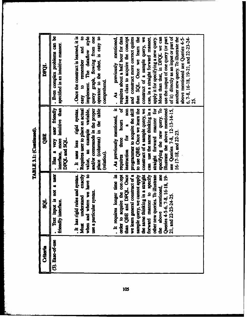
IA!.~ r* ~84
Si R~ Ss ;.
I! AKSS 0Ioi j6 &'~I~
- a 320Sie.04
P asI- 0 1~q
%]g
9 1 0 .Q
eiia
105

:1 . Nj 00
4Q cai~r*
Cjgw
I %w
0 O0r

91.-6 .cy . 9 a 'S.
VA S 0a 9
'IC
.s1
010

slI I *11r~icr
E.1 .9
0 0 108

a71oi c00
0.
8~ V
'00 C:
Js
109

*� E �O� 0
*d �0
�!��iII1o.J� .�2 :;�
Ua'.
� *0 �
ii 0
A- a'U
ij�, e..- bO
- Wau, a
C
Uit Ia�c#2� i�i �,
*� -a'
a �
� �
I
110

IV. HUMAN FACTORS EXPERIMENT
A. HUMAN FACTORS ANALYSIS OF QUERY LANGUAGES
There are several query languages commercially available, and there is a need to
examine a variety of different query languages in order to measure the notion of "ease-of-
use" of query languages. The most common approach in capturing what is the query
writing, in which subjects are given questions in English and asked to write the
correspotlding query language statement (Reis8 1].
B. EXPERIMENTAL COMPARISON OF SQL, QBE, AND DFQL
In this section, we review a very simple human factors experiment for comparing
SQL, QBE, and DFQL A general assessment of the experiment is provided. Since we
know that QBE cannot express universal quantification (see Chapter H. C. 1. c), the tasks
are divided into two parts:
" First part consists of five queries which can be specified in SQL and DFQL. In thisgroup universal quantification is required.
" Second part consists three queries which can be specified by all three languagesSQL, QBE, and DFQL Universal quantification is not included.
This experiment is not intended to be a rigorous comparison of SQL, QBE, and DFQL
1. Amuement of the Experiment
In this experiment 15 subjects were given five tasks of query in English on the
relational database schema of Appendix A. The subjects coded or specified each of the
query task. Three query tasks were applied to all three query languages, and two query tasks
just applied to SQL and DFQL. Each response was then graded as either correct or
Incorrect.
!' I11

a Subjects
The experiment was conducted on 15 students enrolled in "Advance
Database" and "Database Seminar" courses at the Naval Postgraduate School (NPS) in
Monterey, California. The students at NPS are primarily U.S. military officers; foreign
military officers and Department of Defense civilian employees are also represented. The
composition of the student are recorded based on their academic backgrounds, which are
broken down based on their bachelor degree which is classified as "technical" or "non-
technical". In addition, subjects are also characterized by their programming experience.
For analysis purposes, subjects with programming experience more than 1 year are
classified as "experienced".
b. Teaching Method
All the subjects have already taken the introductory database system course
for one quarter, so all of them have a background in relational algebra, relational calculus,
SQL and QBE. A 30 minute presentation of DFQL concept was given at the beginning of
the experiment A handout describing the DFQL operators was given to the subjects.
a Test Queri
The five test queries were based on the relational database schema in
Appendix A. They are:
" Query Ql: 'List the name and location of the projects whose member (at least one)earns more than $40,000." The first query (QI) involved only selection, projection,and joining to achieve the correct answer.
" Query Q2: "For each project, list the number of employees working on that project.""The second query required grouping and counting. Here the comprehension issomewhat more complex than Q1.
"* Query Q3: "Retieve the total number of employees who worked more than or equalto 20 hours in each project, with more than two employees working." The third query,in addition to gouping and counting operadons, also required special condition thatneeded another grouping and counting; in SQL, it is specified by HAVING-clause.
112
"• Query Q4: "Retrieve the name of each employee who works on all projects that arelocated in Houston." The fourth query required the DIVISION operation of relationalalgebra, in SQL it could be specified wether using CONTAINS comparison or NOTEXITS operators. In DFQL, it can be specified using groupContain operator.However, since QBE lacks universal quantifier, this type of query can not beexpressed.
" The question QS: "List the first name and last name of all employees who have onlyfemale dependents." The fifth query required the use of the universal quantifier andwas subjectively viewed more difficult than the first three queries, but almost the samewith query Q4. Here, SQL applied NOT EXISTS operator in the WHERE-clause, andin DFQL specified by the groupAllSatirfy operator. Similar to the fourth query, itcannot be expressed by QBE.
By providing five queries which were of increasing complexity, it was
intended to see if DFQL perform better than SQL and QBE in more difficult queries.
Subjects were given one week to complete the experiment.
A Evaluation MethWd
The tests were collected and hand-graded by the researcher. The criterion
evaluated by this experiment was graded as either correct or incorrect queries. Correct
included responses that were either completely correct or contained a minor !anguage or
minor operand error. The following taxonomy of minor language error and minor operand
eror were given by Welty and Stemple [WeltSl]. A minor language error is a basically
correct solution with a small error that would be found by a reasonably good translator. A
minor operand error is a solution with a minor error in its data specification, such as a
misspelled column name. However, a transposition of column names (or simple use of the
wrong colmnn name) was classified as an incorrect answer because there is no way for the
grader, or computer to determine the subject's intent.
113
2. Experiment Results
In this section we present a general discussion of the results derived from the data
taken. The primary measurements of this experiment were made based on the entire sample
population. The primary metric used was the number of questions answered correctly. This
was calculated for each individual question and also for each language as a whole, the result
are summarized in Table 4.1. In addition we also provided the results based on subject
bac ounds (technical/non-technical and programming experience). However, since the
percentage differences between SQL, QBE, and DFQL for all queries were nearly similar
and the number of subjects in individual classification was small (due to small overall
population size), the detailed statistical analysis was performed only on the total sample,
see Table 4.2 and Table 4.3.
From Table 4.1., for the easiest query (QI), subjects wrote a greater percentage of
correct answers in SQL than in QBE C7%) or in DFQL (20%). But, in Q2 there was a
difference of 53% for conrect answer in DFQL compared to SQL and 40% compared to
QBE. In Q3, them was only 7% more correct answers in DFQL compared to SQL and 0%
conmpared to QBE. For Q4 the difference was 7% between DFQL and SQL. In Q5 there was
a difference of 33% for correct answers in of DFQL compared to SQL In the above
analysis, we always subtract the SQL and QBE percentages of correct answers from DFQL4
a difference of 20% means that DFQL produced 20% moe correct answers than SQL or
QBE.
Table 4. summarizes the percentage of correct queries for SQL, QBE, and
DFQL for Q1, Q2, and Q3 broken down by techical/non-technical as well as experienced/
non-experienced. We see that the subjects with a non-technical background got a slightly
greater percentage of queries correct in all three languages than those with a technical
backround. The diffevence was 3% more correct for SQL, 2% for QBE, and 9% for DFQL
114

In classification by experience, there was no difference in percentage of queries correct for
SQL, while the less experienced subjects got 8% more correct for QBE queries, and the
more experienced got 3% more correct for DFQL.
Table 4.3. summarizes the percentage of correct queries for SQL and DFQL for
Q1 through Q5 broken down by technical/non-technical as well as experienced/non-
experienced. We see that the non-technical got a slightly higher percentage correct for both
(3% for SQL and 1% for DFQL). The experienced subjects got 7% more correct than the
less experienced for SQL and 8% more correct for DFQL.
TABLE 4.1: EXPERIMENT RESULT
% OfCorrectThas
SQL QBE DFQL
Q1 87 go 67
Q2 40 53 93
Q3 6 13 13Q4 33 Not1Cowmpua 40
Q5 0 Not Coipa*k 33
Overalof the 33 49 50first" part which
Q1 tbrOng Q5.
Overal of the 44 49 58nacm part
whichcontains
Ql, Q2, and Q3.1. Not Com_ -, sie QE lks of univerd quandfi.2. Overall Atm pao is caculmed for all the tme anguagesSQL. QDE and DIQL3. Ov=m econd put is cbaued jus for SQL and DFQL
115

TABLE 4.2: PERCENT CORRECT OF SUBJECT CLASSIFICATION FORQ1, QZ, AND Q3
Subject Number % Of correct
Chmiaa tiou of Subjects SQL QBE DFQL
Technical 7 43 48 53
Non-Technical 8 46 50 62
Experincel> Yr. 12 44 47 59
Expeiience! <1 Yr. 3 44 55 56
Total Sample 15 44 49 58
TABLE 4.3: PERCENT CORRECT OF SUBJECT CLASSIFICATION FORQ1 THROUGH Q5
Subject Number % Of CormctCiauflctio of Subjects SQL DFQL
Technical 7 31 51
Non-Technical 8 34 52Thpueee1yr. 12 32 45
E Rmesce 1 Yr.. 3 39 53
Total Sample 15 33 50
116
3. Experiment Coautem
Generally speaking, since this human factors experiment was conducted on only
15 subjects, the result is not a rigorous statistical comparison of SQL, QBE, and DFQL
However, we still can make the following observations:
'L Qary (Qi)
SQL is better than QBE and DFQL for a simple query which involves only
selection, projection, and joining, that is a query in the single-value category. Once the user
learns and knows the concept of this type of query, it is easy for the user to build another
query in a single-valmue category as long as the query requires only project, select, and join
operations. See a representative query (Query 3) in Chapter HIL A.l.c., which requires a
simple selection and projection without a need of nesting. As long as nesting is not
require, SQL seems to provide a simple and logical query construct.
b. Qwey (QP)
DFQL is better than SQL and QBE for queries requiring grouping and
counting operations. This kind of query composes statistical result. In DFQL, the idea of
grouping and counting is easy to understand since it requires just one operator (groupCnt).
See Query 14 as one similar to Q2. In SQL, some of the subjects misunderstood how the
COUNT operator works, and they specified GROUP BY followed by an attribute name but
did not specified this attribute in the SELECT-clause. In QBE, some of the subjects mixed-
up the CNT and CNT.ALL operators.
&. Qmuer (Q3)
In this query all three languages had an approximately equal percentage of
correct anwer. Query (Q3) requires grouping, counting functions and special condition.
In SQL the special condition is known as HAVING COUNT (*), and in QBE it is normally
117

specified using condition box. In DFQL, it is formulated by using groupCnt followed by
select operators. A representative of this kind of query is illustrated by Query 21 which is
composed in set-count value, Chapter M. A. 4. b. Since Q3 increases in complexity
compared to Q2, logically Q3 is more difficult. If subjects did not have a good
understanding of the concept of this type of query, normally they come up with incorrect
query. For instance in SQL, this query requires nesting, with GROUP BY and HAVING
COUNT () operators in the nested part and another GROUP BY is needed for the whole
query. Therefore, we can say this type of query was more difficult to formulate in SQL
compared to QBE and DFQL.
A Quay (Q4)
Query (Q4) exhibited no significant difference in percentage of correct
answers between SQL and DPQL. This type of query requires the DIVISION operation of
relational algebr, which is similar to Query 9 (set-value category, see Chapter MLA. 2. d.).
For SQL, this quey is easy if the subject understands the relational division and the SQL
impl suppom the CONTAINS operation. In cases where the CONTAINS
operation is not available, it would be much more difficult because either.
* User has to tansate relational division into equivalent relational operations, and thenwrite the SQL coresponding to the translated relational operations, or
* User has to re-think in SQL using operations such as the NOT EXISTS operat. Inthis case, user has to change his/her mental model to negative logic while formulatingthe quay.
Query (QS) involves existential or universal quantification. In SQL the NOT
EXISTS and EXISTS operators with two nested queries are required to specify the query.
This kind of quey is similar to Query 10 which is composed in set-value, Chapter IIL A.
2. e. Since the NOT EXISTS is used the user must think in the negative logic, which is more
Ila

difficult to formulate even for the experienced users. Not one of the subjects formulated a
corect answer in SQL for this query (QS). However, in DFQL, universal quantification can
be formulated just by using the groupAlSatidfy operator. Therefore, for queries which
involve universal quantification, DFQL offers a more understandable approach than SQL.
By examining these five tasks, for a simple query which requires selection
and projection without nesting, SQL seems a simple and logical construct. However, for
queries which require grouping, counting and universal quantification, DFQL seems better
in specifying the query than QBE and SQL
119

V. CONCLUSIONS
There are some known problems with a widely used query language such as SQL and
QBE. Some of the problems are the lack of expressing universal quantification, specifying
complex nested queries, and flexibility and consistency in specifying queries with respect
to data retrieval. To alleviate these problems, a new query language called "DFQL" was
proposed. We conducted a comparison of three languages: SQL, QBE, and DFQL
Numerous queries were grouped into four categories, single-value, set-value,
statidcal result, and set-count value; specified in SQL, QBE, and DFQL, and compared in
each category. In the queries comparison, queries ranged from the simple ones to queries
which are involved existential or universal quantification and complex nested queries
Some of the queries are stad-alone, while some others specified are logical extensions of
owe query to the next, with the complexity increasing (refer to Query 1 through 25 in
C maptrI). Thwe rqiesentative sets of queries were chosen in order to investigate the
relative shuagths and weaknesses of each language related to ease-of-use issues, especially
in apressing universal q fic , nested queries, and flexibility and consistency in
specifying the queries with respect to data retrieval for RDBMS's.
In this research, based on the above queries mentioned, and the analysis which are
smnmrized in Table 3.1., we conclude that DFQL eliminates the problems which are
e PoCnerd by SQL and QBE mentioned above. The relative strengths of DFQL comes
nainly from its strict adherence to relational algebra and dataflow-based visuality. Strict
adherence to relaional algebra allowed users not to worry about exceptions as was the case
with SQL Dataflow-based visuality required users only to master a very simple and
intitive dataflow paradigm to write queries. A simple paradigm of dataflow suffic even
for a very complex query, because the complexity of the query is handled by high-level,
uwer-dqlied operaions, not by extending the language construct as is the case with the
120

other two languages. Although the number of subjects in our experiment is too small to
conclude affirmatively that DFQL is better than the other two, the result of the experiment
showed that DFQL's ease of query writing resulted in a greater percentage of correct
queries, especially queries which involved count, grouping functions and universal
quantification (complex queries), than in either SQL or QBE.
121

LIST OF REFERENCES
(ANSI86J American National Standards Institute (ANSI), The Database LanguageSQL, Document ANSI X3. 135-1986 (1986).
[Astr76] Astrahan, M. M., et aL, System R: Relational Approach to DatabaseManagement, ACM Transactions on Database Systems, vol. 1, no.2, pp. 97-137, June 1976.
(Cham74] Clamberlin, D. D., and Boyce, R.F., SEQUEL: A Structure English Querylanguage, Proceedings of the ACM-SIGFIDET Workshop, Ann Arbor,Michigan, May 74.
[Chen76] Chem P. P., The Entity-Relationship Model -- Toward a Unified of Data,ACM transactions on Database System, vol.1, March 1976.
[Clar9l] Clark, G., and Wu, C. T., Dataftow Query Language for RelationalDatabase, Department of Computer Science Naval Postgraduate School,Monterey CA.
[Codd70] Codd, E. R, A Relational Model of Data Large Shared Data Bank,Comnication of the ACM, voL 13, no.6, pp. 377-397, June 1970.
[Codd7l] Codd, . F., Relational Completness of Data Base Sublanguages, CourantComputer Science Sypuosium 6, Data base Systems, pp. 65-98, May 1971.
[Codd88a] Codd, E. F., Fatal Flaws in SQL: Part I, Datamation, voL 34, pp. 45-48, 15Augu s198.
[Codd88b] Codd, E. F, Fatl~ Flaws in SQL: Part II, Datamation, voL 34, pp. 71-74, 1September 1988.
[Codd90] C ldd, E. F., The Relational Model for Database Management: Version 2,Addison-Wesley, 1990.
[Date82] Date, C. L., An Inoduction to Database Systems, Third Edition Addition-Wesley, 1982.
(Datc84] Date, C. L, A Critique of The SIQL Database Language, ACM SimnodRecord vol. 14, no. 3 pp. 8-54, November 1984.
[Date87] Date, C. ., Where SQL Falls Short, Datamation, vol 33, pp. 83-86, 1 May1987.
122

(Date90a) Date, C. J., Relational Database Writings 1 985-1 989, Addison-Wesley,1990.
[Date9ObJ Date, C. 3., An Introduction to Database Systems, Fifth Ecditon, Addition-Wesley, 1990.
[E~ma89l Ehmasri, R., and Navathe, S. B., Fundamental of Database Systems,Benjamn/VCummings, 1989.
[Fra88J Frank, L, Database Theory and Practice, Addison-Wesley, 1988.
(Hans92J Hansen, G. W., and Hansen, J. W., Database Management and Design,Prenitice Hfall, 1992.
(Negr89] Negri, M., Pelagatti, 0., and Sbattela, L., Short Notes: Semantics andProblem of Universal Qatfcion in SQL, The computer Journal, vol. 32,pp.90,91, 1989.
[Ozso89] Ozssoyoglu, 0., Matos, V., and Ozsoyoglu, Z. M., Query ProcessingTechniques in the Summary-Table-by-Eamiple Database Query Language,ACMI Transactions on Database Systems, vol. 14, no. 4, pp. 526-573,December 1989.
(0uso93J Ozsoyoglu6 G., and Wang, IL, Example-Based Graphical Database QueryLangguaes, Computer, vol. 26, no. 5, May 1993.
[Rci75] RdIsam~ P., Boyce, KR.F, and Chamberlin, D. D., Human factors evaluationof two data base query Languages-square and sequel, AFIPS Proceedings,vol. 44, pp. 447-452, May 19-22, 19175.
[Reis8l] Resime, P., Human Factors Studies ofDatabase Query Languages: A Sureand Assessmnent, Computing Surveys, vol. 13, pp. 13-3 1, March 18
(Sebe89J Sebesta, R. W., Concept of Programming Languages, Benjamitn Cumming,1989.
[Sclm78] cniemn B., Imp roving the Human Factors Aspect of DatabaseInteractions, ACM Transactions on Database Systems, vol. 3, pp. 417-439,December 1978.
Fnbrg93J flargy, C., Design and implementation of Amadeus Front-end System whichume Data Flow Query Language for multiple RDBMS, Department ofComputer Science Naval Postgraduate School, Monterey CA.
[Wddlt] Welty, C., and Stemple, D. W, Human Factors Comparison of a Proceduraland a NonpoewWl Query Language, AMN Transactions on DatabaseSystems, vol. 6, pp. 626-649, Decemrber 1981.
123

[Wu91] Wu, C. T., and Clark, G., DFQL: Dataflow Query Language for RelationalDatabases, Department of Computer Science Naval Postgraduate School,Monterey CA., 1991.
[Zloo77] Zloof, M. M., Query-by-Example: A Data Base language, IBM SystemJournal, vol. 16, pp. 324-343, 1977.
124

APPENDIXK - A
EXAMPLE DATABASE
Through out this thesis all the qualy exmpl~es are matched the relational schema
database which is called COMPANY database [E~ma89].
~ilwU PHLIE .UNI LNAE ~ DATEADDRSS S SALARY SUPWS8 M
FDKAmZr r MUM MOM&ID h MOSTARDA
DWIIT m SX BATE RBLTEMSH
125=
_Mon= -im

FNAMB MOTr LNAMB B¶ DATE ADDFESS SX SALARY SUPERSS DNO
John B SEMit 123456789 09-Jan.55 731 Fandron Hammon IX M 30000 333445555 5Franklin. T Wol 333445555 06-Dec-45 633 Vows Howm. TX M 40000 333665555 5AM J..... .fl..I 99937777 Mu-5 3321 Castl. Spring. TX F 25000 937654321 4
Jawifer S Wallae 937654321 20-Jun41 291 Dairy. Sa~a. TX F 43000 383665555 4
lameab K Nurpsa 666334444 15-Sep-52 -975 Fins Oak. H.Mn. TX M 33000 333444555 5Jo..s A B s 453453453 31-Jul-62 5631 Ric. Hoummwn TX F 2500 333444555 5
=Alamad V 2J~abbr M 8793793 29-Mar-59 1930 NDa.. Hammeo. TX M 2500 937654321 4J7me E fr... 816555 10-Nov-27 1450 Siam, Houstmn TX M 55000 na
LEPt=nOS -~%E D)~O
4 Stafford
5 1Bellaire
DEATMN DNAME DNiIMDBER 16RSSN MGRSTARTDATE
Rmwh5 333445555 22-May-78Mmusraon4 987654321 01-Jit-85
11 388665555 1 19-Jun-71 I
PROEC PNAME ESW=h~ PLOCATION DINUM
PzuodcUX 1 Edla1ir. 5fto&,oY 2 SUOInProckmac 3 Houston 5
on logto 10 Stafford 4RmanM!ado.. 20 Houston 1Newbeomlits 30 Staffod 4
126

WORKS-ON HOURS123456789 1 32.5
1234567M 2 7.56668844 3 40.0
453453453 1 20.0
453453453 2 20.0
333445555 2 10.0333445555 3 10.0
333445555 10 10.0333445555 20 10.0999M7777 30 30.0999187rB 1 10 10.0967917 10 35.0
9979 7, 30 5.0
997654321 30 20.0
967654321 20 15.0888665555 20 maln
DUKD ~ DPf EN AM SEX DPATS RELATX14SEIP
3334455555 Ales F 05-Atz-76 DAUGHTE
333445555 7 sdm. M 25o3d-73 SON33344555 Yaw .F 034AikY , SPOUSE"97005321 Abrw M 29-4Wb-78 SPOUSE123456789 Ixas M 01-J1-78 SON
123456719 ,tim 1 31-De)-71 DAUGHEM
123456789 ElzabAed F 05-May-57 SPOUSE

INITIAL DISTRIBUTION LIST
1. Defense Technical Information Center 2Cameron StationAlexanderia VA 22304-6145
2. Dudley Knox Library, Code 52 2Naval Postgraduate SchoolMonterey, CA 93943-5002
3. Dr. Ted Lewis, Code CS/LtChairman, Computer Science DepartmentNaval Postgraduate SchoolMonterey, CA 93943-5000
4. Dr. C. Thomas Wu, Code CS/Wq 2Professor, Computer Science DepartmentNaval Postgraduate SchoolMonterey, CA 93943-5000
5. LCDR John S. Falby, USN, Code CS/Fa 2Compute Science DepartmentNaval Postgraduate SchoolMonterey, CA 93943-5000
6. Head of Education of the Department of Defence and SecurityKAPUSDIK.,AT Departemnt H-ankamJL Pangkalan Jati No. 1Jakarta - SelatanIndonei
7. Direktorat Pendidikan TNI-ALMabesal- pangimpJakarta - T'mur
8. Office of Defec AttacheEmbassy of the Republic of Indonesia2020 Massachusetts Avenue, N.W.Washington, D.C., 20036
9. Ka DWitbangalJ Pangkalan Jai No. 1Jakarta - SelatanIndonesia
128
4 • • i •••,• I• i , i I I • I

10. Ka DispullahtaMABES TNI-ALCilangkap-Jakarta TimurIndonesia
11. Parunmungan Girsang 3Jl. Cawang Baru 34-36Jakarta TimnurIndonesia
12. Main LibraryUniversity of North SumateraMedanIndonesia
13. Library of the Faculty of TechnologyUniversity of North SurnateraMedanIndonesia
129