autonomous driving in crossings using reinforcement...
TRANSCRIPT

Autonomous Driving in Crossingsusing Reinforcement LearningMaster’s Thesis in Computer Science - Algorithms, Languages and Logic
ROBIN GRONBERG & ANTON JANSSON
Department of Electrical EngineeringChalmers University of TechnologyGothenburg, Sweden 2017


Report No. EX096/2017
Master’s Thesis 2017
Autonomous Driving in Crossings using ReinforcementLearning
Investigation of Action Value Based Reinforcement Learning for AutonomousVehicle Decision Control in Partially Observable Environments
ROBIN GRONBERGANTON JANSSON
Department of Electrical EngineeringChalmers University of Technology
Gothenburg, Sweden 2017
Autonomous Driving in Crossings using Reinforcement LearningInvestigation of Action Value Based Reinforcement Learning for Autonomous VehicleDecision Control in Partially Observable Environments
ROBIN GRONBERGANTON JANSSON
c© ROBIN GRONBERG, ANTON JANSSON, 2017
Technical report no. EX096/2017Supervisor: Tommy Tram, ZenuityExaminer: Jonas Sjoberg, Department of Electrical EngineeringMaster’s Thesis 2017Department of Electrical EngineeringChalmers University of TechnologySE-412 96 GothenburgSwedenTelephone +46 31 772 1000
Cover: Stylized illustration of a car at a road crossingTypeset in LATEXGothenburg, Sweden 2017
ii

Autonomous Driving in Crossings using Reinforcement LearningInvestigation of Action Value Based Reinforcement Learning for Autonomous VehicleDecision Control in Partially Observable Environments
ROBIN GRONBERGANTON JANSSONDepartment of Electrical EngineeringChalmers University of Technology
Abstract
Machine learning techniques such as artificial neural networks have recently shown verypromising results for decision control tasks when combined with reinforcement learning.This thesis presents an applicable approach using longitudinal acceleration control forautonomous vehicles driving through crossings in a simulated traffic environment. AnAcceleration Regulator, which controls the autonomous vehicle, is trained using rein-forcement learning and attempts to take advantage of gaps between cars, while followinga pre-planned path along its lane. The results show that policies can be trained tosuccessfully drive comfortably through a crossing, avoiding collision with other cars andbeing too passive. Comfortability is achieved by constraining jerk. The AccelerationRegulator generalize over different types of traffic crossings and driver behaviors. In95% of all attempts, the learned policy is able to handle traffic situations with a variednumber of cars having the same behavior on four types of crossings, involving severallanes and turns. When other cars vary between four different behaviors, driving in onlyone fixed crossing, the policy is successful in 97.2% of all attempts. Deep Q-learningis used to find a policy for the Acceleration Regulator, that can solve this task. Thislearning algorithm does not infer information over time. To enable this, a Deep Recur-rent Q-Network is tested and compared to the Deep Q-learning approach. Results showthat a Deep Recurrent Q-Network succeeds in three out of four attempts where a DeepQ-Network fails.
Keywords: autonomous driving, reinforcement learning, Deep Q-Network, neural net-work, machine learning
iii


Acknowledgements
Both of us are grateful for all the support and help received during our work with thisthesis. A special thanks goes to Zenuity for recognizing our skills and to give us the op-portunity to work on this project. We thank Mohammad Ali for continuously approach-ing us in the afternoons, discussing how everything is coming together and providingpotential ideas how to proceed with the project. We also thank Samuel Scheideggerfor providing hardware used for training policies and running simulations. We speciallythank our supervisor at Zenuity, Tommy Tram, for helping us all the way with ideas,thesis feedback and providing presentation sessions to ensure involvement of employeesat Zenuity making our work relevant. We thank our superviser, Prof. Jonas Sjoberg, forproviding helpful feedback on our thesis. We also thank our work colleagues for beingpart of interesting discussions and good company. At last, we thank our family andfriends for their support.
Robin Gronberg and Anton Jansson, Gothenburg, May 23, 2017
v

Contents
List of Figures x
Glossary xii
Acronyms xiv
1 Introduction 11.1 Background . . . . . . . . . . . . . . . . . . . . . . . . . . . . . . . . . . . 11.2 Autonomous Driving in Crossings . . . . . . . . . . . . . . . . . . . . . . . 21.3 Approach . . . . . . . . . . . . . . . . . . . . . . . . . . . . . . . . . . . . 31.4 Implementation Choices . . . . . . . . . . . . . . . . . . . . . . . . . . . . 4
1.4.1 Traffic Scenarios . . . . . . . . . . . . . . . . . . . . . . . . . . . . 41.4.2 Multi-Agent Traffic Environment . . . . . . . . . . . . . . . . . . . 41.4.3 Short Term Goals as Actions . . . . . . . . . . . . . . . . . . . . . 51.4.4 Selection of Features Used for Decision Making . . . . . . . . . . . 5
1.5 Scope . . . . . . . . . . . . . . . . . . . . . . . . . . . . . . . . . . . . . . 61.6 Contributions . . . . . . . . . . . . . . . . . . . . . . . . . . . . . . . . . . 61.7 Thesis Outline . . . . . . . . . . . . . . . . . . . . . . . . . . . . . . . . . 7
2 Machine Learning Background 82.1 Artificial Neural Networks . . . . . . . . . . . . . . . . . . . . . . . . . . . 8
2.1.1 Artificial Neuron . . . . . . . . . . . . . . . . . . . . . . . . . . . . 92.1.2 Feed Forward Networks . . . . . . . . . . . . . . . . . . . . . . . . 92.1.3 Optmizing Neural Networks . . . . . . . . . . . . . . . . . . . . . . 112.1.4 Gradient Descent . . . . . . . . . . . . . . . . . . . . . . . . . . . . 122.1.5 Backpropagation . . . . . . . . . . . . . . . . . . . . . . . . . . . . 122.1.6 Weight Initialization . . . . . . . . . . . . . . . . . . . . . . . . . . 132.1.7 Recurrent Networks . . . . . . . . . . . . . . . . . . . . . . . . . . 142.1.8 Long Short-Term Memory . . . . . . . . . . . . . . . . . . . . . . . 162.1.9 Dropout to Prevent Overfitting . . . . . . . . . . . . . . . . . . . . 17
vii
CONTENTS
2.2 Reinforcement Learning . . . . . . . . . . . . . . . . . . . . . . . . . . . . 172.2.1 Markov Decision Process . . . . . . . . . . . . . . . . . . . . . . . 182.2.2 Reinforcement Learning Framework . . . . . . . . . . . . . . . . . 182.2.3 Exploration and Exploitation . . . . . . . . . . . . . . . . . . . . . 192.2.4 Deep Q-Learning . . . . . . . . . . . . . . . . . . . . . . . . . . . . 19
2.2.4.1 Deep Q-Learning Algorithm . . . . . . . . . . . . . . . . 202.2.4.2 Experience Replay . . . . . . . . . . . . . . . . . . . . . . 212.2.4.3 Fixed Target Q-Network . . . . . . . . . . . . . . . . . . 21
2.2.5 Partial Observability . . . . . . . . . . . . . . . . . . . . . . . . . . 222.2.6 Deep Recurrent Q-Network . . . . . . . . . . . . . . . . . . . . . . 22
3 Traffic Simulator for Crossings 243.1 Episode Timeframe . . . . . . . . . . . . . . . . . . . . . . . . . . . . . . . 243.2 Coordinate System for Lanes . . . . . . . . . . . . . . . . . . . . . . . . . 243.3 Approximating Curved Lanes . . . . . . . . . . . . . . . . . . . . . . . . . 273.4 Car Model . . . . . . . . . . . . . . . . . . . . . . . . . . . . . . . . . . . . 283.5 Car Agents with Different Behaviours . . . . . . . . . . . . . . . . . . . . 28
4 Acceleration Regulator 304.1 System Design Choices . . . . . . . . . . . . . . . . . . . . . . . . . . . . . 304.2 Car Control using the Low-Level Controller . . . . . . . . . . . . . . . . . 31
4.2.1 Regulators . . . . . . . . . . . . . . . . . . . . . . . . . . . . . . . 314.2.2 Low-Level Controller Implementation using Short Term Goals . . . 32
4.3 Actions Chosen by the High-Level Controller . . . . . . . . . . . . . . . . 324.4 Selected Features . . . . . . . . . . . . . . . . . . . . . . . . . . . . . . . . 33
4.4.1 Target features . . . . . . . . . . . . . . . . . . . . . . . . . . . . . 334.4.2 Ego features . . . . . . . . . . . . . . . . . . . . . . . . . . . . . . 35
4.5 Reward Function . . . . . . . . . . . . . . . . . . . . . . . . . . . . . . . . 364.6 DQN Structures for the High-Level Controller . . . . . . . . . . . . . . . . 36
4.6.1 Fully Connected Deep Q-Network . . . . . . . . . . . . . . . . . . 364.6.2 Shared Weights Between Cars . . . . . . . . . . . . . . . . . . . . . 364.6.3 Deep Recurrent Q-Network . . . . . . . . . . . . . . . . . . . . . . 374.6.4 Stochastic Sequence Length . . . . . . . . . . . . . . . . . . . . . . 384.6.5 DQN with Multiple Observations . . . . . . . . . . . . . . . . . . . 38
5 Result 415.1 Evaluation Metrics . . . . . . . . . . . . . . . . . . . . . . . . . . . . . . . 415.2 Single Car in Simple Crossing . . . . . . . . . . . . . . . . . . . . . . . . . 425.3 Shared Weights Between Cars . . . . . . . . . . . . . . . . . . . . . . . . . 425.4 Generalize a Policy Across Different Scenarios . . . . . . . . . . . . . . . . 435.5 Recognizing Behavior . . . . . . . . . . . . . . . . . . . . . . . . . . . . . 44
5.5.1 Network with Recurrent Layer . . . . . . . . . . . . . . . . . . . . 445.5.2 DRQN or DQN with Multiple Observations . . . . . . . . . . . . . 445.5.3 Fixed or Stochastic Sequence Length . . . . . . . . . . . . . . . . . 45
viii

CONTENTS
6 Discussion 476.1 Future Work . . . . . . . . . . . . . . . . . . . . . . . . . . . . . . . . . . 49
7 Conclusion 50
Appendices 55
A Hyper parameters 56
B Scenarios 60
ix
List of Figures
1.1 Aggressive and passive driver of target car . . . . . . . . . . . . . . . . . . 21.2 Four traffic scenarios . . . . . . . . . . . . . . . . . . . . . . . . . . . . . . 31.3 Acceleration Regulator . . . . . . . . . . . . . . . . . . . . . . . . . . . . . 41.4 Intersection point and overlap points . . . . . . . . . . . . . . . . . . . . . 5
2.1 Artificial Neuron . . . . . . . . . . . . . . . . . . . . . . . . . . . . . . . . 92.2 Artificial Neural Network . . . . . . . . . . . . . . . . . . . . . . . . . . . 112.3 Recurrent Neural Network . . . . . . . . . . . . . . . . . . . . . . . . . . . 142.4 Recurrent Neural Network, Unfolded in Time . . . . . . . . . . . . . . . . 152.5 Long Short Term Memory . . . . . . . . . . . . . . . . . . . . . . . . . . . 172.6 Build LSTM state during training . . . . . . . . . . . . . . . . . . . . . . 23
3.1 Lane . . . . . . . . . . . . . . . . . . . . . . . . . . . . . . . . . . . . . . . 253.2 Two intersecting lanes with multiple intersection points and a vehicle’s
longitudinal position on another lane . . . . . . . . . . . . . . . . . . . . . 263.3 Overlapping lanes . . . . . . . . . . . . . . . . . . . . . . . . . . . . . . . . 273.4 Curvature approximation . . . . . . . . . . . . . . . . . . . . . . . . . . . 27
4.1 Double crossing; distance between intersecting point and overlap point . . 354.2 Simple feed forward network . . . . . . . . . . . . . . . . . . . . . . . . . . 374.3 Network with shared weights . . . . . . . . . . . . . . . . . . . . . . . . . 384.4 Network with a recurrent LSTM layer . . . . . . . . . . . . . . . . . . . . 394.5 DQN stacked network . . . . . . . . . . . . . . . . . . . . . . . . . . . . . 40
5.1 Simple crossing; DQN and DRQN . . . . . . . . . . . . . . . . . . . . . . 425.2 Shared weights result . . . . . . . . . . . . . . . . . . . . . . . . . . . . . . 435.3 Multiple Scenarios; DRQN . . . . . . . . . . . . . . . . . . . . . . . . . . . 435.4 DRQN compared to DQN with single observation . . . . . . . . . . . . . . 445.5 DRQN compared to DQN with stacked observations . . . . . . . . . . . . 455.6 DRQN stochastic sequence length compared to fixed sequence length . . . 455.7 DRQN with preparing observations . . . . . . . . . . . . . . . . . . . . . . 46
x

LIST OF FIGURES
A.1 Neural network neuron count . . . . . . . . . . . . . . . . . . . . . . . . . 58A.2 Fully connected network neuron count . . . . . . . . . . . . . . . . . . . . 59
xi
Glossary
Acceleration Regulator The function constructed in this thesis, controlling the ac-celeration of the ego car. iii, 2–4, 6, 7, 30, 41, 48
action Actions are executed by agents, and can influence the environment. 1, 5, 7,18–22, 30, 32, 33, 35–38, 41–43, 48, 50
action space The number of possible actions a system can have. 6, 18, 30, 48
adaptive cruise control A function extending the capabilities of cruise control by alsoadjusting the velocity to the leading car. xiv, 5
agent An agent assumes the role of a driver, by controlling the vehicle’s accelerationdirectly. For non-autonomous cars, a human takes the role of the agent. 2–7, 18,19, 21, 22, 24, 28, 29, 34–38, 42–44, 47–49
cruise control A function used in vehicles to automatically adapt the velocity of egocar to keep a certain speed. xii, xiv, 31
ego agent The agent that is learning a policy. The ego agent drives the ego car. 2–7,29, 33, 35, 41, 44, 47, 48, 50
ego car The car that the learning agent drives. 2–6, 24, 33–35, 42, 47, 48, 50
ego lane The lane that the ego car is currently using. 3, 31, 33–35
episode A traffic scenario simulation ending when the agent either has passed the cross-ing, collides with another car or is too passive. 4, 6, 21, 24, 42, 43
episodic reward The sum of all rewards given during an episode. 41, 42
experience memory Saved data from previous simulations that an agent can be trainedon. 21, 22
xii

Glossary
follow vehicle When an agent adjusts the velocity such that it will end up behind atarget vehicle. 32, 33, 36, 37
give way When an agent adjusts the velocity such that other cars with conflictingplanned trajectories have priority, and proceed before the ego car. 5, 28, 32, 33,48
leadning car The car in front of the ego car. 5, 35
policy A set of rules an agent is using when making decisions. These rules could beclearly defined, or completely obscure and hard to break down. 3, 7, 8, 18–21, 29,41–43, 47, 48
reward A feedback signal to the agent, which describe how well the agent is performinga task. 3, 7, 18–21, 30, 36, 41, 43, 48, 49
state An agent’s representation of the environment, based on its observations. 16–22,33, 41, 45, 47, 49
state space The number of possible states a system can have. 3, 6, 18
take way When an agent adjusts the velocity of its car such that it has priority overother cars with crossing planned trajectories. 5, 28, 32, 33, 43, 48
target car A car that is not the ego car, and is somehow of interest. 2–7, 24, 28, 29,32–35, 37, 41–44, 47, 50
target lane The lane that a target car is currently using. 34, 35
xiii

Acronyms
ACC Adaptive Cruise Control. 5, 31, 32, Glossary: adaptive cruise control
CC Cruise Control. 31, 32, Glossary: cruise control
DQN Deep Q-Network. 5, 8, 18, 20–22, 30, 33, 36, 38, 40–42, 44, 45, 50, 56
DRQN Deep Recurrent Q-Network. 5, 7, 18, 22, 30, 36–39, 42–46, 49, 50, 56
LSTM Long Short-Term Memory. 8, 16, 17, 22, 23, 37, 39, 44–46
MDP Markov Decision Process. 17, 18, 20, 22, 30, 33, 37, 44
POMDP Partially Observable Markov Decision Process. 17, 18, 22, 30, 44
RNN Recurrent Neural Network. 8, 14–16
SGD Stochastic Gradient Descent. 12
STG Short Term Goal. 3–7, 28, 31–33, 35, 36, 48, 50
xiv

1Introduction
This chapter will give a brief background to autonomous driving, why it is a hard problemto solve and why reinforcement learning could potentially be used to solve parts whereprevious state-of-the-art methods fail. The problem of autonomous driving in cross-ings is given together with an overview of the implemented approach. The approach isfounded upon assumptions and limitations defined in the scope section. Thereafter, thecontributions from this thesis are presented and the last section gives an outline of thechapters in this thesis.
1.1 Background
It is estimated that 10% of traffic deaths in the US were caused by lack of drivers’attention [1]. Today, there exist safety systems that can step in when the driver lacksthe performance needed for a given situation, and assist in avoiding casualties [2]. Inthe future, fully autonomous vehicles could further improve safety and also efficiency.An experiment shows that a traffic crossing with only autonomous vehicles have thepotential to improve traffic flow, by making decisions and communicating faster thanhumans while ignoring lanes and traffic signals without compromising safety [3]. Inorder to achieve this in today’s traffic, an autonomous vehicle must be able to interpretthe intentions of both autonomous and human drivers.
The idea of autonomous vehicles has been around since at least 1939 [4], indicatingthat it is a hard problem to solve. A possible explanation could be that it is difficultto program a rule-based algorithm that can determine the correct action in all givensituations. This is shown in DARPA’s Urban Challenge, held in 2007, in which au-tonomous vehicles attempted to drive in an isolated urban traffic environment. Duringthe challenge, almost half of all vehicles were removed from the race because of incor-rect decision-making [5]. When solving problems where rule-based algorithms struggle,machine learning techniques have in some cases shown great potential compared to the
1

INTRODUCTION
previous state-of-the-art methods [6, 7, 8, 9]. One such machine learning technique isreinforcement learning, where an agent learns what to do by trial and error. Typically,machine learning algorithms require large sets of training data. Reinforcement learn-ing can utilize both existing training data and experiences generated from the agent’sactions, which makes it flexible and cost efficient. Reinforcement learning algorithmsusing artificial neural networks have shown promising results [7, 8, 10, 11, 12]. Two suchreinforcement learning algorithms are Deep Q-Network and Deep Recurrent Q-Network,which are used in this thesis to implement decision-making for autonomous vehicles.
1.2 Autonomous Driving in Crossings
In this thesis, a function controlling the longitudinal acceleration of an autonomous caris constructed. This function is referred to as Acceleration Regulator. The AccelerationRegulator is used to drive the autonomous car through a crossing by finding gaps betweensurrounding cars, referred to as target cars. The controlled car is referred to as the egocar, and an ego agent drives the ego car by using the Acceleration Regulator. The egocar follows a pre-planned path along its own lane, approaching the crossing, and the egoagent makes decisions on how to drive through the crossing without colliding. The egoagent does not consider any traffic rules when making decisions, but instead it observesthe movements of the target cars. The target cars are also driven by agents, which canhave different behaviors, as seen in Figure 1.1. Some of these target car agents slow downbefore the crossing, providing more time for the ego agent to pass, while others do not.The ego agent can differentiate between target car agents to make different decisionsby observing their behavior over time. This enables the ego agent to collaborate withthe target cars. The ego agent can collaborate with four different agents, described inSection 3.5 and is able to drive in four different crossings, each modelled by a trafficscenario, presented in Figure 1.2, without explicit knowledge of which of the crossing itdrives in.
Figure 1.1: The figure illustrates different driver behaviors of a target car’s agent. The egocar is red, and the target car is blue. Left: The target car’s agent is passive, and gives wayto the ego car. Therefore, the ego agent decides to drive. Right: The target car is aggressiveand takes way. Therefore, the ego agent decides to stop.
2

INTRODUCTION
Figure 1.2: Four traffic scenarios that the ego agent is able to drive in. The ego car isrepresented by a red box while target cars are represented with blue boxes. Top left: asimple crossing. Top and bottom right: two crossings with two crossing lanes, which forcesthe ego agent to plan its trajectory to make sure it can stop for the second crossing lane ifneeded. Bottom left: a scenario where the ego lane turns left in the crossing and mergesonto a target lane. The turn implies that a lower speed must be held by the ego car. Sincethe ego lane is merging onto another lane, the ego car must adjust to the traffic flow in thatlane. It must also drive across the first lane partly against the traffic direction.
1.3 Approach
The Acceleration Regulator is divided into two separate parts: a high-level controller anda low-level controller, as seen in Figure 1.3. The high-level controller makes high-leveldecisions such as ”Take Way” or ”Give Way”, referred to as Short Term Goals (STGs).The low-level controller regulates the acceleration of the ego car based on the selectedSTG. A policy is a function that defines how an agent drives. The ego agents’s policy isdefined by the Acceleration Regulator.
The high-level controller is constructed using reinforcement learning, by iterativelytraining the ego agent to drive comfortably through crossings using a traffic simulator.During training, the ego agent’s policy is improved by receiving a feedback signal froma reward function. The defined reward function gives positive feedback to the ego agentwhen it has successfully driven through the crossing and negative when the ego car col-lides or is too passive. The ego agent explores the traffic environment by using ε-greedy,which sometimes chooses a random STG, to search the available state space. Reinforce-ment learning is described in more detail in Section 2.2. To maintain comfortability,low jerk is desired [13], which is achieved by limiting jerk in the traffic simulator andreducing the reward when jerk is high, as seen in Section 3.4 and 4.5.
3

INTRODUCTION
v High-LevelController
Low-LevelController
TrafficSimulator
a
Acceleration Regulator
4 Hz 30 Hz
STG
Selected Features
Figure 1.3: The Acceleration Regulator interacts with the traffic simulator by controllingthe acceleration a of the ego car. The high-level controller chooses an STG, 4 times everysecond, based on the selected features that describes the traffic environment. The selectedfeatures contains speeds and distances to reference points in the crossing for the ego car andall target cars, described in Section 1.4.4. The low-level controller computes the accelerationbased on the selected STG and is executed 30 times per second. The reference signal vdetermines the ego car’s desired velocity and is set to its maximum speed.
1.4 Implementation Choices
This section presents more specifically what a traffic scenario is. Thereafter, why thetraffic is a multi-agent environment, and what algorithm is chosen because of that, isdescribed. The different STGs are presented and explained. The last section presentshow the features that the agent uses to make decisions are defined using a coordinatesystem implemented by the traffic simulator.
1.4.1 Traffic Scenarios
There are four traffic scenarios, shown in Figure 1.2, which are used to construct thetraining data. Each traffic scenario is defined by configurations of lanes and target cars,and is simulated over the course of one episode. The training data contains the resultsfrom many simulated episodes. In a traffic scenario, the ego car, and up to four targetcars, are placed onto lanes with initial values for position and speed. To achieve variationin the training data, the initial values are sampled at random within a specified intervaldefined by the traffic scenario, and are re-sampled each time a new episode starts. Theego agent is able to drive in the four types of crossings, after many episodes of training.
1.4.2 Multi-Agent Traffic Environment
Traffic is a multi-agent environment, meaning that not only the ego agent’s decisions in-fluence the environment, but also decisions taken by target cars. Therefore, the Markovproperty assumption described in Section 2.2.1 does not hold for traffic environments[14]. To solve this under the Markov property assumption, the target cars’ behaviorsmust be part of the underlying system state, which makes the environment partially ob-servable. Therefore, two reinforcement learning algorithms, described in Chapter 2.2, are
4

INTRODUCTION
implemented and compared: Deep Q-Network (DQN), and Deep Recurrent Q-Network(DRQN), which is an extension to DQN that supports partially observable environments.Motivation for the choice of DQN and DRQN is described in Section 4.1. Results showthat by using a DRQN, the ego agent can better respond to different behaviors of targetcars, compared to a DQN with one observation. The DRQN succeeds in three out offour attempts where the DQN fails, as shown in Section 5.5.1. However, when usingseveral observations in a DQN, the performance is similar between the two.
1.4.3 Short Term Goals as Actions
The high-level controller chooses between six discrete actions, defined by STGs. TheSTGs are high-level choices passed to the low-level controller, which computes an accel-eration based on regulators typically used in autonomous driving today. The low-levelcontroller makes sure that each action slows down in curved lanes, and adjusts to lead-ning cars using Adaptive Cruise Control (ACC). The actions allow the agent to give wayor take way, which are two options that human drivers typically face when approachinga crossing. The actions also allow the agent to follow behind a specific target car, en-abling proper timing when passing crossings and merging lanes. Further details abouthow STGs are used as actions is presented in Section 4.3, while details about how thelow-level controller works is described in Section 4.2.2.
1.4.4 Selection of Features Used for Decision Making
The selected features consists of 8 target features for each target car and 7 ego features,only related the ego car. These are high-level features that are computed from a one-dimensional coordinate system representing the lanes along their longitudinal axes. Thiscoordinate system makes abstractions, hiding some irrelevant dissimilarities betweendifferent lanes and types of crossings, which can make generalization among them easier.For example, merging lanes and roundabouts can be modelled the same way as crossings.The coordinate system is described in Section 3.2.
The selected features are computed using three reference points on the ego car’s andeach target car’s crossing lanes, shown in Figure 1.4. The features include the ego andtarget car’s speeds and relative positions to the three reference points. The list of allfeatures is presented in Section 4.4.
Overlap point for target car
Overlap point for ego car
Intersection point
Figure 1.4: An illustration ofthe intersection point and overlappoints for the ego car and targetcar. The ego car is illustrated by ared car, while target car is blue.
5

INTRODUCTION
The focus in this thesis is not to evaluate the importance of the selected features,which is why the selected high-level features were chosen as they provide enough infor-mation for the ego agent to drive in the four defined traffic scenarios.
1.5 Scope
The traffic simulator, described in Chapter 3, models vehicles and no other road users.It is assumed that these vehicles use a set of ideal sensors that capture the informationneeded to compute the features described in Section 4.4. Even if ideal sensors are used,the environment could totally obscure other vehicles, for instance by large buildings closeto the crossing. Such traffic scenarios are not considered.
Only the longitudinal position along the road will be considered. In practice, lateralposition could be considered equally important. Each car is always positioned in thecenter of its lane and is angled in the lane’s direction. By disregarding lateral positions,the problem is simplified, which reduces the state- and action spaces.
The ego agent is not required to handle emergency situations or other unpredictableoccurrences. However, the ego agent should not be careless while driving. A recentstudy shows that reinforcement learning algorithms generally have problems avoidingcasualties [15]. In order to guarantee total safety, reinforcement learning is insufficient.Requirements for guaranteed safety are out of scope for this research, and are assumedto be handled on another level with methods that can guarantee safety.
The number of target cars is assumed to be constant throughout a whole episode.This means that no cars enters or leaves the traffic environment during an episode. Theagent also assumes that there are no more than 4 target cars in the traffic environment.
1.6 Contributions
A method for constructing the Acceleration Regulator that plan the ego car’s longitudinalacceleration in crossings is implemented. This solution uses a high-level controller, whichutilize Deep Q-Learning and Deep Recurrent Q-Learning. The high-level controller usesfeatures such as speeds and distances to the intersection for each vehicle to choose anSTGs. The low-level controller uses the chosen STG to compute the desired acceleration.This thesis presents the following contributions:
• The ego agent can drive in all four scenarios in Figure 1.2, without including thetype of crossing the ego car drives in as part of the high-level features described inSection 4.4.
• The ego agent can make decisions based on target cars’ behaviors rather thanfollowing traffic rules, as seen in Section 5.5.
• The agents choose between different STGs using a high-level controller, rather thancontrolling the acceleration directly. Details about these STGs are found in Section4.2.2.
6

INTRODUCTION
• The learning process converge faster by introducing an artificial neural networkstructure where some network parameters are shared between target cars. Moredetails about the neural network structures are presented in Section 4.6.
• A stochastic sequence length used when training the DRQN is compared to a fixedsequence length. However, results indicate similar performance between the two.Stochastic sequence length is described in Section 4.6.4.
The results for the Acceleration Regulator are evaluated by measuring the success rate,which is how often the ego agent is able to drive to the other side of the crossing withoutcolliding or being too cautious. For DRQN, the success rate is 95% when driving indifferent crossings, and 97.2% when target cars have different behaviors.
1.7 Thesis Outline
• Chapter 2. Machine Learning Background explains machine learning back-ground needed to understand theory and concepts used throughout this thesis.In particular, artificial neural networks and reinforcement learning algorithms aredescribed.
• Chapter 3. Traffic Simulator for Crossings presents the traffic simulator, thelane coordinate system, the car mechanics and the different agents.
• Chapter 4. Acceleration Regulator explains how the Acceleration Regulatoris implemented and discusses the choice of reinforcement learning algorithm. Itpresents the selected features for desicion making, the actions chosen by the high-level controller, how the low-level controller is implemented for all STGs, andthe reward function. It also proposes different neural network structures that areevaluated in the Result chapter.
• Chapter 5. Result presents graphs for trained policies for different simulationsetups, including the four crossings in Figure 1.2 and comparison between sharedand unshared weights.
• Chapter 6. Discussion discusses the results and implications of made choices.Additions to the proposed method is briefed about, as well as other possible ap-proaches to solve the problem.
• Chapter 7. Conclusion concludes the result and the contribution made in thisthesis.
7
2Machine Learning Background
In the first section of this chapter, the basics of artificial neural networks will be ex-plained, as well as how to train them. This section covers three particular structuresof artificial neural networks: feed forward neural networks, Recurrent Neural Networks(RNNs) and Long Short-Term Memory (LSTM) networks. The neural networks are usedtogether with reinforcement learning algorithms, which are also presented in this chap-ter. The basics of reinforcement learning will be presented, together with an explanationof Q-learning. The DQN algorithm will be explained, as well as potential inconsistencyissues, and how to reduce potential fluctuations in the policy due to these issues. Howto support reinforcement learning for partially observable environments is discussed atthe end of this chapter.
2.1 Artificial Neural Networks
Biological neural networks enables translation of raw information from signals, such ashuman senses, into performing complex tasks [16]. These networks consists of neuronsconnected to each other. As early as 1943, a model representing a biological neuronwas proposed, referred to as an artificial neuron [17]. The following sections describethe basics of artificial neurons and how to connect them together in layers to form afeed forward network, which is an efficient model to solve statistical pattern recognitiontasks. Furthermore, gradient descent and backpropagation are introduced, which areused to train feed forward networks. How initial weights are properly selected, for stabletraining sessions, is presented. Two alternative neural network structures are presented,recurrent networks and LSTMs, which extend feed forward networks with support for asequence of inputs. At last, overfitting is explained along with how to reduce its effectwith dropout.
8
MACHINE LEARNING BACKGROUND
2.1.1 Artificial Neuron
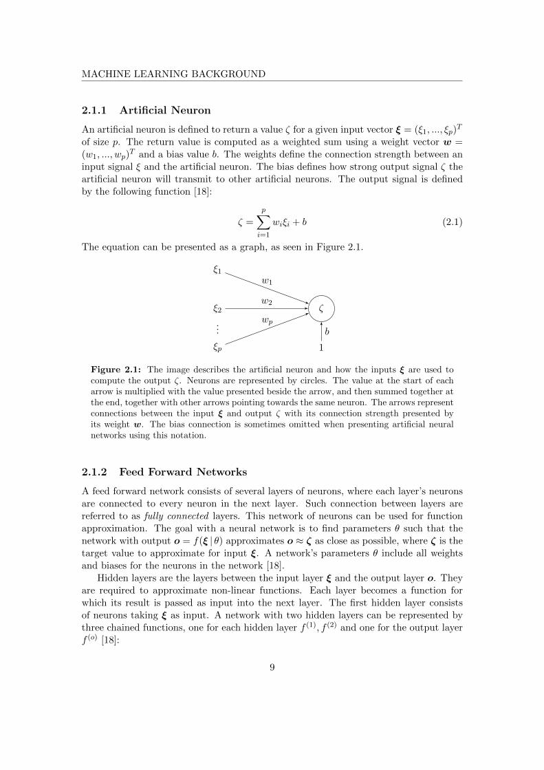
An artificial neuron is defined to return a value ζ for a given input vector ξ = (ξ1, ..., ξp)T
of size p. The return value is computed as a weighted sum using a weight vector w =(w1, ..., wp)
T and a bias value b. The weights define the connection strength between aninput signal ξ and the artificial neuron. The bias defines how strong output signal ζ theartificial neuron will transmit to other artificial neurons. The output signal is definedby the following function [18]:
ζ =
p∑i=1
wiξi + b (2.1)
The equation can be presented as a graph, as seen in Figure 2.1.
ζ
ξ1
ξ2
...
ξp 1
w1
w2
wpb
Figure 2.1: The image describes the artificial neuron and how the inputs ξ are used tocompute the output ζ. Neurons are represented by circles. The value at the start of eacharrow is multiplied with the value presented beside the arrow, and then summed together atthe end, together with other arrows pointing towards the same neuron. The arrows representconnections between the input ξ and output ζ with its connection strength presented byits weight w. The bias connection is sometimes omitted when presenting artificial neuralnetworks using this notation.
2.1.2 Feed Forward Networks
A feed forward network consists of several layers of neurons, where each layer’s neuronsare connected to every neuron in the next layer. Such connection between layers arereferred to as fully connected layers. This network of neurons can be used for functionapproximation. The goal with a neural network is to find parameters θ such that thenetwork with output o = f(ξ | θ) approximates o ≈ ζ as close as possible, where ζ is thetarget value to approximate for input ξ. A network’s parameters θ include all weightsand biases for the neurons in the network [18].
Hidden layers are the layers between the input layer ξ and the output layer o. Theyare required to approximate non-linear functions. Each layer becomes a function forwhich its result is passed as input into the next layer. The first hidden layer consistsof neurons taking ξ as input. A network with two hidden layers can be represented bythree chained functions, one for each hidden layer f (1), f (2) and one for the output layerf (o) [18]:
9

MACHINE LEARNING BACKGROUND
o = f(ξ | θ) = f (o)(f (2)
(f (1)(ξ | θ) | θ
)| θ)
When a network has several layers, an activation function g is used to computethe hidden values between the layers. An activation function must be monotonic anddifferentiable. When using activation functions and at least one hidden layer, a neuralnetwork can approximate any non-linear function [19]. The output of a neuron in the
first hidden layer h(1) = (h(1)1 , . . . , h
(1)n )T is computed as in Equation 2.2. The superscript
of h(l) denotes the layer.
h(1)j = g
(p∑i=1
w(1)ji ξi + b
(1)j
)(2.2)
The weight values w(1)ji becomes a matrix W (1) weighting each component of ξ to
each component of h(1), and bias values b(1)j becomes the vector b(1) representing the
threshold for each neuron in the hidden layer h(1):
W (1) =
w
(1)11 w
(1)12 . . . w
(1)1p
w(1)21 w
(1)22 . . . w
(1)2p
......
. . ....
w(1)n1 w
(1)n2 . . . w
(1)np
b(1) =
b(1)1
b(1)2...
b(1)n
Using matrix notation, Equation 2.2 is equivalent to:
h(1) = g(W (1)ξ + b(1)
)Two examples of activation functions are the sigmoid function that transforms x into
a value between 0 and 1, or tanh returning a value between -1 and 1.
sigmoid: g(x) = 11+e−x : R→ (0,1)
tanh: g(x) = tanh(x) : R→ (−1,1)
The output vector o = (o1, ..., on)T is computed using the values from the last hidden
layer h(d−1) = (h(d−1)1 , ..., h
(d−1)q )T , where d is the depth of the neural network:
10

MACHINE LEARNING BACKGROUND
ok =g
q∑j=1
w(d)kj h
(d−1)j + b
(d)k
o =g
(W (d)h(d−1) + b(d)
)A neural network with two hidden layers can be expressed as in Equation 2.3 and
2.4. The same neural network is also presented in Figure 2.2 as a graph.
ok =g(o)
j∑j′=1
w(o)kj′g
(2)
i∑i′=1
w(2)j′i′g
(1)
p∑p′=1
w(1)i′p′ξp′ + b
(1)i′
+ b(2)j′
+ b(o)k
(2.3)
o =g(o)(W (o)g(2)
(W (2)g(1)
(W (1)ξ + b(1)
)+ b(2)
)+ b(o)
)(2.4)
ξ1
ξ2
...
ξp
ξ
h(1)1
h(1)2
...
h(1)i
h(1)
h(2)1
h(2)2
...
h(2)j
h(2)
o1
o2
...
ok
oW (1) W (2) W (o)
Figure 2.2: A neural network representing a function f(ξ|θ) = o, with two hidden layers;h(1), with i hidden neurons, and h(2), with j hidden neurons, where f : Rp → Rk andθ =
(W (1), b(1)
),(W (2), b(2)
),(W (o), b(o)
). Biases are omitted in this figure.
2.1.3 Optmizing Neural Networks
The neural network parameters θ are learned by minimizing a loss function L(θ). The lossfunction give a value for how large the difference is between the network’s approximationo(µ) and the target value ζ(µ) it approximates, where µ identifies a training instance.Sum of squared errors, one of many loss functions, is used. With N number of instancesto approximate, where the superscript denotes the instance, the loss function is definedby [18]:
11

MACHINE LEARNING BACKGROUND
L(θ) =1
2N
N∑µ=1
||o(µ) − ζ(µ)||2 (2.5)
where o(µ) = f(ξ(µ)|θ)
2.1.4 Gradient Descent
The network parameters θ that minimize L(θ) are found by computing the gradients ofL with respect to θ, ∇θL(θ), for all instances in the training set. The weights and biasesare iteratively updated in the direction of the negative gradient, with a small learningrate 0 < η 1 [20]:
θt = θt−1 − η∇θt−1L(θt−1) (2.6)
where t is the training iteration. Batch gradient descent, as the method is called, isproven to converge to the global minimum only on convex problems, which neural net-works typically are not [18]. Calculating the gradients using batch gradient descent canalso be slow for large datasets. Many training instances can be similar, which makessome gradient computations in every update redundant. Instead, the gradients can becalculated for a sampled set of training instances, using Stochastic Gradient Descent(SGD). Let the sample size of training instances be B ∈ [1,N ]. The update formula forSGD is then given by [18]:
θt = θt−1 − η∇θt−1L(θt−1 |
(ξ(1), ζ(1)), ..., (ξ(B), ζ(B))
)SGD updates have a higher variance than the batch gradient descent update. This
means that L(θ) can fluctuate, which increases the chance of not getting stuck in a poorlocal minimum. However, the global minimum will also be more difficult to converge to.By decreasing the learning rate over time the variance can be reduced [18].
2.1.5 Backpropagation
Backpropagation is an algorithm for computing derivatives for L(θ) with respect to θ.With these derivatives, an optimization method such as gradient descent is used toupdate the network’s weights and biases to minimize L(θ). The gradients are partialderivatives for L(θ) with respect to each weight and bias parameter. Equation 2.6 from
gradient descent can be applied for a single weight parameter w(l)ji , which creates the
update rule for that weight [21]:
w(l)ji,t = w
(l)ji,t−1 − η
∂L
∂w(l)ji,t−1
The partial derivative of w(l)ji in layer l is defined using the chain rule as:
12
MACHINE LEARNING BACKGROUND
∂L
∂w(l)ji
=∂L
∂h(l)j
∂h(l)j
∂w(l)ji
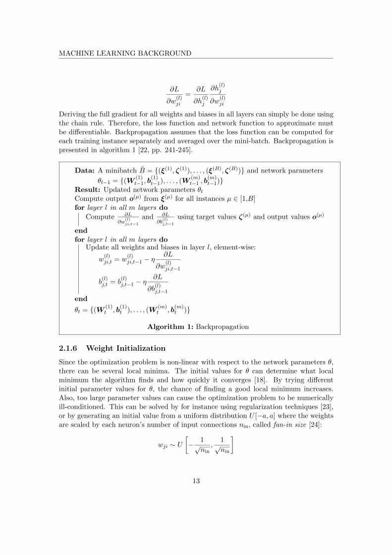
Deriving the full gradient for all weights and biases in all layers can simply be done usingthe chain rule. Therefore, the loss function and network function to approximate mustbe differentiable. Backpropagation assumes that the loss function can be computed foreach training instance separately and averaged over the mini-batch. Backpropagation ispresented in algorithm 1 [22, pp. 241-245].
Data: A minibatch B = (ξ(1), ζ(1)), . . . , (ξ(B), ζ(B)) and network parameters
θt−1 = (W (1)t−1, b
(1)t−1), . . . , (W
(m)t−1 , b
(m)t−1)
Result: Updated network parameters θtCompute output o(µ) from ξ(µ) for all instances µ ∈ [1,B]for layer l in all m layers do
Compute ∂L
∂w(l)ji,t−1
and ∂L
∂b(l)j,t−1
using target values ζ(µ) and output values o(µ)
endfor layer l in all m layers do
Update all weights and biases in layer l, element-wise:
w(l)ji,t = w
(l)ji,t−1 − η
∂L
∂w(l)ji,t−1
b(l)j,t = b
(l)j,t−1 − η
∂L
∂b(l)j,t−1
end
θt = (W (1)t , b
(1)t ), . . . , (W
(m)t , b
(m)t )
Algorithm 1: Backpropagation
2.1.6 Weight Initialization
Since the optimization problem is non-linear with respect to the network parameters θ,there can be several local minima. The initial values for θ can determine what localminimum the algorithm finds and how quickly it converges [18]. By trying differentinitial parameter values for θ, the chance of finding a good local minimum increases.Also, too large parameter values can cause the optimization problem to be numericallyill-conditioned. This can be solved by for instance using regularization techniques [23],or by generating an initial value from a uniform distribution U [−a, a] where the weightsare scaled by each neuron’s number of input connections nin, called fan-in size [24]:
wji ∼ U[− 1√nin
,1√nin
]
13
MACHINE LEARNING BACKGROUND
2.1.7 Recurrent Networks
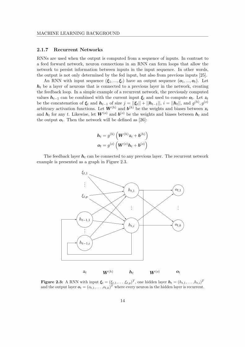
RNNs are used when the output is computed from a sequence of inputs. In contrast toa feed forward network, neuron connections in an RNN can form loops that allow thenetwork to persist information between inputs in the input sequence. In other words,the output is not only determined by the fed input, but also from previous inputs [25].
An RNN with input sequence (ξ1, ..., ξt) have an output sequence (o1, ...,ot). Letht be a layer of neurons that is connected to a previous layer in the network, creatingthe feedback loop. In a simple example of a recurrent network, the previously computedvalues ht−1 can be combined with the current input ξt and used to compute ot. Let ztbe the concatenation of ξt and ht−1 of size j = ||ξt|| + ||ht−1||, i = ||ht||, and g(h), g(o)
arbitrary activation functions. Let W (h) and b(h) be the weights and biases between ztand ht for any t. Likewise, let W (o) and b(o) be the weights and biases between ht andthe output ot. Then the network will be defined as [26]:
ht = g(h)(W (h)zt + b(h)
)ot = g(o)
(W (o)ht + b(o)
)The feedback layer ht can be connected to any previous layer. The recurrent network
example is presented as a graph in Figure 2.3.
ξt,1
...
ξt,p
ht−1,1
...
ht−1,i
zt
ht,1
...
ht,i
ht
ot,1
...
ot,k
otW (h) W (o)
Figure 2.3: A RNN with input ξt = (ξt,1, . . . ,ξt,p)T , one hidden layer ht = (ht,1, . . . ,ht,i)
T
and the output layer ot = (ot,1, . . . ,ot,k)T where every neuron in the hidden layer is recurrent.
14

MACHINE LEARNING BACKGROUND
When running backpropagation on a recurrent network, the network needs to beunrolled a fixed number of steps in order to calculate the derivatives. Unrolling canbe seen as copying the part of the network that exists within the loop, and placingthe copies in a sequence, each connected to the next one. The last unrolled step, h1 =(h1,1 . . . h1,i)
T , will contain some inputs with no values. To solve this, these values can beinitialized with a default value of 0. An unrolled RNN over three time steps is presentedin Figure 2.4. Calculating derivatives for backpropagation is then no different than fora feed forward network [25].
ξ1,1
...
ξ1,p
h1,1
...
h1,i
o1,1
...
o1,k
ξ2,1
...
ξ2,p
h2,1
...
h2,i
o2,1
...
o2,k
ξ3,1
...
ξ3,p
h3,1
...
h3,i
o3,1
...
o3,k
ξt W (1) ht W (o) ot
ξ1
ξ2
ξ3
h1
h2
h3
o1
o2
o3
Figure 2.4: To the left; an unfolded RNN, where every neuron in the hidden layer isrecurrent. The network is unfolded three time steps, with input ξt = (ξt,1, . . . ,ξt,p), onehidden layer ht = (ht,1, . . . ,ht,i) and the output layer ot = (ot,1, . . . ,ot,k), where t is thetime step. Note that the same network weights are used each time step. The same neuralnetwork is presented on the right, where each box represents a neural network layer, andeach arrow represents input and output data used by the layer.
15

MACHINE LEARNING BACKGROUND
2.1.8 Long Short-Term Memory
An LSTM is a recurrent network constructed for tasks with long-term dependencies. Aregular RNN struggle to remember longer sequences due to vanishing gradients, whichmeans that the gradients decrease exponentially for each unrolled time step. This is notthe case for LSTM networks, due to their internal structure. LSTM networks attempt tomimic a Turing complete machine, by storing memory in cells, and modify this memoryby using insert and forget gates. During training, the network learns how to controlthese gates. As a result of this, both newly seen observations and observations seen along time ago can be stored and used by the network [27].
A hidden layer in an LSTM consists of four fully connected internal layers thattogether creates an output ht and an internal cell state Ct, which are both rememberedbetween observations. The cell state is modified by inserting data to it or by removingremembered data. Two of the internal layers are the forget gate layer ff and the insertgate layer fi. They both return a vector containing values between 0 and 1, where eachvalue describes how important that element is in Ct. For the forget layer, a 1 will keepthe remembered data and a 0 will forget it. The layers are using a sigmoid activationfunction σ(x) and will later be used for an element-wise multiplication (denoted by )with the cell state [27]:
ff = σ(Wfzt + bf )
fi = σ(Wizt + bi)
A candidate for the new cell state, Ct, is computed from zt = (ξt ||ht−1), where ||denotes a concatenation. The cell state Ct is updated by passing the old cell state Ct−1
through the forget gate and the candidate cell state C through the insert gate [27]:
Ct = tanh(WCzt + bC)
Ct = ff Ct−1 + fi Ct
The output of the cell, ht, contains selected values from the cell state. Anothersigmoid layer, fo, is used to filter what parts of Ct to include in the output [27]:
fo = σ(Wozt + bo)
ht = fo tanh(Ct)
A memory for Ct and ht stores these values for the next observation. A networkcan contain multiple LSTM cell layers. In that case, each cell has its own memoryand computes ht based on its own Ct−1 and ht−1. The parameters for an LSTM cellare θ = Wf ,Wi,WC ,Wo, bf , bi, bC , bo, which are trained using backpropagation byunrolling each layer over time, similar to a normal RNN [27]. A graphical representationfor an LSTM is presented in Figure 2.5.
16

MACHINE LEARNING BACKGROUND
ξt ot
ff fi Ct fo
×
× +
×
tanh
Ct−1
ht−1
Ct
htzt
Figure 2.5: The internal structure of an LSTM cell. The picture shows how to take theinput ξt, the previously hidden state ht−1 and the previous cell state Ct−1, and computethe output ot, the new hidden state ht, and the new cell state Ct. Two merging arrowsdenotes a concatenation. Two splitting arrows propagate the same data to every output.Circles denotes a simple mathematical operation. A rectangle represents a fully connectedneural network layer.
2.1.9 Dropout to Prevent Overfitting
Overfit neural networks have bad generalization performance [28]. Dropout is used tohelp reduce overfitting. The idea with dropout is to temporarily remove random hiddenneurons with their connections from the network, before each training iteration. This isdone by, independently, for each neuron, setting its value to 0 with a probability p [29].Let m(l) be a mask where each element is 1 with probability p and 0 otherwise. Thefunction for a hidden layer defined in section 2.1.2 is updated to the following equation:
h(l) = m(l) g(W (l)ξ + b(l)
)The backpropagation algorithm is updated accordingly. A network used in a training
iteration will contain a subset of the neurons from the full neural network. There are anexponential number of these subsets, and backpropagation with dropout can be seen asan algorithm training all those sub-networks. The final network will become an averageof all sub-networks. During validation, all neurons are present but their weights aremultiplied by p. This makes the expected output of the network during validation thesame as during training [29].
2.2 Reinforcement Learning
This section introduces the Markov Decision Process (MDP) model followed by thefundamental framework of reinforcement learning, as well as explanations to explorationand exploitation. Thereafter, Deep Q-Learning algorithm and its stability issues arepresented, together with how to solve them. Partially Observable Markov Decision
17
MACHINE LEARNING BACKGROUND
Process (POMDP), an extension to MDP, is introduced. At last, DRQN is presented,which extends DQN for partially observable environments by using a POMDP.
2.2.1 Markov Decision Process
Reinforcement learning algorithms described in this chapter require the problem to bemodeled as a MDP.
Definition 1. An MDP for some environment E is described by a 5-tuple(S,A,P,R, γ), where S is the finite state space, A is the finite action space, Pis the transition probability distribution for traversing from state st ∈ S to anotherstate st+1 ∈ S given an action at ∈ A. The reward rt = R(st, at) ∈ R is thereal-valued immediate rewards, given that action at was taken at state st. The lastparameter γ ∈ (0, 1], which is the discount factor, is used to weight short term andlong term rewards.
The MDP model assumes that a state st+1 only depends on the previous state st andaction at. This is known as the Markov property [30].
2.2.2 Reinforcement Learning Framework
Reinforcement learning is an optimization problem where an agent learns a policy bytrial and error. Using the MDP model, an agent receives an observation ot at time t froman environment E . These observations can be fully observable or partially observable ofthe full environment. The environment could be deterministic or stochastic. From a setof observations, a state st is constructed, e.g st = f(o0, o1, ..., ot) for some function f .The agent chooses an action at, given the state. The action impacts the environment tosome degree, which is then used to obtain a new observation ot+1 and construct anotherstate st+1. Some states are terminating states, meaning they have no outgoing actions,and no new states can be constructed [31]. In order to capture both stochastic anddeterministic environments, a transition function; TE(st,at,st+1) ∼ P is used to describethe probability to transition from state st to st+1 given that action at was taken.
To determine whether an action is good or bad, the agent receives a reward rt =R(st,at) after choosing an action at in a state st. The reward function returns either apositive value to reward the agent when choosing good actions, or a negative value topunish it. The agent tries to maximize the reward it gets. The function R(st,at) mustbe defined in the model before the learning starts. The definition of the reward functionR(st,at) influences the behavior of the learned policy, as it defines the goal of the task.
A policy π defines the behavior of an agent, by specifying what actions the agenttakes. The goal of reinforcement learning is to converge towards the optimal policy π∗.A policy function can be modeled in two ways:
18

MACHINE LEARNING BACKGROUND
• A deterministic policy π : S → A, is a function describing which action the agentwill take, given a state.
• A stochastic policy π : S × A → [0,1], is a function describing the probability fortaking an action given a state.
In order to learn the optimal policy, two functions; Vπ : S → R and Qπ : S × A → Rare used. The value function; Vπ(st), describes the expected future reward given a statest using policy π. The action value function; Qπ(st,at), describes the expected futurereward for taking an action at in a state st using the same policy. Comparing Qπ(st,at)to the reward function R(st,at), the functions are similar, except the Qπ-function alsotakes expected future rewards into consideration.
The optimal policy π∗ takes actions according to an optimal Qπ(st,at) function,denoted Qπ∗(st,at). The policy π is updated by iteratively reevaluating all Qπ-valuesaccording to the following Bellman equation, resulting in a new policy π′:
Qπ′(st,at) = rt + γ∑
st+1∈STE(st,at,st+1)Vπ(st+1) (2.7)
where Vπ(st) is the value function for the old policy π, defined as:
Vπ(st) = maxat
Qπ(st,at)
For a policy π, actions are taken according to the highest Qπ-value [32]:
π(st) = arg maxat
Qπ(st,at)
When the Qπ-function is iteratively updated, Qπ → Qπ∗ as the number of updates goesto infinity [32].
2.2.3 Exploration and Exploitation
The agent takes actions by exploiting the knowledge it has previously gained, by choosingactions according to its policy. By only exploiting its policy, the agent explores a limitedset of states in the environment. There can be unexplored states that give a higherreward unknown to the current policy. By using ε-greedy, the agent chooses a randomaction with probability ε and otherwise follows the policy, thus utilizing exploration.The balance between exploration and exploitation can be adjusted by setting ε. In thebeginning of a training session, ε is close to 1, and then decreased over time [31].
2.2.4 Deep Q-Learning
This section presents the Deep Q-Learning algorithm. Two solutions handling stabil-ity issues with Deep Q-Learning, experience replay and fixed target network, are alsoexplained.
19

MACHINE LEARNING BACKGROUND
2.2.4.1 Deep Q-Learning Algorithm
The Deep Q-Learning algorithm is a reinforcement learning algorithm that uses a neuralnetwork as a function approximator for the Qπ-function [10]. This neural network iscalled DQN. The Qπ-function approximated by the DQN is denoted as Q(st,at|θπ),where θπ are the neural network parameters for policy π. When using a DQN, thereward function is optimally distributed around [−1, 1]. If the defined reward values aretoo large, the Qπ values can become large and cause the gradients to grow [33].
Deep Q-Learning is a model-free reinforcement learning algorithm, which means thatthe transition function TE(st,at,st+1) for the MDP is unknown. By conducting exper-iments and receiving experiences e from the environment E , the transition functionTE(st,at,st+1) is embedded inside the Qπ values. Actions are taken according to theε-greedy strategy, and experiences from taken actions are recorded [10]. An experiencee is defined as a tuple of the current state st, taken action at, observed reward rt andthe new state st+1; e = (st,at,rt,st+1). These experiences are stored in an experiencememory E and are used for training the neural network. The neural network trains itsweights and biases θπi , where πi is the policy for training iteration i. In order to trainthe DQN, Qtargeti is computed from an experience, which is the real immediate rewardand predicted future rewards for iteration i, derived from Equation 2.7:
Qtargeti =
rt if st is terminating the episode
rt + γmaxat+1 Q(st+1, at+1|θ−) otherwise
A separate set of network parameters θ−, which are computed from θπi−1 , is used forcomputing Qtargeti . This is called a fixed target network, and is introduced to makeQtargeti independent from θπi to make DQN updates more stable [11]. How to set thetarget network parameters θ− is found in Section 2.2.4.3.
The loss function L(θπi), for a DQN with network parameters θπi , measures the dif-ference between the real reward and the DQN’s predicted reward, which is implementedby computing the sum of squared errors between Q(st,at|θπi) and Qtargeti [10]:
L(θπi) =1
2N
∑(st,at)∼ρπ
(Q(st, at|θπi)−Qtargeti
)2(2.8)
where ρπ is a probability distribution over states st and actions at for policy π, which isused to sample N state and action pairs from the experience memory E. Using the lossfunction, the following gradient is computed, which is the gradient used when performingbackpropagation on the DQN [10]:
∇θπiL(θπi) =1
N
∑(st,at)∼ρπ ;st+1∼E
(Q(st, at|θπi)−Qtargeti
)∇θπiQ(st, at|θπi) (2.9)
The Deep Q-Learning algorithm, using a fixed target Q-network, is presented below[10].
20
MACHINE LEARNING BACKGROUND
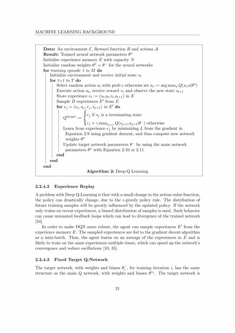
Data: An environment E , Reward function R and actions AResult: Trained neural network parameters θπ
Initialize experience memory E with capacity NInitialize random weights θπ = θ− for the neural networksfor training episode 1 to M do
Initialize environment and receive initial state s1
for t=1 to T doSelect random action at with prob ε otherwise set at := arg maxaQ(st,a|θπ)Execute action at, receive reward rt and observe the new state st+1
Store experience et := (st,at,rt,st+1) in ESample B experiences E′ from Efor ej = (sj , aj , rj , sj+1) in E′ do
Qtarget :=
rj if sj is a terminating state
rj + γmaxaj+1 Q(sj+1,aj+1|θ−) otherwiseLearn from experience ej by minimizing L from the gradient inEquation 2.9 using gradient descent, and thus compute new networkweights θπ
Update target network parameters θ− by using the main networkparameters θπ with Equation 2.10 or 2.11
end
end
endAlgorithm 2: Deep-Q Learning
2.2.4.2 Experience Replay
A problem with Deep Q-Learning is that with a small change in the action-value function,the policy can drastically change, due to the ε-greedy policy rule. The distribution offuture training samples will be greatly influenced by the updated policy. If the networkonly trains on recent experiences, a biased distribution of samples is used. Such behaviorcan cause unwanted feedback loops which can lead to divergence of the trained network[34].
In order to make DQN more robust, the agent can sample experiences E′ from theexperience memory E. The sampled experiences are fed to the gradient decent algorithmas a mini-batch. Thus, the agent learns on an average of the experiences in E and islikely to train on the same experiences multiple times, which can speed up the network’sconvergence and reduce oscillations [10, 35].
2.2.4.3 Fixed Target Q-Network
The target network, with weights and biases θ−i , for training iteration i, has the samestructure as the main Q network, with weights and biases θπi . The target network is
21

MACHINE LEARNING BACKGROUND
updated at a slower pace than the main network, which reduce oscillations [11]. Twodifferent update strategies for the target network’s parameters can be used:
1. With interval C: θ−i = θπi (2.10)
2. Every network update: θ−i = τ · θ−i−1 + (1− τ) · θπi (2.11)
where i is the update iteration. For the interval update (1), C determines how frequentlythe target network is updated. A smooth update (2) can also be used, where τ representshow much to interpolate the target network for the last update with the current mainnetwork [11, 36].
2.2.5 Partial Observability
DQN relies on the MDP model described in Definition 1. When dealing with partiallyobservable environments, a model can be constructed by using a partially observableMDP model. The problem is still assumed to be an MDP, except that parts of the stateare hidden from the agent [14].
Definition 2. A POMDP for some environment E is described by a 6-tuple(S,A,P,R,Ω, O), where S, A, P and R represents an MDP. An observation ot ∈ Ωis observed, where Ω is the finite observation space. Finally, O(st) is the proba-bility distribution for receiving observation ot given an underlying hidden state st:ot ∼ O(st).
2.2.6 Deep Recurrent Q-Network
A DRQN is a DQN with an LSTM cell added after the last hidden layer, before theoutput layer, enabling support for POMDP environments [12]. The LSTM layer addsa recurrence over time, such that the network’s output for observation ot depends on ahistory of previously seen observations. The LSTM’s internal cell state keeps informationabout this observation history. Thus, only the current observation ot needs to be fed tothe network to make a prediction. By using a history of observations, DRQN can betterestimate the underlying system state of the POMDP. The internal cell state is reset tozeros at the start of a new episode.
A DRQN is trained by feeding a sequence of observations ot−l+1, . . . , ot to the un-rolled neural network, where l is the sequence length, and ot+1 as the next observation.The LSTM’s internal cell state is not stored in the experience memory, as it is depen-dent of the network parameters θ. An experience is redefined to contain sequences ofobservations, actions and rewards; e = (ot−l+1 . . . ot, at−l+1 . . . at, rt−l+1 . . . rt, ot+1) [12].Before each training update, the LSTM’s internal state is zeroed. This method preserverandom sampling from the experience memory, described in Section 2.2.4.2, which makesthe recurrent update stable.
22

MACHINE LEARNING BACKGROUND
This method is extended by using the first h observations of an experience to buildthe LSTM layer’s cell state. Only the rest of the observations, ot−l+h+1, . . . , ot, aretrained on [37]. Figure 2.6 visualizes how these observations are used.
ξt−l+1 ξt−l+h ξt−l+h+1 ξt
0 ht−l+1 . . . ht−l+h ht−l+h+1 . . . ht
ot−l+1 ot−l+h ot−l+h+1 ot
build hidden state
train
Figure 2.6: Use h number of observations in a sequence to build the LSTM’s cell state.The rest l−h number of observations are trained on. The observations are fed as inputs ξt.The initial cell state of ht−l+1 is zero.
23

3Traffic Simulator for Crossings
This chapter describes the fundamental mechanics of the simulator. This includes anepisode’s terminating conditions. The coordinate system for lanes is defined togetherwith how lanes relate to each other in the coordinate system. Furthermore, the repre-sentation of curved lanes is explained. Thereafter, the parameters that the car modeluse, as well as its mechanics are presented. At last, the agents that drives target carsare presented.
3.1 Episode Timeframe
Each time the traffic simulator starts a new episode, it initializes a traffic scenario withcars and lanes, as described in Section 1.4.1. The episode ends when one of the followingterminating conditions are fulfilled:
• The ego car has successfully arrived at its target destination along the lane, spec-ified in the traffic scenario.
• The ego car has collided with another car. A vehicle is shaped like a rectangle, andoverlapping of two such rectangles results in a collision between the two vehicles.
• A timeout has occurred; t > tm where t is the current time from the start of thecurrent episode, and tm is the maximum amount of time allowed for that episode,specified by the scenario.
3.2 Coordinate System for Lanes
A coordinate system 1 models crossings and merging lanes, such as the scenarios de-scribed in section 1.3. A lane L is defined as a sequence of coordinates L := (ψ1 =
1The coordinate system is proposed by Mohammad Ali at Zenuity.
24

TRAFFIC SIMULATOR FOR CROSSINGS
(x1,y1),ψ2 = (x2,y2), . . . ) and a lane width w(L), constructing a sequence of straightlane segments that cars can drive on. A lane segment is denoted as (ψi,ψi+1);ψi ∈L ∧ψi+1 ∈ L. An illustration of a lane and its lane segments is presented in Figure 3.1.An intersection point between two lanes L and L′ is denoted by ψ× and exists if the twolanes have a common point:
ψ× ∈ L ∧ψ× ∈ L′
ψi−1
ψi
ψi+1
Segment (ψi,ψi+1) w(L)
Figure 3.1: An illustration of three con-secutive points ψi−1,ψ1 and ψi+1 for a laneL. The lane has two segments with one ofthe segments (ψi,ψi+1) explicitly shown atthe end of the dotted arrow. The lane widthw(L) is also shown in the figure.
The longitudinal position along a lane is described by φ(L)i where i identifies a point
ψi along the lane L. The longitudinal position up to a certain point along the lane isdefined recursively as follows:
φ(L)1 = 0
φ(L)i = ||ψi −ψi−1||+ φ
(L)i−1
The lane length is φ(L)l where l identifies the last point ψl on the lane. For any point ψ,
its longitudinal position along the lane L is described by φ(L), and can be any number
in the interval [0,φ(L)l ]. All lanes have a driving direction which increase longitudinal
positions as the car moves forward along the lane. Cars can only traverse forward onlanes. A car’s longitudinal position can be described from lanes other than its currentlane. Let Lc denote the current lane for a car c, and let Lo denote another lane. Then,the car has a longitudinal position along lane Lo if and only if there exists an intersectionpoint ψ× between the two lanes, and this point is ahead of the car. Formally:
ψ× ∈ Lc ∧ψ× ∈ Lo ∧ φ(Lc)× ≥ p(c,Lc)
t
where p(c,Lc)t denotes the longitudinal position of the car c along its lane Lc at time step
t, and φ(Lc)× is the longitudinal position of the intersection point between the lanes Lc
and Lo along the lane Lc. When a longitudinal position of car c on another lane Lo iscalculated, the first intersection point is always used. If there are multiple intersection
25

TRAFFIC SIMULATOR FOR CROSSINGS
points, the two lanes merge. The first intersection point is the one with the lowest
longitudinal position φ(L)× . Figure 3.2 (left) presents two intersecting lanes with multiple
intersection points, and shows the first and the last intersection points. The car c’s
position along another lane Lo, p(c,Lo)t , is calculated such that the longitudinal distance
to the first intersecting point ψ× is the same on both lanes Lc and Lo, by using Equation3.1. Figure 3.2 (right) displays an example of the longitudinal position of the same caron two different intersecting lanes.
p(c,Lo)t = φ
(Lo)j − φ(Lc)
i + p(c,Lc)t ; ψi ∈ Lc,ψj ∈ Lo,ψi = ψj (3.1)
ψi−1ψj−1
ψi = ψj = ψ×
ψi+1 = ψj+1
ψi+2 = ψj+2 = ψ′×
ψi+3ψj+3
ψi−1
ψi = ψj = ψ×
ψi+1
Lo
ψj−1
ψj+1
Lc
p(Lc)
p(Lo)
Figure 3.2: Left figure: Two lanes merge and then diverge again. There exists threeintersection points between the two lanes, where the first intersection point is denoted ψ×and the last intersection point is denoted ψ′×. Right figure: Two lanes Lc and Lo intersect
at ψ×. A car c in front of the intersection has a position p(Lc) on lane Lc and p(Lo) on laneLo
In order to determine if any point ψ is on a specific lane, ψ is projected onto everysegment of the lane. If the distance between the original point ψ and the projectedpoint is less than half the lane width w(L), the point is considered to be on the lane. An
overlap point ψ(L) is defined between two lanes L and L′ if and only if there exists at
least one point ψ that is on both lanes. The overlap point for lane L is the projectedpoint from the set of all points on both lanes with the lowest longitudinal position. Let
φ(L) denote the longitudinal position of such a projected point, then
φ(L) = minφ(L)
where φ(L) comes from the set of all projected longitudinal positions, which are projectedfrom every point ψ that are on both the lanes L and L′. Figure 3.3 presents two lanes,with the set of all points that are on both lanes (potential overlap points, marked in
grey) as well as the overlap point ψ(L) .
26
TRAFFIC SIMULATOR FOR CROSSINGS
ψi−1
ψ×
ψi+1
ψj−1
ψj+1
ψ(L)
φ(L)
Figure 3.3: Two overlapping lanes L and L′.The grey area is the set of all points which areconsidered on both lanes. The overlapping point
ψ(L) for lane L is presented at the center of a
circle. The longitudinal distance of the overlap
point along the lane L; φ(L) is also presented.
Note that the overlap point for lane L′; ψ(L′)
might not always be the same point as ψ(L) .
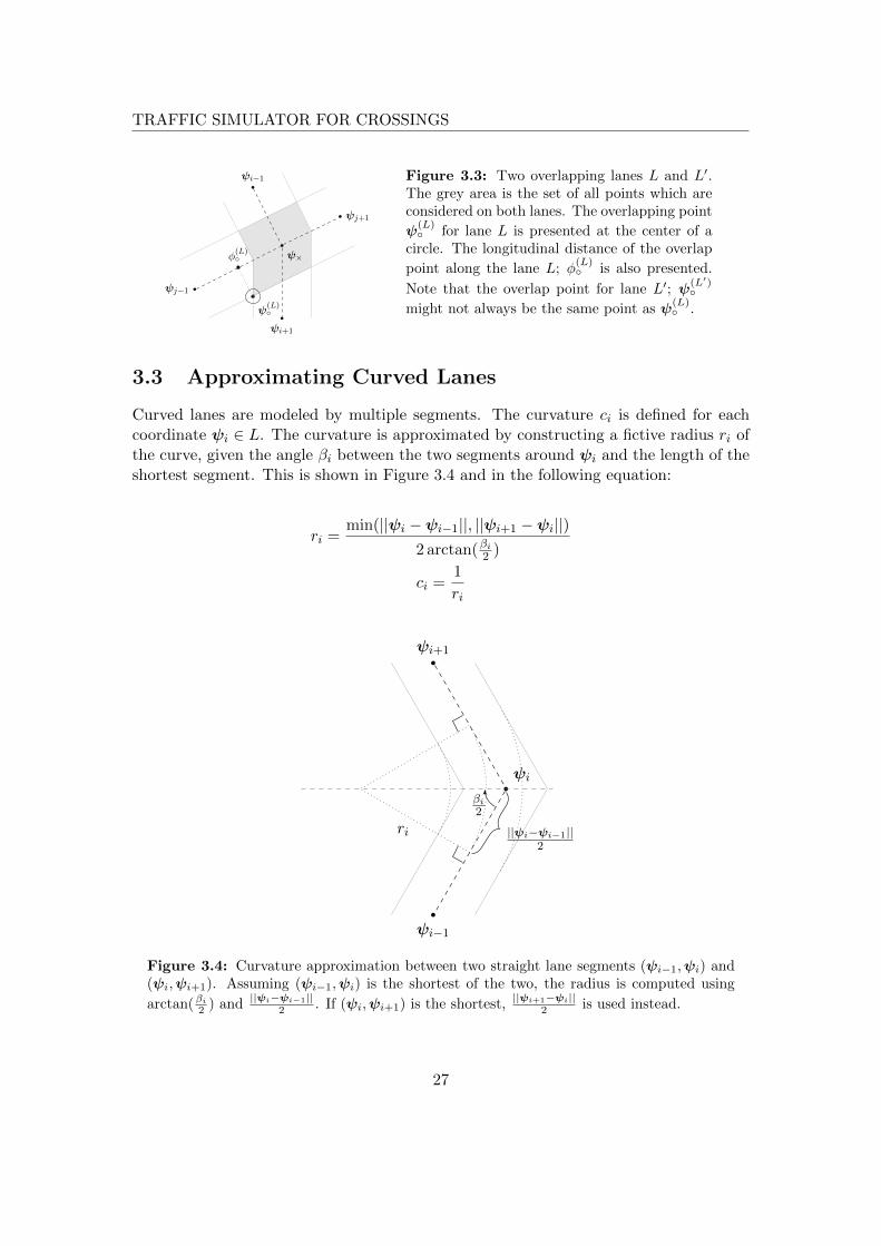
3.3 Approximating Curved Lanes
Curved lanes are modeled by multiple segments. The curvature ci is defined for eachcoordinate ψi ∈ L. The curvature is approximated by constructing a fictive radius ri ofthe curve, given the angle βi between the two segments around ψi and the length of theshortest segment. This is shown in Figure 3.4 and in the following equation:
ri =min(||ψi −ψi−1||, ||ψi+1 −ψi||)
2 arctan(βi2 )
ci =1
ri
ri
ψi
ψi−1
||ψi−ψi−1||2
ψi+1
βi2
Figure 3.4: Curvature approximation between two straight lane segments (ψi−1,ψi) and(ψi,ψi+1). Assuming (ψi−1,ψi) is the shortest of the two, the radius is computed using
arctan(βi
2 ) and ||ψi−ψi−1||2 . If (ψi,ψi+1) is the shortest, ||ψi+1−ψi||
2 is used instead.
27
TRAFFIC SIMULATOR FOR CROSSINGS
3.4 Car Model
A vehicle c is described by these parameters at time t:
p(c)t :
The longitudinal position of the vehicle along its lane, positioned at the
rear axle.
v(c)t : The speed along the direction of the vehicle.
a(c)t : The acceleration along the direction of the vehicle.
s(c) =
[s
(c)1
s(c)2
]: The width and length of the vehicle.
A vehicle’s position, speed, and acceleration are updated according to the followingequations:
a(c)t+1 = a
(c)t + j
(c)t+1∆t
v(c)t+1 = v
(c)t + a
(c)t+1∆t− 1
2j
(c)t+1∆t2
p(c)t+1 = p
(c)t + v
(c)t+1∆t− 1
2a
(c)t+1∆t2
where j(c)t is the jerk along the lane, defined as j
(c)t := max(min((a
(c)t −a
(c)t )/∆t), jmax,−
jmax), with jmax as max jerk, a(c)t is the desired acceleration, used to control the vehicle,
and ∆t denotes the time between two simulation updates, thus approximating continuoustime with discrete updates. Max jerk jmax is used to limit the acceleration control signal,thus making sure agents are limited by artificial inertia. Whenever a car reach the endof its lane, it is instantly put at the start of the lane, to keep the same number of carsthroughout the episode.
3.5 Car Agents with Different Behaviours
The following agents are defined as drivers for target cars. Each agent have manuallydefined STGs which are passed to the low-level controller. How to compute the desiredacceleration from an STG is defined is described in Section 4.2.2:
• Take way agent. An agent always driving according to the take way STG.
• Give way late agent. The agent initially has the same behavior as the take wayagent, but very late decides to stop at the next crossing using the give way STG.
• Cautious agent. The agent initially has the same behavior as the take way agent,but slows down before the crossing. In contrast to the give way late agent, the agentdoes not stop, and switches to the take way STG when it is close to the crossing.A parameter determining how much the agent slows down when approaching acrossing is configurable, and is referred to as cautiousness.
28
TRAFFIC SIMULATOR FOR CROSSINGS
• Trained agent. An agent using a policy from a previously trained ego agent.The policy of this agent depends on how it was trained. The trained agent differsfrom an ego agent because it cannot further update its policy, and is used to drivetarget cars.
29

4Acceleration Regulator
This chapter discusses the how the Acceleration Regulator works and motivates thealgorithm choices. Both the high- and low-level controller presented in Section 1.3 aredescribed. Furthermore, all the features that the high-level controller base its decisionson are presented. The reward function used to train the high-level controller is presented.At last, the different DQN structures the high-level controller is trained and tested within the Result chapter are presented.
4.1 System Design Choices
As mentioned in Section 1.3, the Acceleration Regulator is divided into a high- and low-level controller. The high-level controller chooses between discrete actions, which the low-level controller use to compute the final acceleration. This architecture enables the high-level controller to use a reinforcement learning algorithm with discrete outputs. A policy-based or an actor-critic method could be used without the need for a low-level controller,as it supports continuous output [38, 39]. However, an approach with discrete outputsreduces the action space, by constraining the possible output acceleration distribution.Also, a model-free reinforcement learning algorithm is necessary to avoid creating amanual model for the MDP of the traffic environment. DQN and DRQN, presented inSections 2.2.4.1 and 2.2.6, are both model-free and use discrete actions. DQN, however,relies on the Markov property assumption, which [14] argue does not hold for trafficenvironments. DRQN solves this problem by using a POMDP environment instead ofan MDP [12]. Both DQN and DRQN are chosen as implementation for the high-levelcontroller, and compared to see if POMDP is necessary.
30

ACCELERATION REGULATOR
4.2 Car Control using the Low-Level Controller
The low-level controller computes a vehicle c’s desired acceleration a(c)t at time t, for an
STG, using regulators. These regulators and how the low-level controller computes thedesired acceleration from STGs, are defined in the following sub-sections.
4.2.1 Regulators
There are three regulators that can be used by the low-level controller, where eachregulator returns an acceleration:
• Cruise Control (CC). Accelerates or decelerates the car to a desired speed vdesired
and then keeps that speed. The regulator function takes a relative speed vrel,t asargument and returns an acceleration:
CC(vrel,t)
where vrel,t = vdesired − v(c)t
• Adaptive Cruise Control (ACC). Used for keeping a desired distance to a selectedtarget, for instance a leading car or a crossing. The car will accelerate or decelerateto reach a relative distance and relative speed of 0 to the target. The regulatortakes a relative distance drange,t and relative speed vrel,t:
ACC(drange,t, vrel,t)
• Curve Speed Adaptation. Limits the speed in a curve. Given curvatures ci (de-scribed in Section 3.3) for all future sample points ψi on the ego lane Lc, themaximum speed for every point is calculated. The maximum longitudinal acceler-ation for the regulator is given by limiting the vehicle’s speed in each sample point,where alat is the maximum allowed lateral acceleration:
CSA(p(c)t , v
(c)t ) = min
iACC
(φ
(Lc)i − p(c)
t ,
√alat
ci− v(c)
t
)where ψi ∈ Lc ∧ φ(Lc)
i > p(c)t
A common notation is used for constraining the vehicle acceleration according to thethree given regulators. If a car c has a leading car l, the acceleration is limited by anACC regulator with the leading car l as target. It also takes the curvature of the laneinto account, in order to make sure that the car does not experience too much lateral
acceleration. The constrained acceleration a(c)t in time step t, is defined as
a(c)t =
min(a, ACC(p
(l)t − p
(c)t − s
(c)2 − doffset, v
(l)t − v
(c)t ))
if leading car exists
a otherwise
(4.1)
31
ACCELERATION REGULATOR
a = min(amax, CC(vmax − v(c)
t ), CSA(p(c)t , v
(c)t ))
where amax denotes the maximum amount of acceleration, vmax is the maximum allowed
speed, doffset is the desired distance to the leading car, and a(c)t denotes the constrained
acceleration for car c.
4.2.2 Low-Level Controller Implementation using Short Term Goals
As seen in Section 1.4.3, the low-level controller use regulators, defined in Section 4.2.1,to adjust the acceleration for a vehicle c according to an STG. It outputs a desired accel-
eration a(c)t , which the car model in Section 3.4 use to update the vehicle’s acceleration
a(c). The low-level controller is defined as follows for each STG:
• Take way. Aims to keep a specified maximum speed vmax, using a CC regulator.
The desired acceleration a(c)t is defined by the constrained acceleration a
(c)t , defined
in Equation 4.1 for a car c:
a(c)t = a
(c)t
• Give way. Stops the car at the next intersection, located at ψi on the car’s lane
Lc. The desired acceleration a(c)t is limited by both the constrained acceleration
a(c)t and an ACC regulator targeted on a stopping point in front of the intersection.
Define the distance to the stopping point as:
d(c)i = φ
(Lc)i − p(c)
t − s(c)2 − dmargin
where dmargin is the distance from the intersection i to the desired stopping point.
The desired acceleration a(c)t is then given by:
a(c)t = min
(a
(c)t , ACC(d
(c)i ,−v(c)
t ))
• Follow vehicle. Using an ACC regulator targeted on a target car o, to keep the same
speed v(o)t and a desired distance doffset to that target car. The desired acceleration
a(c)t is given by:
a(c)t = min
(a
(c)t , ACC(p
(o)t − p
(c)t − s
(c)2 − doffset, v
(o)t − v
(c)t ))
4.3 Actions Chosen by the High-Level Controller
The high-level controller chooses one of 6 actions α1, . . . , α6 ∈ A. As described inSection 1.4.3, an action is defined to be an STG, used by the low-level controller tocompute the desired acceleration. The 6 actions are:
32

ACCELERATION REGULATOR
• α1: Take way STG.
• α2: Give way STG.
• α3: Follow vehicle STG, 1.
• α4: Follow vehicle STG, 2.
• α5: Follow vehicle STG, 3.
• α6: Follow vehicle STG, 4.
The four follow vehicle STG actions, α3, . . . , α6; one for each target car, are used toimprove the ego car’s timing in a crossing or a lane merge. The intended use of the followvehicle action is to follow the traffic flow in the target car’s lane. Each follow vehicleaction is only valid if its target car is visible to the ego agent. The low-level controller’soutput is undefined for invalid follow vehicle actions. If an invalid follow vehicle actionis chosen, the acceleration from the take way action is used instead.
4.4 Selected Features
The features used for the high-level controller’s decision making include features concern-ing the ego car e and up to 4 target cars in the environment. These features representthe MDP state st = (ξ1, . . . , ξp) ∈ S which Deep Q-Learning base its decisions on, de-scribed in Section 2.2.1. As mentioned in Section 1.4.4, there are 32 target features, 8for each target car, and 7 ego features. Motivations for the features are presented afterthe features are defined.
4.4.1 Target features
Target features include all features related to a specific target car c and is repeated foreach car visible to the ego car. Because the features are used as input to a DQN, thenumber of features must be fixed. The features were therefore decided to support upto 4 target cars, as mentioned in Section 1.5, but the approach can support more bysimply expanding the number of target cars. A target car is visible to the ego car ifthe two cars have a common point ψ on their respective lanes, ahead of the ego car:
φ(Le) > p(e)t , where φ(Le) is the longitudinal position of the common point ψ along the
ego lane Le. Thus, target cars driving on already passed lanes are not visible. Thismeans that a traffic scenario can have less than 4 visible target cars, which can leaveempty target features. In such cases, the empty target features are set to -1. All targetfeatures are scaled to be a value between or close to [−1,1] by using a car’s sight rangepmax, maximum speed vmax and maximum acceleration amax.
Let ψ× ∈ Le be the intersection point between the ego lane Le and the target car’s
lane Lc, with the longitudinal position φ(Le)× along the ego lane. Let ψ
(Le) and ψ
(Lc) be
the overlap points for Le and Lc respectively, between the two lanes, with a longitudinal
position of φ(Le) and φ
(Lc) respectively. The target features are listed below:
33
ACCELERATION REGULATOR
• ξ1: Target car’s position relative to ego car, using the target car’s positionalong the ego lane:
p(c,Le)t − p(e)
t
pmax
• ξ2: Target car’s speed,v(c)t
vmax
• ξ3: Ego car’s distance to the first intersection point ψ×. If Lc = Le, thedistance is set to be 0, otherwise:
φ(Le)× − p(e)
t
pmax
• ξ4: Ego car’s speed,v(e)t
vmax
• ξ5: Ego car’s acceleration,a(e)t
amax
• ξ6: Remaining joined distance of ego lane after ψ×. The distance from the
first intersection point φ(Le)× to the last intersection point φ
′(Le)× for lanes Le and
Lc. For a crossing, this value is 0. The distance is calculated from ψ×, or from theego car, if it has passed ψ×,
min
(φ′(Le)× −max(φ
(Le)× , p
(e)t )
pmax, 1
)
• ξ7: Target car’s distance to overlap with ego lane. The distance betweenthe target car and the overlapping point between both lanes along the target car’slane Lc, defined as:
φ(Lc) − p(c)
t
pmax
• ξ8: Ego car’s distance to overlap with target lane. The distance betweenthe ego car and the overlapping point between both lanes along the ego car’s laneLe, defined as:
φ(Le) − p(e)
t
pmax
The first four features ξ1, . . . , ξ4, which include speeds and positions relative to the inter-section point for the ego car and the target car, are included to let the agent infer whenthe cars will arrive at the intersection, which is essential to the problem. The ego car’sacceleration ξ5 is needed to determine how each action will affect the acceleration, whichis essential to minimize jerk. The remaining joined distance ξ6 is used to differentiatewhether the target- and ego lane merge or not. The last two features ξ7 and ξ8 are used
34

ACCELERATION REGULATOR
to determine the distance that the ego car travels on the target lane, in combinationwith ξ3, and vice versa for the target car in combination with ξ1. Figure 4.1 shows anexample of where this is important, since the distance in the turning scenario is longerthan in the straight crossing (as given by ξ7 + ξ1 − ξ3).
Figure 4.1: In a turning scenario (left), the longitudinal distance between the intersection
point ψ× and the target car’s first overlapping point ψ(Lc) is larger than in a straight crossing
(right).
4.4.2 Ego features
The ego features include inputs that are not related to any target cars. These featurestell the ego agent what happens when a specific action is chosen. The ego features arescaled the same way as target features.
• ξ33: Distance to next intersection. The distance between the ego car and theintersection point for the closest intersecting lane. Let L1, L2, . . . be all lanes thatintersect with ego lane Le. Then, the distance is defined as:
mini
(φ
(Le)× − p(e)
t
pmax
)where φ
(Le)× > p
(e)t ∧ψ× is intersection point for (Le, Li)
• ξ34:39: Acceleration for given action. The acceleration that an action willreturn if it is chosen. There is one feature for each action in A, scaled using amax.
If there are multiple lanes intersecting with the ego lane, give way STG will stop theego car in front of the closest intersecting lane. Feature ξ33 provides the ego agent withthe distance to that intersection. Features ξ34:39 give information about the accelerationfor each action, used for the agent to sense acceleration restrictions that originate fromcurved lanes or leadning cars. It also helps to minimize jerk.
35
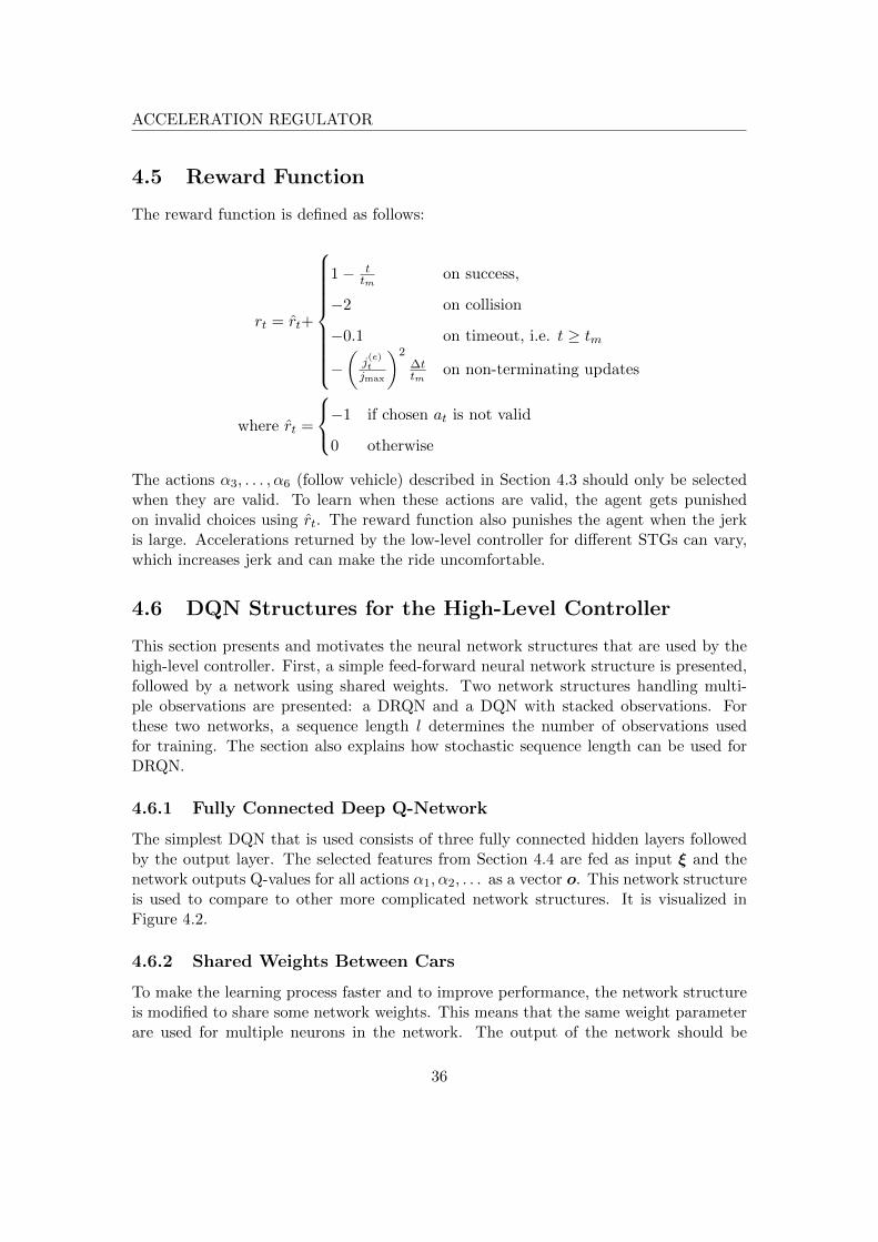
ACCELERATION REGULATOR
4.5 Reward Function
The reward function is defined as follows:
rt = rt+
1− ttm
on success,
−2 on collision
−0.1 on timeout, i.e. t ≥ tm
−(
j(e)tjmax
)2∆ttm
on non-terminating updates
where rt =
−1 if chosen at is not valid
0 otherwise
The actions α3, . . . , α6 (follow vehicle) described in Section 4.3 should only be selectedwhen they are valid. To learn when these actions are valid, the agent gets punishedon invalid choices using rt. The reward function also punishes the agent when the jerkis large. Accelerations returned by the low-level controller for different STGs can vary,which increases jerk and can make the ride uncomfortable.
4.6 DQN Structures for the High-Level Controller
This section presents and motivates the neural network structures that are used by thehigh-level controller. First, a simple feed-forward neural network structure is presented,followed by a network using shared weights. Two network structures handling multi-ple observations are presented: a DRQN and a DQN with stacked observations. Forthese two networks, a sequence length l determines the number of observations usedfor training. The section also explains how stochastic sequence length can be used forDRQN.
4.6.1 Fully Connected Deep Q-Network
The simplest DQN that is used consists of three fully connected hidden layers followedby the output layer. The selected features from Section 4.4 are fed as input ξ and thenetwork outputs Q-values for all actions α1, α2, . . . as a vector o. This network structureis used to compare to other more complicated network structures. It is visualized inFigure 4.2.
4.6.2 Shared Weights Between Cars
To make the learning process faster and to improve performance, the network structureis modified to share some network weights. This means that the same weight parameterare used for multiple neurons in the network. The output of the network should be
36
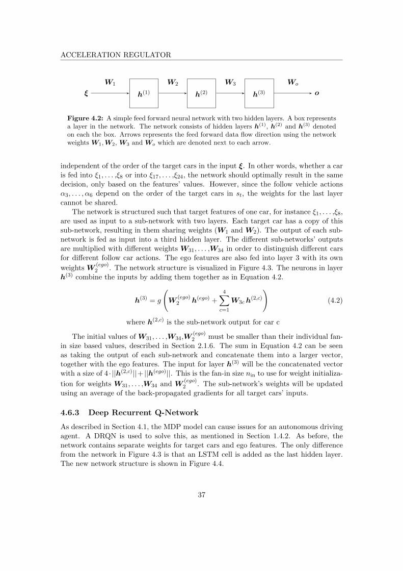
ACCELERATION REGULATOR
ξ h(1) h(2) h(3) o
W1 W2 W3 Wo
Figure 4.2: A simple feed forward neural network with two hidden layers. A box representsa layer in the network. The network consists of hidden layers h(1), h(2) and h(3) denotedon each the box. Arrows represents the feed forward data flow direction using the networkweights W1,W2, W3 and Wo which are denoted next to each arrow.
independent of the order of the target cars in the input ξ. In other words, whether a caris fed into ξ1, . . . ,ξ8 or into ξ17, . . . ,ξ24, the network should optimally result in the samedecision, only based on the features’ values. However, since the follow vehicle actionsα3, . . . , α6 depend on the order of the target cars in st, the weights for the last layercannot be shared.
The network is structured such that target features of one car, for instance ξ1, . . . ,ξ8,are used as input to a sub-network with two layers. Each target car has a copy of thissub-network, resulting in them sharing weights (W1 and W2). The output of each sub-network is fed as input into a third hidden layer. The different sub-networks’ outputsare multiplied with different weights W31, . . . ,W34 in order to distinguish different carsfor different follow car actions. The ego features are also fed into layer 3 with its own
weights W(ego)2 . The network structure is visualized in Figure 4.3. The neurons in layer
h(3) combine the inputs by adding them together as in Equation 4.2.
h(3) = g
(W
(ego)2 h(ego) +
4∑c=1
W3c h(2,c)
)(4.2)
where h(2,c) is the sub-network output for car c
The initial values of W31, . . . ,W34,W(ego)2 must be smaller than their individual fan-
in size based values, described in Section 2.1.6. The sum in Equation 4.2 can be seenas taking the output of each sub-network and concatenate them into a larger vector,together with the ego features. The input for layer h(3) will be the concatenated vectorwith a size of 4 · ||h(2,c)||+ ||h(ego)||. This is the fan-in size nin to use for weight initializa-
tion for weights W31, . . . ,W34 and W(ego)2 . The sub-network’s weights will be updated
using an average of the back-propagated gradients for all target cars’ inputs.
4.6.3 Deep Recurrent Q-Network
As described in Section 4.1, the MDP model can cause issues for an autonomous drivingagent. A DRQN is used to solve this, as mentioned in Section 1.4.2. As before, thenetwork contains separate weights for target cars and ego features. The only differencefrom the network in Figure 4.3 is that an LSTM cell is added as the last hidden layer.The new network structure is shown in Figure 4.4.
37
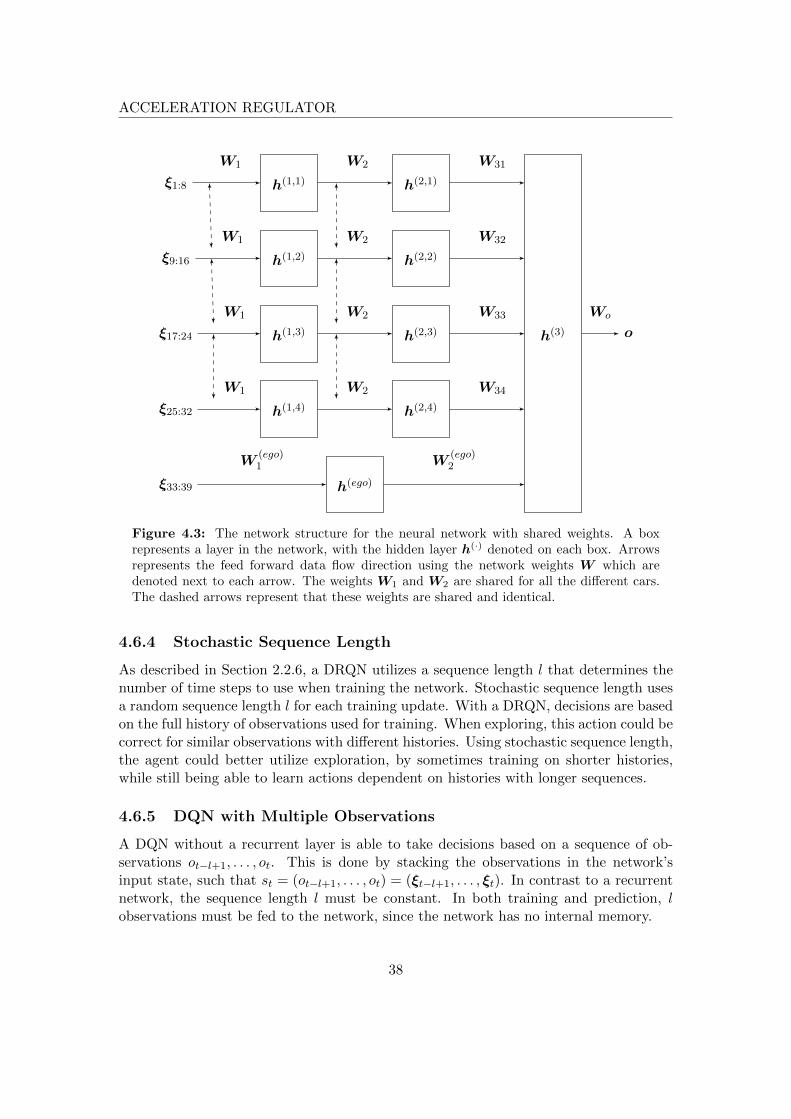
ACCELERATION REGULATOR
ξ1:8 h(1,1) h(2,1)
ξ9:16 h(1,2) h(2,2)
ξ17:24 h(1,3) h(2,3)
ξ25:32 h(1,4) h(2,4)
W1 W2 W31
W1 W2 W32
W1 W2 W33
W1 W2 W34
ξ33:39 h(ego)
W(ego)1 W
(ego)2
h(3) o
Wo
Figure 4.3: The network structure for the neural network with shared weights. A boxrepresents a layer in the network, with the hidden layer h(·) denoted on each box. Arrowsrepresents the feed forward data flow direction using the network weights W which aredenoted next to each arrow. The weights W1 and W2 are shared for all the different cars.The dashed arrows represent that these weights are shared and identical.
4.6.4 Stochastic Sequence Length
As described in Section 2.2.6, a DRQN utilizes a sequence length l that determines thenumber of time steps to use when training the network. Stochastic sequence length usesa random sequence length l for each training update. With a DRQN, decisions are basedon the full history of observations used for training. When exploring, this action could becorrect for similar observations with different histories. Using stochastic sequence length,the agent could better utilize exploration, by sometimes training on shorter histories,while still being able to learn actions dependent on histories with longer sequences.
4.6.5 DQN with Multiple Observations
A DQN without a recurrent layer is able to take decisions based on a sequence of ob-servations ot−l+1, . . . , ot. This is done by stacking the observations in the network’sinput state, such that st = (ot−l+1, . . . , ot) = (ξt−l+1, . . . , ξt). In contrast to a recurrentnetwork, the sequence length l must be constant. In both training and prediction, lobservations must be fed to the network, since the network has no internal memory.
38
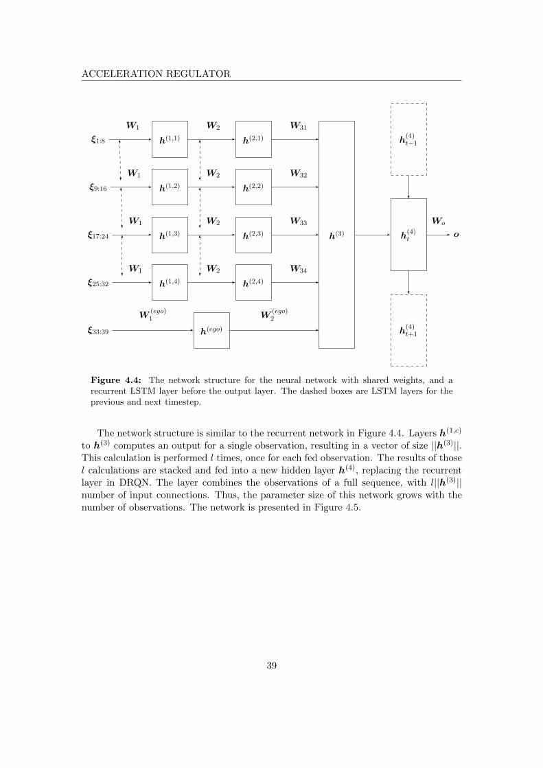
ACCELERATION REGULATOR
ξ1:8 h(1,1) h(2,1)
ξ9:16 h(1,2) h(2,2)
ξ17:24 h(1,3) h(2,3)
ξ25:32 h(1,4) h(2,4)
W1 W2 W31
W1 W2 W32
W1 W2 W33
W1 W2 W34
ξ33:39 h(ego)
W(ego)1 W
(ego)2
h(3)
h(4)t−1
h(4)t
h(4)t+1
o
Wo
Figure 4.4: The network structure for the neural network with shared weights, and arecurrent LSTM layer before the output layer. The dashed boxes are LSTM layers for theprevious and next timestep.
The network structure is similar to the recurrent network in Figure 4.4. Layers h(1,c)
to h(3) computes an output for a single observation, resulting in a vector of size ||h(3)||.This calculation is performed l times, once for each fed observation. The results of thosel calculations are stacked and fed into a new hidden layer h(4), replacing the recurrentlayer in DRQN. The layer combines the observations of a full sequence, with l||h(3)||number of input connections. Thus, the parameter size of this network grows with thenumber of observations. The network is presented in Figure 4.5.
39

ACCELERATION REGULATOR
h(3)t−l+1
. . .ξt−l+1
...
h(3)t−1
. . .ξt−1
h(3)t
. . .ξt
h(4)t
o
Wo
Figure 4.5: DQN stacked network structure, where l observations are used as input. Eachobservation is fed into a network with the same structure as the shared weights network
(Figure 4.3), but h(4)t is added before the output layer, which merges all l observations. The
horizontal dots is a shorthand for the entire shared weights structure.
40

5Result
This chapter presents the performance of the Acceleration Regulator when it is usedto comfortably drive a car, across multiple traffic crossings and with target cars withdifferent drivers’ behaviors, as described in Section 1.2 and 1.3. In Section 1.6, successrate was mentioned to be used for evaluation of the Acceleration Regulator. The firstsection in this chapter describes all the metrics used for evaluating the performance ofthe Acceleration Regulator. The next section presents the result for a simple crossingwith one car. Thereafter, shared weights between cars is compared to a standard fullyconnected feed forward network. The following section shows how well the agent isable to generalize between different scenarios. The last section presents how well theego agent can recognize other agents’ behaviors, by using several observations, and thusimprove the policy. The hyper-parameters used for each scenario, as well as more detailsabout target cars, which are not explicitly stated next to the results, can be found inAppendix A and Appendix B.
5.1 Evaluation Metrics
In traditional machine learning, the training progress can be evaluated by using the lossfunction. With a DQN, the policy can improve even if the training loss is increasing [10].For instance, predicting actions for unexplored states will typically increase loss, even ifprogression is made. Therefore, the training loss is not necessarily an indicator of thelearning progress and several other measurements are necessary.
Three metrics were selected for measurement of a training session: success rate,average episodic reward and collision to fail ratio. With these metrics, the distributionbetween the three terminating states can be analyzed. The success graph presents thesuccess to fail ratio averaged over the last 100 episodes. Both collisions and timeoutsare considered as failures. Average episodic reward is the summed reward over a wholeepisode, then averaged over 100 episodes. The collision to fail ratio displays the ratio
41
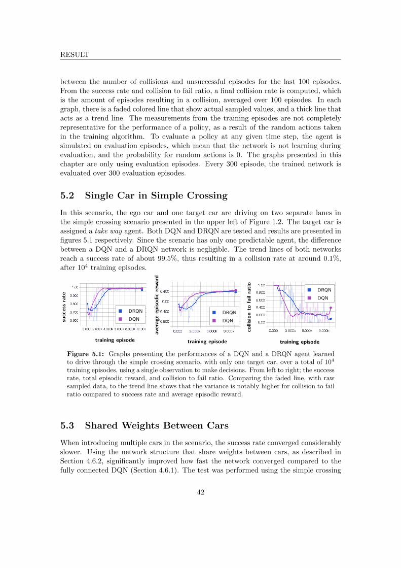
RESULT
between the number of collisions and unsuccessful episodes for the last 100 episodes.From the success rate and collision to fail ratio, a final collision rate is computed, whichis the amount of episodes resulting in a collision, averaged over 100 episodes. In eachgraph, there is a faded colored line that show actual sampled values, and a thick line thatacts as a trend line. The measurements from the training episodes are not completelyrepresentative for the performance of a policy, as a result of the random actions takenin the training algorithm. To evaluate a policy at any given time step, the agent issimulated on evaluation episodes, which mean that the network is not learning duringevaluation, and the probability for random actions is 0. The graphs presented in thischapter are only using evaluation episodes. Every 300 episode, the trained network isevaluated over 300 evaluation episodes.
5.2 Single Car in Simple Crossing
In this scenario, the ego car and one target car are driving on two separate lanes inthe simple crossing scenario presented in the upper left of Figure 1.2. The target car isassigned a take way agent. Both DQN and DRQN are tested and results are presented infigures 5.1 respectively. Since the scenario has only one predictable agent, the differencebetween a DQN and a DRQN network is negligible. The trend lines of both networksreach a success rate of about 99.5%, thus resulting in a collision rate at around 0.1%,after 104 training episodes.
successrate
DRQN
DQN
training episode
ave
rageep
isodic
reward
DRQN
DQN
training episode
collisionto
failratio
DRQN
DQN
training episode
Figure 5.1: Graphs presenting the performances of a DQN and a DRQN agent learnedto drive through the simple crossing scenario, with only one target car, over a total of 104
training episodes, using a single observation to make decisions. From left to right; the successrate, total episodic reward, and collision to fail ratio. Comparing the faded line, with rawsampled data, to the trend line shows that the variance is notably higher for collision to failratio compared to success rate and average episodic reward.
5.3 Shared Weights Between Cars
When introducing multiple cars in the scenario, the success rate converged considerablyslower. Using the network structure that share weights between cars, as described inSection 4.6.2, significantly improved how fast the network converged compared to thefully connected DQN (Section 4.6.1). The test was performed using the simple crossing
42

RESULT
scenario with a varied number of target cars, all using a take way agent. See Table B.1 inappendix for the complete list of scenarios. The success rate for the trend line convergesto 96% after 4 · 104 episodes for shared weights, which is better than 82% after 4 · 104
episodes for the fully connected neural network structure. The evaluation graphs forboth networks are shown in Figure 5.2. Note that the rewards are similar between bothnetworks, which means that there is room for improving the reward function.
successrate
Shared
Unshared
training episode
ave
rageep
isodic
reward
Shared
Unshared
training episode
collisionto
failratio
Shared
Unshared
training episode
Figure 5.2: The figure shows that the success rate for a network with shared weights(brown line) converge faster than the fully connected network structure which do not shareweights (turquoise line).
5.4 Generalize a Policy Across Different Scenarios
An agent is tested to learn on all crossing scenarios described in Section 1.4.1, to evaluatewhether the same agent can generalize its policy across multiple scenarios. The completelist of scenarios is given in Table B.2 in the appendix. A network starting to learnfrom random weights did not perform well on these scenarios. Therefore, a networkis first trained on only the simple crossing scenario with a varied number of cars for8 · 104 episodes. Once the network solves a simple crossing, the learning process is thenrestarted, with the same network, but trained on all crossing scenarios, and with anempty experience memory. The probability for taking random actions starts at 30%instead of 100% since the network is not initialized with random weights. The networkconverge to a success rate of about 95% after training on all crossing scenarios, for 5 ·104
episodes. The corresponding graphs for the result is presented if Figure 5.3.
successrate
training episode
ave
rageep
isodic
reward
training episode
collisionto
failratio
training episode
Figure 5.3: Graphs presenting the performance of a DRQN agent learned to drive throughthe all scenarios with 1 to 4 target cars.
43

RESULT
5.5 Recognizing Behavior
The following sections describe how the different network structures performed whenlearning different target car behaviors, while driving in the simple crossing from Figure1.2. Specifically, the results for DQNs with one or multiple observations, and DRQNswith different sequence lengths and observations used only for preparing the LSTM cell’sstate are shown. Table B.3 in the appendix lists the scenarios used for all tests in thefollowing sections.
5.5.1 Network with Recurrent Layer
There was a significant performance improvement in using a DRQN instead of a DQNwith a single observation. In other words, the environment for these scenarios is bettermodeled as a POMDP instead of an MDP, as described in Section 1.4.2, and the egoagent needs multiple observations in order to draw enough conclusions about other cars’behaviors. The trend lines for DRQN converges towards a success rate of around 97.2%and a 0.85% collision rate, compared to a success rate of 87.5% and a collision rate of1.75% for DQN. The graphs for these two networks are shown in Figure 5.4.
successrate
DRQN
DQN
training episode
ave
rageep
isodic
reward
DRQN
DQN
training episode
collisionto
failratio
DRQN
DQN
training episode
Figure 5.4: Graphs presenting the performance of a DRQN (dark blue) compared to aDQN with a single observation (turquoise), running on scenarios with cars that have differentbehaviors. When compared a DRQN succeeds in 3 out of 4 attempts, where a DQN fails.
5.5.2 DRQN or DQN with Multiple Observations
According to [12], a DQN with a stacked history of observations can perform as well as aDRQN, with an LSTM layer, in the aspect of Q-value accuracy [12]. The results supportthis statement. The DRQN was compared to the network described in Section 4.6.5,that uses a DQN with 4 stacked observations. Even though the policy’s performances areequal, the computational complexity of a DQN with stacked observations is higher, whichmakes a DRQN preferable. The lower computational complexity in LSTM is a resultof its internal memory, which lead to the network requiring only a single observation tocompute an output [12, 27]. The agents’ performances for the two networks are comparedin Figure 5.5.
44

RESULTsuccessrate
DRQN
DQN stacked
training episode
ave
rageep
isodic
reward
DRQN
DQN stacked
training episode
collisionto
failratio
DRQN
DQN stacked
training episode
Figure 5.5: The performances of a DRQN (blue) and a DQN with 4 stacked observations(green) are very similar, as suggested by Hausknecht and Stone’s theory.
5.5.3 Fixed or Stochastic Sequence Length
The DRQN network was run with different combinations of sequence lengths and numberof preparing observations (as described in Section 2.2.6). Figure 5.6 shows the differencebetween using a fixed sequence length l = 4, trained on the last single observation,compared to a stochastic sequence length between 1 and 4, also trained on the lastobservation. The results show that the trend lines for the success rate between thesetwo setups are negligible. From the trend lines, both networks converge to a success rateof 97.2%, resulting in a collision rate of about 0.85% for stochastic sequence length and0.95% for fixed sequence length.
successrate
Stochastic l
Fixed l = 4
training episode
ave
rageep
isodic
reward
Stochastic l
Fixed l = 4
training episode
collisionto
failratio
Stochastic l
Fixed l = 4
training episode
Figure 5.6: This is the result between DRQN using stochastic sequence length, randomizedbetween 1 and 4 at each training step, compared to a fixed sequence length of 4. In bothcases, only one observation was trained on.
The performance of having observations to build the LSTM’s cell state before trainingwas also measured. Given a sequence length of 4, where the algorithm uses observations(o1, o2, o3, o4), the DRQN in the last paragraph trains only on o4, and o1, o2, o3 are usedto prepare the cell state. Another network was trained using a sequence length of 4,training on all 4 observations instead of only the last one. This makes the initial LSTMstate zero in every training update. As can be seen in Figure 5.7, this network performedworse compared to the DRQN training on only the last observation.
The results show that the best performing network for the scenarios with multiplebehaviors is a DRQN training only on the last observation. The learning algorithm useda stochastic sequence length and got a success rate of 97.2% and collision rate of 0.85%.Even if DQN with stacked observations achieved about the same performance, the DRQN
45
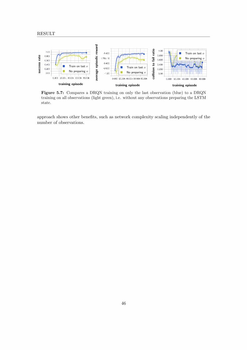
RESULTsuccessrate
Train on last o
No preparing o
training episode
ave
rageep
isodic
reward
Train on last o
No preparing o
training episode
collisionto
failratio
Train on last o
No preparing o
training episode
Figure 5.7: Compares a DRQN training on only the last observation (blue) to a DRQNtraining on all observations (light green), i.e. without any observations preparing the LSTMstate.
approach shows other benefits, such as network complexity scaling independently of thenumber of observations.
46

6Discussion
The results show a success rate of around 97.2% for recognizing behaviors, and 95%when driving in all four crossings. However, the ego car still collides too often. The egocar is limited to drive comfortably, meaning that in some cases, the ego agent is notallowed to break hard enough. In a complete system, a collision avoidance procedure,which does not have comfortability constraints, would need to take over the control toensure a safe ride. However, the probability of this to happen must be much lower, whichindicates the need for further improvements to be made before deployment. Even if thecollision avoidance systems can take care of emergency situations, the policy learned byreinforcement learning should not have knowledge of these. The policy’s goal should beto plan a safe and comfortable trajectory, without having the option to rely on emergencysystems.
The choice of scenarios used for training the agent greatly influence the learnedpolicy. For example, during testing, the ego agent sometimes did not learn to accelerateafter it had stopped before a crossing. A possible explanation could be that the agenttypically timed other cars very well, and thus rarely ended up in a situation where ithad to fully stop before the crossing. It would not learn how to continue from that state,simply because it was rare for the agent to visit that state. In order to test if this wasthe case, a new configuration to the same scenario was added, where the ego car startedin this state; standing still at the crossing. This increased the distribution of such states,and the agent successfully learned how to continue from a state where the ego car isstanding still in front of the crossing.
Since the environment in this project is built for reinforcement learning in mind, itmight be biased in its construction, and this could be a problem. Whenever a targetcar reaches the end of its lane, it is immediately put at the start of its lane. This caris considered a new car, since the old one left the observable area for the ego car, anda new car entered the observable area at the start of the lane. This might be one suchbiased artifact, and could cause unwanted artifacts to the learning algorithm, as the
47

DISCUSSION
policy might exploit that new cars always appear when old ones disappear.Running reinforcement learning for autonomous driving in a simulator is very fast
and cost effective, compared to real traffic. However, in real traffic, where sensors arenot ideal, cars might pop up, or disappear anywhere, while our trained agent learns thatnew vehicles only pop up at the start of the lane. This could possibly have been avoidedby, for instance, stochastically spawning cars or adding noise to the input in the trafficsimulator. Continuing, actual human behavior probably differ from the programmedbehaviors added to the simulator. It might even be so, that the wanted behavior of thoseagents could be the policy that the ego agent is trying to learn. The difference betweenthe simulator and real world traffic should therefore be minimized, for deployment inreal traffic.
Reducing the action space for the high-level controller by choosing discrete actionscould be an advantage, as described in Chapter 4. Though, actions that can be performedby the ego agent are limited by how the actions are implemented. To include morefreedom, more actions with different strengths must be added. Also, the ego agent oftenlearned to quickly switch between the two actions take way and give way, for keepinga constant acceleration. This introduces jerk. A policy gradient or actor-critic methodcould instead control the acceleration directly, and therefore have more control over thevehicle.
Initially, the Acceleration Regulator consisted of a high-level only choosing betweentwo discrete actions, which either increased or decreased the ego car’s acceleration lin-early, instead of using the implemented STGs. This led to high jerk. A zero-jerk actionwas therefore introduced, used to maintain the current acceleration. By including thisaction, however, the agent did not learn how to drive. The reason for this is unclear,and further testing is needed to make a conclusion.
The definition of the reward function plays a large role in what agents attempt tolearn. However, the policy is typically not improved by tuning the reward function, asit only tells what goal the agent should achieve. For example; the reward function usedin this thesis project attempts to solve the solution as fast as possible. An alternativesolution is to punish inactivity, by punishing low velocities. This reward function teachesthe agent that it is good to never stop. It will be good at timing the gaps between cars,but when there is no gap, it would rather collide than stop in front of the crossing. Ifthe agent does not learn, or learns to solve the wrong problem, as in the example, thenadjusting the reward function is correct.
When learning on multiple traffic crossings (Section 5.4), a network with randominitial weights did not learn how to drive. However, when the agent was initiated withan already learned, simpler policy, the agent could improve to actually learn the moredifficult problem. To not start from zero, but to take advantage of an already learnedpolicy, is a good idea. This leads to another technique called imitation learning [8],where a policy is initiated by copying parts of another agent’s behavior before startingthe reinforcement learning loop.
48

DISCUSSION
6.1 Future Work
To be able to apply this solution in traffic, the agent must be able to control the lateralposition. There might be situations where the agent need to position the car at any sideof the lane in order to drive around other vehicles or to better take advantage of gaps.Also, the proposed solution could be extended to work on other areas than crossings.One such area could be to learn how to use both longitudinal and lateral control in orderto change from one lane to another.
To make reinforcement learning safer, Shalev-Shwartz et al. propose a method ofdecreasing the (negative) reward r for an accident if the probability p of that accidenthappening is low, such that r < −1
p [8]. The expected reward can otherwise becomeinsignificant on very unlikely accidents. The solution, however, introduces high variance.Another method suggested by Lipton et al., called intrinsic fear, is to let a second neuralnetwork learn how dangerous a state s ∈ S is. That network can be used to avoid endingup in dangerous situations by making the agent fear them. The learning algorithm thendoes not only maximize reward, it also minimizes the danger level of a state [40].
In this thesis, features used in the state were manually selected. The learning algo-rithm used, DRQN, can also make use of lower level of observation data, such as rawsampled data points of the road. A solution using such features could eliminate manualfeature selection. A technique applicable when using lower level features, presented in[37], is to force the agent to learn specific selected high level features, needed to takecorrect actions during training, such as known traffic rules. The agent is guided to learnand identify this information, which can improve performance [37].
49

7Conclusion
In this thesis, Deep Q-Learning has been implemented in the domain of autonomousvehicle control. The goal of the ego agent is to drive through different crossings, byadjusting longitudinal acceleration using STGs. High-level features computed from acoordinate system are used as observations in order to achieve this. These features weredivided into target car features, fed once for each target car, and ego features, dependentonly on the ego car. Convergence of the neural network was shown to be improved bysharing weights between the first layers to which the target car features are fed, comparedto a fully connected neural network structure.
The results also show that trained policies can generalize over different types of trafficcrossings and driver behaviors. The same learned policy is able to respond to target cars’actions and handle traffic scenarios with a varied number of cars and different types ofcrossings, without knowing traffic rules or the type of crossing it drives in. Multipleobservations are needed in order to recognize cars’ behaviors, and can be utilized by forinstance a DRQN. A DQN with stacked observations is considered to have comparableperformance, but it requires a fixed sequence length and more parameters than theDRQN. A stochastic sequence length for DRQN was compared to a fixed sequence length.However, results indicate similar performance between the two.
The results are still limited to the tested traffic scenarios and driver behaviors, andexpanding the domain beyond a simulator is a natural next step. The selected featuresare also limited to crossings. Utilization of lower level data could extend the solutionbeyond crossings without further handcrafting of additional features.
50

Bibliography
[1] NHTSA, “Distracted driving 2013,” NHTSA’s National Center for Statistics andAnalysis, 2015.
[2] M. Distner, M. Bengtsson, T. Broberg, and L. Jakobsson, “City safety—a systemaddressing rear-end collisions at low speeds,” in Proc. 21st International TechnicalConference on the Enhanced Safety of Vehicles, no. 09-0371, 2009.
[3] W. Kabbaj, “What a driverless world could look like,” TED@UPS Atlanta, 2016.
[4] Google, “Google self-driving car project, on the road,” https://www.google.com/selfdrivingcar/where/, 2016, accessed: 2016-11-25.
[5] DARPA,“Darpa urban challenge,” http://archive.darpa.mil/grandchallenge/, 2007,accessed: 2017-06-26.
[6] A. Krizhevsky, I. Sutskever, and G. E. Hinton, “Imagenet classification with deepconvolutional neural networks,” in Advances in neural information processing sys-tems, 2012, pp. 1097–1105.
[7] D. Silver, A. Huang, C. J. Maddison, A. Guez, L. Sifre, G. Van Den Driessche,J. Schrittwieser, I. Antonoglou, V. Panneershelvam, M. Lanctot et al., “Masteringthe game of go with deep neural networks and tree search,” Nature, vol. 529, no.7587, pp. 484–489, 2016.
[8] S. Shalev-Shwartz, S. Shammah, and A. Shashua, “Safe, multi-agent, reinforcementlearning for autonomous driving,” CoRR, vol. abs/1610.03295, 2016.
[9] M. Bojarski, D. Del Testa, D. Dworakowski, B. Firner, B. Flepp, P. Goyal, L. D.Jackel, M. Monfort, U. Muller, J. Zhang et al., “End to end learning for self-drivingcars,” arXiv preprint arXiv:1604.07316, 2016.
[10] V. Mnih, K. Kavukcuoglu, D. Silver, A. Graves, I. Antonoglou, D. Wierstra, andM. Riedmiller, “Playing atari with deep reinforcement learning,” arXiv preprintarXiv:1312.5602, 2013.
51

BIBLIOGRAPHY
[11] T. P. Lillicrap, J. J. Hunt, A. Pritzel, N. Heess, T. Erez, Y. Tassa, D. Silver, andD. Wierstra, “Continuous control with deep reinforcement learning,” CoRR, vol.abs/1509.02971, 2015. [Online]. Available: http://arxiv.org/abs/1509.02971
[12] M. Hausknecht and P. Stone, “Deep recurrent q-learning for partially observablemdps,” arXiv preprint arXiv:1507.06527, 2015.
[13] I. D. Jacobson, L. G. Richards, and A. R. Kuhlthau, “Models of human com-fort in vehicle environments,” HUMAN FACTORS IN TRANSPORT RESEARCHEDITED BY DJ OBORNE, JA LEVIS, vol. 2, 1980.
[14] S. Shalev-Shwartz, N. Ben-Zrihem, A. Cohen, and A. Shashua, “Long-term planningby short-term prediction,” arXiv preprint arXiv:1602.01580, 2016.
[15] Z. C. Lipton, J. Gao, L. Li, J. Chen, and L. Deng, “Combating reinforcementlearning’s sisyphean curse with intrinsic fear,” arXiv preprint arXiv:1611.01211,2017.
[16] M. Wahde, Biologically inspired optimization methods: an introduction. WIT press,2008.
[17] W. S. McCulloch and W. Pitts, “A logical calculus of the ideas immanent in nervousactivity,” Bulletin of Mathematical Biology, vol. 5, pp. 115–133, 1943, classics ofTheoretical Biology.
[18] I. Goodfellow, Y. Bengio, and A. Courville, Deep Learning. MIT Press, 2016,http://www.deeplearningbook.org.
[19] K. Hornik, “Approximation capabilities of multilayer feedforward networks,” Neuralnetworks, vol. 4, no. 2, pp. 251–257, 1991.
[20] S. Ruder, “An overview of gradient descent optimization algorithms,” CoRR, vol.abs/1609.04747, 2016.
[21] M. A. Nielsen, “Neural networks and deep learning,” Determination Press, 2015.
[22] C. M. Bishop, “Pattern recognition,” Machine Learning, vol. 128, pp. 1–58, 2006.
[23] J. Sjoberg and L. Ljung, “Overtraining, regularization and searching for a minimum,with application to neural networks,” International Journal of Control, vol. 62, no. 6,pp. 1391–1407, 1995.
[24] X. Glorot and Y. Bengio, “Understanding the difficulty of training deep feedforwardneural networks.” in Aistats, vol. 9, 2010, pp. 249–256.
[25] P. J. Werbos, “Backpropagation through time: what it does and how to do it,”Proceedings of the IEEE, vol. 78, no. 10, pp. 1550–1560, 1990.
52

BIBLIOGRAPHY
[26] R. J. Williams and D. Zipser, “A learning algorithm for continually running fullyrecurrent neural networks,” Neural computation, vol. 1, no. 2, pp. 270–280, 1989.
[27] S. Hochreiter and J. Schmidhuber, “Long short-term memory,” Neural computation,vol. 9, no. 8, pp. 1735–1780, 1997.
[28] G. E. Hinton, N. Srivastava, A. Krizhevsky, I. Sutskever, and R. R. Salakhutdinov,“Improving neural networks by preventing co-adaptation of feature detectors,” arXivpreprint arXiv:1207.0580, 2012.
[29] N. Srivastava, G. E. Hinton, A. Krizhevsky, I. Sutskever, and R. Salakhutdinov,“Dropout: a simple way to prevent neural networks from overfitting.” Journal ofMachine Learning Research, vol. 15, no. 1, pp. 1929–1958, 2014.
[30] S. Bhatnagar, D. Precup, D. Silver, R. S. Sutton, H. R. Maei, and C. Szepesvari,“Convergent temporal-difference learning with arbitrary smooth function approxi-mation,” in Advances in Neural Information Processing Systems, 2009, pp. 1204–1212.
[31] L. P. Kaelbling, M. L. Littman, and A. W. Moore, “Reinforcement learning: Asurvey,” Journal of Artificial Intelligence Research, vol. 4, pp. 237–285, 1996.
[32] R. S. Sutton and A. G. Barto, Reinforcement learning: An introduction. MIT pressCambridge, 1998, vol. 1, no. 1.
[33] H. V. Hasselt, A. Guez, M. Hessel, and D. Silver, “Learning functions across manyorders of magnitudes,” CoRR, vol. abs/1602.07714, 2016.
[34] J. N. Tsitsiklis, B. Van Roy et al., “An analysis of temporal-difference learning withfunction approximation,” IEEE transactions on automatic control, vol. 42, no. 5,pp. 674–690, 1997.
[35] L.-J. Lin, “Self-improving reactive agents based on reinforcement learning, planningand teaching,” Machine learning, vol. 8, no. 3-4, pp. 293–321, 1992.
[36] V. Mnih, K. Kavukcuoglu, D. Silver, A. A. Rusu, J. Veness, M. G. Bellemare,A. Graves, M. Riedmiller, A. K. Fidjeland, G. Ostrovski et al., “Human-level controlthrough deep reinforcement learning,” Nature, vol. 518, no. 7540, pp. 529–533, 2015.
[37] G. Lample and D. S. Chaplot, “Playing FPS games with deep reinforcement learn-ing,” CoRR, vol. abs/1609.05521, 2016.
[38] R. S. Sutton, D. A. McAllester, S. P. Singh, Y. Mansour et al., “Policy gradientmethods for reinforcement learning with function approximation.” in NIPS, vol. 99,1999, pp. 1057–1063.
[39] V. R. Konda and J. N. Tsitsiklis, “Actor-critic algorithms.” in NIPS, vol. 13, 1999,pp. 1008–1014.
53

BIBLIOGRAPHY
[40] Z. C. Lipton, A. Kumar, J. Gao, L. Li, and L. Deng, “Combating deep rein-forcement learning’s sisyphean curse with reinforcement learning,” arXiv preprintarXiv:1611.01211, 2016.
54

Appendices
55

AHyper parameters
This appendix states the hyper parameters used during training. The parameters pre-sented in table A.1 are the default parameters, used for all training sessions presentedin the Result chapter, unless where other values are specified. Figure A.1 presents thenumber of neurons existing in each layer of the DRQN and DQN network. Figure A.2shows the number of neurons used in the tested fully connected network that does notcontain shared weights. When the experience memory is full, a random experience isreplaced with the new experience.
56

HYPER PARAMETERS
Name Notation Value
Exploration ε max(
0.1, eln(0.5)i2000
); where i is the episode counter
Discount Factor γ 0.99
Car Size s(c) [2,4]T
Max Lateral Acceleration alat 1.5
Distance to Intersection dmargin 1
Distance to Front Car doffset 6
Sight Range pmax 50
Max Speed vmax 30
Max Acceleration amax 5
Max Jerk jmax 3
Learning Rate η 10−3
Batch Size B 64
Update Interval ∆t 100030
Experience Memory Size N 106
Dropout Probability p 0.75
Sequence Length l l ∼ U [1,4]; l ∈ N; Randomized each update.
Build LSTM state h l − 1
Target Network Parameter τ 0.99
Table A.1: Default values used for simulation in the scenarios presented in the Resultchapter.
57

HYPER PARAMETERS
ξ1:8 32 16
ξ9:16 32 16
ξ17:24 32 16
ξ25:32 32 16
ξ33:39 16
64
32
32
32
o
Figure A.1: The number of neurons used at each layer of the network. The last layer isthe LSTM layer with 32 neurons. The same neuron count was used in all tests presentedin the Result chapter, except the fully connected network, which used an entierly differentstructure, presented in Figure A.2.
58

HYPER PARAMETERS
ξ 144 80 64 o
32
32
32
Figure A.2: The number of neurons used at each layer in the fully connected network.The last layer with 32 neurons is an LSTM layer.
59

BScenarios
This appendix chapter describes the scenarios that the agent is trained on. Each scenariois presented in Figure 1.2.
All scenarios used for testing generalization over multiple crossings are listed in tableB.2. The target cars in these scenarios are assigned a take way agent. A subset of thesescenarios, are used when comparing the performance of the shared network structure tothe fully connected network structure. These scenarios is presented in table B.1. Allscenarios used for testing generalization over multiple behaviors are listed in table B.3.
Crossing Cars Description
Simple Crossing 1
Simple Crossing 1 Ego car starts still at crossing.
Simple Crossing 2
Simple Crossing 2 Ego car must stop for crossing cars.
Simple Crossing 3
Simple Crossing 3 Ego car must stop for crossing cars.
Simple Crossing 4
Simple Crossing 4 Ego car must stop for crossing cars.
Simple Crossing 4 Ego car starts still at crossing.
Table B.1: Scenarios used when comparing shared network structure to a fully connectednetwork structure.
60
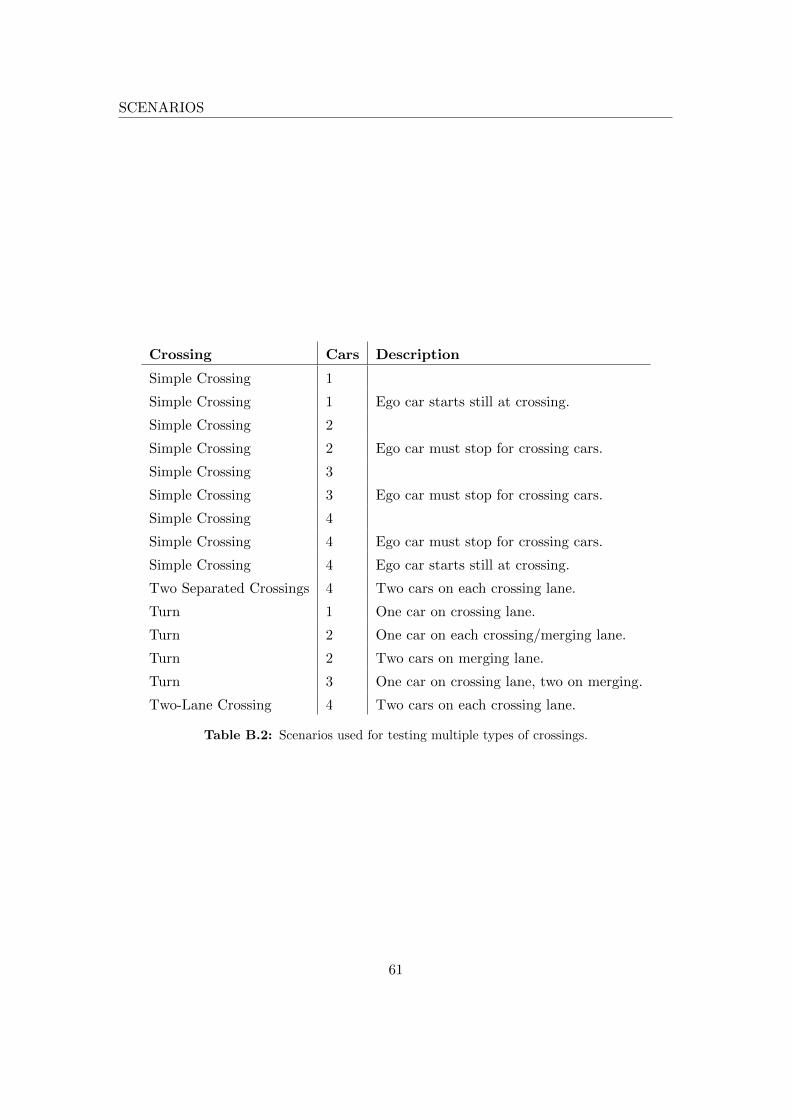
SCENARIOS
Crossing Cars Description
Simple Crossing 1
Simple Crossing 1 Ego car starts still at crossing.
Simple Crossing 2
Simple Crossing 2 Ego car must stop for crossing cars.
Simple Crossing 3
Simple Crossing 3 Ego car must stop for crossing cars.
Simple Crossing 4
Simple Crossing 4 Ego car must stop for crossing cars.
Simple Crossing 4 Ego car starts still at crossing.
Two Separated Crossings 4 Two cars on each crossing lane.
Turn 1 One car on crossing lane.
Turn 2 One car on each crossing/merging lane.
Turn 2 Two cars on merging lane.
Turn 3 One car on crossing lane, two on merging.
Two-Lane Crossing 4 Two cars on each crossing lane.
Table B.2: Scenarios used for testing multiple types of crossings.
61
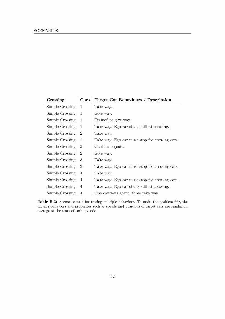
SCENARIOS
Crossing Cars Target Car Behaviours / Description
Simple Crossing 1 Take way.
Simple Crossing 1 Give way.
Simple Crossing 1 Trained to give way.
Simple Crossing 1 Take way. Ego car starts still at crossing.
Simple Crossing 2 Take way.
Simple Crossing 2 Take way. Ego car must stop for crossing cars.
Simple Crossing 2 Cautious agents.
Simple Crossing 2 Give way.
Simple Crossing 3 Take way.
Simple Crossing 3 Take way. Ego car must stop for crossing cars.
Simple Crossing 4 Take way.
Simple Crossing 4 Take way. Ego car must stop for crossing cars.
Simple Crossing 4 Take way. Ego car starts still at crossing.
Simple Crossing 4 One cautious agent, three take way.
Table B.3: Scenarios used for testing multiple behaviors. To make the problem fair, thedriving behaviors and properties such as speeds and positions of target cars are similar onaverage at the start of each episode.
62