automotive underbody flow study allen lewis …
TRANSCRIPT

AUTOMOTIVE UNDERBODY FLOW STUDY
by
ALLEN LEWIS WATSON, B.S.M.E.
A THESIS
IN
MECHANICAL ENGINEERING
Submitted to the Graduate Faculty of Texas Tech University in
Partial Fulfillment of the Requirements for
the Degree of
MASTER OF SCIENCE
IN
MECHANICAL ENGINEERING
Approved
Accepted
May, 1993

ACKNOWLEDGEMENTS
I would like to recognize the faculty and staff of the Texas Tech University
Department of Mechanical Engineering for their contributions of time and effort to this
thesis. I would also like to thank Dr. Oler and the members of my committee for their
efforts which made this thesis possible and my family and fellow students for their
support.
11

TABLE OF CONTENTS
A C K N 0 W LED G ME NT S ........................................................................... ii.
LIST OF FIGURES ................................................................................. v
LIST OF SYMBOLS AND ABBREVIATIONS ................................................ vii
CHAPTER
1. ~OD UcriON ....................................................................... 1
2. BACKGROU'ND ........................................................................ 2
2.1 Introduction .................................................................... 2
2.2 Literature Review .............................................................. 5
2.3 Basic Equations ............................................................... 14
2.4 Underbody Pressure Recovery Model ..................................... 15
3. NUMERICAL ANALYSIS OF FORD TAURUS AND F150 WIND TIJNNE.L DATA ........................................................................ 19
3.1 Analysis Procedure ........................................................... 19
3. 2 Taurus ......................................................................... . 20
3.3 F150 ............................................................................ 29
3.4 Summary ...................................................................... 43
4. EXPERIMENTAL APPARATUS AND TEST PROCEDURE ................... 44
4.1 Wind Tunnel Test Facility ................................................... 44
4.2 Ex~rimental Model .......................................................... 46
4.3 Instrumentation ............................................................... 49
4.4 Experimental Procedure ...................................................... 52
5. DISCUSSION OF EXPERIMENTAL RESULTS ................................ . 55
5.1 Introduction ................................................................... 55
5.2 Anemometer Results ......................................................... 55
w

5.3 Engine Bay Pressure Measurements ....................................... 60
5.4 Underbody Pressure Results ................................................ 64
5.5 Summary ...................................................................... 67
6. CONCLUSIONS AND RECOMMENDATIONS .................................. 72
6.1 Conclusions ................................................................... 72
6.2 Recommendations ............................................................ 73
REFERENCES ...................................................................................... 7 4
. IV
LIST OF FIGURES
2.1 ~_COOL Air Path ......................................................................... 4
2 2 c te r Pr D. ·b · '" T s· f Ai D 6 . en r me essure lStn uuons 10r wo tzes o r ams .......................... .
2. 3 Comparison of Ground plane and Underbody Pressures ................................. 7
2.4 Velocity Distribution Underneath a Car ..................................................... 9
2.5 Engine Compartment and Groundplane Pressures for Two Dam Sizes ................ 10
2.6 Flow Field Effects of Front Underbody Dams ........................................... .11
2. 7 Schematic Diagram of Air Path Through the Cooling System .......................... 13
2. 8 Generalized View of Engine and Underbody Flow Region ............................. 16
2. 9 Graphical Depiction of Underbody Correlation ........................................... 18
3.1 Typical Taurus Plot of Underbody Pressure Coefficient Versus Radiator Velocity Ratio Squared ....................................................................... 21
3.2 Plot of Underbody Pressure Coefficient Versus Radiator Velocity Ratio Squared for all Taurus Data Sets Combined ......................................................... 23
3.3 Plot of Underbody Pressure Coefficient Versus Radiator Velocity Ratio Squared for Taurus Data Sets with Combined Openings ........................................... 24
3.4 Plot of Underbody Pressure Coefficient Versus Radiator Velocity Ratio Squared for Taurus Data Sets with Isolated Openings .............................................. 25
3.5 Plot of Underbody Pressure Coefficient Versus Radiator Velocity Ratio Squared for Taurus Data Sets with Small Air Dams ................................................ 26
3.6 Plot of Underbody Pressure Coefficient Versus Radiator Velocity Ratio Squared for Taurus Data Sets with Large Air Dams ................................................ 27
3. 7 Common Slope Plot of Underbody Pressure Coefficient Versus Radiator Velocity Ratio Squared for Taurus Data Sets with Small and Large Air Dams ........ 28
3. 8 Typical Plot of Underbody Pressure Coefficient Versus Radiator Velocity Ratio Squared for the F150 ......................................................................... 30
3.9 Plot of Underbody Pressure Coefficient Versus Radiator Velocity Ratio Squared for all F150 Data Sets Combined ........................................................... 31
3.10 Plot of Underbody Pressure Coefficient Versus Radiator Velocity Ratio Squared for F 150 Data Sets with Large Spoilers .................................................... 32
3.11 Plot of Underbody Pressure Coefficient Versus Radiator Velocity Ratio Squared for F 150 Data Sets with Small Spoilers ................................................... .33
v

3.12 Same Slope Plot of Underbody Pressure Coefficient Versus Radiator Velocity Ratio Squared for F150 Data Sets with Large and Small Spoilers ...................... 34
3.13 Plot of Underbody Pressure Coefficient Versus Radiator Velocity Ratio Squared for Fl50 Data Sets with Large, Small, and No Spoilers ................................. 35
3.14 Plot of Underbody Pressure Coefficient Versus Radiator Velocity Ratio Squared for F150 Data Sets with 105 in. squared Openings ...................................... 37
3.15 Plot of Underbody Pressure Coefficient Versus Radiator Velocity Ratio Squared for Fl50 Data Sets with 210 in. squared Openings ...................................... 38
3.16 Plot of Underbody Pressure Coefficient Versus Radiator Velocity Ratio Squared for Fl50 Data Sets with 315 in. squared Openings ...................................... 39
3.17 Plot of Underbody Pressure Coefficient Versus Radiator Velocity Ratio Squared for Fl50 Data Sets with 420 in. squared Openings ...................................... 40
3.18 Plot of Underbody Pressure Coefficient Versus Radiator Velocity Ratio Squared for F150 Data Sets with 525 in. squared Openings ...................................... 41
3.19 Plot of Underbody Pressure Coefficient Versus Radiator Velocity Ratio Squared for F150 Data Sets with Small and Large Air Dams ..................................... .42
4.1 Schematic of Texas Tech Wind Tunnel .................................................... 45
4. 2 Experimental Model .......................................................................... 48
4.3 Instrumentation Schematic ................................................................... 51
5.1 Average Underbody Velocity Versus Average Internal Velocity ........................ 56
5.2 Ratio of Internal Flow Rate to Underbody Flow Rate Versus Average Internal Velocity ........................................................................................ 59
5.3 Ratio of Internal Flow Rate to Underbody Flow Rate Versus Ratio of Average Internal Velocity to Freestream Velocity ................................................... 61
5.4 Engine Bay Pressure Coefficient Versus Radiator Velocity Ratio Squared ............ 62
5. 5 Engine Bay Pressure Coefficient Versus Limited Radiator Velocity Ratio Squared ........................................................................................ 63
5. 6 Underbody Pressure Coefficient Distribution for Freestream Velocity of 41.76 ftls ...................................................................................... 65
5. 7 Underbody Pressure Coefficient Distribution for Freestream Velocity of 49.40 ftls ...................................................................................... 68
5. 8 Underbody Pressure Coefficient Distribution for Freestream Velocity of 59.84 ftls ...................................................................................... 69
5. 9 Generalized Depiction of Underbody Pressure Coefficient Distributions for the Three Flow Regimes ......................................................................... 70
. Vl

CHAPTER!
INTRODUCTION
The underbody flow field characteristics of a vehicle are functions of vehicle
geometry, external flow conditions, and the engine bay flow patterns. A more thorough
knowledge of the nature of this flow field would aid those who seek to design more
efficient and effective engine cooling systems. A correlation that describes the pressure
changes across the engine bay and underbody of a vehicle will be introduced in Chapter 2.
One component of this study involved numerically analyzing wind tunnel data for a
full-size Ford Taurus Sedan and a Ford Fl50 truck in order to test the validity of the
correlation. The data was grouped according to parameters such as air dam size, frontal
opening area, and opening arrangement in order to evaluate the correlation under a variety
of conditions.
The second aspect of the investigation dealt with running wind tunnel tests on a
generically shaped 0.2-scale model of an automotive front end. These tests were
performed to evaluate the conclusions reached in the previous numerical analysis. Another
purpose of the tests was to examine the interaction process between the external and
internal flows in the underbody region.
1

CHAPTER2
BACKGROUND
2.1 Introduction
Automotive cooling systems have in the past been developed via a relatively non
analytical procedure which led to oversized and inefficient cooling configurations. The
recent emphasis placed on improving vehicle aerodynamics has made this practice a costly
one since the cooling process accounts for a substantial portion of the drag. According to
Hucho, poorly designed cooling systems can increase drag by up to 10 percent whereas
efficiently designed configurations can limit this increase to only 2 percent [1]. Another
consideration is that inefficient cooling systems may eventually require modification which
could create costly delays in bringing a new vehicle to the marketplace. Therefore, an
analytical method of designing the cooling system based on experimental tests would have
great value in improving overall vehicle performance and reducing production expenses.
The interaction of the external and internal flow fields for a vehicle determines to a
great extent its cooling performance. There are two locations where these flow interactions
take place. The frrst position is at the frontal openings such as the grille, chin, bumper, and
bottom intakes where the ram air flow enters. The second location is at the bottom of the
vehicle behind the air dam where the cooling flow exits from the engine bay and interacts
with the freestream generated underbody flow. The engine bay underbody openings can be
located in front of or behind the front axle depending on the exact placement of the engine
and transaxle. This research effort focuses on the internal and external flow interactions
which take place in the engine bay and underbody region.
The overall objective of this project is to investigate the nature of the automotive
underbody flow field. As mentioned previously, the interaction of the external underbody
flow with the internal engine bay flow is the primary phenomena of interest Previous
2

studies have examined the internal and external flow interactions which occur at the frontal
openings. For this study, the internal flow is followed from the exit of the radiator fan
through the engine bay to the underbody. It is hoped that this study will aid in the
development of a suitable physical model of the flow interaction process in the underbody
region.
This model can then be incorporated into the computer program TIU_COOL which
is being developed at Texas Tech University with the support of the Ford Motor Company.
ITU_COOL is a program with the primary purpose of predicting the underhood air flow
rate and the secondary purpose of calculating the fluid and thermal properties between the
major underhood components shown in Figure 2.1 [2]. An automotive engineer can make
use of the program as a design tool to test the efficiency and effectiveness of various
cooling system configurations. The physical models used by TIU_COOL to calculate
these quantities have been verified with experimental wind tunnel data for a full-size Ford
Taurus Sedan and an F150 pickup truck.
However, the program does not accurately model the underbody flow interaction
because previously there was relatively little experimental data to support such a physical
representation. TIU _COOL instead determines, for computational convenience, the
underbody pressure recovery by using the following correlation,
(2.1)
In Equation 2.1, K" is an empirically defined underbody pressure recovery coefficient [2].
Values for K" were calculated using experimental wind tunnel data for the Taurus and
F150. Station 9 represents the conditions at the engine bay exit while Station 0 refers to the
overall ambient conditions surrounding the vehicle.
In contrast, Station 10 does not represent a specific underbody location and the
pressure at that point is arbitrarily defmed as equal to the ambient pressure. The other
3

~ - .. - --
v Grille
Bypass Region
-----
---Condenser
• Shroud Region
--
- --
Radiator Fan
Figure 2.1 TTIJ _COOL Air Path [2]
4
1 - - --.... - --h
Engine Underbod y Bay

properties at Station 10 are unknown and undefined [2]. Therefore, the physical
modelling of the underhood flow process ceases at the engine bay exit.
2.2 Literature Review
Relatively little research effort has been directed towards the actual modelling of the
interaction of the cooling air flow with the underbody flow field. There have been,
however, extensive studies performed on other aspects of this phenomena.
Schenkel performed wind tunnel studies on a 0.37 5 scale model of a notchback
sedan which revealed that the underbody pressure levels vary widely depending on the
horizontal location beneath the vehicle centerline (Figure 2.2) [3]. From the front bumper
to the front axle, the pressure levels were generally higher than ambient conditions.
Schenkel notes that this distribution results from the deceleration of the freestream flow as
it comes in contact with the bumper, front axle, and other protrusions [3].
However, once the flow passed the front axle the distribution fell to levels generally
below ambient pressure along the remaining length of the vehicle. Schenkel accounts for
this behavior by noting that after the flow passes the front axle it begins to accelerate again
since there are fewer protrusions in the flow path [3]. These studies also confirmed that
measuring underbody pressures from the groundplane provides a good correlation to the
actual underbody pressure levels. This fmding was substantiated provided that the vertical
pressure gradients in the gap flow were small (Figure 2.3) [3].
Schenkel also investigated the effect that changes in air dam height had on
underbody pressures. The presence of an air dam led to a distribution change whereby the
pressure levels between the front bumper and axle were lower than the ambient conditions
(Figure 2.2) [3]. This behavior is in direct contrast to the no air dam case discussed
previously. This change is attributed to the fact that the air dam acts to deflect the flow so
that it does not impinge on the axle and other protrusions in the region. An air dam also
5

1.0 Cp
o.o
-1.0
PRESSURE COEFFICIENTS PlOTTED NORMAl TO SURFACE
Figure 2.2
• IASfll.f (.0 DAM l Olt0••· DAM 6 IU••· DAM
Centerline Pressure Distributions for Two Sizes of Air Dams [3]
6

1.0 Cp
o.o
-1.0
PRESSURE COEFFICIENTS PlOTTED NORMAl TO SURFACE
GROUND PLANE PRESSURES
Figure 2.3
eUSilllf (10 OAMJ Olll••· DAM •IJI••· tAM
Com pari son of Groundplane and Underbody Pressures [3]
7

creates low pressure downstream of its location due to the fact that the flow separates when
it encounters the dam.
The height of the dam limits the size of the gap where the flow enters thereby
leading to an increase in local flow velocity and a decrease in pressure [3]. The pressure
gradient in front of the dam was also higher than in the no dam case. This larger gradient
occurs because an additional portion of the incoming flow is diverted over the vehicle. The
effect of the air dam underbody pressure differential decreases as the location along the
centerline increases. An examination of Figure 2.2 reveals that the pressure gradients for
cases with and without dams merge at the rear of the vehicle [3].
Hucho cites studies which conclude that the underbody velocities are generally
lower than the freestream velocity along the entire length of a vehicle. When an air dam is
added to the vehicle, the underbody flow velocity experiences a further decrease (Figure
2.4) [1]. This behavior can be explained by simply noting that the dam reduces the amount
of flow which can enter beneath the car.
The final phenomena Schenkel notes of relevance to this project is the effect of
alterations in the nature of the underbody flow field on cooling system performance. For
the higher underbody pressure levels of the no dam case it was noted that there were
correspondingly greater underhood pressures. This higher underhood pressure indicates
that the underbody flow interferes with the exit of the cooling air flow (Figures 2.5 and
2.6) [3].
An inspection of these figures also illustrates that when an air dam was added both
the underhood and underbody pressures fell. This mutual pressure decrease provides a
driving force to increase the flow rate of cooling air. In addition to the effects of the
favorable pressure gradient, the cooling flow also increases as a result of the higher gap
flow velocities associated with the presence of an air dam. Schenkel states that the addition
of a 0.150 m air dam led to a 29 percent increase in cooling flow [3].
8

- Without spoiler - -- With spoiler
V.~
1:5 Model Ro.d test
25
t c:m 15
5
'.
' -1 ,') I
~ ~
0.5 1.0
v v.
v v.
0.5 1.0
v
v.
0.5 1.0
-1 I
v v.
Figure 2.4
\
' I
l,..._ 0.5 1.0
Velocity Distribution U ndemeath a Car [1]
9
0.5 1.0
--..
-3 l
v v.
\
I
0.5 1.0

............ 0 ....... . . ....... .
Cp
1.0
0.5
tl •c,
:~ ~~ o-r--;--+~~~~-4~
·0 l 1 I
::: :~ ·0 t I I
I I
UOUNDPlU( PIUSUIU
I I
u•DUMOOD SUif AC( PI( S SUI( S
Ul;lll( COMPAITM(IT lUI IUUMUD
PllSSUI(S
.•. , • tl
Figure 2.5 Engine Compartment and Groundplane
Pressures for Two Dam Sizes [3]
10

10 Ill
WITM Dll E:
Figure 2.6 Flow Field Effects of Front Underbody
Dams [3]
11
---

Ono and Himeno developed a computational method which simultaneously
calculated the external and internal flow fields for a notchback sedan [4]. One of their
findings is that the flow entering the radiator must pass through a variety of secondary
openings in the frontal region in addition to the main cooling inlets. Once the flow enters
the vehicle it also escapes through an equal variety of holes in the radiator and engine bay
structure. These additional flow paths may contribute to or inhibit the engine cooling
depending on their location relative to the radiator. Ono and Himeno note that their
computational internal flow results deviated from that of an actual vehicle due to the
interaction of these alternative flow paths [4]. In addition, they state that the impingement
of the flow on items such as the shroud, radiator support, and compressor has a significant
deviating effect
Schuab and Charles performed studies which focused on the ram air effects on
internal flow and cooling system performance. Their investigations quantified the engine
bay loss coefficient, Kb, according to,
_Ps-~ Kb - t 2 ' [5].
IP\1; (2.2)
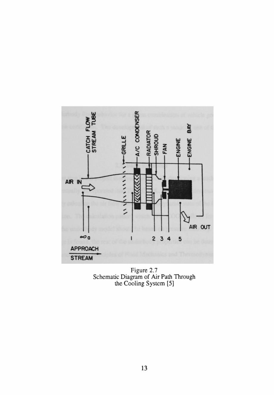
The numerical stations in Equation 2.2 can be located on Figure 2. 7 which is a depiction of
the air path for the Schuab and Charles study. The form of Equation 2.2 indicates that Kb
is proportional to the internal flow rate. Engine bay blockage is of interest because it is one
of the factors that determines fan efficiency. This study quantified Kb via tests in which
the fan was removed and air was drawn across the engine bay. These experiments
indicated that Kb had a constant mean value of 4.0 [5].
Schuab and Charles state that the value of Kb is dependent on the amount of
hardware in the flow path as well as on the separation between the engine front and the fan
exit. As the separation increased and the amount of hardware decreased, Kb generally fell.
12
~~ ""~ 0~ t~ .... ucn
AA IN¢
APPROACH
STREAM
~ ..J ..J ~ C)
l _, ,. ,. _, ,. ,.
~ z ~
~ a: CD
~9 u "" \&J ~0 z z ~
0 oa: ~
C!) C)
' ctX z z ct a: en ""'
AIR OUT
2 3 4 5
Figure 2.7 Schematic Diagram of Air Path Through
the Cooling System [5]
13
Their investigation also revealed that engine bay pressure levels tend to be positive. This
level increases with both radiator fan speed and freestream speed. Higher engine bay
pressures add significantly to the vehicle front end resistance [5].
This study and other similar research efforts have confirmed that the underbody
pressure and internal flow rate can definitely be influenced by parameters such as air dam
size, ground clearance, and engine bay flow resistance. While taking note of these effects,
however, the studies have not attempted to develop a physical model that could accurately
predict the underbody flow behavior for a given combination of vehicle geometry, external,
and internal flow conditions. The development of such a model is one of the main goals of
this project.
2.3 Basic Equations
The frrst step in the project involves theoretically developing a mathematical model
that can be eventually incorporated into TIU_COOL. This correlation can then be used to
more accurately calculate the air flow rate and thermodynamic state of the flow in the
underbody region. The calculation pattern which TIU_COOL follows for each component
indicates that the underbody model should be based on pressure recovery. Once the
pressure change is found, the rest of the underbody properties can be determined by
applying the fundamental principles of Fluid Mechanics and Thermodynamics [6]. The
first concept used is the Conservation of Mass Equation,
(pVA)e.rit = (pVA)u.ur· (2.3)
In Equation 2.3, the flow cross-sectional areas are assumed to have uniformity of
properties and a Steady State, Steady Flow (SSSF) incompressible process is assumed.
The second principle applied is the Force Momentum Equation,
14

The third principle applied is the Conservation of Energy Equation,
The fourth and final applied principle is the Entropy Production Equation,
The air is assumed to be an ideal gas with a constant specific heat with the Equations of
State as follows,
P = RpT,
(2.4)
(2.5)
(2.6)
(2.7)
(2.8)
(2.9)
The input parameters necessary to obtain a solution using the underbody correlation and the
equations listed above include inlet temperature and pressure, mass flow rate, and vehicle
speed.
2.4 Underbody Pressure Recovery Model
In developing the model for the underbody flow process, attention is focused on the
region depicted in Figure 2.8. The empirical underbody coefficients calculated from the
Taurus and F150 wind tunnel data were determined from the following relationship,
K =Po-~ u l.pVr2 .
2 0 (2.10)
15

Pr.exit
Pt,exit = Pr ,exit +~Plan
Figure 2.8 Generalized View of Engine and
Underbody Aow Region
16
The engine bay pressure change consisted of the momentum change across the region since
Kb was set to zero for all previous ITU_COOL calculations [2]. Therefore, these
relationships did not distinguish between the separate pressure loss effects of the engine
bay and underbody. A more detailed relationship can be obtained by considering the
pressure change from the fan exit to ambient conditions in terms of two pressure change
components as shown in Equations 2.11 and 2.12,
Pf,uil- Po= (Pt.m- ~) + (~- f»o), (2.11)
(2.12)
Equation 2.12 includes the assumption that the engine bay pressure loss is a function of the
radiator velocity while the underbody pressure loss is dependent on the freestream velocity.
Dividing Equation 2.12 by the freestream dynamic pressure yields the following
correlation,
p - P, ( )2 C = t.ail o = ~ K + K . p l ¥.2 v b u
2 p 0 0 (2.13)
Equation 2.13 is the equation of a line with slope Kb and intercept K" as shown in Figure
2.9. This correlation forms the basis for the numerical and experimental analysis which
will be detailed in the following chapters.
The accuracy of Equation 2.13 can be tested by plotting the underbody pressure
coefficient values against the square of the radiator to freestream velocity ratio values.
These quantities are obtained by running TIU_COOL with the Taurus and F150 wind
tunnel data to determine the grille and underbody pressure recovery results. The results of
this process are discussed in Chapter 3 of this report
17

Figure 2.9 Graphical Depiction of Underbody
Correlation
18

CHAPTER3
NUMERICAL ANALYSIS OF FORD TAURUS
AND F150WINDTUNNELDATA
This chapter provides a summary of the numerical and graphical analysis perfonned
on experimental wind tunnel data for two full-size Ford vehicles. The two vehicles
involved in these studies are a 1986 Taurus Sedan with a 3.0 L engine and an F150 pickup
truck.
3.1 Analysis Procedure
Each collection of vehicle data consists of experimental wind tunnel data gathered at
the Lockheed facility in Georgia The collection also includes ft.les which list the vehicle's
basic operating parameters and the geometry of the engine, fan, condenser, and radiator.
This data is then used as input in running the computer program TTU _COOL so
that the grille and underbody pressure recovery results can be calculated. The grille and
underbody data files generated by TTU_COOL are the source of the graphically analyzed
data. The primary goal of the Lockheed Wind Tunnel studies was to acquire flow rate and
pressure measurements for the flow of air through the grille, radiator, condenser, engine
bay, and underbody of the vehicle. This experimental data was then used to evaluate the
accuracy of 1TU_COOL's numerical predictions.
The graphical analysis of these data sets consists of plotting the underbody pressure
coefficient. CP, against the square of the ratio of radiator velocity to vehicle velocity for
each wind tunnel run. This analysis is intended to test the validity of the underbody
correlation presented in Equation 2.13. Therefore, the slopes of these figures represent Kb
and their intercepts indicate K". It should be noted that the value of CP given by
19

TfU_COOL and used in the plots represents the negative of the underbody pressure
coefficient as given by Equation 2.13.
After all of the individual plots are generated. plots are next made of the data runs
combined into groups corresponding to various configurations of air dams, spoilers, and
bumper openings. The aim of generating these grouped figures is to see if separating the
runs according to geometrical configurations would better collapse the plotted data towards
a curve fit line for that data set. In addition, it is hoped that these groupings will reveal
trends in the values of Kb and Ku for certain configurations.
3.2 Taurus
The first set of vehicle data examined is the Taurus collection. This data set
consists of experimental wind tunnel files and a vehicle data file named, LSWT[88-
288]W.DAT and VEH_90.CAR, respectively. As previously mentioned, CP versus
radiator velocity ratio squared plots were generated for each experimental run. Figure 3.1
is an example of a typical plot for the Taurus.
One characteristic which consistently appears on all of these figures is that the slope
of the least squares curve fit line for the given data is positive. This outcome is contrary to
the anticipated result that the curve fit would produce a negative slope. A negative slope
would correspond to the expected trend that as the vehicle speed increases or the radiator
velocity decreases. the underbody pressure would decrease.
Hand calculations performed using data from runs 100, 101, and 103 and the
Taurus vehicle file confirm that the values of Ku produced by Tru_COOL are correct in
both magnitude and sign. This contradiction between the expected and actual slope results
can be linked to two possible explanations. Either there is some sort of physical
phenomena present in the test data which can not be explained at present or there is some
erroneous experimental data
20

Cp 1r-----------------------------------------~
•
• 0.2~---------------------------------------------~
0~-----L------~-----L------~-----L------~----~
0 0.01 0.02 0.03 0.04 0.05 (Vr I Vcar)"2
Figure 3.1 Typical Taurus Plot of Underbody Pressure
Coefficient Versus Radiator Velocity Ratio Squared
21
0.06 0.07

A plot which combines all of the data points from runs 88 through 288 was the next
figure produced (Figure 3.2). Not surprisingly, the line curve fit to this collection
illustrates that the combined data is widely spread. This result demonstrates that although
there may be some erroneous data present, a further examination of the runs divided into
configuration groupings is warranted.
The first grouping consists of separating the runs according to whether the
openings are combined, runs 160 through 256, or isolated, runs 88 through 154 (Figures
3.3 and 3.4). A comparison of these two figures shows that the combinations data
collapses in agreement with the curve fit much better than did the data shown on Figure
3.2. However, an inspection of the isolated openings plot reveals no significant
improvement in terms of the degree of data spread in comparison to Figure 3.2. The
isolated case has greater underbody losses than those associated with the combinations
data. In addition, the isolated case has greater engine bay losses than those involved with
the combinations case.
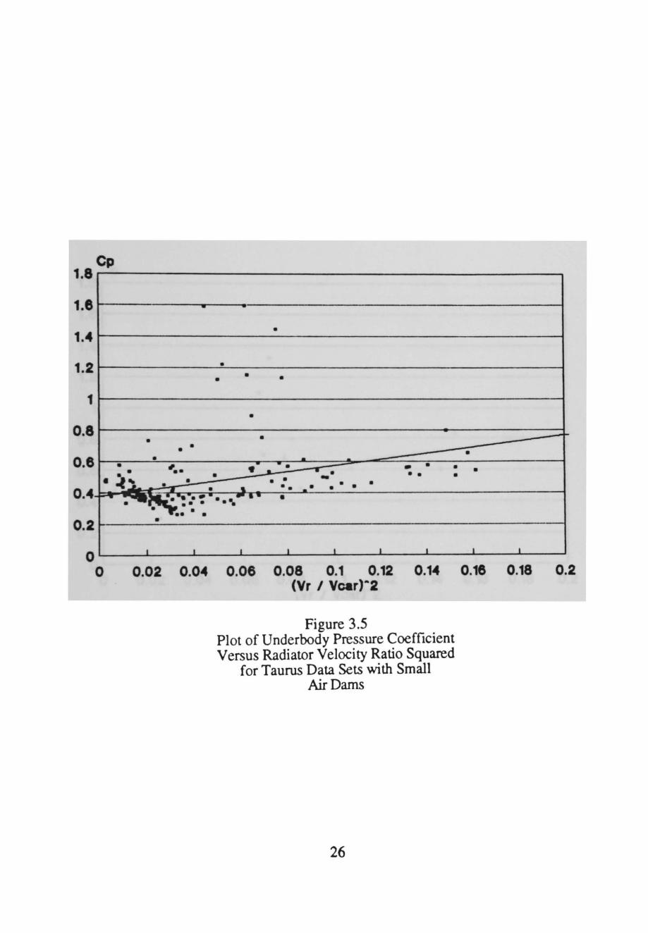
The second grouping divides the data into two groups according to whether a small
air dam, runs 88 through 256, or a large air dam, runs 258 through 288, was used in the
configuration (Figures 3.5 and 3.6). Both of these plots collapse the data to the curve fit
better than Figure 3.2, but not as well as the combinations of openings plot discussed
previously.
These same two groupings were further analyzed by evaluating the data and finding
the slope common to both while retaining the intercepts of each group (Figure 3.7). The
purpose of this calculation is to demonstrate that while both the large and small air dam
groups manifest similar trends in terms of slope, they differ from each other by an intercept
shift. The results show that the common slope for these groupings is 1.96 and that the
small and large dam cases have intercepts of0.377 and 0.437, respectively. Therefore, the
conclusion can be drawn that larger air dams produce lower underbody pressure levels.
22

Cp 1.8
1.8
1.4
1.2
1
0.8
0.8 • . . ' 8j.f4 0.4
0.2
0 0
~
•
• •
' •
-
• • • •
•
• • • • ~ ... •• • • .
~ .. .,. • ..... --... -.--• • • • • •• •
I
0.05
• •
•
•
• • ----. - • • • • - • • • • • • • • •• -· • • •
_l I
0.1 0.18 .___ __________ ...:...::(Vr I Vcar)"2
Figure 3.2 Plot of Underbody Pressure Coefficient Versus Radiator Velocity Ratio Squared
for all Taurus Data Sets Combined
23
-•
•
0.2

Cp 1.8
1.8
1.4
1.2
1
0.8
0.8
0.4
0.2
0
-• • • • •• •
~-- .. _.- ..... , .. ·~~·· • • •• •
I I I
-• --. • • • • • • • • • • -· • •
I I I I I _l
0 0.02 0.04 0.08 0.08 0.1 0.12 0.14 0.18 0.18 0.2 (Vr I Vcar)•2
Figure 3.3 Plot of Underbody Pressure Coefficient Versus Radiator Velocity Ratio Squared
for Taurus Data Sets with Combined Openings
24

1.8rCP __________________________________________ ~
1.8.---------~--------------------------------~
• 1.4r-----------------------------------------------~
0.8~------------------~~------------------------~
0.8~~~~--~~--~--------~--------------------~
• • • 0.2~----~·----------------------------------------~
o~------------~--~~--~------------~----~--~
0 0.02 0.04 0.08 0.08 0.1 0.12 0.14 0.18 0.18 0.2 (Vr I Vcar)•2
Figure 3.4 Plot of Underbody Pressure Coefficient Versus Radiator Velocity Ratio Squared
for Taurus Data Sets with Isolated Openings
25
Cp 1.8
1.8
1.4
1.2
1
0.8
0.8 •
0.4 _ _...
0.2
0
• • • • • .,,
• • •
•
I
-•
• • • •
•
• • •
-'·· .- --. • • • • • 'll •• ..... --... -.. • • • • •
•• • •
I I I
--• - - • • • • • • • • • - • • -· • •
I I I I I
0 0.02 0.04 0.08 0.08 0.1 0.12 0.14 0.16 0.18 0.2 (Vr I Vcar) .. 2
Figure 3.5 Plot of Underbody Pressure Coefficient Versus Radiator Velocity Ratio Squared
for Taurus Data Sets with Small Air Dams
26

Cp 1.8
1.8
1.4
1.2
1
0.8
0.8
0.4
0.2
0
: I"""
• • ~~
. .... •• • • •
I I
•
•
• --• • •
• • •
I I I I I 1 j
0 0.02 0.04 0.06 0.08 0.1 0.12 0.14 0.16 0.18 0.2 (Vr I Vcar)·2
Figure 3.6 Plot of Underbody Pressure Coefficient Versus Radiator Velocity Ratio Squared
for Taurus Data Sets with Large Air Dams
27

Cp 1.8
1.8
1.4
1.2
•
1
0.8
0.8
0.4
0.2
.±·.~ ~ -- .--:
0
+ •
• • + •
• • • • + • I
~.n .... _ -. .. • • ~ ~
• • • • • ·~:·.- ........ -If= •••• •
I I 1
•
•
+ .... + + •
• • - • • • • • • + - • • • • • . • • • •
I I I I I I
0 0.02 0.04 0.06 0.08 0.1 0.12 0.14 0.16 0.18 0.2 (Vr I Vcar)'"'2
• Small air dam + Large air dam
Figure 3.7 Common Slope Plot of Underbody Pressure
Coefficient Versus Radiator Velocity Ratio Squared for Taurus Data Sets
with Small and Large Air Dams
28

These results also indicate that the engine bay losses remain fairly constant between
dam sizes. The underbody pressure losses, however, increase for the larger dam sizes.
3.3 Fl50
The second set of vehicle data examined is the F150 collection. This set of data
consists of experimental wind tunnel data files and a vehicle data file named, PN96[ 109-
402] .D AT and F 150.CAR, respectively. In contrast to the Taurus data, all of the
individual plots for the F150 have the negative slopes which were expected as discussed
previously. Figure 3.8 is a typical plot of CP versus radiator velocity ratio squared for the
F150. Once again the generation of a plot for all the runs combined depicts a great deal of
data spread which indicates the need to divide the runs into separate groupings for further
analysis (Figure 3.9).
The frrst grouping examines configurations involving large, runs 264 and 269, and
small, runs 249 and 254, bumper mounted spoilers (Figures 3.10 and 3.11). An
examination of these figures reveals no real improvement in the degree of data spread in
comparison to Figure 3.9. However, the large spoiler results clearly depict lower
underbody pressures than those recorded using a small spoiler.
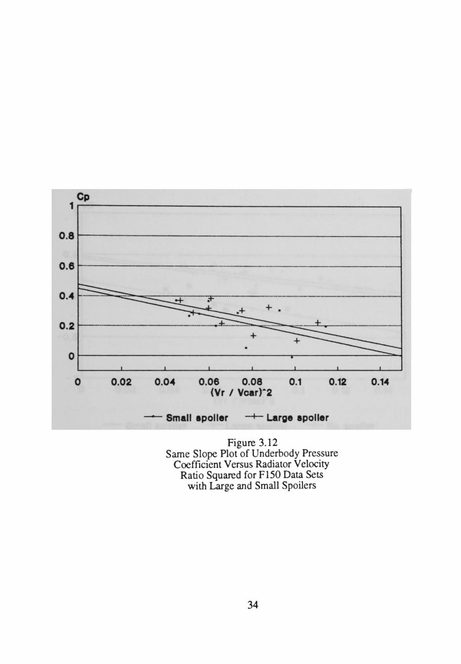
A plot was next made which combined the small and large spoiler data giving both
groups the same slope, -2.93, but different intercepts, 0.442 and 0.482, respectively
(Figure 3.12). In terms of collapsing the data, this figure is not as informative as was the
same slope plot generated for the Taurus small and large air dam cases. However, when
the spoiler groups were plotted along with similar configurations without a spoiler the shift
in the data caused by its presence can be clearly seen (Figure 3.13). An examination of this
figure illustrates the fact that the absence of a spoiler produces higher underbody pressures
than those configurations which include one.
29

Cp 1r---------------------------------------------~
0 0.02 0.04 0.08 0.08 0.1 (Vr I Vcar)'"'2
Figure 3.8 Typical Plot of Underbody Pressure
Coefficient Versus Radiator Velocity Ratio Squared for
the F150
30
0.12 0.14

Cp 1
o.e •
• • •• • • • ---· . --- .... ·" ......... ;;; . . - • . . . , . . . , "'·
• •
,. ••• ·-•••• • . -..; ~ • • • ••
• .. - •
• •• • • • • •• • .. . . ' • • ... ,. .. • • • • •• • • • .~· - • • 0 • • • . -. -
I• .~ -- • -· -o.e
-1 0
•
I
0.02
• ~ • -• •• • • •• • • • • • • • • • • • • • • • Ita. •
1 I I I
0.04 0.08 0.08 0.1 (Vr I Vcar)""2
Figure 3.9 Plot of Underbody Pressure Coefficient Versus Radiator Velocity Ratio Squared
for all Fl50 Data Sets Combined
31
• I •
•
1
0.12
•
• • -
I
0.14

Cp 1
0.5 ...._
0
-0.5
-1 0
I
0.02
• • - • • • --• • • •
I I 1 I
0.04 0.08 0.08 0.1 (Vr I Year )•2
Figure 3.10 Plot of Underbody Pressure Coefficient Versus Radiator Velocity Ratio Squared
for F150 Data Sets with Large Spoilers
32
-
_l_ I
0.12 0.14

Cp 1
o.e ~
0
-o.e
-1 0
--
I
0.02
• • • • •
• -- • •
I I I I
0.04 0.08 0.08 0.1 (Vr I Year )•2
Figure 3.11 Plot of Underbody Pressure Coefficient Versus Radiator Velocity Ratio Squared
for F150 Data Sets with Small Spoilers
33
I I
0.12 0.14
0 0.02 0.06 0.08 0.1 0.12 (Vr I Vcar) .. 2
- Small apoller -+- Large apoller
Figure 3.12 Same Slope Plot of Underbody Pressure
Coefficient Versus Radiator Velocity Ratio Squared for F150 Data Sets
with Large and Small Spoilers
34
0.14

Cp 1r-----------------------------------------------
0 + ·•
+ •
• -0.5~--------------------------------------------~
-1~----~----~------~----~----~----~------~~
0 0.02 0.04 0.08 0.08 0.1 0.12 0.14 (Vr I Vcar) .. 2
- Small apoller -+- Large apoller _._ No apoller
Figure 3.13 Plot of Underbody Pressure Coefficient Versus Radiator Velocity Ratio Squared
for F150 Data Sets with Large, Small, and No Spoilers
35
These two groupings do indicate that the large spoiler has a greater underbody loss
than that associated with the small one. The engine bay pressure losses are of
approximately the same magnitude for both cases.
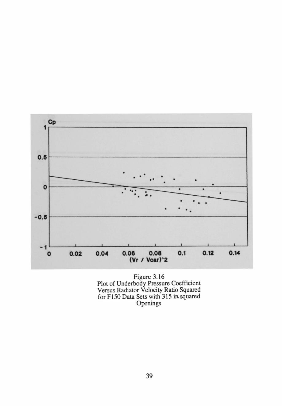
Another grouping that was analyzed consisted of dividing the runs according to the
areas of the above bumper and bumper openings. The area groups used were 105, 210,
315, 420, and 525 in. squared for either the two openings combined or for an opening
alone (Figures 3.14, 3.15, 3.16, 3.17, and 3.18). Only the 525 in. squared configuration
depicted on Figure 3.18 shows a marked improvement in collapsing the data close to the
curve fit line.
One interesting trend can be spotted by comparing the 210, 315, and 420 in.
squared plots (Figures 3.15, 3.16, and 3.17). As the opening size increases, the CP value
decreases and consequently the underbody pressure increases. This trend indicates that
both the engine bay and underbody losses decrease as opening sizes are reduced.
The fmal set of data examined compared a small air dam, run 284, with a large air
dam, run 179 (Figure 3.19). An examination of this plot reveals the same trend that was
found when the Taurus data was compared on the basis of dam size. The large dam again
produces lower underbody pressures than does the small one. In addition, the large dam
produces greater underbody losses than does the small one. The engine bay losses,
however, are of the same magnitude for both cases. The values of Kb and K" are larger
for the Fl50 dam cases than for the similar arrangements on the Taurus.
The overall cp intercept difference between the two dam sizes, however, is
apparently greater for the F150 than it was for the Taurus. This result occurs in spite of the
fact that the heights of the small and large air dams used on both vehicles were the same.
36

0.5
0
-0.5
-1 0
. • •
• • • • • . . .. • ' ••• • •• • • • • • • .- • • • -
• •
•
I
0.02
• • • •
• • • • •
•
1 I I 1
0.04 o.oe o.oa 0.1 (Vr I Vcar)•2
Figure 3.14 Plot of Underbody Pressure Coefficient Versus Radiator Velocity Ratio Squared for F150 Data Sets with 105 in. squared
Openings
37
I I
0.12 0.14

Cp 1
0.5
-0
-0.5
-1 0
-
I
0.02
• • •
• • .
•
l
0.04
• • • • •
• • • • • - • • ---.. - -• • •
• • •
• • •
I I l _l
0.06 0.08 0.1 0.12 (Vr I Vcar) .. 2
Figure 3.15 Plot of Underbody Pressure Coefficient Versus Radiator Velocity Ratio Squared for Fl50 Data Sets with 210 in squared
Openings
38
- -
I
0.14
Cp 1
0.5
-0
-0.5
-1 0
I
0.02
• • • • • •• • • • • •• • •
• • • -. • • • •
• • • •
I I l I
0.04 0.08 0.08 0.1 (Vr I Vcar)•2
Figure 3.16 Plot of Underbody Pressure Coefficient Versus Radiator Velocity Ratio Squared for F150 Data Sets with 315 in squared
Openings
39
• •
•
• -
I I
0.12 0.14

Cp 1
o.e
0
-o.e
-1 0
I l
0.02 0.04
• • •
• • •
•
l I I
0.08 0.08 0.1 (Vr I Vcar)•2
~--------------------~~
Figure 3.17 Plot of Underbody Pressure Coefficient Versus Radiator Velocity Ratio Squared for F150 Data Sets with 420 in squared
Openings
40
•
•
l l
0.12 0.14

-1~----~----~----~----~~----~----~-----L~
0 0.02 0.04 0.08 0.08 0.1 (Vr I Vcar)•2
Figure 3.18 Plot of Underbody Pressure Coefficient Versus Radiator Velocity Ratio Squared for Fl50 Data Sets with 525 in squared
Openings
41
0.12 0.14

Cp 1
0.5 ~
0
-0.5
-1 0
I
0.02
• • ..L. +.
~ + +
I I l I l
0.04 0.08 0.08 0.1 0.12 (Vr I Vcar)•2
--- email dam -4- large dam
Figure 3.19 Plot of Underbody Pressure Coefficient Versus Radiator Velocity Ratio Squared
for F150 Data Sets with Small and Large Air Dams
42
•
I
0.14

3.4 Summary
The analysis results discussed above show that the wind tunnel data for both the
Taurus and F150 can be successfully correlated according to various geometrical
configurations. An examination of plots of CP versus radiator velocity ratio squared for
each vehicle demonstrated that the underbody correlation presented in Equation 2.13 is
valid. This validity was demonstrated by the nature of the trends in Kb and K" found for
different dam sizes, frontal opening areas, and spoiler sizes. For example, the small and
large spoiler results for the F150 indicated that K" grew as the spoiler size increased.
However, the engine bay resistance was relatively unaffected by this change. Both of these
trends conform to the expected flow behavior in the engine bay and underbody of a vehicle.
Therefore, the material presented in this chapter proves that the underbody correlation is an
appropriate basis upon which to conduct further experimental analysis and study.
43

CHAPTER4
EXPERIMENTAL APPARATUS AND TEST PROCEDURE
This section provides a description of the wind tunnel test facility utilized for this
project. In addition, the features of the experimental model and its associated
instrumentation are discussed. Finally, the calibration and test procedures are explored in
depth on a step-by-step basis.
4.1 Wind Tunnel Test Facility
The experimental tests for this study were performed in the Eiffel type wind tunnel,
as depicted in Figure 4.1, at the Texas Tech Mechanical Engineering Laboratory. This
forced draft tunnel has an open throat configuration and is capable of producing flow rates
of up to 65,000 cfm. For this series of experimental tests, the model was placed at the
tunnel's exit nozzle where the maximum velocity obtainable is approximately 78 ftls. The
exit velocity is adjustable via movable damper vanes on the inlet to the wind tunnel blower.
A 4 ft. wide by 8 ft. long plywood platform was placed at the 3 ft. high by 4 ft.
wide nozzle exit to support the model in an open test section. Previous studies on this
configuration have shown that the vertical and lateral flow velocities are fairly uniform
across the test section [7]. In addition, the tunnel turbulence levels were found to be
relatively low.
Therefore, the tunnel velocities involved in the experimental runs were essentially
constant along both the vertical and horizontal axes of the model. This fact indicates that
the static pressure gradient along the axis of the tunnel is negligible which was one of the
advantages of utilizing an open test section [7].
The value of the tunnel blockage ratio for this experiment was calculated to be
0.065. This ratio is smaller than the blockage that would have been encountered with the
44

Diffuser \ ,/ ;..-Settling Chamber J Nozzle
-· ~--~ /
../y K ........ t--~ ·
......=-... 1 C I
17' ~ I [I i1l t- v 1-
\ \.\. 7; r..... t"- v ....... ~ v f': ~P" ~
~ v I t-- .._It ~ I
38'
flow 01rect1on
Figure 4.1 Schematic of Texas Tech Wind Tunnel [7]
45

same model in a closed parallel test section. The smaller blockage value is another of the
advantages of using an open test configuration.
4.2 Experimental Model
The model used for this project was a modification of an existing apparatus that was
constructed and tested by C.M. Roseberry to investigate ram recovery coefficient
correlations. This model was built to provide a 0.2-scale representation of a generically
shaped automotive front end with alterable front and bottom openings and an adjustable air
dam. Two interchangeable bluff and streamlined front ends were also fabricated so that the
effects of those variables could be evaluated. The remainder of the model consisted of an
elongated 0.25 in. thick plywood duct connected to an adjustable 0. 75 in. thick plywood
ground plane.
The duct was included to simulate the engine compartment and to provide a means
of connecting the model to a centrifugal blower. This blower was used to reproduce the
combined effects of the radiator fan and ram air in inducing flow through the engine bay to
the underbody. A rectangular to round transition was used to connect the blower to the
duct via flexible plastic tubing. Three manifolded pressure taps were placed in the engine
bay to record the pressure levels. The duct length was such that the effects of any upstream
blower disturbances upon the internal flow were negated.
The purpose of supporting the model on a ground plane was to reduce the boundary
layer thickness that would have been encountered had the model been attached directly to
the test platform [8]. For this series of tests the groundplane was modified by placing rigid
steel legs at the comers with a movable rocker installed at the center of each side. This
configuration provided for more convenient levelling of the ground plane. The height of the
rockers was set ftrst and then the clamped rigid legs were adjusted until a level position was
achieved.
46

Figure 4.2 is a diagram of the apparatus after the various modifications for this
project were completed. Two variations of a streamlined nose were built since the bluff
nose was not used for these tests. Roseberry found that the bluff front end tended to
develop a large separation bubble which completely covered the bottom opening [8]. This
behavior renders any data gathered for an isolated bottom opening invalid.
One of the primary alterations consisted of drilling 51 holes centered along the
groundplane beginning from 9.5 in. in front of the model to 32.5 in. behind it Brass
tubing of 0.03125 in. in diameter was inserted into these holes to provide taps so that the
underbody pressure distribution could be recorded along the centerline of the model.
A second modification involved placing a vane anemometer at the rear of the model
to provide a means of measuring the underbody flow rate. Clear plastic panels were
attached along the length of both sides of the model to prevent the underbody flow from
exiting via that route. The legs supporting the model were sealed at the groundplane slots
with rubber gaskets to prevent any leakage. A slotted block with a spring loaded flap was
installed at the rear of the model to route the underbody flow into the anemometer inlet
This arrangement provided only two avenues of escape for the underbody flow. The flow
had to leave through either the anemometer or out the front of the model beneath its nose.
A section of cardboard honeycomb (0.25 in. wide cells, 2 in. long) and fme metal
screen (36 mesh, 59% open area) was placed in the duct upstream of the engine bay taps.
The reason for this arrangement was to dampen any turbulent flow disturbances in the duct
originating from the blower. This dampening was necessary so that steady engine bay
pressure measurements could be taken.
The final change undertaken was to reverse the direction of the blower output so
that it produced flow into the duct. This alteration was required in order to reproduce the
flow through the engine bay to the underbody. This change was necessitated because the
47

WIND TUNNIL IXIT NOZZLI
INGINI IM PR188URI TAN PITOT-auriC PROlE
DIRECTION ltOTTOM OftENING
HONI!~OMI I 8CREEN
QROUNDPLANE AIR DAM
OPIN TilT PLATFORM
ROCKER
Figure 4.2 Experimental Model
48
I LOWER OONNI!OTION
ANIMOMET!R

model frontal openings were excluded for this experiment in order to focus attention on
flow behavior through the underbody opening.
An aluminum air dam was constructed with dimensions of 0.625 in. in height and
13.5 in. in width. The air dam was affixed to the underbody opening's front edge and it
extended completely across the model's underside. A fmely meshed screen (36 mesh, 59o/o
open area) was used to cover this opening. This screen was installed to reproduce the
pressure drop associated with the engine bay loss coefficient, Kb. The size of the bottom
opening in terms of both length, 0.64 in., and width, 11.5 in., was kept constant for all
tests. The opening was located 4.5 in. behind the nose of the model.
The model components that could be altered included: frontal nose shape, air dam
height, ground clearance, and bottom screen density. Once the combination of parameters
was set, the tests were conducted by operating the tunnel at 6 nominal speeds: 0, 15, 25,
40, 50, and 60 ft/s. For each of these speeds, the blower setting was varied through 10
nominal flow rates: 0, 20, 40, 60, 80, 100, 120, 140, 160, and 180 scfm. Thus a single
test run, as recorded by the data acquisition program, consisted of a particular combination
of model component variations, a fixed wind tunnel speed, and a blower flow rate setting.
4.3 Instrumentation
The underbody and engine bay pressure taps were connected via 0.0625 in. inner
diameter plastic tubing to a Scanivalve Model J scanning valve with a solenoid drive. This
instrument was controlled by commands issued from a Scanivalve ITF-488 interface
controller and a Scanivalve CTLR 10P/S2-S6 solenoid controller. These units in turn
received digital commands from a Metrabyte DASH-16 Analog to Digital (NO) converter
board installed in a Zenith ffiM-compatible personal computer.
The common pressure port of the scanning valve was connected to a V ali dyne
Model DP-45 differential pressure transducer. A second identical transducer was used to
49

record the differential pressure across the blower laminar flow element (Meriam Model
50MC-2-4) so that the flow rate entering the model could be calculated.
A Validyne Model MC1-10 carrier module with Validyne Model CD-18 signal
demodulators installed provided the source excitation for the transducers. This unit also
delivered a linearized output voltage corresponding to the pressure reading to the ND
board. Finally, the vane anemometer was connected to the computer through the counter
input terminals on the AID board.
Figure 4.3 is a schematic of the connections between the instrumentation and the
model pressure measurement ports. The scanning valve common port was connected to the
high side of the first transducer while the low side was linked to the static pressure port on
the wind tunnel pi tot-static probe. Port number 0 was used to keep track of the span
measurement ( P10taJ - ~tat) from the tunnel probe. Port number 1 was connected to the
manifolded engine bay pressure taps while ports 2 through 36 were linked to the various
groundplane underbody taps.
The high and low sides on the second transducer were connected to the high and
low pressure ports on the blower laminar flow element. In terms of the AID connections,
channel! was used for the scanning valve readings while channel2 was reserved for the
laminar flow element data.
The anemometer was connected to the ND counter 0 input terminal via a square
wave generator box. This box was powered by a standard 9 volt battery and produced a
square wave signal which corresponded to the anemometer reading. This signal was sent
to the AID board which interpreted it in terms of a pulse count.
The anemometer calibration procedure utilized the blower as a flow source for the
instrument via a connection with flexible plastic tubing. The blower was run at a known
flow rate while the computer recorded the corresponding total pulse count in one second.
50

SQUARE WltiE
GENERATOR
TO ANEMOMETER
COMPUT!R
DASH-18 A/D
BOARD
SIGNAL CONDITIONE
CH J CH 1
ItT J ItT 1
SCANNING CONTROLLER
UNIT
&CANNING "'LYE
TO LAMINAR FLOW ELEMENT TO ltiTOT-I'IATIC ltROII
Figure 4.3 Instrumentation Schematic
51
TO MOHL ltRE88URE
TAitl

This pulse reading could then be used as a basis for calculating the flow rate corresponding
to any pulse count recorded in the same time period.
The blower apparatus consisted of an impeller that was belt driven by a Baldor 1.0
Hp DC motor with a U.S. Controls speed controller. The blower speed was set manually
using the non-dimensional dial on the controller unit along with an oil-filled manometer.
Finally. the wind tunnel speed was manually set by adjusting the damper vanes at the
tunnel impeller intake.
4.4 Experimental Procedure
The experimental procedure was divided into two separate operations. The frrst one
involved calibrating the two pressure transducers by establishing their respective zero and
span settings via the controls on the V ali dyne demodulator units. In addition, the
anemometer was calibrated via the procedure described previously.
The second operation consisted of actually running the test and gathering data from
the various pressure ports and the anemometer. A C language computer program was
written to perform these tasks interactively with the user by following the steps listed
below.
1. The model and groundplane were secured and levelled into the position desired.
2. The tunnel and blower were activated and their speeds were manually set and adjusted
by using oil-filled manometers
3. The computer program, named STDYTEST.C, was activated to begin the calibration
procedure.
4. With the high and low sides of both transducers left open to atmospheric pressure, the
Validyne output was set to zero using the zero potentiometer on each channel.
52

5. The high and low sides of the Scanivalve transducer were linked to the common port
and the static pressure port of the pitot-static probe, respectively. The high and low
sides of the blower transducer were connected to the corresponding ports on the
laminar flow element
6. The output from each transducer was adjusted via the span potentiometer on the
V ali dyne to approximately + 4.5 volts within +1- 0.003 volts. The program then
recorded the span reading for each transducer.
7. The magnitude of the span readings in in. H20 were next entered by using the readings
from the corresponding manometers.
8. The procedure described in step 4 was repeated and the program read in the
corresponding zero readings (0.000 volts +1- 0.003 volts).
9. To begin the testing phase, the program required the user to enter the name of the
output fue, the tunnel temperature, tunnel pressure, run number, and any comments
regarding the test run. Knowing the tunnel dynamic pressure in in. H20, the tunnel
speed was next calculated.
10. The program next read in the pressure differential from the blower and calculated the
corresponding flow rate in scfm using the temperature and pressure corrected
calibration curve provided in the Meriam manual.
11. The program then read in the anemometer reading in tenns of a pulse count and
calculated the corresponding underbody velocity.
12. The scanivalve was then issued a 'Home' command to begin the pressure
measurements at port 0.
13. The program then read in the pressure differential (Ppon- ~~ar> for each port at a
frequency of 40 Hz for a total of 5 seconds.
14. Next, the scanivalve was issued a 'Step' command to advance the valve to the next
port.
53

15. Steps 13 and 14 were then repeated until all ports had been stepped through. At this
point, the data gathering process was completed.
16. The last step in the program calculated the pressure coefficient values, using the
relationship
C = (Pporr- zero) P (span- zero)· (4.1)
17. The user was fmally given the option of either running another test starting with step
10 or terminating the test program.
The procedure described in step 6 had to be modified for the lower tunnel speeds.
At lower speeds, the span setting had to be reduced below 4.5 volts in order to keep the
engine bay pressure readings within the 5.0 volt range of the AID board. This modification
explains why the engine bay CP values discussed in Chapter 5 for the lower tunnel speeds
were so large.
Throughout the running of the program, the relevant experimental parameters and
results were written to the screen and to file storage for later reference. The purpose of this
procedure was to facilitate the management of the test. In addition to the primary data, such
as pressure coefficients, intermediary quantities such as density were also recorded so that
the user could track down any calculation discrepancies.
The accuracy of the experimental system, in terms of pressure and anemometer
readings, was checked at regular intervals between test runs to insure the validity of the
results. This process consisted of comparing the predictions of the computer
measurements with the actual readings obtained by using manometers for the pressure
readings and a frequency counter for the anemometer.
54

CHAPTERS
DISCUSSION OF EXPERIMENTAL RESULTS
5.1 Introduction
The experimental data reduction and graphical analysis for this project has two
objectives. One aspect of interest is to determine the validity of the engine bay and
underbody pressure drop correlations presented in Chapter 2. Another objective of the
analysis is to gain a better understanding of the nature of underbody flow behavior. The
analysis is executed in a manner such that the interaction effects of the internal and external
flows in the underbody region are revealed. Sections 5.2 to 5.4 describe the graphical and
numerical analysis results for the experimental wind tunnel data.
5.2 Anemometer Results
Figure 5.1 is an illustration of the average underbody velocity, ~'measured by the
anemometer versus the average internal or radiator velocity, V,., measured via the laminar
flow element. Each set of symbols corresponds to a line of constant freestream velocity
ranging from 15.48 ft/s to 59.86 ft/s. The relationships used to calculate ~ and V,. are
given by Equations 5.1 and 5.2,
v =~ " A., '
V =~ r •
~nt
Parameters ~ and {1 represent the underbody and internal volumetric flow rates,
respectively. The quantities A., and ~nt are the cross-sectional underbody and interior
areas of the model, respectively.
55
(5.1)
(5.2)

18
14
12
10
8
e 4
2
0
Vub (ft/a)
. ~ tl
~
0
ll ll
* * l
"'"
y 0
D D
+ 41.71 ft/a
o 14.14 ft/a
I
2
ll ll ll A Q
ll
* • * • * • "T + + + + +
0 0 0 0 0 0 0
0 D D -u
0
I I
4 8 Vr (ft/a)
* 11.71 ft/a
ll 18.84 ft/a
o 11.10 ft/a
Figure 5.1 Average Underbody Velocity Versus
Average Internal Velocity
56
A
• +
1:f 0
8
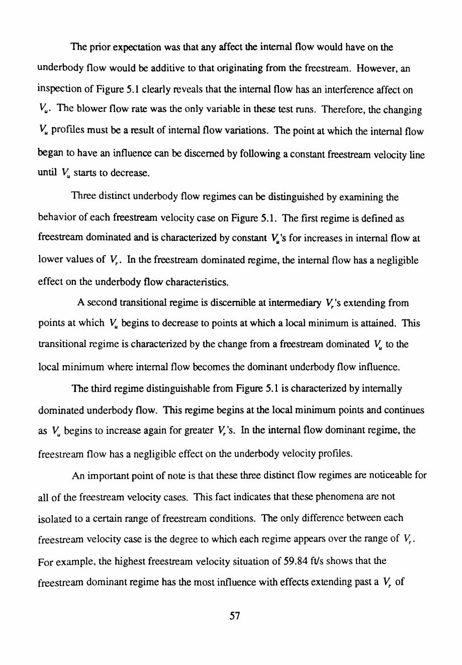
The prior expectation was that any affect the internal flow would have on the
underbody flow would be additive to that originating from the freestream. However, an
inspection of Figure 5.1 clearly reveals that the internal flow has an interference affect on
V:. The blower flow rate was the only variable in these test runs. Therefore, the changing
V: proftles must be a result of internal flow variations. The point at which the internal flow
began to have an influence can be discerned by following a constant freestream velocity line
until V: starts to decrease.
Three distinct underbody flow regimes can be distinguished by examining the
behavior of each freestream velocity case on Figure 5.1. The first regime is defined as
freestream dominated and is characterized by constant V., 's for increases in internal flow at
lower values of V,.. In the freestream dominated regime, the internal flow has a negligible
effect on the underbody flow characteristics.
A second transitional regime is discernible at intermediary V,. 's extending from
points at which V., begins to decrease to points at which a local minimum is attained. This
transitional regime is characterized by the change from a freestream dominated V., to the
local minimum where internal flow becomes the dominant underbody flow influence.
The third regime distinguishable from Figure 5.1 is characterized by internally
dominated underbody flow. This regime begins at the local minimum points and continues
as V: begins to increase again for greater V,. 's. In the internal flow dominant regime, the
freestream flow has a negligible effect on the underbody velocity proftles.
An important point of note is that these three distinct flow regimes are noticeable for
all of the freestream velocity cases. This fact indicates that these phenomena are not
isolated to a certain range of freestream conditions. The only difference between each
freestream velocity case is the degree to which each regime appears over the range of V,..
For example, the highest freestream velocity situation of 59.84 ft/s shows that the
freestream dominant regime has the most influence with effects extending past a V,. of
57

4 ft/s. In contrast, the lowest freestream velocity case of 15.84 ft/s illustrates that the
internal flow dominant regime exhibits the primary effects, noticeable even for small
increases in V . r
Figure 5.2 was generated in order to gain a better understanding of the nature of the
internal flow interference upon the underbody flow. This figure is a depiction of the ratio
of internal flow rate to underbody flow rate exiting the rear of the model versus V,.. The
points at which each freestream velocity case crosses the flow rate ratio of one line indicates
that the internal flow rate is exceeding the underbody flow rate exiting the rear of the
model. Since the only other avenue of escape is out the model front, those points
correspond to cases where a significant portion of the underbody flow is leaving via that
opentng.
The three regimes can be located on Figure 5.2 by the position of each freestream
velocity case relative to the flow rate ratio axis. Therefore, the freestream dominant points
are below the ratio of one line, the transitional regime is positioned just on the line, and the
internal flow dominant points are all located above the line.
Before concluding the discussion of Figure 5.2, two other points of significance
must be explored. First, an examination of the figure illustrates that the majority of the data
points are located in the freestream dominant and transitional regimes. The freestream
dominant regime is of primary interest in terms of aiding vehicle design since the
transitional and internal flow dominant cases are not desirable phenomena. That type of
flow reduces the cooling system efficiency by obstructing the cooling flow path underneath
and inside the vehicle. In addition, heated air would probably be recirculated into the
engine compartment further impairing the cooling process.
The second significant point is that for the lowest freestream velocities an
asymptotic limit is reached for the higher values of V,.. This phenomena indicates that for
58

VrAI/VubAub s
2.8
2
1.5
1
0.5
0 0
0
0 []
0 i •
+ 41.71 .. ,.
<> 14.14 ft/e
0 0 0
0 0
0 0
0
n b . T
0 + + •
0 + -...- &a
• 6
+ ,..• 6 .. i ~
I I I
2 4 8 Vr {ft/a)
• &1.78 .. ,.
A &1.84 ft/e
o 1&.&0 ft/a
Figure 5.2 Ratio of Internal Flow Rate to Underbody
Flow Rate Versus Average Internal Velocity
59
0
0
+
• A
8

certain conditions further increases in V,. lead to a constant percentage of the internal flow
exiting out beneath the model's nose.
Figure 5.3 is a non-dimensional plot of the data presented in Figure 5.2. On this
figure. the internal velocities are divided by the corresponding freestream velocities for each
case. The data does collapse along a single line indicating that this non-dimensionalization
was appropriate. The three regimes can again be located by the position of the data points
relative to the flow rate ratio axis as was described previously for Figure 5.2.
5.3 Engine Bay Pressure Measurements
Figure 5.4 is an illustration of the engine bay pressure measurements versus
radiator velocity ratio squared. This plot is the same as those generated for the F150 and
Taurus wind tunnel data discussed in Chapter 3. The purpose of producing this figure is to
see if the correlation derived and applied for the existing wind tunnel data is still accurate
and applicable for the data collected in this experiment.
An inspection of the data shown on Figure 5.4 illustrates the linear distribution of
the engine bay pressure points along a constant slope line. However, the three flow
regimes cannot be discriminated individually by their graphical differences. An
examination of Figures 5.2 and 5.3 demonstrates that the freestream dominant points are of
primary interest. Therefore, the presentation of data shown in Figure 5.4 can be narrowed
to a smaller range of radiator velocity ratio squared values without losing any information
of value.
Figure 5.5 is a plot of the same data presented in Figure 5.4 with the radiator
velocity ratio squared axis limited to 0.035. This ratio is determined by where the
preponderance of the freestream dominant data points are located on Figure 5.3. An
examination of this figure more clearly demonstrates the graphical differences between the
60

VrAr/VubAub a
2.&
2
1.&
1
o.e
0 0
0 l-
.A* __ ,.
I
0.1
+ 41.78 ft/a
o 14.84 ft/a
D D D
tJ 0
0
OD
no + T
*&*
I I I
0.2 0.3 0.4 Vr I Vo
• 11.78 ft/a
6 11.84 ft/a
D 11.10 ft/1
Figure 5.3 Ratio of Internal Flow Rate to Underbody
Flow Rate Versus Ratio of Average Internal Velocity to Freestream
Velocity
61
D
0.5
25 Cp(bay)
20
15
10
• • ~
xJ1. •
-~ I 0 0 o.oe
• 41.74 ft/a
o 11.81 ft/a
•
)(
~
•
I I
0.1 0.15 (Vr I Vo)•2
+ 11.71 ft/a
x 11.41 ft/a
Figure 5.4
)(
1
0.2
• 14.177 ft/a
Engine Bay Pressure Coefficient Versus Radiator Velocity Ratio Squared
62
....
0.25

3.5 Cp(bay)
• -t-o x.+n
3
2.5
2
1.5
1
0.5
0 0
;lc+c
I
0.005
• 41.74 ft/a
a 11.88 ft/a
• ,.. •
• ·+
X • +
• +n 0 •
0
I I I I I
0.01 0.015 0.02 0.025 0.03 (Vr I Vo)"'2
+ &1.78 ft/a
x 1&.48 ft/a
• 24.177 ft/a
Figure 5.5 Engine Bay Pressure Coefficient Versus
Limited Radiator Velocity Ratio Squared
63
•
0.035
three regimes in tenns of their differing slopes. The freestream dominant regime is
exhibited in the radiator velocity ratio squared range from 0.0 to 0.002. The transitional
regime is located between ratios of 0.002 to 0.015 while the internal flow dominant cases
are found from ratios of 0.015 to 0.035.
Recall that the slope of these data groupings represents Kb and the intercept
signifies Ku. An inspection of Figure 5.5 demonstrates that the freestream dominant case
has the highest Kb and an intennediate Ku. The transitional regime has the lowest value of
Kb and the highest value of Ku. Finally, the internal flow dominated portion has the
lowest Ku and an intermediary value of Kb.
5.4 Underbody Pressure Results
Figure 5.6 is a depiction of the underbody pressure distributions for a freestream
velocity of 41.76 ft/s. The symbols represent lines of constant radiator velocity ratio
squared. Comparisons can therefore be made with Figures 5.4 and 5.5. Recalling that the
three regimes were described in Figure 5.5 by ranges of radiator velocity ratio squared, the
regimes can also be identified on Figure 5.6 by those same values.
The reason that the underbody pressures are generally positive is due to the
considerable downstream blockage of the model. Most of the blockage can be attributed to
the presence of the plastic side panels and the anemometer duct. Vehicle underbody
pressures are normally below ambient levels along the length of the car. The model
pressure measurements are accurate in terms of their distribution patterns, but they are
shifted into the positive range by the blockage effects.
Each data point corresponds to the groundplane tap depicted on the model schematic
directly above the plot. The precise location of the 20 taps used is shown in terms of the
distance in inches from the first tap. There are three distribution regions in Figure 5.6 that
best illustrate the underbody pressure behavior of each flow regime. These regions consist
64

t I llllllll
Cp
1.4
1.2
1
0.8
0.8
0.4
0.2
'
0 0
.. - • lC. .... i a D •
• • • •
I I
2
• (Vr/Vo)•J•O.OSSO
a cvr/Vo)·a·o.oose
0 l'-Kl
• •
• • •
• • 8 D
+ ll - 0 "'
* • ~~~~~~~o~
• ••• tti • ~ ~ ~ • • 0 . A
• v v
• * • • tl • • • •
I I I I I I
e a 10 12 14 18 Tap poaltlon (lnchea)
• (Vr/Vo)•2•0.0202
+ (Vr/Vo)·a·0.0004
Figure 5.6
0 (Vr/Vo)•2•0.010S
x (Vr!Vo)·a·o.oooo
Underbody Pressure Coefficient Distribution for Freestream Velocity of 41.76 ftls
65
!
0
• •

of the taps directly beneath the air dam and bottom opening, the taps extending back from
the bottom opening, and the taps located in the area between the air dam front and the nose.
The internal flow dominant case exhibits a pressure peak in the opening region
caused by the impingement of the internal flow on the taps. This case shows a
considerable deviation from the freestream dominated regime for the taps located behind the
opening. This behavior indicates that the internally dominated cp distribution in this area
scales better with internal flow rate than it did with the freestream velocity. Finally, the
distribution in the nose region depicts low pressures consistent with higher velocities as the
underbody flow exits out the front of the model.
The transitional regime also has a pressure peak in the outlet region but it is much
diminished compared with that of the previous case. In addition, the peak is deflected back
along the taps due to the increased influence of the freestream velocity. The distribution
behind the opening exhibits scatter which indicates that the CP values still do not scale well
with freestream velocity. However, the data points collapse closer to the freestream
dominant cp 's than did those for the internally dominated case.
The nose measurements for the transitional situation indicate higher pressures
corresponding to a stagnation point This phenomena can be explained by recalling that for
the transitional case the freestream and internal flow effects are interacting in opposite
directions beneath the nose. These two opposing flows combine to create a high pressure
and low velocity region.
The freestream dominated regime does not demonstrate any noticeable peak in the
opening region. Instead, the distribution exhibits a decrease corresponding to an
acceleration of the flow as it passes around the edge of the air dam. The taps aft of the
opening region illustrate that the CP 'sin this region collapse to a single line that slowly
rises due to frictional effects. Therefore, the CP values in this case do scale well with the
freestream velocity as was expected.
66

Finally, the nose pressures are lower indicating that the velocities are higher in this
area than those associated with the transitional case. Recall that the flow direction for this
case is towards the rear of the model as opposed to the internally dominated case where the
flow heads towards the front.
The plots shown on Figures 5.7 and 5.8 depict the underbody pressure distribution
results for freestream velocities of 49.40 ft/s and 59.84 ftls, respectively. The validity of
the pressure distributions can be confrrmed by comparing results for equal values of
radiator velocity ratio squared. This agreement can be seen by comparing the pressure
distributions for ratio values of 0.0202 between Figures 5.6 and 5.7. This comparison
confirms the fact that the pressure distribution results are independent of wind tunnel
speed.
1be internally dominant regime continues to exhibit a pressure peak in the opening
region but the increased freestream velocities diminishes its magnitude. This case and the
transitional regime also continues to show scattered CP values in the region aft of the
opening corresponding to non-scaling with the freestream velocity. However, as the
freestream velocity increases these two cases show a greater degree of scaling than can be
found in Figure 5.6. Finally, the nose stagnation point associated with the transitional
regime is still apparent for both of the higher freestream speeds.
Figure 5.9 is a generalized illustration of the underbody pressure distribution
characteristics of the three flow regimes. An examination of this figure provides a clearer
view of the distributions associated with each regime independent of freestream speed.
5.5 Summary
This section detailed the numerical analysis of experimental wind tunnel data for the
model described in Chapter 4. One section of the analysis was devoted to testing the
validity of the underbody correlation given in Chapter 2. The plots of engine bay pressure
67
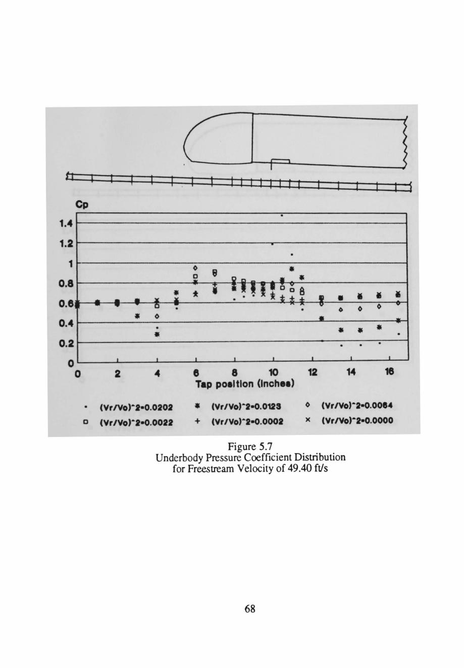
tJ
Cp
1.4
1.2
1
0.8
0.8
0.4
0.2
·~
0 0
•
I I I I t I l 1
•
. •
0 e • 2 0 • •
: t i i1l i: 0 0 8 • ... - • lC . . . t ~ ~ • • • - -.- .. 0 ~ " v 0 • • 0 0 • 0 • • • • • •
• • •
I I I I I I I I
2 4 e 8 10 12 14 18 Tap poll tlon (lnchea)
(Vr 1Vo)·a·0.0202 • (Vr/Vo)•t•0.012S
+ (Vr /Vo)·a-o.oooa
0 (Vr/Vo)·a-o.OOI4
x (VriVo)•t-o.oooo
Figure 5.7 Underbody Pressure Coefficient Distribution
for Freestream Velocity of 49.40 ftls
68
• v
--......-•

II 11111111 Cp
1.4
1.2
1
0.8
0.8
0.4
0.2
0 0
' 8 •
• • • • •
• • • •
2 8 8 10 12 18 Tap poaltlon (lnchea)
• (Vr/Vo)•2•0.01SI
a (Vr/Vo)•2•0.0017
• (Vr/Vo)•2•0.0018
+ (Vr /Vo)•J•O.OOOJ
<> (Vr/Vo) .. J-0.0048
x (VriVO) .. J•O.OOOO
Figure 5.8 Underbody Pressure Coefficient Distribution
for Freestream Velocity of 59.84 ft/s
69
I i
' • •

t I I
1.4
1.2
1
0.8
0.8
0.4
0.2
Cp
r.
0 0
lt1111rr
•
. •
* * """ X
_,.,...-.- .... -'IJII'
* • xxx * ~ ')( ~
• • X X X X X ..... * • v v ... ~- .... ,..,.. ·-'li
* • • • * • • •
• • •
I I I I I I I I
2 4 8 8 10 12 14 16 Tap poaltlon (lnchea)
• (Vr/Vo)'"'J•0.0202 * (Vr/Vo)'"'2•0.0084 X (Vr/Vo)•2•0.0000
Figure 5.9 Generalized Depiction of Underbody Pressure
Coefficient Distributions for the Three Flow Regimes
70
' i
X
~
•

coefficient versus radiator velocity ratio squared are analogous to the plots described in
Chapter 3. A comparison with the figures in Chapter 3 demonstrates that these engine bay
plots had the same characteristics as the Fl50 figures discussed in that chapter. The trends
in Kb and K..,. as described in Section 5.3, for the three flow regimes indicate that the
correlation is a valid description of the flow process in the engine bay and underbody
regton.
In addition, this analysis revealed the nature of the flow interaction process in the
underbody region. These interactions are described as freestream dominant, transitional,
and internal flow dominant. The regimes were found to be dependent on both the
freestream and internal velocities. The freestream dominant regime was determined to be
the type of flow interaction that a vehicle designer would seek to reproduce. This regime
promotes better engine cooling and lessens the cooling flow drag contribution.
The existence of these regimes for an actual vehicle could be confirmed by running
tests at equal values of radiator velocity ratio. The anemometer and engine bay pressure
measurements could also be tested by matching the values of the corresponding non
dimensional coefficients.
71

CHAPTER6
CONCLUSIONS AND RECOMMENDATIONS
6.1 Conclusions
This study has focused on developing a numerical correlation which could be used
to model the flow across the engine bay and underbody of a given vehicle. The form of
this pressure change relation is given by Equation 2.13.
The numerical analysis discussed in Chapter 3 proved that the correlation is a valid
description of the flow process. The correlation was tested by plotting TIU_COOL's
underbody pressure calculation results for a full-size Ford Taurus and F150. These plots
were generated for a variety of geometrical configuration groupings. The correlation was
deemed valid because of the nature of the trends in Kb and KIA found for a number of
groupings. These trends matched the expected behavior for the flow through the engine
bay and underbody of a typical vehicle. For example, Kb was relatively unaffected by
changes in dam size. However, the value of KIA increased for larger dam sizes.
A simplified scale model of a generic vehicle front end was tested in order to
determine the validity of the correlation. An additional purpose for this experiment was to
study the nature of the interaction between the internal and external flows at the underbody
. opentng.
The test results demonstrated that there were three distinct regimes of flow
interaction which were classified as freestream dominant, internally dominant, and
transitional. There was considerable reverse underbody flow for both the internally
dominant and transitional regimes. This flow behavior would lead to increased drag and
reduced cooling performance on an actual vehicle. However, the flow interaction for the
freestream dominant condition did not show any evidence of reverse flow beneath the
model. This result indicated that any subsequent analysis should be focused on the
72
freestream dominant regime since that type of flow behavior is most desired by a vehicle
designer.
The transitional and internally dominant regimes were found to occur at lower
freestream speeds and internal flow rates. On the other hand, the freestream dominant
regime was noticeable at higher freestream speeds and internal flow rates.
6.2 Recommendations
Some recommendations for future study can be made on the basis of the
conclusions discussed above. One point is that future wind tunnel tests should focus on
freestream speeds and internal flow rates representative of the freestream dominant flow
regime. There may also be merit to a study which investigates the transitional and
internally dominant regimes in more detail. Such an effort might reveal ways of mitigating
the undesirable reverse flow patterns associated with those regimes.
It must also be noted that the wind tunnel tests described in this report were only
preliminary experiments for this particular model setup. Not all the variations in parameters
such as air dam height, ground clearance, and nose shape were examined during the course
of the testing program. Therefore, a series of tests which more thoroughly investigates the
effects of variations in these and other parameters would be warranted.
Finally, a numerical analysis could be perfonned with the goal of quantifying
values of Kb and K" using wind tunnel data for an actual vehicle. The freestream
dominant regime in such a data set would be identifiable by cases with lower fan speeds or
higher freestream velocities. The vehicle data could then be analyzed via ITU_COOL to
test the effects of the newly defmed correlation coefficients on the program's flow rate
predictions.
73

REFERENCES
1. Hucho~ Wolf-Heinrich. Aerodynamics of Road V~hjcles First Edition~ Butterworth & Co. Publishers Ltd .. London, 1987.
'1 -·
3.
Jordan, Duane P. and J. Walt Oler. "User's Guide and Technical Reference for ITU_COOL." Technical Report TR-FMC-91-1. December, 1991.
Schenkel. Franz K. "The Origins of Drag and Lift Reduction on Automobiles with Front and Rear Spoilers." SAE Paper 770389. February, 1977.
4. Ono, Kenji and Ryutaro Himeno. "Simultaneous Computation of the External Flow around a Car Body and the Internal Flow Through its Engine Compartment." SAE Paper 920342. February, 1992.
5. Schuab, U.W. and H.N. Charles. "Ram Air Effects on the Air Side Cooling System Performance of a Typical North American Passenger Car." SAE Paper 800032. February, 1980.
6. Van Wylen, G.J.~ and Sonntag, R.E., Fundamentals of Classical Thermodynamics, Third Edition, John Wiley & Sons, New York~ 1986.
7. Tracy Fullerton. "An Experimental Investigation on the Effects of Wind Transients on Automobiles." Texas Tech Mechanical Engineering Master's Thesis. December, 1988.
8. Oler~ J.W., Roseberry, C.M., Jordan, D.P. and J.E. Williams. "RAM Recovery Coefficient Correlations." Technical Report TR-FMC-90-1. July, 1990.
74