automatically distributing eulerian and hybrid fluid ... · fluid simulation is a cornerstone of...

Automatically Distributing Eulerian and Hybrid Fluid Simulationsin the Cloud

OMID MASHAYEKHI, CHINMAYEE SHAH, HANG QU, ANDREW LIM, and PHILIP LEVIS,Stanford University

(a) 1523 cells, without Nimbus: 335 minutes (b) 2563 cells, with Nimbus: 268 minutes

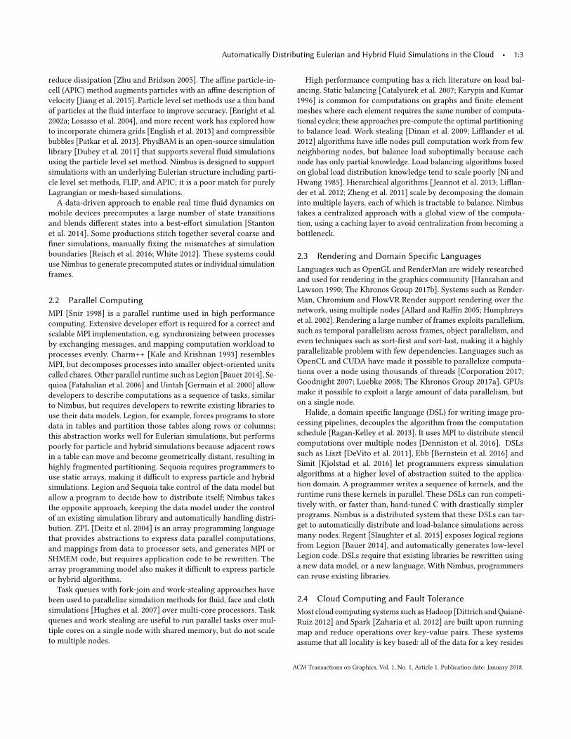
Fig. 1. Particle level set water simulations with and without Nimbus. The left simulation has 1523 cells, runs on a single core and takes 335 minutes to simulate30 frames. The right simulation uses Nimbus to automatically distribute this single-core simulation over 8 nodes (64 cores) in Amazon’s EC2, simulating fasterand with greater detail: 30 frames of a 2563 cell simulation take 268 minutes. Without Nimbus the 2563 cell simulation takes more than two days. Running the1523 simulation in Nimbus takes just over one hour (68 minutes).

Distributing a simulation across many machines can drastically speed upcomputations and increase detail. The computing cloud provides tremendouscomputing resources, but weak service guarantees force programs to managesignificant system complexity: nodes, networks, and storage occasionallyperform poorly or fail.

We describe Nimbus, a system that automatically distributes grid-basedand hybrid simulations across cloud computing nodes. The main simulationloop is sequential code and launches distributed computations across manycores. The simulation on each core runs as if it is stand-alone: Nimbusautomatically stitches these simulations into a single, larger one. To dothis efficiently, Nimbus introduces a four-layer data model that translatesbetween the contiguous, geometric objects used by simulation librariesand the replicated, fine-grained objects managed by its underlying cloudcomputing runtime.

Using PhysBAM particle level set fluid simulations, we demonstrate thatNimbus can run higher detail simulations faster, distribute simulations onup to 512 cores, and run enormous simulations (10243 cells). Nimbus au-tomatically manages these distributed simulations, balancing load acrossnodes and recovering from failures. Implementations of PhysBAM waterand smoke simulations as well as an open source heat-diffusion simulationshow that Nimbus is general and can support complex simulations.

Nimbus can be downloaded from https://nimbus.stanford.edu.

CCS Concepts: •Computingmethodologies→Distributed computingmethodologies; Distributed simulation; Computer graphics;

Permission to make digital or hard copies of part or all of this work for personal orclassroom use is granted without fee provided that copies are not made or distributedfor profit or commercial advantage and that copies bear this notice and the full citationon the first page. Copyrights for third-party components of this work must be honored.For all other uses, contact the owner/author(s).© 2018 Copyright held by the owner/author(s).0730-0301/2018/1-ART1https://doi.org/10.1145/3173551

Additional Key Words and Phrases: Cloud computing, Eulerian and hybridgraphical simulations, load balancing, fault recovery.

ACM Reference format:OmidMashayekhi, Chinmayee Shah, HangQu, Andrew Lim, and Philip Levis.2018. Automatically Distributing Eulerian and Hybrid Fluid Simulations inthe Cloud. ACM Trans. Graph. 1, 1, Article 1 (January 2018), 14 pages.https://doi.org/10.1145/3173551

1 INTRODUCTIONFluid simulation is a cornerstone of modern animation and specialeffects. These simulations are computationally intensive and sotrade off between simulation detail and execution time. Researchresults often run for several days or weeks, but the turn-aroundtimes of production schedules require using lower resolutions.On-demand cloud computing has made high-performance com-

puting clusters immediately available to anyone at very low cost.These ultra-cheap, highly available computing resources are re-sponsible for the success of real-time “big data” analytics frame-works [Murray et al. 2013; Zaharia et al. 2012] as well as a renais-sance in artificial intelligence through deep learning [Dean et al.2012; Lee et al. 2009].Despite its benefits, however, cloud computing has been mostly

untapped by simulations. Writing high-performance, distributedprograms for the cloud is extremely difficult. Cloud computing pro-vides low price points by giving weak service guarantees: nodes,networks, and storage can and do fail quite often [Vishwanath andNagappan 2010]. More perniciously, a small fraction of nodes, calledstragglers, perform poorly [Ananthanarayanan et al. 2010], slowingan application to the speed of the slowest core. To perform well in

ACM Transactions on Graphics, Vol. 1, No. 1, Article 1. Publication date: January 2018.

1:2 • O. Mashayekhi et. al.

the cloud, an application must interleave computation with commu-nication, recover from failures, and dynamically move work awayfrom slow nodes. For one-off simulations, the up-front engineer-ing costs to distribute in the cloud outweigh the benefits. At thesame time, refactoring an existing simulation library is complex anddifficult, requiring deep expertise in both distributed systems andsimulation methods.Existing software frameworks provide little help in writing sim-

ulations for the cloud. Cloud computing frameworks are designedaround application data abstractions such as key-value stores [Mur-ray et al. 2013; Zaharia et al. 2012] or huge graphs [Gonzalez et al.2012; Malewicz et al. 2010], which do not handle the geometricstencils and solvers used by fluid simulations. At the same time,high performance computing (HPC) frameworks leave load balanc-ing and fault tolerance to the programmer (e.g. Charm++ [Kaleand Krishnan 1993]), require rewriting simulation kernels to a re-stricted data model (e.g. X10 [Charles et al. 2005]), or do both (e.g.Legion [Bauer 2014]). Higher level domain specific languages suchas Regent [Slaughter et al. 2015], Simit [Kjolstad et al. 2016], orEbb [Bernstein et al. 2016] require rewriting entire simulations fromscratch and do not provide the load balancing and fault-tolerancethat the cloud requires.This paper presents Nimbus, a system that takes an existing

grid-based or hybrid (e.g., particle level set) simulation library andautomatically distributes it across manymulti-core cloud computingnodes. The core of Nimbus resembles a cloud computing framework:a driver program written as a simple sequential program sendsexecution tasks to a centralized controller node that dispatches themto many worker nodes. Nimbus’s key contribution lies in how itmanages data across compute cores so they each seemingly run astand-alone simulation. Nimbus automatically updates state sharedbetween these sub-simulations (e.g., ghost cells), stitching themtogether into a single larger one. It achieves this by using a novel, 4layer data model:

(1) In the top layer, a sequential driver program executes simu-lation functions over geometric data objects, consisting of asimulation variable over a bounding box.

(2) To efficiently handle ghost regions and other shared subre-gions, the second layer disjointly subdivides the domain intological objects. Logical objects present an abstraction of alarge, shared memory, allowing Nimbus to easily analyzeparallelism and data dependencies independently of how thesimulation is distributed.

(3) Each logical object can have multiple physical instances, re-siding on one or more nodes. The logical/physical separationallows the controller to abstract away distribution, load bal-ancing, and fault tolerance from the driver program.

(4) Finally, application objects are in the format and layout thatthe simulation library expects. Application objects are typ-ically composed of many physical objects, as they includecentral as well as ghost regions. Nimbus automatically up-dates application objects locally or over the network to stitchtogether many seemingly independent simulations.

To support an existing simulation library, a library developerwrites a small number of adapters that translate between librarycalls and Nimbus’s APIs.Nimbus borrows many ideas from previous cloud and HPC sys-

tems, such as a central controller and the distinction between phys-ical and logical objects. Unlike all prior approaches, Nimbus is ableto automatically distribute serial simulations using their existingkernels. Furthermore, running graphical simulations in a cloud com-puting setting exposes new performance bottlenecks that big dataapplications have yet to encounter. Nimbus therefore introducesnew optimization techniques that are crucial for performance, suchas caching translations between physical and application objects aswell as control plane messages. In summary, this paper makes thefollowing contributions:• A four-layer data model that allows a cloud computing run-time to manage distributed geometric data objects that haveoverlapping regions such as ghost cells.• A system architecture that uses the four-layer data modelto automatically distribute a simulation across many cores,stitching together many smaller simulations into a single,larger one.• An evaluation of an implementation of the architecture, calledNimbus, quantifying the overheads and scalability of the un-derlying cloud computing runtime as well as the importanceof data caching enabled by using the four-layer data model.• Demonstrations of PhysBAM [Dubey et al. 2011] particle levelset water and smoke simulations as well as a 3D heat diffusionsimulation using a Jacobi solver that Nimbus automaticallydistributes to run on 1-512 cores.

Our evaluation shows that Nimbus runs more detailed simula-tions faster. By distributing a PhysBAM particle level set watersimulation to run on 64 cores, Nimbus can run a 2563 simulationfaster than a single core can run a 1523 simulation. Alternatively,Nimbus can lower the 1523 simulation time from 4 hours to 1 hour.These improvements come without any modifications to PhysBAMlibraries, demonstrating the benefits of cleanly separating distribu-tion from simulation methods through Nimbus’s system and datamodel. Furthermore, Nimbus is general; in addition to PhysBAMwater and smoke simulations, we demonstrate a 3D heat diffusionsimulation [Kamil 2017] distributed by Nimbus.

2 RELATED WORKThis work builds upon and borrows ideas from a diverse body ofprior work including fluid simulation methods, parallel computing,DSLs, and cloud computing.

2.1 Fluid SimulationsThere are several common techniques used in fluid simulations.Some, such as smoothed-particle hydrodynamics (SPH) [Desbrunand Gascuel 1996], are purely particle-based (Lagrangian). Othersare purely grid-based (Eulerian) [Stam 1999]. Most modern methods,however, use a combination of particles and grids. The particle-in-cell (PIC) method uses a grid for pressure and viscosity updatesbut particles for advection [Harlow 1962]. The fluid implicit par-ticle method (FLIP) adds energy and momentum to particles to


Automatically Distributing Eulerian and Hybrid Fluid Simulations in the Cloud • 1:3

reduce dissipation [Zhu and Bridson 2005]. The affine particle-in-cell (APIC) method augments particles with an affine description ofvelocity [Jiang et al. 2015]. Particle level set methods use a thin bandof particles at the fluid interface to improve accuracy. [Enright et al.2002a; Losasso et al. 2004], and more recent work has explored howto incorporate chimera grids [English et al. 2013] and compressiblebubbles [Patkar et al. 2013]. PhysBAM is an open-source simulationlibrary [Dubey et al. 2011] that supports several fluid simulationsusing the particle level set method. Nimbus is designed to supportsimulations with an underlying Eulerian structure including parti-cle level set methods, FLIP, and APIC; it is a poor match for purelyLagrangian or mesh-based simulations.A data-driven approach to enable real time fluid dynamics on

mobile devices precomputes a large number of state transitionsand blends different states into a best-effort simulation [Stantonet al. 2014]. Some productions stitch together several coarse andfiner simulations, manually fixing the mismatches at simulationboundaries [Reisch et al. 2016; White 2012]. These systems coulduse Nimbus to generate precomputed states or individual simulationframes.

2.2 Parallel ComputingMPI [Snir 1998] is a parallel runtime used in high performancecomputing. Extensive developer effort is required for a correct andscalable MPI implementation, e.g. synchronizing between processesby exchanging messages, and mapping computation workload toprocesses evenly. Charm++ [Kale and Krishnan 1993] resemblesMPI, but decomposes processes into smaller object-oriented unitscalled chares. Other parallel runtime such as Legion [Bauer 2014], Se-quioa [Fatahalian et al. 2006] and Uintah [Germain et al. 2000] allowdevelopers to describe computations as a sequence of tasks, similarto Nimbus, but requires developers to rewrite existing libraries touse their data models. Legion, for example, forces programs to storedata in tables and partition those tables along rows or columns;this abstraction works well for Eulerian simulations, but performspoorly for particle and hybrid simulations because adjacent rowsin a table can move and become geometrically distant, resulting inhighly fragmented partitioning. Sequoia requires programmers touse static arrays, making it difficult to express particle and hybridsimulations. Legion and Sequoia take control of the data model butallow a program to decide how to distribute itself; Nimbus takesthe opposite approach, keeping the data model under the controlof an existing simulation library and automatically handling distri-bution. ZPL [Deitz et al. 2004] is an array programming languagethat provides abstractions to express data parallel computations,and mappings from data to processor sets, and generates MPI orSHMEM code, but requires application code to be rewritten. Thearray programming model also makes it difficult to express particleor hybrid algorithms.Task queues with fork-join and work-stealing approaches have

been used to parallelize simulation methods for fluid, face and clothsimulations [Hughes et al. 2007] over multi-core processors. Taskqueues and work stealing are useful to run parallel tasks over mul-tiple cores on a single node with shared memory, but do not scaleto multiple nodes.

High performance computing has a rich literature on load bal-ancing. Static balancing [Catalyurek et al. 2007; Karypis and Kumar1996] is common for computations on graphs and finite elementmeshes where each element requires the same number of computa-tional cycles; these approaches pre-compute the optimal partitioningto balance load. Work stealing [Dinan et al. 2009; Lifflander et al.2012] algorithms have idle nodes pull computation work from fewneighboring nodes, but balance load suboptimally because eachnode has only partial knowledge. Load balancing algorithms basedon global load distribution knowledge tend to scale poorly [Ni andHwang 1985]. Hierarchical algorithms [Jeannot et al. 2013; Lifflan-der et al. 2012; Zheng et al. 2011] scale by decomposing the domaininto multiple layers, each of which is tractable to balance. Nimbustakes a centralized approach with a global view of the computa-tion, using a caching layer to avoid centralization from becoming abottleneck.

2.3 Rendering and Domain Specific LanguagesLanguages such as OpenGL and RenderMan are widely researchedand used for rendering in the graphics community [Hanrahan andLawson 1990; The Khronos Group 2017b]. Systems such as Render-Man, Chromium and FlowVR Render support rendering over thenetwork, using multiple nodes [Allard and Raffin 2005; Humphreyset al. 2002]. Rendering a large number of frames exploits parallelism,such as temporal parallelism across frames, object parallelism, andeven techniques such as sort-first and sort-last, making it a highlyparallelizable problem with few dependencies. Languages such asOpenCL and CUDA have made it possible to parallelize computa-tions over a node using thousands of threads [Corporation 2017;Goodnight 2007; Luebke 2008; The Khronos Group 2017a]. GPUsmake it possible to exploit a large amount of data parallelism, buton a single node.Halide, a domain specific language (DSL) for writing image pro-

cessing pipelines, decouples the algorithm from the computationschedule [Ragan-Kelley et al. 2013]. It uses MPI to distribute stencilcomputations over multiple nodes [Denniston et al. 2016]. DSLssuch as Liszt [DeVito et al. 2011], Ebb [Bernstein et al. 2016] andSimit [Kjolstad et al. 2016] let programmers express simulationalgorithms at a higher level of abstraction suited to the applica-tion domain. A programmer writes a sequence of kernels, and theruntime runs these kernels in parallel. These DSLs can run competi-tively with, or faster than, hand-tuned C with drastically simplerprograms. Nimbus is a distributed system that these DSLs can tar-get to automatically distribute and load-balance simulations acrossmany nodes. Regent [Slaughter et al. 2015] exposes logical regionsfrom Legion [Bauer 2014], and automatically generates low-levelLegion code. DSLs require that existing libraries be rewritten usinga new data model, or a new language. With Nimbus, programmerscan reuse existing libraries.

2.4 Cloud Computing and Fault ToleranceMost cloud computing systems such asHadoop [Dittrich andQuiané-Ruiz 2012] and Spark [Zaharia et al. 2012] are built upon runningmap and reduce operations over key-value pairs. These systemsassume that all locality is key based: all of the data for a key resides



BA C D

Ghost Regions

21 3 4 5 6

Geometric(driver)

Logical

Application(library)

Physical

ReadWrite

WriteRead

Data Type

Node 1 Node 2

Launcher

Controller

Translator

Fig. 2. The Nimbus data model has four abstractions: geometric, logical,physical, and application. This example shows a 1D advection stencil splitinto two partitions on two different nodes. The geometric view sees thecomplete simulation domain and applies the stencil to the two partitions.This defines 4 logical objects, which map to 6 physical objects on the twonodes. Nimbus assembles these disjoint physical objects into contiguousapplication objects before invoking simulation library functions.

on the same node, but data for different keys has no locality. Corre-spondingly, these systems support when a task either depends on asingle partition (a “narrow” dependency) or all partitions (a “wide”dependency) of data, but nothing in-between. This abstraction ispoorly suited to the structure and locality of simulation data suchas particles and grids. Nimbus extends this task based approach tosupport geometric dependencies with data locality.Cloud nodes can have highly variable performance, due to net-

work cross-traffic, misconfiguration, or hardware faults. This causesa small fraction of nodes to be “stragglers”. Cloud systems ad-dress stragglers and failures by proactively replicating computa-tions [Ananthanarayanan et al. 2013; Dean and Ghemawat 2008],which works well for disk bound computations but is prohibitivelyexpensive for CPU-bound ones. Spark tracks lineage for each dataset, recomputing and regenerating them if needed.

Naiad uses a timely dataflow to track dependencies, and supportsricher programs such as streaming data analysis, machine learningand graph mining [Murray et al. 2013]. TensorFlow automaticallydistributes machine learning algorithms, expressed as a dataflowgraph of mathematical operations (nodes) and multi-dimensionalarrays or tensors (edges) [Abadi et al. 2016]. Nimbus borrows theideas of expressing dependencies using a dataflow graph and usinga controller to place data and schedule tasks, from these systems.Nimbus provides a richer API to express simulation data such asparticles and grids, and simulation algorithms and solvers.When the mean number of failures or time between failures is

known, approximations such as Young’s formula [Di et al. 2013;Young 1974] can be used to compute the optimal number of check-points. Systems such as Berkeley Lab Checkpoint/Restart (BLCR) [Har-grove and Duell 2006] and Distributed Multi-threaded Checkpoint-ing (DMTCP) [Ansel et al. 2009] provide mechanisms and toolsto checkpoint processes and restart processes from checkpoints,which libraries and applications can use to recover from faults.However, these systems do not migrate ongoing computations forload-balancing, and require users to correctly distribute code, syn-chronize execution, and exchange messages between processes.

3 FOUR LAYER DATA MODELNimbus automatically stitches together distributed, sequential, stand-alone simulations into a single, larger simulation. It accomplishesthis by using a powerful four-layer data model tailored to the re-sponsibilities of four different program representations, shown inFigure 2. These four layers of abstraction provide a clear separationof concerns for different parts of the system, distributing manage-ment of the computation in an efficient manner while hiding thedetails of parallelism, distribution, and fault recovery from the pro-grammer.The geometric layer is designed to provide a simple abstraction

to a simulation author. It is written as a sequential program andcompletely hides how data is partitioned and computations aredistributed. The logical layer breaks this geometry into disjoint dataobjects and is designed to allow the cloud runtime to quickly analyzedependencies as well as how to place and replicate data. The physicallayer maps the logical objects to specific memory on workers and isdesigned to allow the distributed worker nodes to replicate objectsas well as synchronize them. Finally, the application layer is designedto allow existing simulation kernels to use their own custom datastructures and data representations without modification.

Figure 2 shows the three software systems that manage the inter-faces between these layers. Section 4 discusses these in detail, butthe translator is notable because it motivates the need for a 4-layerdata model. The translator performs the critical conversion betweenphysical objects and the application object formats that a simulationlibrary expects. The translator is critical for performance because asingle application object often consists of many physical objects. Forexample, node 1’s application object in Figure 2 consists of objects 1,2, and 3. The application expects its object to be a contiguous blockof memory to make memory accesses fast, but the worker needs tostore it as three separate blocks of memory to make memory andnetwork transfers fast.The rest of this section explains the four data abstractions in

greater detail. Section 4 describes how Nimbus uses each one andtranslates between them.

3.1 GeometricA simulation declares a variable as a data type over the simulationdomain with a geometric partitioning and a ghost cell width. Thesimulation library defines the set of available types, such as floatingpoint vectors, particles, or scalars. The simulation loop is a linearsequence of simulation library calls, such as advecting particlesor calculating boundary conditions in projection. Each library callspecifies its data reads and writes by a set of {variable, bounding box}pairs. The 1D stencil in Figure 2, for example, makes two librarycalls, one on the left bounding boxes and one on the right:

parallel {apply(advect, {vel, lread_bb}, {vel, lwrite_bb});apply(advect, {vel, rread_bb}, {vel, rwrite_bb});

}

Different simulation variables may have different partitioning. Forexample, aMAC grid can use a fine-grained partitioning tomaximizeparallelism while a matrix used during a solve can be partitioned



more coarsely to reduce the number of iterations needed to con-verge.

3.2 LogicalUsing the specified partitioning, Nimbus’s launcher automaticallytranslates each variable’s geometric domain into a set of disjoint log-ical objects. Logical objects present the abstraction of a single large,shared memory. They expose how a simulation can be parallelizedbut hide how the simulation is distributed. Automatically paralleliz-ing a sequential simulation requires carefully managing the readand write order of variables to ensure that a lightly loaded workerdoes not race ahead and read input data before prior operations onother nodes have completed.Logical objects define a read/write order to enforce that the par-

allelized, distributed simulation behaves like the sequential driverprogram. Each object has a linear sequence of writes, with any num-ber of parallel reads between a pair of writes. This allows Nimbusto analyze data dependencies between calls and enforce executionorder. Figure 2 has four logical objects. Nimbus transforms the twolibrary calls into:parallel {

apply(advect, read:{A, B, C}, write:{A, B});apply(advect, read:{B, C, D}, write:{C, D});

}

As these two advection calls are in parallel, Nimbus knows thatboth of them read the same data in B and C and they can execute inparallel. However, the next time this block executes, each advectioncall reads the output of the prior calls and so cannot run until theprior invocations complete. Nimbus allows in-place operations onregions that have read-write access permissions. However, parallelwrites to a region are not allowed. In simulation steps where ghostregions have parallel writes (e.g., particle advection), Nimbus uses atwo stage operation, first creating one temporary object per writerand then reducing them to the final result.

3.3 PhysicalEach logical object has one or more associated physical objects. Aphysical object describes actual simulation state stored in the mem-ory of a specific node. Physical objects therefore define how dataand computations are distributed. Operations on physical objectsdescribe the simulation’s execution as managed by the cloud run-time, including simulation operations and data movement. Nimbus’scontroller binds references to logical objects to concrete physicalinstances as it decides how to distribute the simulation.When distributed across two nodes, the 4 logical objects in Fig-

ure 2 map to 6 physical objects, 3 on each node ({1,2,3} and {4,5,6}).The logical library calls above are translated into these physicallibrary calls:

apply(advect, read:{1, 2, 3}, write:{1, 2});apply(advect, read:{4, 5, 6}, write:{5, 6});

and before any future operations that require accessing updatedghost regions, Nimbus synchronizes ghost objects through explicitphysical copy calls:

network_copy(from:2, to:4);network_copy(from:5, to:3);

Unlike the logical view of objects, which maintain the abstractionof a sequential execution of parallel operators, the physical viewdescribes their actual execution. It presents a level of abstractionthat allows workers to intelligently and correctly manage executionwhile remaining independent of the simulation library they areusing.Physical objects are stored as contiguous blocks of memory, op-

timized for network transfer and minimizing fragmentation. Sec-tion 4.2 describes how Nimbus copies physical objects to ensurethat, when it executes, each library call reads the result of the mostrecent write to an object.

3.4 ApplicationNimbus’s runtime needs to pass properly formatted data to a li-brary’s simulation kernels. When Nimbus invokes a kernel, it doesso as if a partition of the larger simulation is itself a stand-alone,smaller simulation. Ghost cells and other replicated subsets of thedata are hidden from the library: a single application object typicallyconsists of many physical objects. The simulation library, however,often assumes that the application object is a single, contiguousobject in memory. For example, iterating across the application datafor Node 1 in Figure 2 requires accessing object 1, then object 2,then object 3.

Nimbus’s translator assembles application objects by interleavingdata from physical objects. Nimbus uses the geometry metadata ofthe physical objects to interleave them correctly. Simulation libraryfunctions over these application objects can be used unmodified,without rewriting code to use a different data model. Figure 2 showshow the two nodes each assemble a contiguous application-levelobject out of 3 disjoint physical objects. For example, a PhysBAMapplication object can refer to scalar or vector arrays, or particlesstored as an array of linked lists of buckets of particles.

advect(sim.velocity());

As the call above shows, the simulation library executing onthe node is unaware that its application object can be modifiedby other threads, cores, or nodes. Instead, when a library routinecompletes, Nimbus automatically updates the underlying physicalobjects, stitching together the seemingly independent simulations.The controller automatically copies the physical object that containsthe latest writes to a logical object to other physical objects. BeforeNimbus runs a simulation kernel on application objects, it checkswhether they are up to date with their corresponding physical ob-jects. If the physical objects have updates, Nimbus merges thoseupdates into the application object before running the kernel. Forexample, when node 2 copies 5 to 3, the next time node 1 runs thekernel it merges the writes to 3 into the corresponding applicationobject. Section 4.3 describes how the translator automatically keepsapplication layer data objects and their underlying physical objectsconsistent.

4 SYSTEM DESIGNThis section presents how Nimbus’s seemingly complex servicescan be decomposed into a few simple system components. Nim-bus translates between geometric, logical, physical, and applicationviews of the data using the five architecture components shown in



Driver Program:

Partition prt = {2, 1, 1};Create(velocity, prt);

Op(exec: advect, data: velocity, read: core/ghost, write: ghost);

...Laun

cher

PhysicalData

Mappings

Controller

BA C D

21 34 5 6

LogicalDataCopyTasks

TranslatorManager

app.so

21 3

TranslatorManager

4 5 6

app.so

PhysicalTask(advect, {1,2,3})

PhysicalTask(advect, {4,5,6})LogicalTask(advect, {A,B,C})LogicalTask(advect, {B,C,D})

WorkerNodes

GeometricTask(advect, left_reg)GeometricTask(advect, right_reg)

ApplicaDonData

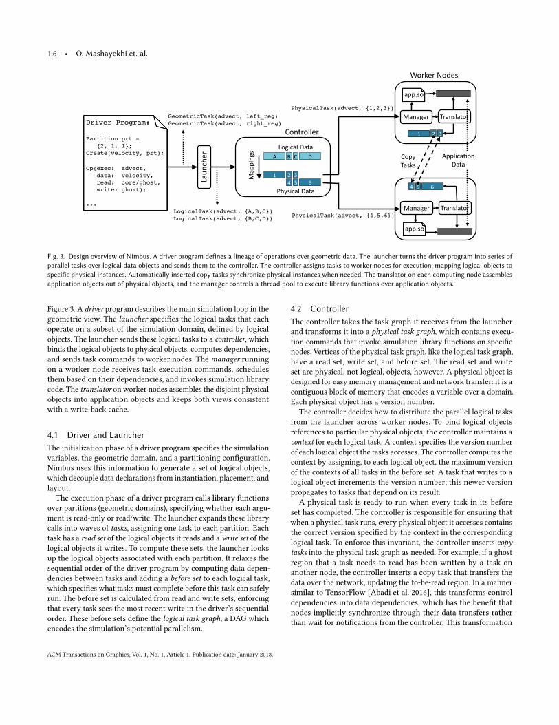
Fig. 3. Design overview of Nimbus. A driver program defines a lineage of operations over geometric data. The launcher turns the driver program into series ofparallel tasks over logical data objects and sends them to the controller. The controller assigns tasks to worker nodes for execution, mapping logical objects tospecific physical instances. Automatically inserted copy tasks synchronize physical instances when needed. The translator on each computing node assemblesapplication objects out of physical objects, and the manager controls a thread pool to execute library functions over application objects.

Figure 3. A driver program describes the main simulation loop in thegeometric view. The launcher specifies the logical tasks that eachoperate on a subset of the simulation domain, defined by logicalobjects. The launcher sends these logical tasks to a controller, whichbinds the logical objects to physical objects, computes dependencies,and sends task commands to worker nodes. The manager runningon a worker node receives task execution commands, schedulesthem based on their dependencies, and invokes simulation librarycode. The translator on worker nodes assembles the disjoint physicalobjects into application objects and keeps both views consistentwith a write-back cache.

4.1 Driver and LauncherThe initialization phase of a driver program specifies the simulationvariables, the geometric domain, and a partitioning configuration.Nimbus uses this information to generate a set of logical objects,which decouple data declarations from instantiation, placement, andlayout.The execution phase of a driver program calls library functions

over partitions (geometric domains), specifying whether each argu-ment is read-only or read/write. The launcher expands these librarycalls into waves of tasks, assigning one task to each partition. Eachtask has a read set of the logical objects it reads and a write set of thelogical objects it writes. To compute these sets, the launcher looksup the logical objects associated with each partition. It relaxes thesequential order of the driver program by computing data depen-dencies between tasks and adding a before set to each logical task,which specifies what tasks must complete before this task can safelyrun. The before set is calculated from read and write sets, enforcingthat every task sees the most recent write in the driver’s sequentialorder. These before sets define the logical task graph, a DAG whichencodes the simulation’s potential parallelism.

4.2 ControllerThe controller takes the task graph it receives from the launcherand transforms it into a physical task graph, which contains execu-tion commands that invoke simulation library functions on specificnodes. Vertices of the physical task graph, like the logical task graph,have a read set, write set, and before set. The read set and writeset are physical, not logical, objects, however. A physical object isdesigned for easy memory management and network transfer: it is acontiguous block of memory that encodes a variable over a domain.Each physical object has a version number.

The controller decides how to distribute the parallel logical tasksfrom the launcher across worker nodes. To bind logical objectsreferences to particular physical objects, the controller maintains acontext for each logical task. A context specifies the version numberof each logical object the tasks accesses. The controller computes thecontext by assigning, to each logical object, the maximum versionof the contexts of all tasks in the before set. A task that writes to alogical object increments the version number; this newer versionpropagates to tasks that depend on its result.A physical task is ready to run when every task in its before

set has completed. The controller is responsible for ensuring thatwhen a physical task runs, every physical object it accesses containsthe correct version specified by the context in the correspondinglogical task. To enforce this invariant, the controller inserts copytasks into the physical task graph as needed. For example, if a ghostregion that a task needs to read has been written by a task onanother node, the controller inserts a copy task that transfers thedata over the network, updating the to-be-read region. In a mannersimilar to TensorFlow [Abadi et al. 2016], this transforms controldependencies into data dependencies, which has the benefit thatnodes implicitly synchronize through their data transfers ratherthan wait for notifications from the controller. This transformation



ensures that the controller does not become a bottleneck at moderatescales, a problem noted by Sparrow [Ousterhout et al. 2013]. Copytasks can be local or remote. Local copy tasks copy between twomemory buffers. Remote copy tasks perform a network transferusing asynchronous I/O. Each computational node has a single I/Othread that handles completion events and updates the physicalgraph.When deciding how many physical instances to create, the con-

troller trades off between memory footprint and parallelism with asimple heuristic. It makes multiple instances of ghost regions butkeeps a single instance of any central region. For the uniform parti-tioning of 2563 simulation in Figure 1, for example, a 3-wide ghostregion has has 9 to 10,092 cells1, while a central region has 195,112cells. Section 6 describes how the controller decides where to placephysical objects.

4.2.1 Controller Cache. For large, distributed simulations withhundreds of partitions and millions of logical and physical objects,computing and sending logical tasks to the controller and mappinglogical tasks to physical tasks can become a bottleneck. Since simula-tions involve iterative loops with regular access patterns, they haveboth regular control flow and data flow. The launcher and controllertherefore cache the tasks they generate, similarly to how executiontemplates can improve data analytics scalability [Mashayekhi et al.2017]. Cache misses only occur the first time a control path executes(e.g., the first iteration, the first time a frame is written to disk, etc.).On subsequent executions, rather than compute and send thousandsof tasks, the controller and workers have cached copies of entire tasksubgraphs, which can be invoked with a single network message; acache hit allows a single message to schedule tens of thousands oflow latency tasks.

4.3 Manager and TranslatorThe manager receives tasks from the controller and manages threetask queues: blocked (on an incomplete member of the before set),ready, and running. It maintains a subset of the physical task graph,consisting of the tasks received from the controller. When a taskcompletes, the manager removes it from all task before sets; if thismakes a before set of a task empty, that task transitions to the readyqueue. The manager maintains a thread pool equal to the number ofavailable cores. When a task completes, it takes the next task of theready queue and runs it. The ready queue uses two priorities, witheach priority having a FIFO order. Copy tasks have higher priority.This starts asynchronous network transfers as early as possible,interleaving communication and computation.Before the manager executes a simulation library function, it

invokes the translator to generate the appropriate application objects.If there is already an application object whose data has the correctversions, the translator returns immediately. If there are portions ofthe object that do not contain the most recent write (e.g., a ghostregion written to by another node), it fills into the application objectthe contents of the physical object specified in the task.

4.3.1 Translator Cache. To prevent unnecessary copies for datathat is only used locally, and to remove the need for two copies

1 The largest ghost region has 3 × (256/4 − 2 × 3)2 = 10, 092 cells.

of central regions, the translator uses a write-back cache. If a taskwrites to an application object, the translator does not immediatelywrite out the result to the corresponding physical objects. Instead,it waits until a copy task reads the physical object, at which point itwrites the result out to the physical object before the transfer starts.The translator frees the backing memory of physical objects thatare out of date with their application object. Because central regionsare only transferred when Nimbus load balances between workernodes, there is only one copy of their data. This allows Nimbus tomaintain both the system and application views with only a small(< 10%) memory overhead.

5 WRITING SIMULATIONS WITH NIMBUSWriting a simulation in Nimbus has two parts. First, a simulationlibrary developer writes adapters that allow Nimbus to translatebetween the application and system views, and compute tasks thatencapsulate library function calls. This is a one-time effort. Second,the simulation author writes the driver program that specifies thevariables and computational steps of a specific simulation withcontrol tasks.

This section explains Nimbus’s API, using level set advection asa running example. The application simulates multiple frames, andassumes one iteration per frame for simplicity (PhysBAM dynami-cally selects a dt inversely proportional to the maximum velocityin order to maintain the CFL condition). It explains both the APIsused for adapters as well as a simulation driver.

5.1 Simulation Types (Library Developer)For Nimbus to translate between the application and system views, asimulation library developer has to write an adapter for the transla-tor to convert them. This adapter is a class that holds the underlyingapplication data. Listing 1 illustrates this API for a scalar array inPhysBAM (e.g., the signed distance). The Read method reads out ofthe application object, translating it into physical objects. The boxparameter specifies a bounding box subset of the application objectto copy. Each element of objects also has a bounding box; the datacopied is the intersection of the application object bounding box, thephysical object bounding box, and box. Write copies from physicalobjects into the application object.

5.2 Compute Tasks (Library Developer)For Nimbus to be able to invoke simulation kernels through tasks,simulation library developers must write adapters between the Nim-bus APIs and each kernel. Compute tasks encapsulate calls intosimulation library function. They are responsible for setting anyglobal variables or configuration that the simulation library expects.They also fetch the application objects from the translator that thesimulation library function needs. Compute task logic determineswhen boundary conditions are used (e.g., compute tasks take a dif-ferent branch if a cell is a boundary). Listing 2 shows simplifiedcode for the AdvectLevelset compute task. The compute task readsvelocity and signed_distance over its partition and ghost regionsfrom neighboring partitions, advects signed_distance with a call toPhysBAMAdvectLevelset, and writes to signed_distance in its parti-tion.



1 class ScalarArray: public AppVar {

2 PhysBAMScalarArray *data ();

3 void Read(DataArray objects, BBox box);

4 void Write(DataArray objects, BBox box);

5 // Internal data members

6 Region bounding_box;

7 PhysBAMScalarArray *data;

8 };

Listing 1. Type definition for a float array application object.

1 class AdvectLevelset: public ComputeTask {

2 void Execute() {

3 // Get application objects to compute on

4 float& dt = GetAppObject("dt");

5 Vec3fArray& vel = GetAppObject("velocity");

6 FloatArray& sdist =

7 GetAppObject("signed_distance");

8 // Call into the PhysBAM library

9 PhysBAMAdvectLevelset(

10 vel.data(), sdist.data(), dt);

11 }

12 };

Listing 2. Compute task for advecting level set calls into PhysBAM.

5.3 Driver Program (Simulation Author)The driver program has three parts, shown in Listings 3–5. The firstpart (Listing 3) defines the parameters of the simulation, includingthe geometric domain, partitioning, and ghost cell widths. Thisinitialization is the one point in the program when a simulationauthor must consider how to distribute the simulation. Unlike HPCsimulations, which tend to perform a uniform computation overdata, graphical simulations can have highly varying computations.For example, particle level set water simulations perform far morecomputations on water cells than air cells, and water cells on theinterface are more computationally intensive than those deep withinthe volume. As a result, the optimal partitioning depends not onlyon the type of simulation, but also its initial conditions, and so thisis best controlled by the simulation author.

The driver program is written as a control task. Control tasks donot directly invoke simulation functions; instead, they launch othercompute and control tasks. A special control task, Main (Listing 4), isthe entry point for simulation. Main defines the simulation variables.These variable definitions create logical objects at the controller.The controller does not create physical objects on worker nodesuntil it sends tasks to read or write them. This lazy instantiationallows the controller to distribute data only after it has a full pictureof task access patterns on data objects.

Main, after it launches tasks to initialize the simulation, launches aLoop task, which corresponds to the outermost simulation loop. Thistask launches compute tasks AdvectLevelset and AdvectVelocity

(Listing 5) to compute the next values of signed_distance and

1 // Define simulation domain

2 BondingBox sim_region = {{0,0,0},{256,256,256}};

3 // Partition the domain along three axes

4 Partitioning partitioning = {2,2,1};

5 // The width of the ghost region

6 int ghost_width = 2;

7 // Center regions with ghost width 0

8 Region center({sim_region, partitioning, 0});

9 // Outer regions includes center and ghost regions

10 Region outer({sim_region, partitioning, ghost_width});

Listing 3. Example initialization of a 2563 simulation domain partitioned inhalf along the X and Y axes.

1 // Entry point for a simulation

2 class Main: public ControlTask {

3 void Execute() {

4 CreateData("signed_distance", FloatArray, sim_region,

5 ghost_width, partitioning);

6 CreateData("velocity", Vec3fArray, sim_region,

7 ghost_width, partitioning);

8 // Create more objects and launch Loop task

9 }

10 };

Listing 4. Main task for example particle level set simulation.

1 // A control task to loop until target_frame

2 class Loop: public ControlTask {

3 void Execute() {

4 // Spawn parallel AdvectLevelset tasks

5 LaunchTaskOverAllPartitions(

6 AdvectLevelset,

7 {{"signed_distance", outer},

8 {"velocity", outer}}, // Read outer

9 {{"signed_distance", center}}, // Write center

10 {}); // No task parameter

11 // Spawn other tasks to advect velocity

12 // Spawn next iteration if needed

13 if (parameter.current_frame < parameter.target_frame)

14 LaunchTask(

15 Loop, {}, {} // No read/write data

16 { .current_frame = parameter.current_frame + 1,

17 .target_frame = parameter.target_frame });

18 }

19 };

Listing 5. Loop task for example particle level set simulation.

velocity. Loop task uses parameters current_frame and target_frameto determine the end of simulation, or launches another Loop controltask.When launching compute tasks, a control task must specify the

data that the compute task reads and writes, plus optional task spe-cific parameters. For instance, the Loop task specifies read and writesets for AdvectLevelset on lines 5 to 10. It does this by specifying



the variables and the partitioning to use for reading and writing –an AdvectLevelset task over a partition writes to signed_distance

only over the same partition, by specifying center as the partition towrite, but reads signed_distance and velocity from ghost regionsover neighboring partitions. Nimbus automatically infers write af-ter read dependencies (e.g., from AdvectLevelset to AdvectVelocity),and read after write dependencies (from AdvectVelocity to AdvectLevelset). Based on these dependencies, it automatically inserts the neces-sary copy tasks and adds them to before sets, enforcing the correctexecution order.

6 FAULT TOLERANCE AND LOAD BALANCINGProduction simulations over large grids require hundreds of GB ofmemory and thousands of hours of CPU cycles. Simulations runningin the cloud must deal with straggler nodes, arising from oversub-scribed and shared resources such as worker nodes and networkcapacity, and failures such as I/O failures. Private clusters also ex-hibit these problems when using a large number of nodes for longperiods of time. Disruptions due to failures and slow-down dueto straggler nodes can be very expensive in terms of time and ef-fort. Nimbus automatically load-balances applications, and recoversapplications from failures (provides fault tolerance).

6.1 Fault ToleranceThe Nimbus controller periodically saves a snapshot of applicationstate and data, allowing it to restart a simulation in case of a failure.These checkpoints are sharded over worker nodes and indexed by adistributed key-value store on top of leveldb [Ghemawat and Dean2017]. At every checkpoint, Nimbus saves the current task graph,which includes all control and compute tasks, and system data ob-jects. Worker nodes periodically send a heartbeat message to thecontroller. When the controller does not see heartbeat messagesfrom a worker, it assumes that the node has failed. When a node fails,the controller resets the state to the most recent checkpoint, reas-signs partitions and tasks across the remaining nodes, and resumesthe simulation.

6.2 Load BalancingNimbus worker nodes periodically send total time spent in computa-tion tasks to the controller. A high compute time to total time ratioindicates that a node may be a straggler – the node takes more timeto complete compute tasks, while other nodes are blocked on it forupdated ghost data. Such imbalance can come from oversubscrip-tion of shared resources or interference from other applications,difference in CPU speeds, or even from within the application, forinstance, due to varying amount of fluid. For instance, a particle levelset fluid simulation may have more computation near the interface,due to additional particles. Most fluid simulations, such as particlelevel set, FLIP and APIC have different amounts of fluid in differentpartitions, as the simulated fluid evolves over time. This results invariation across partitions and time. A low compute time to totaltime ratio triggers migration – Nimbus moves some partitions fromthe straggling worker to neighboring workers. The controller sendscommands to migrate tasks and data to worker nodes, and workernodes exchange data accordingly. This is repeated until the ratio of

2 8 16 32 48 64Number of workers

0

20

40

60

Speedup v

s. s

ingle

work

er

63.8x

19.2x15.2x

8.2x

ghost bw: 0

ghost bw: 1

ghost bw: 2

ghost bw: 3

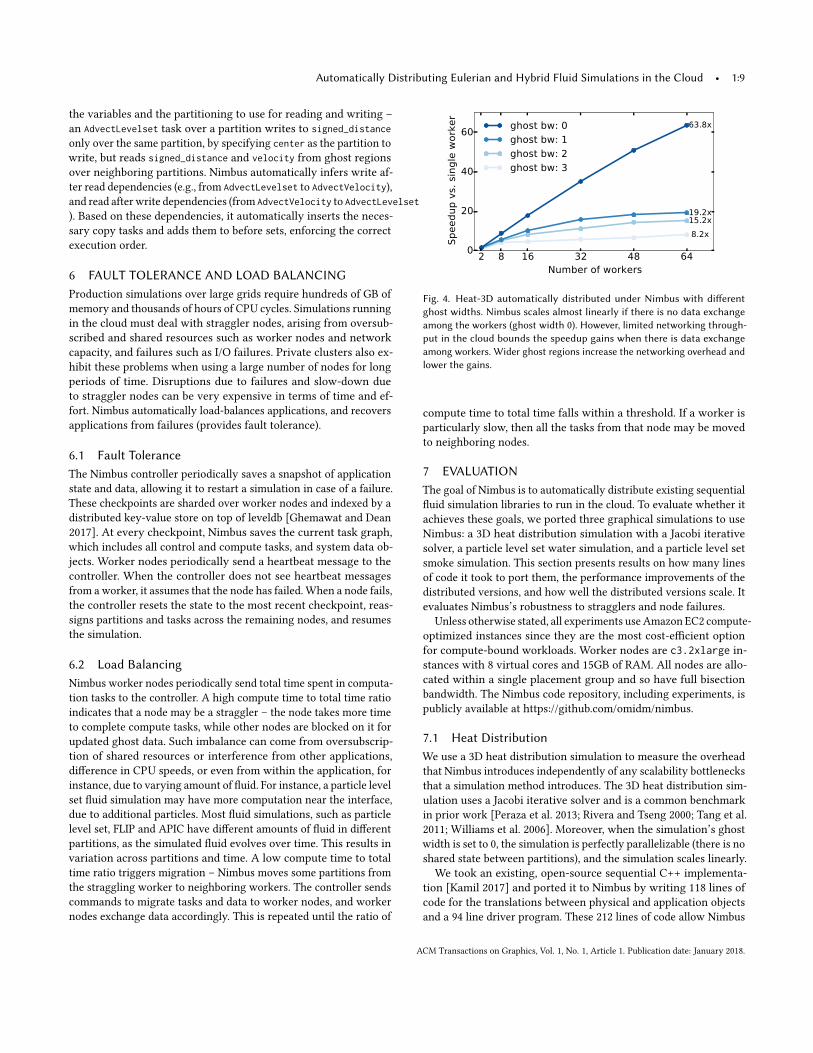
Fig. 4. Heat-3D automatically distributed under Nimbus with differentghost widths. Nimbus scales almost linearly if there is no data exchangeamong the workers (ghost width 0). However, limited networking through-put in the cloud bounds the speedup gains when there is data exchangeamong workers. Wider ghost regions increase the networking overhead andlower the gains.

compute time to total time falls within a threshold. If a worker isparticularly slow, then all the tasks from that node may be movedto neighboring nodes.

7 EVALUATIONThe goal of Nimbus is to automatically distribute existing sequentialfluid simulation libraries to run in the cloud. To evaluate whether itachieves these goals, we ported three graphical simulations to useNimbus: a 3D heat distribution simulation with a Jacobi iterativesolver, a particle level set water simulation, and a particle level setsmoke simulation. This section presents results on how many linesof code it took to port them, the performance improvements of thedistributed versions, and how well the distributed versions scale. Itevaluates Nimbus’s robustness to stragglers and node failures.

Unless otherwise stated, all experiments use Amazon EC2 compute-optimized instances since they are the most cost-efficient optionfor compute-bound workloads. Worker nodes are c3.2xlarge in-stances with 8 virtual cores and 15GB of RAM. All nodes are allo-cated within a single placement group and so have full bisectionbandwidth. The Nimbus code repository, including experiments, ispublicly available at https://github.com/omidm/nimbus.

7.1 Heat DistributionWe use a 3D heat distribution simulation to measure the overheadthat Nimbus introduces independently of any scalability bottlenecksthat a simulation method introduces. The 3D heat distribution sim-ulation uses a Jacobi iterative solver and is a common benchmarkin prior work [Peraza et al. 2013; Rivera and Tseng 2000; Tang et al.2011; Williams et al. 2006]. Moreover, when the simulation’s ghostwidth is set to 0, the simulation is perfectly parallelizable (there is noshared state between partitions), and the simulation scales linearly.We took an existing, open-source sequential C++ implementa-

tion [Kamil 2017] and ported it to Nimbus by writing 118 lines ofcode for the translations between physical and application objectsand a 94 line driver program. These 212 lines of code allow Nimbus



2 8 16 32 48 64Number of workers

0

10

20

30

Speedup v

s. s

ingle

work

er

19.2x

11.1x

1.0x

w/ translator and controller cache

w/ only controller cache

w/ only translator cache

no caching

Fig. 5. Effect of translator and controller caches on scalability of the Heat-3D application under Nimbus with a ghost width of 1. The translator andcontroller caches are crucial for Nimbus’s scalability. Without the translatorcache the applications run almost two times slower. Without the controllercache, the controller becomes a bottleneck at even moderate scales andlimits the performance gains from scaling.

to automatically stitch together many distributed sub-simulationsinto a single, large simulation.

7.1.1 Scalability. Figure 4 shows the speedup gains from usingNimbus to distribute the 3D heat distribution simulation over 2–64workers. When the ghost width is 0, each sub-simulation runs inde-pendently. With 64 workers, the simulation runs 63.8x times fasterthan on a single worker: Nimbus’s overhead is < 0.4%. Increasingthe ghost width introduces data exchanges between sub-simulations.Because c3.2x large instances have only 1Gbps links, these dataexchanges become a bottleneck; the simulation method limits scala-bility. Using a ghost width of 3 cells, 64 worker nodes speed up thesimulation by 8.2x. We verified that communication is the bottle-neck by using a distributed logging mechanism similar to block-timeanalysis [Ousterhout et al. 2015].

7.1.2 Translator and Controller Cache. Nimbus’s translator andcontroller caches are designed to address performance bottlenecksthat graphical simulations introduce but traditional cloud systems donot encounter. To quantify the performance benefits of the translatorand controller caches, we ran simulations with a ghost cell size of 1,as this is the fastest setting that exercises the translator cache.Figure 5 shows the results. The translator cache improves per-

formance by 72%. Without a translator cache, Nimbus is forced totranslate central regions back and forth between the physical andapplication layers after each access. These large memory copies takealmost as long as the computations. The controller cache allowsNimbus to scale out to many workers, such that performance islimited by simulation computation and communication. Without acontroller cache, the controller becomes a bottleneck as the numberof workers increases: while 8 workers see a 4x speedup, addingmore workers adds to the control plane load such that 64 workersare no faster than 1.

7.2 Particle Level Set SimulationsTo evaluate how well Nimbus can distribute complex, production-quality simulations, we ported two PhysBAM [Dubey et al. 2011]

(a) 1283 , w/o Nimbus: 172 minutes

(b) 2563 , w/ Nimbus: 268 minutes, w/o Nimbus: >48 hours

Fig. 6. Particle level set water simulations with and without Nimbus. Thetop simulation has 1283 cells, runs on a single-core and takes 172 minutesto simulate 30 frames. The bottom simulation uses Nimbus to automaticallydistribute this single-core simulation over 8 nodes (64 cores) in Amazon’sEC2, simulating with greater detail: 30 frames of a 2563 cell simulation takes268 minutes. Without Nimbus the 2563 cell simulation takes more than twodays. Running the 1283 simulation in Nimbus takes only 43 minutes.

fluid simulations: water and smoke. We use PhysBAM for two rea-sons. First, it is open source, so one can write translators for its datastructures and results can be easily reproduced. Second, PhysBAMis widely used in practice; movie studios such as ILM and Pixar usePhysBAM in production films, and its developers have received twoAcademy Awards for contributions to special effects [Academy ofMotion Picture Arts and Sciences 2017].

We focus on the water simulation because is a canonical example,requires an implicit solve and employs methods that are requiredfor other fluid simulations such as smoke and fire. We discuss thesmoke simulation in Section 7.3. The water simulation has morethan 40 different variables in the form of scalar/vector fields aswell as particle buckets and 26 different library kernels. The mainloop has an outer loop for advecting velocity and particles and aninner loop for solving the Navier-Stokes equations with an iterativepre-conjugate gradient algorithm [Enright et al. 2002b]. PhysBAMsupports both single-threaded and multi-threaded execution; weused its single-threaded implementations because using Nimbus



(a) 1283 , w/o Nimbus: 94 minutes

(b) 2563 , w/ Nimbus: 132 minutes, w/o Nimbus: >30 hours

Fig. 7. Smoke simulations with and without Nimbus. The top simulationhas 1283 cells, runs on a single-core and takes 94 minutes to simulate 70frames. The bottom simulation uses Nimbus to automatically distribute thissingle-core simulation over 8 nodes (64 cores) in Amazon’s EC2, simulatingwith greater detail: 70 frames of a 2563 cell simulation take 132 minutes.Without Nimbus the 2563 cell simulation takes more than a day. Runningthe 1283 simulation in Nimbus takes only 28 minutes.

to manage threads across cores leads to better load balancing, asNimbus can dynamically migrate load across cores.

Figure 6 shows the result of running a water simulation with andwithout Nimbus. Simulating 30 frames of a serial, single-core im-plementation takes 172 minutes for 1283 cells, 335 minutes for 1523cells, and over 48 hours for 2563 cells. Distributing the simulationto run on 8 nodes (64 cores), 2563 cells takes 268 minutes, slightlyfaster than the single-core 1523 simulation and over ten times fasterthan the single-core 2563 simulation. Using Nimbus makes muchhigher-detail simulations faster.Porting the PhysBAM library required writing translators for

three data types: face arrays, scalar arrays, and particles. The trans-lators are less than 1500 lines of C++ code. This is a one time cost,and other simulations (e.g. smoke) can reuse the translators. Thedriver program, that launches control tasks, is 620 lines of code.

0 20 40 60Time (minute)

0

200

400

Itera

tion

Nu

mb

er Enabled

Disabled

rewind from checkpoint

checkpoint

checkpointone node fails

one node straggles

Fig. 8. Running a 2563-cell PhysBAM water simulation in a cluster of 8Nimbus nodes in two cases: load balancing and fault tolerance enabled anddisabled. Nimbus reacts to the straggling node by rebalancing the load andrewinds from the latest checkpoint upon failure. Without these features theprogress speed is bound by the speed of the straggler and any fault haltsthe simulation.

7.3 Nimbus in PracticeTo evaluate the difficulty of writing simulations in Nimbus, weasked an undergraduate summer intern to port a PhysBAM smokesimulation to Nimbus. Writing the driver took less than a month forthe student, who had no prior knowledge in graphics or simulationmethods. The majority of the time was spent in understandingthe original code and determining the required tasks. The watersimulation’s translations were directly reusable. Figure 7 showsthe results of this effort, comparing a 1283 smoke simulation runon a single core and an automatically distributed 2563 simulationrun on 64 cores; the 2563 simulation has much greater detail butruns nearly as fast. We expect that developers who understand thesimulation methods well will find porting tasks to Nimbus’s APIfairly straight-forward.

7.4 Load Balancing and Fault ToleranceA key feature of Nimbus is that it automatically monitors executionprogress, reacting to stragglers, balancing load, and recovering fromfailures. To evaluate these capabilities reproducibly, we constructedcontrolled conditions that would trigger these cases.

Figure 8 shows two different scenarios for running a 2563-cell wa-ter simulation over a cluster of 8 nodes, one in which load balancingand fault tolerance are enabled and one in which they are disabled(this mimics the more traditional approach of static parallelizationas used in PhysBAM’s MPI support). We configured Nimbus to au-tomatically create checkpoints every 30 minutes, as this imposed avery small overhead yet even for larger simulations it is significantlymore frequent than the failure rates we have observed, which aremost commonly due to disk I/O failures.

After 10 minutes, we launched CPU-bound background processeson one node to cause it to perform poorly and become a strag-gler. Without load balancing, all of the other workers wait for thestraggler, which limits the speed of the simulation. With load balanc-ing enabled, the Nimbus controller quickly migrates computationsand the simulation slows only by the degree of lost computationalresources.After 35 minutes, we forced one node to fail and lose all of its

in-memory state. With automatic checkpointing enabled, Nimbus



0 20 40Iteration time (s)

MPI

Nimbus

12.4 19.3 31.7

12.2 19.4 4.9 36.5

Computation Communication Controller

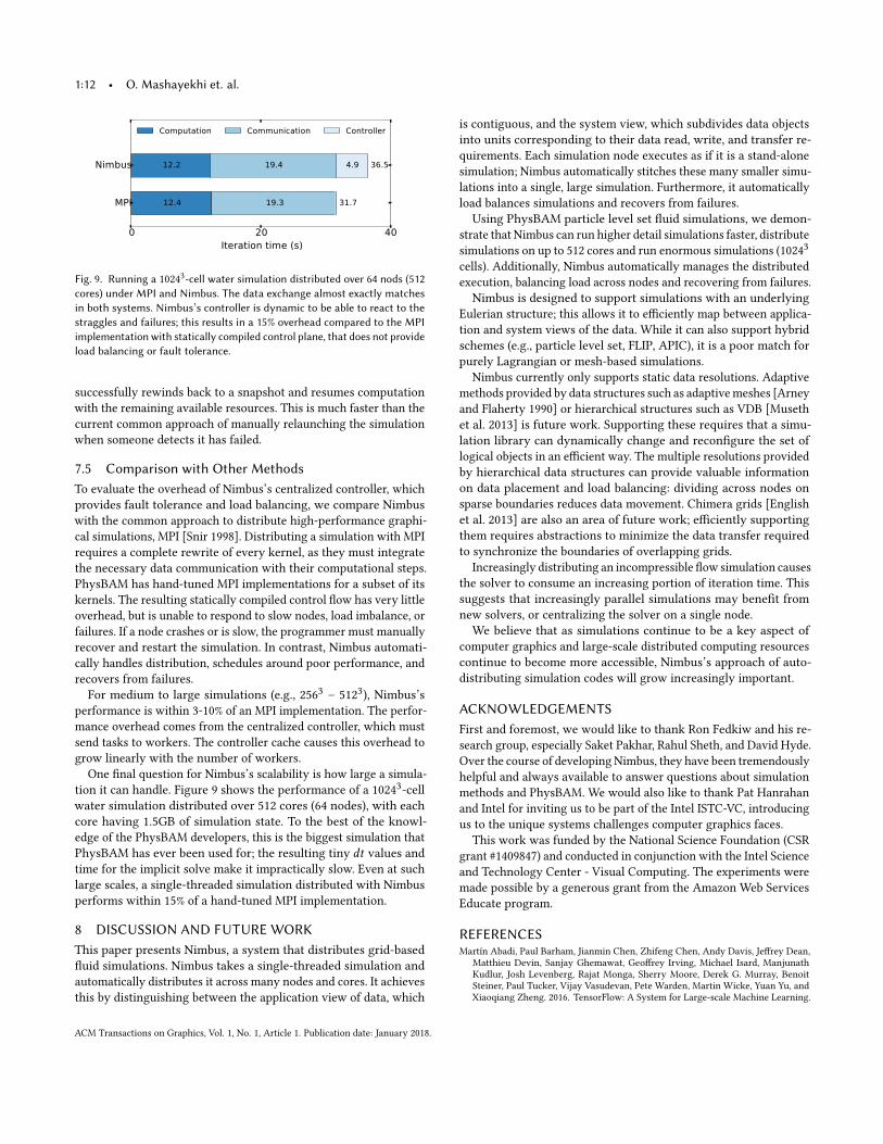
Fig. 9. Running a 10243-cell water simulation distributed over 64 nods (512cores) under MPI and Nimbus. The data exchange almost exactly matchesin both systems. Nimbus’s controller is dynamic to be able to react to thestraggles and failures; this results in a 15% overhead compared to the MPIimplementation with statically compiled control plane, that does not provideload balancing or fault tolerance.

successfully rewinds back to a snapshot and resumes computationwith the remaining available resources. This is much faster than thecurrent common approach of manually relaunching the simulationwhen someone detects it has failed.

7.5 Comparison with Other MethodsTo evaluate the overhead of Nimbus’s centralized controller, whichprovides fault tolerance and load balancing, we compare Nimbuswith the common approach to distribute high-performance graphi-cal simulations, MPI [Snir 1998]. Distributing a simulation with MPIrequires a complete rewrite of every kernel, as they must integratethe necessary data communication with their computational steps.PhysBAM has hand-tuned MPI implementations for a subset of itskernels. The resulting statically compiled control flow has very littleoverhead, but is unable to respond to slow nodes, load imbalance, orfailures. If a node crashes or is slow, the programmer must manuallyrecover and restart the simulation. In contrast, Nimbus automati-cally handles distribution, schedules around poor performance, andrecovers from failures.For medium to large simulations (e.g., 2563 – 5123), Nimbus’s

performance is within 3-10% of an MPI implementation. The perfor-mance overhead comes from the centralized controller, which mustsend tasks to workers. The controller cache causes this overhead togrow linearly with the number of workers.

One final question for Nimbus’s scalability is how large a simula-tion it can handle. Figure 9 shows the performance of a 10243-cellwater simulation distributed over 512 cores (64 nodes), with eachcore having 1.5GB of simulation state. To the best of the knowl-edge of the PhysBAM developers, this is the biggest simulation thatPhysBAM has ever been used for; the resulting tiny dt values andtime for the implicit solve make it impractically slow. Even at suchlarge scales, a single-threaded simulation distributed with Nimbusperforms within 15% of a hand-tuned MPI implementation.

8 DISCUSSION AND FUTURE WORKThis paper presents Nimbus, a system that distributes grid-basedfluid simulations. Nimbus takes a single-threaded simulation andautomatically distributes it across many nodes and cores. It achievesthis by distinguishing between the application view of data, which

is contiguous, and the system view, which subdivides data objectsinto units corresponding to their data read, write, and transfer re-quirements. Each simulation node executes as if it is a stand-alonesimulation; Nimbus automatically stitches these many smaller simu-lations into a single, large simulation. Furthermore, it automaticallyload balances simulations and recovers from failures.Using PhysBAM particle level set fluid simulations, we demon-

strate that Nimbus can run higher detail simulations faster, distributesimulations on up to 512 cores and run enormous simulations (10243cells). Additionally, Nimbus automatically manages the distributedexecution, balancing load across nodes and recovering from failures.Nimbus is designed to support simulations with an underlying

Eulerian structure; this allows it to efficiently map between applica-tion and system views of the data. While it can also support hybridschemes (e.g., particle level set, FLIP, APIC), it is a poor match forpurely Lagrangian or mesh-based simulations.

Nimbus currently only supports static data resolutions. Adaptivemethods provided by data structures such as adaptivemeshes [Arneyand Flaherty 1990] or hierarchical structures such as VDB [Musethet al. 2013] is future work. Supporting these requires that a simu-lation library can dynamically change and reconfigure the set oflogical objects in an efficient way. The multiple resolutions providedby hierarchical data structures can provide valuable informationon data placement and load balancing: dividing across nodes onsparse boundaries reduces data movement. Chimera grids [Englishet al. 2013] are also an area of future work; efficiently supportingthem requires abstractions to minimize the data transfer requiredto synchronize the boundaries of overlapping grids.

Increasingly distributing an incompressible flow simulation causesthe solver to consume an increasing portion of iteration time. Thissuggests that increasingly parallel simulations may benefit fromnew solvers, or centralizing the solver on a single node.We believe that as simulations continue to be a key aspect of

computer graphics and large-scale distributed computing resourcescontinue to become more accessible, Nimbus’s approach of auto-distributing simulation codes will grow increasingly important.

ACKNOWLEDGEMENTSFirst and foremost, we would like to thank Ron Fedkiw and his re-search group, especially Saket Pakhar, Rahul Sheth, and David Hyde.Over the course of developing Nimbus, they have been tremendouslyhelpful and always available to answer questions about simulationmethods and PhysBAM. We would also like to thank Pat Hanrahanand Intel for inviting us to be part of the Intel ISTC-VC, introducingus to the unique systems challenges computer graphics faces.

This work was funded by the National Science Foundation (CSRgrant #1409847) and conducted in conjunction with the Intel Scienceand Technology Center - Visual Computing. The experiments weremade possible by a generous grant from the Amazon Web ServicesEducate program.

REFERENCESMartín Abadi, Paul Barham, Jianmin Chen, Zhifeng Chen, Andy Davis, Jeffrey Dean,

Matthieu Devin, Sanjay Ghemawat, Geoffrey Irving, Michael Isard, ManjunathKudlur, Josh Levenberg, Rajat Monga, Sherry Moore, Derek G. Murray, BenoitSteiner, Paul Tucker, Vijay Vasudevan, Pete Warden, Martin Wicke, Yuan Yu, andXiaoqiang Zheng. 2016. TensorFlow: A System for Large-scale Machine Learning.



In Proceedings of the 12th USENIX Conference on Operating Systems Design andImplementation (OSDI’16). USENIX Association, 265–283. http://dl.acm.org/citation.cfm?id=3026877.3026899

Academy of Motion Picture Arts and Sciences. 2017. Oscar Sci-Tech Awards. (2017).http://www.oscars.org/sci-tech

Jérémie Allard and Bruno Raffin. 2005. A Shader-based Parallel Rendering Framework.In VIS 05. IEEE Visualization, 2005. IEEE, 127–134. https://doi.org/10.1109/VISUAL.2005.1532787

Ganesh Ananthanarayanan, Ali Ghodsi, Scott Shenker, and Ion Stoica. 2013. Effec-tive Straggler Mitigation: Attack of the Clones. In Proceedings of the 10th USENIXConference on Networked Systems Design and Implementation (NSDI’13). USENIXAssociation, 185–198. http://dl.acm.org/citation.cfm?id=2482626.2482645

Ganesh Ananthanarayanan, Srikanth Kandula, Albert Greenberg, Ion Stoica, Yi Lu,Bikas Saha, and Edward Harris. 2010. Reining in the Outliers in Map-reduce ClustersUsing Mantri. In Proceedings of the 9th USENIX Conference on Operating SystemsDesign and Implementation (OSDI’10). USENIX Association, 265–278. http://dl.acm.org/citation.cfm?id=1924943.1924962

Jason Ansel, Kapil Arya, and Gene Cooperman. 2009. DMTCP: Transparent Check-pointing for Cluster Computations and the Desktop. In Proceedings of the 2009IEEE International Symposium on Parallel&Distributed Processing (IPDPS’09). IEEEComputer Society, 1–12. https://doi.org/10.1109/IPDPS.2009.5161063

David C. Arney and Joseph E. Flaherty. 1990. An Adaptive Mesh-moving and LocalRefinement Method for Time-dependent Partial Differential Equations. ACM Trans.Math. Softw. 16, 1 (March 1990), 48–71. https://doi.org/10.1145/77626.77631

Michael Edward Bauer. 2014. Legion: Programming Distributed Heterogeneous Architec-tures with Logical Regions. Ph.D. Dissertation.

Gilbert Louis Bernstein, Chinmayee Shah, Crystal Lemire, Zachary Devito, MatthewFisher, Philip Levis, and Pat Hanrahan. 2016. Ebb: A DSL for Physical Simulation onCPUs and GPUs. ACM Transactions on Graphics (TOG) 35, 2, Article 21 (May 2016),12 pages. https://doi.org/10.1145/2892632

Umit V Catalyurek, Erik G Boman, Karen D Devine, Doruk Bozdag, Robert Heaphy, andLee Ann Riesen. 2007. Hypergraph-based Dynamic Load Balancing for AdaptiveScientific Computations. In Parallel and Distributed Processing Symposium, 2007.IPDPS 2007. IEEE International. 1–11. https://doi.org/10.1109/IPDPS.2007.370258

Philippe Charles, Christian Grothoff, Vijay Saraswat, Christopher Donawa, Allan Kiel-stra, Kemal Ebcioglu, Christoph Von Praun, and Vivek Sarkar. 2005. X10: AnObject-oriented Approach to Non-uniform Cluster Computing. In Acm SigplanNotices, Vol. 40. ACM, 519–538.

NVIDIA Corporation. 2017. CUDA Programming Guide. (2017). https://docs.nvidia.com/cuda/cuda-c-programming-guide/

JeffreyDean, Greg Corrado, RajatMonga, Kai Chen,Matthieu Devin,MarkMao, AndrewSenior, Paul Tucker, Ke Yang, Quoc V Le, et al. 2012. Large scale distributed deepnetworks. In Advances in neural information processing systems. 1223–1231.

Jeffrey Dean and Sanjay Ghemawat. 2008. MapReduce: Simplified Data Processing onLarge Clusters. Commun. ACM 51, 1 (2008), 107–113.

Steven J Deitz, Bradford L Chamberlain, and Lawrence Snyder. 2004. Abstractionsfor Dynamic Data Distribution. In High-Level Parallel Programming Models andSupportive Environments, 2004. Proceedings. Ninth International Workshop on. IEEE,42–51.

Tyler Denniston, Shoaib Kamil, and Saman Amarasinghe. 2016. Distributed Halide.In Proceedings of the 21st ACM SIGPLAN Symposium on Principles and Practice ofParallel Programming (PPoPP’16). ACM, Article 5, 12 pages. https://doi.org/10.1145/2851141.2851157

Mathieu Desbrun and Marie-Paule Gascuel. 1996. Smoothed Particles: A New Paradigmfor Animating Highly Deformable Bodies. In Computer Animation and Simulation’96.Springer, 61–76.

Zachary DeVito, Niels Joubert, Francisco Palacios, Stephen Oakley, Montserrat Medina,Mike Barrientos, Erich Elsen, Frank Ham, Alex Aiken, Karthik Duraisamy, et al. 2011.Liszt: A Domain Specific Language for Building Portable Mesh-based PDE Solvers.In Proceedings of 2011 International Conference for High Performance Computing,Networking, Storage and Analysis (SC’11). ACM, 9.

Sheng Di, Yves Robert, Frédéric Vivien, Derrick Kondo, Cho-Li Wang, and FranckCappello. 2013. Optimization of Cloud Task Processing with Checkpoint-RestartMechanism. In High Performance Computing, Networking, Storage and Analysis (SC),2013 International Conference for. IEEE, 1–12.

James Dinan, D. Brian Larkins, P. Sadayappan, Sriram Krishnamoorthy, and JarekNieplocha. 2009. Scalable Work Stealing. In Proceedings of the Conference on HighPerformance Computing Networking, Storage and Analysis (SC’09). ACM, Article 53,11 pages. https://doi.org/10.1145/1654059.1654113

Jens Dittrich and Jorge-Arnulfo Quiané-Ruiz. 2012. Efficient Big Data Processing inHadoop MapReduce. Proceedings of the VLDB Endowment 5, 12 (2012), 2014–2015.

Pradeep Dubey, Pat Hanrahan, Ronald Fedkiw, Michael Lentine, and Craig Schroeder.2011. PhysBAM: Physically Based Simulation. In ACM SIGGRAPH 2011 Courses.ACM, 10.

R Elliot English, Linhai Qiu, Yue Yu, and Ronald Fedkiw. 2013. Chimera Grids for WaterSimulation. In Proceedings of the 12th ACM SIGGRAPH/Eurographics Symposium on

Computer Animation. ACM, 85–94.Douglas Enright, Ronald Fedkiw, Joel Ferziger, and IanMitchell. 2002a. AHybrid Particle

Level SetMethod for Improved Interface Capturing. Journal of Computational physics183, 1 (2002), 83–116.

Douglas Enright, Stephen Marschner, and Ronald Fedkiw. 2002b. Animation andRendering of Complex Water Surfaces. In Proceedings of the 29th Annual Conferenceon Computer Graphics and Interactive Techniques (SIGGRAPH’02). ACM, 736–744.https://doi.org/10.1145/566570.566645

Kayvon Fatahalian, Daniel Reiter Horn, Timothy J Knight, Larkhoon Leem, MikeHouston, Ji Young Park, Mattan Erez, Manman Ren, Alex Aiken, William J Dally,et al. 2006. Sequoia: Programming the Memory Hierarchy. In Proceedings of the 2006ACM/IEEE Conference on Supercomputing. ACM, 83.

J Davison de St Germain, John McCorquodale, Steven G Parker, and Christopher RJohnson. 2000. Uintah: A Massively Parallel Problem Solving Environment. InHigh-Performance Distributed Computing, 2000. Proceedings. The Ninth InternationalSymposium on. IEEE, 33–41.

Sanjay Ghemawat and Jeff Dean. 2017. LevelDB. (2017). https://github.com/google/leveldb

Joseph E. Gonzalez, Yucheng Low, Haijie Gu, Danny Bickson, and Carlos Guestrin.2012. PowerGraph: Distributed Graph-parallel Computation on Natural Graphs.In Proceedings of the 10th USENIX Conference on Operating Systems Design andImplementation (OSDI’12). USENIX Association, 17–30. http://dl.acm.org/citation.cfm?id=2387880.2387883

Nolan Goodnight. 2007. CUDA/OpenGL Fluid Simulation. NVIDIA Corporation (2007).Pat Hanrahan and Jim Lawson. 1990. A Language for Shading and Lighting Calculations.

In ACM SIGGRAPH Computer Graphics, Vol. 24. ACM, 289–298.Paul H Hargrove and Jason C Duell. 2006. Berkeley Lab Checkpoint/Restart (BLCR) for

Linux Clusters. In Journal of Physics: Conference Series, Vol. 46. IOP Publishing, 494.Francis H Harlow. 1962. The Particle-in-cell Method for Numerical Solution of Problems

in Fluid Dynamics. Technical Report. Los Alamos Scientific Lab., N. Mex.Christopher J Hughes, Radek Grzeszczuk, Eftychios Sifakis, Daehyun Kim, Sanjeev

Kumar, Andrew P Selle, Jatin Chhugani, Matthew Holliman, and Yen-Kuang Chen.2007. Physical Simulation for Animation and Visual Effects: Parallelization andCharacterization for Chip Multiprocessors. In ACM SIGARCH Computer ArchitectureNews, Vol. 35. ACM, 220–231.

Greg Humphreys, Mike Houston, Ren Ng, Randall Frank, Sean Ahern, Peter D Kirchner,and James T Klosowski. 2002. Chromium: A Stream-Processing Framework forInteractive Rendering on Clusters. ACM Transactions on Graphics (TOG) 21, 3 (2002),693–702.

Emmanuel Jeannot, EstebanMeneses, GuillaumeMercier, François Tessier, and GengbinZheng. 2013. Communication and Topology-aware Load Balancing in Charm++withTreeMatch. In Cluster Computing (CLUSTER), 2013 IEEE International Conference on.1–8. https://doi.org/10.1109/CLUSTER.2013.6702666

Chenfanfu Jiang, Craig Schroeder, Andrew Selle, Joseph Teran, and Alexey Stomakhin.2015. The Affine Particle-in-cell Method. ACM Transactions on Graphics (TOG) 34, 4(2015), 51.

Laxmikant V Kale and Sanjeev Krishnan. 1993. CHARM++: A Portable Concurrent ObjectOriented System Based on C++. Vol. 28. ACM.

Shoaib Kamil. 2017. StencilProbe: A Microbenchmark for Stencil Applications. (2017).http://people.csail.mit.edu/skamil/projects/stencilprobe/

George Karypis and Vipin Kumar. 1996. Parallel Multilevel K-way Partitioning Schemefor Irregular Graphs. In Proceedings of the 1996 ACM/IEEE Conference on Supercom-puting (SC’96). IEEE Computer Society, Article 35. https://doi.org/10.1145/369028.369103

Fredrik Kjolstad, Shoaib Kamil, Jonathan Ragan-Kelley, David IW Levin, Shinjiro Sueda,Desai Chen, Etienne Vouga, Danny M Kaufman, Gurtej Kanwar, Wojciech Matusik,et al. 2016. Simit: A Language for Physical Simulation. ACM Transactions on Graphics(TOG) 35, 2 (2016), 20.

Honglak Lee, Roger Grosse, Rajesh Ranganath, and Andrew Y. Ng. 2009. ConvolutionalDeep Belief Networks for Scalable Unsupervised Learning of Hierarchical Repre-sentations. In Proceedings of the 26th Annual International Conference on MachineLearning (ICML’09). ACM, 609–616. https://doi.org/10.1145/1553374.1553453

Jonathan Lifflander, Sriram Krishnamoorthy, and Laxmikant V. Kale. 2012. WorkStealing and Persistence-based Load Balancers for Iterative Overdecomposed Ap-plications. In Proceedings of the 21st International Symposium on High-PerformanceParallel and Distributed Computing (HPDC’12). ACM, 137–148. https://doi.org/10.1145/2287076.2287103

Frank Losasso, Frédéric Gibou, and Ron Fedkiw. 2004. Simulating Water and Smokewith an Octree Data Structure. In ACM Transactions on Graphics (TOG), Vol. 23.ACM, 457–462.

David Luebke. 2008. CUDA: Scalable Parallel Programming for High-performanceScientific Computing. In 2008 5th IEEE International Symposium on BiomedicalImaging: From Nano to Macro. IEEE, 836–838.

Grzegorz Malewicz, Matthew H Austern, Aart JC Bik, James C Dehnert, Ilan Horn, NatyLeiser, and Grzegorz Czajkowski. 2010. Pregel: A System for Large-scale GraphProcessing. In Proceedings of the 2010 ACM SIGMOD International Conference on



Management of data. ACM, 135–146.Omid Mashayekhi, Hang Qu, Chnimayee Shah, and Philip Levis. 2017. Execution Tem-

plates: Caching Control Plane Decisions for Strong Scaling of Data Analytics. In 2017USENIX Annual Technical Conference (ATC’17). USENIX Association, 513–526. https://www.usenix.org/conference/atc17/technical-sessions/presentation/mashayekhi

Derek G Murray, Frank McSherry, Rebecca Isaacs, Michael Isard, Paul Barham, andMartín Abadi. 2013. Naiad: A Timely Dataflow System. In Proceedings of the Twenty-Fourth ACM Symposium on Operating Systems Principles (SOSP’13). ACM, 439–455.

Ken Museth, Jeff Lait, John Johanson, Jeff Budsberg, Ron Henderson, Mihai Alden,Peter Cucka, David Hill, and Andrew Pearce. 2013. OpenVDB: An Open-sourceData Structure and Toolkit for High-resolution Volumes. In ACM SIGGRAPH 2013Courses. ACM, 19.

Lionel M. Ni and Kai Hwang. 1985. Optimal Load Balancing in a Multiple ProcessorSystem with Many Job Classes. IEEE Trans. Softw. Eng. 11, 5 (May 1985), 491–496.https://doi.org/10.1109/TSE.1985.232489

Kay Ousterhout, Ryan Rasti, Sylvia Ratnasamy, Scott Shenker, Byung-Gon Chun, andVMware ICSI. 2015. Making Sense of Performance in Data Analytics Frameworks.In Proceedings of the 12th USENIX Symposium on Networked Systems Design andImplementation (NSDI’15). 293–307.

Kay Ousterhout, Patrick Wendell, Matei Zaharia, and Ion Stoica. 2013. Sparrow: Dis-tributed, Low Latency Scheduling. In Proceedings of the Twenty-Fourth ACM Sympo-sium on Operating Systems Principles (SOSP’13). ACM, 69–84.

Saket Patkar, Mridul Aanjaneya, Dmitriy Karpman, and Ronald Fedkiw. 2013. A HybridLagrangian-Eulerian Formulation for Bubble Generation and Dynamics. In Proceed-ings of the 12th ACM SIGGRAPH/Eurographics Symposium on Computer Animation.ACM, 105–114.

Joshua Peraza, Ananta Tiwari, Michael Laurenzano, Laura Carrington, William AWard,and Roy Campbell. 2013. Understanding the Performance of Stencil Computations onIntel’s Xeon Phi. In Cluster Computing (CLUSTER), 2013 IEEE International Conferenceon. IEEE, 1–5.

Jonathan Ragan-Kelley, Connelly Barnes, Andrew Adams, Sylvain Paris, Frédo Durand,and Saman Amarasinghe. 2013. Halide: A Language and Compiler for OptimizingParallelism, Locality, and Recomputation in Image Processing Pipelines. ACMSIGPLAN Notices 48, 6 (2013), 519–530.

Jon Reisch, Stephen Marshall, Magnus Wrenninge, Tolga Göktekin, Michael Hall,Michael O’Brien, Jason Johnston, Jordan Rempel, and Andy Lin. 2016. Simulat-ing Rivers in the Good Dinosaur. In ACM SIGGRAPH 2016 Talks. ACM, 40.

Gabriel Rivera and Chau-Wen Tseng. 2000. Tiling Optimizations for 3D ScientificComputations. In Supercomputing, ACM/IEEE 2000 Conference. IEEE, 32–32.

Elliott Slaughter, Wonchan Lee, Sean Treichler, Michael Bauer, and Alex Aiken. 2015.Regent: A High-productivity Programming Language for HPC with Logical Regions.In Proceedings of the International Conference for High Performance Computing,Networking, Storage and Analysis (SC’15). ACM, 81.

Marc Snir. 1998. MPI–The Complete Reference: The MPI Core. Vol. 1. MIT press.Jos Stam. 1999. Stable Fluids. In Proceedings of the 26th Annual Conference on Computer

Graphics and Interactive Techniques. ACM Press/Addison-Wesley Publishing Co.,121–128.

Matt Stanton, Ben Humberston, Brandon Kase, James F O’Brien, Kayvon Fatahalian, andAdrien Treuille. 2014. Self-refining Games Using Player Analytics. ACM Transactionson Graphics (TOG) 33, 4 (2014), 73.

Yuan Tang, Rezaul Alam Chowdhury, Bradley C Kuszmaul, Chi-Keung Luk, andCharles E Leiserson. 2011. The Pochoir Stencil Compiler. In Proceedings of theTwenty-third Annual ACM Symposium on Parallelism in Algorithms and Architectures.ACM, 117–128.

The Khronos Group. 2017a. OpenCL. (2017). https://www.khronos.org/opencl/The Khronos Group. 2017b. OpenGL. (2017). https://www.opengl.org/Kashi Venkatesh Vishwanath and Nachiappan Nagappan. 2010. Characterizing Cloud

Computing Hardware Reliability. In Proceedings of the 1st ACM Symposium on CloudComputing (SoCC’10). ACM, 193–204. https://doi.org/10.1145/1807128.1807161

William WWhite. 2012. River Running Through It. (2012). https://www.cs.siue.edu/~wwhite/SIGGRAPH/SIGGRAPH2012Itinerary.pdf

Samuel Williams, John Shalf, Leonid Oliker, Shoaib Kamil, Parry Husbands, and Kather-ine Yelick. 2006. The Potential of the Cell Processor for Scientific Computing. InProceedings of the 3rd Conference on Computing Frontiers. ACM, 9–20.

JohnW Young. 1974. A First Order Approximation to the Optimum Checkpoint Interval.Commun. ACM 17, 9 (1974), 530–531.

Matei Zaharia, Mosharaf Chowdhury, Tathagata Das, Ankur Dave, Justin Ma, Mur-phy McCauley, Michael J Franklin, Scott Shenker, and Ion Stoica. 2012. ResilientDistributed Datasets: A Fault-tolerant Abstraction for In-memory Cluster Comput-ing. In Proceedings of the 9th USENIX Conference on Networked Systems Design andImplementation (NSDI’16). USENIX Association, 2–2.

Gengbin Zheng, Abhinav Bhatelé, Esteban Meneses, and Laxmikant V. Kalé. 2011.Periodic Hierarchical Load Balancing for Large Supercomputers. Int. J. High Perform.Comput. Appl. 25, 4 (Nov. 2011), 371–385. https://doi.org/10.1177/1094342010394383

Yongning Zhu and Robert Bridson. 2005. Animating Sand as a Fluid. InACMTransactionson Graphics (TOG), Vol. 24. ACM, 965–972.


automatically distributing eulerian and hybrid fluid ... · fluid simulation is a cornerstone of...

Documents