automatic vehicle detection using various object …1.4 image processing with mathcad and matlab....

International Journal on Future Revolution in Computer Science & Communication Engineering

Volume: 1 Issue: 1 16 – 28

_____________________________________________________________________________________

16 IJFRCSCE | June 2015, Available @ http://www.ijfrcsce.org _______________________________________________________________________________________

Automatic Vehicle Detection Using Various Object Detecting Algorithm and

Thresholding Methods

Aarti Sharma,

M. Tech Scholar (CSE), ECB

Rajasthan (India)

Abstract:-The digital image processing deals with developing a digital system to performs experiments and operations on a digital image with

the use of computer algorithms. An image is nothing more than a 2D mathematical function f(x,y) where x and y are two horizontally and

vertically co-ordinates. Object recognition is one of the most important applications of image processing.

Vehicle detection from a satellite image or aerial image is one of the most interesting and challenging research topics from past few years.

Vehicle detection from satellite image is one of the applications of object detection. The traffic and crowd is increasing everyday in all over the

world. Satellites images are normally used for weather forecasting and geographical applications. So, Satellites images may be also good for the

detecting traffic using Image processing. This thesis used simple morphological recognition method for vehicle detection using image processing

technique in Matlab which is best method for detection of cars, trucks and buses. We can easily compute the total numbers of vehicles in the

desired area in the satellite image and vehicles are shown under the bounding box as a tiny spots. Here we compare two algorithms like pixel

thresholding and Otsu thresholding method. According to our result Pixel level thresholding is better than Otsu method.

Keywords:- Vehicles at surface, object detection algorithm, thresholding values, airel images.

__________________________________________________*****_________________________________________________

1. Introduction

1.1 Introduction of Image processing

In world of computer science Image processing is a quickly

growing area. Its growth has filled by technological advances in,

computer processors, digital imaging and mass storage devices.

Analog imaging is over taking by digital systems, for their

affordability & flexibility. Most seen examples in daily routine, are

medicines, video production remote sensing, photography, film and

security monitoring. Huge volumes of digital images data every

day produced by these and other sources, it’s too huge that, we

cannot check it manually [1].

1.2 Digital images

An image may be defined as a two-dimensional function, f(x, y),

where x and y are spatial (plane) coordinates, and the amplitude of

at any pair of coordinates (x, y) is called the intensity or gray level

of the image at that point. When x, y, and the amplitude values of f

are all finite, discrete quantities, we call the image a digital image.

The field of digital image processing refers to processing digital

images by means of a digital computer. Note that a digital image is

composed of a finite number of elements, each of which has a

particular location and value. These elements are referred to as

picture elements, image elements, pels, and pixels. Pixel is the term

most widely used to denote the elements of a digital image [2].

Three types of passive image sensing technologies are given

below, which have been made for target detection.

(1)Image Processing: Video Camera

Nowadays using video cameras to collect data for recognition

studies can be achieved at a lower cost compared to other image

sensing techniques [Nooralahiyan et al., 1997]. On the other hand,

the use of video camera images is not suitable under certain

monitoring conditions, for example during the night or foggy

conditions [Koch et al., 2006; Cheng et al., 2005]; which may

imply the unsuitability of them for the current research.

(2)Image Processing: Satellite

Satellite image detection is suitable when surveillance of a wide

area is required although the installation & maintenance costs may

be high [Roper, 2005]. The other disadvantages are the inability to

monitor & the low ground resolution on a cloudy day.

1.2.1Advantages with digital imaging

Benefits of digital image processing: low cost processing,

consistently high quality of the image, & the ability to manipulate

all aspects of the process. As long as computer processing speed

was increasing, cost of storage memory started dropping, this field

started growing [6].

There are various benefits with digital cameras compared to other

means of acquiring data. Main purposes were to make large spatial

resolution of CCD cameras. A resolution of 3120 X 2068 pixels

allows for a rather large span in the size of the features detected by

the cameras. This is very crucial for reliable fractal analysis of

scaling relations. The pixels size 9X 9m is of the same order as the

grain size in photographic films. The main advantages of the CCD

cameras are making it superior quality to video cam-recorders or

ordinary cameras.

1.3 Image Processing Techniques

This portion handles acquisition, processing & formation of

images. It is shown the best way in diagram where the processes

involved & evolution of the considered information (images).



_____________________________________________________________________________________


Figure 1: Image processing technique [7]

1.4 Image processing with MathCAD and MatLab.

The MathCAD & MatLab environments are perfectly suited to

image processing. Particularly, MatLab's matrix-oriented language

is perfectly suited for manipulating images, which are not more

than visual renderings of matrices. The result is a very easy &

economical way of expressing image processing operations. In

addition both programs have Image Processing Toolboxes which

provide a flexible & powerful environment for image analysis &

processing. Both programs were used to perform different

calculations on images [8].

There are various benefits of using MatLab & MathCAD for image

analysis. One is the ability to have directed access to any portion of

available information what in general is not possible with many

commercial image analysis systems. We can stop any calculation

anytime with the help of this program, change a portion of the

calculation procedure and then restart the calculations from the

point which was affected by the changes without recompiling the

code as it usually happens with programming in C, or even

restarting the calculations from the starting. New techniques are

developed and also these types of abilities are very helpful in

researches. Main disadvantage of this programs is the relatively

slow computational speed compared to compiled C code. It is

because of the need of the code to be translated first into a machine

code and only then to be executed. Therefore, complex image

processing applications can be better implemented by the use of

high level programming languages as C or C++, rather than using

the softwares like MathCAD or MatLab.

2. Literature survey

This survey included various types of images, image segmentation,

threshold techniques and previous work for detecting the vehicles.

A literature survey has been conducted in order to understand the

current and past research trends in the area of automated moving

vehicle recognition systems. And this chapter discuss about the

previous work for detecting the vehicles using pixel level and Otsu

thresholding techniques.

2.1 Previous work

Semantic analysis of changes in satellite imagery requires the

detection of changes as a first step. Change detection is a well

studied problem in computer vision and many modern change

detection algorithms exist. The most notable of these rely on a

technique called background modeling. In this approach, a number

of images of the scene are used to learn what the normal

background appearance of the scene should look like so that given

a new image, the pixels with abnormal appearance can be detected

as changes [22].

Most of the literature addresses 2-d background modeling problem

in which the images of the scene can be registered to a common 2-

d frame. This is trivially the case with stationary cameras or is

possible through various registration techniques. Early attempts at

2-d background modeling [25, 26, and 27] use a single Gaussian

density at each pixel to model background intensity plus

acquisition noise. These densities are updated with simple adaptive

filters as new observations of the pixel are made. In this approach,

the single Gaussian cannot model the pixel variation present in

many real world scenes such as frequently occluded surfaces

(roads), slow moving objects, and vegetation blowing in the wind.

Stauffer and Grimson [28] proposed the first fully general

algorithm to model a more realistic dynamic background. They

used a mixture of Gaussians [29] density at each pixel which is a

widely used and well studied distribution for modeling multi-

modal data. Because of its fast and robust performance on all types

of realistic scenes, the Stauffer-Grimson algorithm has become the

standard technique for change detection.

In the case of non-stationary cameras, the registration step required

for 2-d background modeling works reasonably well only if the

camera motion is mostly limited to pan/tilt or the scene is mostly

planar. This is because the image registration techniques rely on

global image transformations such as homographies, or polynomial

warping for satellite imagery. The latter allows for more distortion

of the image but is still a global transformation and cannot do local

alignments of objects with 3-d relief between images, which is the

case for satellite imagery. These limitations call for a 3-d solution

to the problem.

3-d change detection is a relatively less researched field in

computer vision. Earlier approaches [30,31] used manually

constructed 3-d site models to make correspondences between

images so that change detection algorithm can be applied. The

overhead of constructing 3-d geometry is infeasible for this kind of

approach to be used in modern applications. Heller et al. [32] use

stereo pairs of satellite images to reconstruct 3-d geometry of the

scene and then compare reconstructed geometry from different

pairs of images to detect 3-d changes to the scene. This algorithm

is more applicable but it depends on having stereo pairs and it

cannot detect appearance changes on the surfaces of the scene such

as moving vehicles and shadows. Recently, a new approach that

combines the power of Stauffer-Grimson style appearance

modeling with automated 3-d geometry discovery has been

proposed [32]. This volumetric appearance modeling (VAM)

approach is suitable for change detection from satellite imagery for

several reasons. First, it is not assumed that there is a fixed set of



_____________________________________________________________________________________


images available at the beginning and the model of the world is

built up incrementally as images are observed in an unbounded

sequence. This type of processing is called an on-line algorithm in

computer science terminology. This makes it possible to discard

each image after processing and reduces storage requirements

significantly making the method applicable to satellite domain

where image sizes are on the order of GBytes. Second, VAM

makes no assumptions about frame-to-frame continuity. Third,

even though a camera model, namely a cubic rational polynomial

camera [33] for the case of satellite imagery, is supplied with each

image to be processed, in general it is necessary to calibrate and

register such projection models due to errors in platform motion

and internal parameters. These adjustments are outside the scope of

this paper and in this work it is assumed that the cameras are

correct.

However, the VAM framework is capable of supporting automated

camera calibration and registration [34]. Finally, it has been shown

[35] that the framework tolerates the amount of variability in

viewpoint, lighting, and atmospheric conditions such as haze that is

typically observed in satellite imagery.

2.2 Related Work for Object Recognition

Semantic analysis of changes in satellite imagery requires the

classification of change regions as the second step. The objects of

interest in this analysis are vehicles. But the classification

technique used is general and applies to several object categories

such as buildings, roads, bridges, etc. which could also be objects

of interest in satellite imagery [24]. From a probabilistic point of

view, being on a changing surface in the scene, and being on an

object surface are independent events for a pixel in an image.

Hence the output map of a change classification algorithm can

simply be computed as the product of the change map as given by

the Voxel World and the classification map as given by a

conventional classification algorithm. However the classification

module can proceed in a completely independent manner as well

and the algorithm used is in the realm of the classical classification

algorithms.

Object recognition is the problem of declaring existence of an

instance from an object class in a given image patch. The input

image may be larger and contain many instances of the class as in

the case of satellite imagery. However the algorithms usually

convolve the input image with the classification module which

boils down to the classification of a patch in the image that is of the

extent of the object instance. Thus, the classification module

explicitly achieves position invariance during recognition. By

carrying out processing at multiple scales, it is also possible to

achieve scale invariance. In the following discussion, the object

image will refer to the image patch that contains the whole extent

of the object as seen in the image and the image domain will refer

to this patch and not the whole input image.

2.3 Related work on Road Vehicle Recognition

This section describes research on road vehicles rather than

military ones. In general, research on road vehicle recognition is

performed for traffic management or automated driver assistance

system.

(a) [Sampan, 1997] A PhD thesis was published for traffic

monitoring by using a circular array, consisting of 152

microphones, but 143 of them were of interest. After the data were

pre-processed to only maintain the components between 2700Hz

and 5400Hz, the 30-dimension feature vectors were extracted from

the energy over each 0.2 seconds in the time domain. PCA was

processed to reduce the dimension to 24 before performing

classification with either kNN, Multilayer Perceptron (MLP) or

Adaptive Fuzzy Logic System (AFLS). Although the exact number

of vehicles in each class was not clear, it was stated that they

varied between each class; and there were data of 1327 vehicles in

total. Problems caused by this inequality of the sizes of training

sets was addressed in the thesis by considering the effect on the

training as well as introducing the learning factor, a method

intended to take care of the issue. Moreover, it attempted to deal

with the inequality derived from the fact some classes are easier to

be learned than others by allocating misclassification costs for each

pattern although there was no logical explanation regarding how

they were determined. The obtained classification accuracies were

97.95%, 92.24% and 78.67% for 2-class, 4- class, and 5-class

experiments respectively. Althugh the use of such a large number

of microphones may not be appropriate for developing a cost

effective and compact recognition system, this study played a good

role in initiating research on acoustic road vehicle recognition with

fairly accurate results.

(b) [Nooralahiyan et al., 1997, 1998] Researchers at the

University of Leeds published two similar papers on their acoustic

road vehicle classification studies for traffic monitoring in the late

1990s. The focus was on classification only thus detection

algorithms were not included. The study was motivated by the

progress in automated speech recognition research that apparently

let them believe feasibility of the short term spectrum, particularly

at low frequencies, for the task. Therefore, the resultant algorithm

choice was made heuristically but with influence of speech

recognition studies. In the first paper [Nooralahiyan et al., 1997],

they first conducted a feasibility study using acoustic signals of

four vehicles; such as a small saloon, a medium saloon, a

motorcycles, and a light goods vehicle. All of the recordings were

collected under relatively controlled conditions, particularly in

terms of the level of background noise and vehicle speed. At this

stage, the feature extraction methods used were: FFT and

autocorrelation method Linear Predictive Coding (LPC) both in

MATLAB, and also software for computational modelling of

hearing, which was developed by Patterson et al. [Patterson et al.,

1995]. For the latter, Equivalent Rectangular Bandwidth (ERB)

based gammatone filterbanks, covering between 100Hz and

12kHz, were used to simulate the movement of the basilar

membrane in the cochlea. Moreover, the same software platform

was also used to simulate auditory nerve activity patterns of the

cochlea’s inner hair cells. Within these methods, FFT was omitted

after the initial stage because its classification outcome was not

satisfactory. An unsupervised Kohonen Self-Organising Map

(SOM) was used for this first phase of the study.

They then carried out another set of experiments using signals

collected at various urban road sites where they had little control

compared with the first stage [Nooralahiyan et al., 1998]. In total,

over 200 recordings of various vehicles travelling at different



_____________________________________________________________________________________


speed of no faster than 40 miles per hour (i.e. approximately 64 km

per hour), collected at more than 20 sites were utilised. The

collected feature vectors were classified by the supervised Time

Delay Neural Network (TDNN) with two hidden layers and no

feedback, between the following four classes; buses or lorries,

saloon cars, motorcycles, and light goods vehicle or vans. The

reported classification accuracies achieved, particularly with

adaptively changed threshold, were above 84%. These results were

seen as good, therefore, it might be a good reference for the the

current research.

(c) [Wu et al., 1998, 1999] Another example was reported in two

similar papers published firstly in a conference proceedings and

then in a journal. The adapted method was called “eigenfaces

methods”, which had been used in human face image recognition

beforehand. It is also known as Karhunen-Loeve expansion or

PCA. The feature vectors of acoustic signals were collected with

FFT power spectrum, which was then normalised per frame to unit

power. Some adjustment was also applied to reduce the impact of

insignificant parts before PCA was performed. The class of

unknown samples was determined according to the distance of the

new feature vector from the reference, which was prepared in

advance during training by using only selected data, recorded at the

same location under very similar conditions. Recordings of saloon

type cars were used as the training samples during the experiment.

The distributions of training and test sample sets were exhibited in

graphs, but no numerical values for classification accuracy nor

sample size was included. It was pointed out that the algorithm was

susceptible to the change in recording conditions; furthermore,

more data would be required to study sample distributions that

usefully display the signals’ distinguishable attributes. (d) [Jacyna

et al., 2005; Necioglu et al., 2005] A group of researchers at the

MITRE Corporation in the USA have published work on

developing acoustic road vehicle classification algorithms for

networked sensor systems [Jacyna et al., 2005]. Their approach

was based on a hierarchical network topology, and the

classification was performed between two road vehicle classes: the

“light” and the “heavy”. Firstly they looked into algorithm

development for a simple classification that can be performed at

each sensor node. The feature vectors were extracted by a

combination of FFT and 8-band filterbank, and then classified by a

so-called “linear-weighted classifier”. Although there was not

much information about the actual experimental results nor the

total number of different vehicles involved in the experiment, other

than mentioning the number of 125ms long audio file segments for

car and truck signals; it was reported that they managed to achieve

the minimum error rate of approximately 13%.

Secondly, according to another paper [Necioglu et al., 2005], a

more sophisticated classification algorithm that can be processed

on the features collected by the each node described above, but at

the next stage of the hierarchical network topology, was examined.

Although the feature extraction algorithm was similar to that of the

first one, this time they disclosed more information regarding the

experiment and the data set, in which the effects of small parameter

variation were also examined. The selected classification algorithm

for this stage was ML estimation with GMM. It was reported that

when the feature vectors, which were the filterbank output of

spectral energy, were scaled logarithmically; the minimum error

rate was found to be nearly 7%.

(e) [Sobreira-Seoane et al., 2008] An algorithm that has some

degree of similarity to the one studied for the current research in a

sense as they both consist of two stages, such as vehicle presence

detection and classification, was reported at a conference, which

some of the findings of this PhD research was also presented at. It

was realised that the obvious difference between the two

algorithms would be that Sobreira-Seoane purely relied on acoustic

signals. For vehicle detection, Short Time Energy (STE) and

envelope peaks were used. The chosen feature extraction

algorithms for classification stage were; Zero-Crossing Rate

(ZCR), “Spectral Centroid (centre gravity of spectral power

distribution)”, “Spectral Rolloff Point”, Subband Energy Ratio

(SBER), and MFCC. kNN and LDA algorithms were utilised as the

classifiers. The primary results showed that the combination of

kNN and three feature extraction algorithms; Spectral Rolloff

Point, SBER and MFCC, performed comparatively better, and

achieved nearly 90% accuracy.

(f) [Lu et al., 2008a,b] A vehicle detection algorithm, based on

studies in mammalian perception and neurology, was suggested in

articles in IEEE conference proceedings. This was another research

initiated from an augment that “there exists similarity between

vehicle and speech recognition”[Lu et al., 2008a, p.1336].

However, once again, they included no evidence nor discussion to

support such a view point. Their recommendation was to use

gammatone filterbank on STFT for feature extraction, dimension

reduction and the two-step decision making processes to first

detect the presence of vehicles before classifying them into four

vehicle groups. They conducted experiments to compare MFCC

and gammatone auditory filterbank on STFT. They showed that the

gammatone filterbanks outperformed MFCC under noisy

environment whereas MFCC was better in less noisy conditions. In

addition, a technique called Spectro-Temporal Representation

(STR) was described. This enhanced the correlation between

neighbouring signal frames, and the use of Nonlinear Hebbian

Learning (NHL) for reducing the dimension improved the

detection accuracy. In the best case, under less noisy environment

where the SNR was 10dB, it achieved about 95% accuracy, on

average under two kinds of noise although the performance

declined significantly as SNR decreased. They argued that the

algorithm could be expanded to classification tasks without

difficulty

(g) [Anami and Pagi, 2009] Recognition algorithms for two-wheel

vehicles were investigated. Vectors extracted by three time domain

methods, such as ZCR, STE and Root Mean Square(RMS) plus

two frequency domain feature extraction methods, “Mean and

Standard Deviation of Spectrum Centroid (CMEAN and CSD)”

were applied to the NN for classifying between two classes:

“bikes” and “scooters”. The recorded acoustic signals of 118

vehicles were utilised, of which 58 were for training and the rest

was for testing. It achieved 73.33% accuracy between the two

classes. The observed effects of vehcie ages and how well they

were maintained within the same class were also mentioned. Such

information can be useful for certain applications that have only



_____________________________________________________________________________________


known and limited targets, however, it does not apply to the

current project.

(f) [Amit Satpathy 2014] proposes two sets of novel edge-texture

features, Discriminative Robust Local Binary Pattern (DRLBP)

and Ternary Pattern (DRLTP), for object recognition. By

investigating the limitations of Local Binary Pattern (LBP), Local

Ternary Pattern (LTP) and Robust LBP (RLBP), DRLBP and

DRLTP are proposed as new features. They solve the problem of

discrimination between a bright object against a dark background

and vice-versa inherent in LBP and LTP. DRLBP also resolves the

problem of RLBP whereby LBP codes and their complements in

the same block are mapped to the same code. Furthermore, the

proposed features retain contrast information necessary for proper

representation of object contours that LBP, LTP, and RLBP

discard. Our proposed features are tested on seven challenging data

sets: INRIA Human, Caltech Pedestrian, UIUC Car, Caltech 101,

Caltech 256, Brodatz, and KTH-TIPS2- a. Results demonstrate that

the proposed features outperform the compared approaches on

most data sets.

(g) [Xueyun Chen, Shiming Xiang, Cheng-Lin Liu, and Chun-

Hong Pan 2014] Detecting small objects such as vehicles in

satellite images is a difficult problem. Many features (such as

histogram of oriented gradient, local binary pattern, scale-invariant

feature transform, etc.) have been used to improve the performance

of object detection, but mostly in simple environments such as

those on roads. Kembhavi et al. proposed that no satisfactory

accuracy has been achieved in complex environments such as the

City of San Francisco. Deep convolutional neural networks

(DNNs) can learn rich features from the training data automatically

and has achieved state-of-the-art performance in many image

classification databases. Though the DNN has shown robustness to

distortion, it only extracts features of the same scale, and hence is

insufficient to tolerate large-scale variance of object. In this letter,

we present a hybrid DNN (HDNN), by dividing the maps of the

last convolutional layer and the maxpooling layer of DNN into

multiple blocks of variable receptive field sizes or max-pooling

field sizes, to enable the HDNN to extract variable-scale features.

Comparative experimental results indicate that our proposed

HDNN significantly outperforms the traditional DNN on vehicle

detection.

3. Experimental Result and Analysis

Satellite resolution and object-oriented detection method are being

better day by day in satellite images. Comparing to traditional data

acquired methods, in large area satellite images the heavy traffic

data can be faster and widely acquired. In this work first of all the

image quality is improved, and then the multiscale segmentation

technology is used and the vehicles are detected from satellite

images from supervised classification method [44]. The simple

morphological recognition method is used for vehicle detection

using image processing technique in Matlab which is one of the

best methods for detection of trucks, cars, bikes and buses etc.

4.1 Data Information

This thesis work is used five images named New 5, D10, New

3, New 4 and New 7 as a reference. And step by step process

is described on the image New 5. Images are shown in 4.1,

4.2, 4.3, 4.4, 4.5 figures.

Figure 4.1: New 5 image (reference image no. 1)

Figure 4.2: D10 image (reference image no. 2)





_____________________________________________________________________________________



4.2 Methodology

Morphological recognition algorithms are used to develop an

automated system in MATLAB R2013a. In which satellite images

are taken as input and converted into gray scale image for pre-

processing. After conversion these images are converted into

binary images after image complement. After conversion canny

edge detection method has done and passed this detection to the

dilation process. The area is selected after filtration and dilation

where number of vehicles is maximum and vehicles are recognized

from the image in the form of bounding box. The number of

vehicles is counted by blob analysis. Here we are using reference

image New 5.

Figure 4.6: Block Diagram of vehicle detection from satellite image using canny edge

The steps in block diagram are elaborated below:

1) Satellite Image Acquisition:

a) Read Satellite image

b) Resize Image

2) Necessary Operations

a. RGB to Gray Scale conversion

3) Image segmentation process

a. Gray image to Binary conversion

b. Edge Detection

4) Image Enhancement

a. Filling Holes on images

b. Creating Holes Edge Detected Images

c. Filteration of image using Bewareopen

command using High pass filter

4.3 Process to detect vehicles from satellite images

Process to detect vehicle include many steps. Descriptions of these

steps are as following:

Figure 4.7: Acquired Image



_____________________________________________________________________________________


Figure 4.8: RGB to Gray Scale Conversion

Figure 4.8: Binary Converted Image

Figure 4.9: Canny Edge Detection

Figure 4.10: Filling contour holes for vehicle detection.

Figure 4.11: Filtration using high pass filter

Figure 4.12: cropped area

4.3.9 Detected Vehicles using Blob Analysis

Blob Analysis is a fundamental technique of machine

vision based on analysis of consistent image regions. As

such it is a tool of choice for applications in which the

objects being inspected are clearly discernible from the

background. Diverse set of Blob Analysis methods allows

creating tailored solutions for a wide range of visual

inspection problems.



_____________________________________________________________________________________


Figure 4.13: Detected Vehicles shown by green bounding box

Figure 4.14: pop up window after detecting the vehicles

4.4 Result

Same method is applied on the reference images new image

4, new image 3, new image 7, and D10. Figure 4.15, 4.17,

4.19, 4.21 and 4.23 shows the gray level graphs of reference

new image 5, new image 7, D10, New image 4 and new

image 3 respectively. In this approach we applied both pixel

level and Otsu thresholding method for all of the images. The

overall result will be shown as the comparison table and the

result shows that pixel level thresholding method is faster

than Otsu method.

Figure 4.15: Graph of New Image 5

Figure 4.16: Detected vehicle of new image 5

Figure 4.17: Graph of New image 7


0

500

1000

1500

2000

2500

Displays number of gray value

0 50 100 150 200 250



_____________________________________________________________________________________


Figure 4.19: Graph of image D10

Figure 4.20: Detected vehicle of Image D10





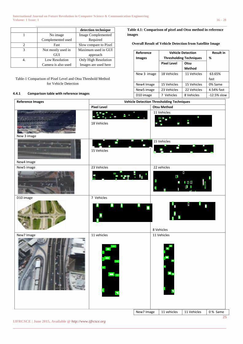
Table 1 show the comparison between pixel level and Otsu

method which we used in this proposed work.

Table 2 shows that in the new 3 image when we calculates

the vehicles from pixel level thresholding method it

calculated 18 vehicles and when we calculate from Otsu

method then it calculate 11 vehicles. So it works 63.65%

faster.

In the image new 4 image when we calculates the vehicles

from pixel level thresholding method it calculated 15 vehicles

and when we calculate from Otsu method then it calculate

15 vehicles. So it works same.

.

In the image new 5 when we calculates the vehicles from

pixel level thresholding method it calculated 23 vehicles and

when we calculate from Otsu method then it calculate 22

vehicles. So it works 4.54% faster.

In the image D10 when we calculates the vehicles from pixel

level thresholding method it calculated 7 vehicles and when

we calculate from Otsu method then it calculate 8 vehicles.

So it works 12.5 % slower.

In the image new 7 when we calculates the vehicles from

pixel level thresholding method it calculated 11 vehicles and

when we calculate from Otsu method then it calculate 11

vehicles. So it works same.

The overall result shows that pixel level thresholding method

is faster than Otsu thresholding method.

Sr. No Pixel level

(This Method)

Otsu Method

Previous vehicle

0

1000

2000

3000

4000

5000

6000

7000

8000


0 50 100 150 200 250

0

500

1000

1500

2000

2500

3000

3500

4000

4500


0 50 100 150 200 250

0

500

1000

1500

2000

2500

3000

3500


0 50 100 150 200 250



_____________________________________________________________________________________


detection technique

1 No image

Complemented used

Image Complemented

Required

2 Fast Slow compare to Pixel

3 Not mostly used in

GUI

Maximum used in GUI

approach

4. Low Resolution

Camera is also used

Only High Resolution

Images are used here

Table-1 Comparison of Pixel Level and Otsu Threshold Method

for Vehicle Detection

4.4.1 Comparison table with reference images

Table 4.1: Comparison of pixel and Otsu method in reference

images

Overall Result of Vehicle Detection from Satellite Image

Reference

Images

Vehicle Detection

Thresholding Techniques

Result in

%

Pixel Level Otsu

Method

New 3 image 18 Vehicles 11 Vehicles 63.65%

fast

New4 Image 15 Vehicles 15 Vehicles 0% Same

New5 image 23 Vehicles 22 Vehicles 4.54% fast

D10 image 7 Vehicles 8 Vehicles -12.5% slow

New7 Image 11 vehicles 11 Vehicles 0 % Same

Reference Images Vehicle Detection Thresholding Techniques

Pixel Level Otsu Method

New 3 image

18 Vehicles

11 Vehicles

New4 Image

15 Vehicles

15 Vehicles

New5 image

23 Vehicles

22 vehicles

D10 image

7 Vehicles

8 Vehicles

New7 Image

11 vehicles

11 Vehicles



_____________________________________________________________________________________


Table 2: comparison of pixel level and Otsu method in

percentage

% faster/slowe calculation = (pixel level thresholding-Otsu

Method)/Otsu Method

Overall Average among 5 Images would be 11.138%

Overall System Average = New3+New4+New5+D10+New7/5

Overall System Average = 63.65+0+4.54+ (- 12.5)+0/5

Pixel level Thresholding Overall System Average = 11.138%

Our Research says that pixel level threholding method is faster

than the Otsu method.

4.4.2 Profiler Time of Otsu Level Threholding

Figure 4.25: Profile time of Otsu level Thresholding

4.4.3 Profiler Time of Pixel Level Threholding:

Figure 4.26: Profile time of Pixel level Thresholding

5.1 Conclusion

By the time the numbers of vehicles and traffic have been

increasing day by day. With this increase, it is becoming harder to

track each vehicle for the purpose of traffic management and law

enforcement. Thus, a type of system is required, which is capable

of give appropriate solutions to the traffic issues and hence this

Vehicle detection from satellite image is developed using

morphological recognition algorithm in MATLAB and this thesis

compare two thresholding techniques to get the best result.

Morphological recognition algorithms are used to develop an

automated system in MATLAB R2013a. In which satellite images

are taken as input and converted into gray scale image for pre-

processing. After conversion these images are converted into

binary images after image complement. After conversion canny

edge detection method has done and passed this detection to the

dilation process. The area is selected after filtration and dilation

where number of vehicles is maximum and vehicles are recognized

from the image in the form of bounding box. The number of

vehicles is counted by blob analysis. Here we compare two

algorithms like pixel thresholding and Otsu thresholding method.

According to our result Pixel level thresholding is better than Otsu

method. Here image complementation are not used which make

system more powerful and make system highly applicable. The

result concluded that pixel level thresholding is better than Otsu

method for detecting the vehicles from satellite imaginary.

5.2 Future Scope

This approach makes easier to detect vehicles from

stationary images, but for moving cars or vehicles this

method will not be applicable, therefore this problem

can also be overcome in near future in order to get

more appropriate consequences.

The effect of light on vehicles reduces accuracy when

this approach is applied, so there is some scope to

improvement here.

REFERENCE

[1] S.Jayalakshmi, M.Sundaresan, "A Study of Iris

Segmentation Methods using Fuzzy CMeans and K-

Means Clustering Algorithm", International Journal of

Computer Applications (0975 – 8887) Volume 85 – No

11, January 2014.

[2] http://elearning.vtu.ac.in/17/e-Notes/DIP/Unit1-SH.pdf.

[3] Megha Soni,Anand Khare, Asst. Prof. Saurabh Jain, "A

SURVAY OF DIGITAL IMAGE PROCESSING AND ITS

PROBLEM", International Journal of Scientific and

Research Publications, Volume 4, Issue 2, February 2014

1 ISSN 2250-3153..

[4] http://folk.uio.no/walmann/Publications/PhD/node36.h

tml.

[5] Yugha R1, Dr S Uma, Swarnalatha S, Poovizhi.M,

"Multilevel Authentication System For Providing

Security", IPASJ International Journal of Computer

Science (IIJCS), Volume 3, Issue 3, March 2015.

[6] http://www.wisegeek.org/what-is-image-

processing.htm.

[7] http://www.ncsa.illinois.edu/People/kindr/phd/PART1.P

DF.

[8] K. Sumithra, S. Buvana, R. Somasundaram, "A Survey on

Various Types of Image Processing Technique",

International Journal of Engineering Research &

Technology (IJERT) Vol. 4 Issue 03, March-2015.

[9] Ian Darwin, Valerie Quercia and Tim O’Reilly, "X Window

System User’s Guide", March, 1995.

[10] "Digital Image Processing" book, By Rafael C Gonzalez,

page no. 29.

[11] http://shodhganga.inflibnet.ac.in/bitstream/10603/826

9/9/09_chapter%201.pdf. Page no. 1-4.

http://shodhganga.inflibnet.ac.in/bitstream/10603/8269/9/09_chapter%201.pdf

http://shodhganga.inflibnet.ac.in/bitstream/10603/8269/9/09_chapter%201.pdf



_____________________________________________________________________________________


[12] By Carolyn Asbury, "Brain Imaging Technologies and

Their Applications in Neuroscience".

[13] http://fas.org/irp/imint/docs/rst/Intro/Part2_1.html.

[14] http://bookboon.com/en/digital-image-processing-part-

one-ebook.

[15] Rafael C. Gonzalez, Richard E. Woods, "Digital Image

Processing Third Edition". 2008 by Pearson Education,

Inc.

[16] Ramya R, Anand Kumar S, Krinish N K, Suraj V, "Simulink

Component Recognition Using Image Processing",

International Journal of Scientific & Technology

Research Volume 4, Issue 02, February 2015.

[17] AMALOPRAVAM.G,HARISH NAIK T,JYOTI KUMARI,

"Transformation of Digital Images using Morphlogical

Operations", ISSN: 2278-9669, January 2013

(http://ijcsit.org)..

[18] e-Study Guide for: Artificial Intelligence by Stuart

Russell, ISBN 9780136042594,By Cram101 Textbook

Reviews.

[19] Trapti Sahu, Shabahat Hasan, "A Neural Network Based

Image Abstraction Technique", www.ijset.com, Volume

No.1, Issue No.2 pg:143-147, 01 April 2012..

[20] http://www.uptu.ac.in/pdf/sub_ecs_702_30sep14.pdf

(Notes Subject: Digital Image Processing Subject Code:

Ecs-70) Asst. Prof. Neeti Chadha CSE Department,

AKGEC Gzb page no. 5, 6.

[21] Naoko Evans, "Automated Vehicle Detection and

Classification using Acoustic and Seismic Signals",

September, 2010, page no.40-47.

[22] Ozcanli Ozbay, Ozge Can, "Recognition of Vehicles as

Changes in Satellite Imagery", 2010.

[23] "Remote sensing imagery in vegetation mapping: a

review" Plant Ecol (2008) 1 (1): 9-23. doi:

10.1093/jpe/rtm005..

[24] T. Blaschke, "Object based image analysis for remote

sensing", ISPRS Journal of Photogrammetry and Remote

Sensing, Volume 65, Issue 1, January 2010, Pages 2–16.

[25] Christof Ridder, Olaf Munkelt, and Harald Kirchner,

"Adaptive background estimation and foreground

detection using Kalman-filtering," in Proceedings of

International Conference on Recent Advances in

Mechatronics, 1995.

[26] S Huwer and H Niemann, "Adaptive change detection

for real-time surveillanace applications," Visual

Surveillance, 2000.

[27] T Kanade, R Collins, A Lipton, P Burt, and L Wixson,

"Advances in cooperative multi-sensor video

surveillance," in Proceedings of DARPA Image

Understanding Workshop, vol. 1, 1998.

[28] Chris Stauffer and W E Grimson, "Adaptive background

mixture models for real time tracking," in Proceedings of

IEEE Conf. on Computer Vision and Pattern Recognition

(CVPR)., vol. 2, 1999, pp. 246-252.

[29] Richard O Duda, Peter E Hart, and David G Stork, Pattern

Classification.: Wiley-Interscience, 2001.

[30] Oscar Firschein and Thomas M Strat, RADIUS: Image

Understanding for Imagery Intelligence.: Morgan

Kaufmann, 1997.

[31] Andres Huertas and Ramakant Nevatia, "Detecting

changes in aerial views of man-made structures," in

Proc. of International Conference on Computer Vision,

1998.

[32] Aaron J Heller, Yvan G Leclerc, and Quang-Tuan Luong,

"A framework for robust 3-d change detection," in

Proceedings for International Symposium on Remote

Sensing, SPIE., 2001.

[33] Richard I Hartley and Tushar Saxena, "The cubic rational

polynomial camera model," in DARPA Image

Understanding Workshop, 1997.

[34] Thomas Pollard, Ibrahim Eden, Joseph L Mundy, and

David Cooper, "A Volumetric Approach to Change

Detection in Satellite Images," Photogrammetric

Engineering and Remote Sensing, vol. 75, no. 12, p. to

appear, December 2009.

[35] Thomas Pollard, Comprehensive 3-d change detection

using volumetric appearance modeling, 2008.

[36] Gonzalez, R., and Woods, R., Digital Image

Processing, second edition, Prentice Hall, 2002.

[37] Lizhu Xie, Liying Wei, “Research on Vehicle Detection in

High Resolution Satellite Images”, 2013 Fourth Global

Congress on Intelligent Systems.

[38] X. Yang, G. A. Tang, F. D. Deng, EDARS Experiment

Tutorial of Remote Sensing Image Processing. Beijing,

CHN: Science press, 2009.

[39] X. L. Tian, “An Algorithm Based on the Satellite for Image

Enhancement,” COMPUTER KNOWLEDGE AND

TECHNOLOGY, vol. 11, pp. 315–317, Feb. 2008.

[40] Bhabatosh Chanda and Dwijest Dutta Majumder, 2002,

Digital Image Processing and Analysis.

[41] http://elearning.vtu.ac.in/17/e-

Notes/DIP/Unit%205%20&%206%20-%20SH.pdf.

[42] Otsu, Nobuyuki, “A threshold selection method from

gray-level histograms”, IEEE transactions on systems,

man, and cybernetics, vol. SMC9, no.1, January 1979,

pp.62-66

[43] The MathWorks, Inc., Image Processing Toolbox, URL:

http://www.mathworks.com/access/helpdesk/help/tool

box/images/

[44] Lizhu Xie, Liying Wei. “Research on Vehicle Detection in

High Resolution Satellite Images”, 2013 Fourth Global

Congress on Intelligent Systems.

[45] Sumalatha Kuthadi, “DETECTION OF OBJECTS FROM

HIGH-RESOLUTION SATELLITE IMAGES", May 2005, page

no. 5-10.

[46] Rocio Alba-Flores, "Evaluation of the Use of High-

Resolution Satellite Imagery in Transportation

Applications", August 2005, page no. 18-22.

[47] http://www.eecs.berkeley.edu/~fateman/kathey/node3

.html.

[48] http://en.wikipedia.org/wiki/K-means_clustering.

http://elearning.vtu.ac.in/17/e-Notes/DIP/Unit%205%20&%206%20-%20SH.pdf

http://elearning.vtu.ac.in/17/e-Notes/DIP/Unit%205%20&%206%20-%20SH.pdf

http://www.mathworks.com/access/helpdesk/help/toolbox/images/

http://www.mathworks.com/access/helpdesk/help/toolbox/images/

http://www.eecs.berkeley.edu/~fateman/kathey/node3.html

http://www.eecs.berkeley.edu/~fateman/kathey/node3.html



_____________________________________________________________________________________


automatic vehicle detection using various object …1.4 image processing with mathcad and matlab....

Documents