automatic speech recognition: human computer interface for kinyarwanda language

AUTOMATIC SPEECH RECOGNITION:HUMAN COMPUTER INTERFACE FOR

KINYARWANDA LANGUAGE

Muhirwe Jackson

BSc (Mak)

A Project Report Submitted in Partial Fulfilment of the

Requirements for the Award of the DegreeMaster of Science in Computer Science of

Makerere University

August 2005

Title page

i

DECLARATION

I, Muhirwe Jackson, do hereby declare this project report as my original work and has neverbeen submitted for any award of a degree in any institution of higher learning.

Signed: .......................................................... Date: ...........................................Muhirwe Jackson,Candidate.

ii

APPROVAL

This report has been submitted for examination with my approval as supervisor.

Signed: .......................................................... Date: ...........................................Dr. Jehopio Peter, Ph.D.Supervisor.

iii

DEDICATION

To the prince of peace, my Lord and savior Jesus ChristLet it be said of me that my source of strength is Christ alone.

To my wife, Yvonne Muhirwewho has greatly encouraged and supported me during my studies.

To my children:who always bring joy to my life.

To my mum: Ms Mukankuliza JoyceWho has wonderfully supported and encouraged throughout my education: There’s no

mother like you.

To my Brothers and sisterI love you all

iv

”I can do all things through Christwhich strengtheneth me.” Phil 4:13KJV

v

ACKNOWLEDGEMENT

Success in life is never attained single handedly. I would like to express my heartfelt grati-tude to my God almighty who revealed Himself to me through the Holy spirit and has sincebeen my source of strength and wisdom. I wish to extend thanks to my supervisor, Dr.Peter Jehopio for the professional guidance that has enabled me accomplish this research.I also wish to extend my sincere thanks to the dean Faculty of computing and Informationtechnology Dr. Baryamureeba Venansius for all the support he has provided to me bothmorally and financially without which this project may not have been a success.I would like to appreciate my wife, Yvonne Muhirwe for being such a wonderful, loving andunderstanding wife. Thanks for giving me space and time to dedicate to my studies, mysuccess is your success.I extend my thanks and appreciation to the Rector of the Kigali Institute of Education, Mr.Mudidi Emmanuel for having faith in me and for all the support he provided to me at thebeginning of the course. I extend my thanks and appreciation to the Rwandan Governmentthrough the Student Financing Agency for Rwanda (SFAR) for sponsoring me for the entirecourse.My sincere appreciation goes to Makerere University Faculty of computing and InformationTechnology staff, more especially Paul Bagenda, and Kanagwa Ben for their technical sup-port.

Lastly but not least, I acknowledge all my lecturers and all my classmates on the computerscience programmes for having made my academic and social life comfortable at MakerereUniversity.

MAY GOD BLESS YOU ABUNDANTLY

vi

LIST OFACRONYMS/ABBREVIATIONS

LVCSR Large Vocabulary Continuous Speech Recognition.

ASR Automatic speech recognition

TTS Text-to-speech

IVR Interactive Voice Response

HCI Human Computer Interaction

I/O Input and Output

SU Speech Understanding

GUI Graphical User Interface

DVI Direct Voice Input

HMM Hidden Markov Models

HTK Hidden Markov Model Toolkit.

BNF Backus-Naur form

SLF Standard Lattice Format

MLF Master Label Files

MFCC Mel Frequency Cepstral Coefficients.

vii

Contents

TITLE PAGE . . . . . . . . . . . . . . . . . . . . . . . . . . . . . . . . . . . . . . i

DECLARATION . . . . . . . . . . . . . . . . . . . . . . . . . . . . . . . . . . . . ii

APPROVAL . . . . . . . . . . . . . . . . . . . . . . . . . . . . . . . . . . . . . . . iii

DEDICATION . . . . . . . . . . . . . . . . . . . . . . . . . . . . . . . . . . . . . iv

ACKNOWLEDGEMENT . . . . . . . . . . . . . . . . . . . . . . . . . . . . . . . vi

LIST OF ACRONYMS/ABBREVIATIONS . . . . . . . . . . . . . . . . . . . . . vii

LIST OF FIGURES . . . . . . . . . . . . . . . . . . . . . . . . . . . . . . . . . . xi

ABSTRACT . . . . . . . . . . . . . . . . . . . . . . . . . . . . . . . . . . . . . . xii

1 INTRODUCTION 1

1.1 Background to the Study . . . . . . . . . . . . . . . . . . . . . . . . . . . . . 1

1.2 Statement of the Problem . . . . . . . . . . . . . . . . . . . . . . . . . . . . 3

1.3 Objectives of the Study . . . . . . . . . . . . . . . . . . . . . . . . . . . . . . 3

1.3.1 General Objective . . . . . . . . . . . . . . . . . . . . . . . . . . . . . 3

1.3.2 Specific Objectives . . . . . . . . . . . . . . . . . . . . . . . . . . . . 3

1.4 Scope . . . . . . . . . . . . . . . . . . . . . . . . . . . . . . . . . . . . . . . 4

1.5 Significance of the Study . . . . . . . . . . . . . . . . . . . . . . . . . . . . . 4

2 Literature Review 6

2.1 Current State of ASR Technology and its Implications for Design . . . . . . 6

2.2 Types of ASR . . . . . . . . . . . . . . . . . . . . . . . . . . . . . . . . . . . 8

2.3 Speech Recognition Techniques . . . . . . . . . . . . . . . . . . . . . . . . . 9

2.4 Matching Techniques . . . . . . . . . . . . . . . . . . . . . . . . . . . . . . . 10

viii

2.5 Corpora . . . . . . . . . . . . . . . . . . . . . . . . . . . . . . . . . . . . . . 11

2.6 Problems in Designing Speech Recognition Systems . . . . . . . . . . . . . . 11

2.7 Similar Projects Carried out . . . . . . . . . . . . . . . . . . . . . . . . . . . 12

3 METHODOLOGY 14

3.1 Data Preparation . . . . . . . . . . . . . . . . . . . . . . . . . . . . . . . . . 16

3.1.1 The Task Grammar . . . . . . . . . . . . . . . . . . . . . . . . . . . . 16

3.1.2 A Pronunciation Dictionary . . . . . . . . . . . . . . . . . . . . . . . 18

3.1.3 Recording . . . . . . . . . . . . . . . . . . . . . . . . . . . . . . . . . 19

3.1.4 Phonetic Transcription . . . . . . . . . . . . . . . . . . . . . . . . . . 21

3.1.5 Encoding the Data . . . . . . . . . . . . . . . . . . . . . . . . . . . . 22

3.2 Parameter Estimation (Training) . . . . . . . . . . . . . . . . . . . . . . . . 23

3.2.1 Training Strategies . . . . . . . . . . . . . . . . . . . . . . . . . . . . 23

3.2.2 HMM Definition. . . . . . . . . . . . . . . . . . . . . . . . . . . . . . 25

3.2.3 HMM Training . . . . . . . . . . . . . . . . . . . . . . . . . . . . . . 27

3.2.4 Training . . . . . . . . . . . . . . . . . . . . . . . . . . . . . . . . . . 29

3.3 Recognition . . . . . . . . . . . . . . . . . . . . . . . . . . . . . . . . . . . . 29

3.4 Running the Recognizer Live . . . . . . . . . . . . . . . . . . . . . . . . . . . 31

4 RESULTS 32

4.1 Perfomance Test . . . . . . . . . . . . . . . . . . . . . . . . . . . . . . . . . 32

4.2 Perfomance Analysis . . . . . . . . . . . . . . . . . . . . . . . . . . . . . . . 32

4.3 Testing the System on Live Data . . . . . . . . . . . . . . . . . . . . . . . . 33

5 DISCUSSION, CONCLUSION AND RECOMMENDATIONS 35

5.1 Discussion . . . . . . . . . . . . . . . . . . . . . . . . . . . . . . . . . . . . . 35

5.2 Conclusion . . . . . . . . . . . . . . . . . . . . . . . . . . . . . . . . . . . . . 37

5.3 Areas for Further Study . . . . . . . . . . . . . . . . . . . . . . . . . . . . . 37

REFERENCES 39

ix

APPENDICES 43

Appendix A: Word Network . . . . . . . . . . . . . . . . . . . . . . . . . . . . . . 43

Appendix B: Training Sentences . . . . . . . . . . . . . . . . . . . . . . . . . . . . 45

Appendix C: Master Label Files . . . . . . . . . . . . . . . . . . . . . . . . . . . . 47

Appendix D: Training Data . . . . . . . . . . . . . . . . . . . . . . . . . . . . . . 62

Appendix E: HMM Definitions . . . . . . . . . . . . . . . . . . . . . . . . . . . . 67

Appendix F: VarFloor1 . . . . . . . . . . . . . . . . . . . . . . . . . . . . . . . . . 81

Appendix G: Recognition Output . . . . . . . . . . . . . . . . . . . . . . . . . . . 82

Appendix H: Testing Data . . . . . . . . . . . . . . . . . . . . . . . . . . . . . . . 86

x

List of Figures

3.1 Components of an ASR system . . . . . . . . . . . . . . . . . . . . . . . . . 15

3.2 Grammar for voice dialling . . . . . . . . . . . . . . . . . . . . . . . . . . . . 17

3.3 Process of creating a word lattice . . . . . . . . . . . . . . . . . . . . . . . . 17

3.4 Recording and labelling data using hslab . . . . . . . . . . . . . . . . . . . . 20

3.5 Training HMMs . . . . . . . . . . . . . . . . . . . . . . . . . . . . . . . . . . 24

3.6 Training isolated whole word models . . . . . . . . . . . . . . . . . . . . . . 25

3.7 HMM training process . . . . . . . . . . . . . . . . . . . . . . . . . . . . . . 27

3.8 Speech recognition process . . . . . . . . . . . . . . . . . . . . . . . . . . . . 30

4.1 Speech recognition results . . . . . . . . . . . . . . . . . . . . . . . . . . . . 33

4.2 Live data recognition results . . . . . . . . . . . . . . . . . . . . . . . . . . . 34

xi

ABSTRACT

The main purpose of the study was to develop an automatic speech recogniser for Kin-

yarwanda language. The products of the study include an automatic phone dialling speech

corpus, a Kinyarwanda digit speech recogniser, a recipe for building HMM speech recognis-

ers, especially for Kinyarwanda language.

Two different corpora were collected of audio recordings of indigenous Kinyarwanda lan-

guage speakers, in which subjects read aloud numeric digits. One of the collected corpora

contained the trainig data and the other the testing data.

The system was implemented using the HMM toolkit HTK by training HMMs of the words

making the vocabulary on the training data. The trained system was tested on data other

than the training data and results revealed that 94.47% of the tested data were correctly

recognized.

The developed system can be used by developers and researchers interested in speech recog-

nition for Kinyarwanda language and any other related African language. The findings

of the study can be generalized to cater for large vocabularies and for continuous speech

recognition.

xii

Chapter 1

INTRODUCTION

1.1 Background to the Study

Speech is one of the oldest and most natural means of information exchange between human

beings. We as humans speak and listen to each other in human-human interface. For

centuries people have tried to develop machines that can understand and produce speech

as humans do so naturally (Pinker, 1994 [20]; Deshmukh et al., 1999 [5]). Obviously such

an interface would yield great benefits (Kandasamy,1995,) [12]. Attempts have been made

to develop vocally interactive computers to realise voice/speech recognition. In this case a

computer can recognize text and give out a speech output (Kandasamy,1995) [12].

Voice/speech recognition is a field of computer science that deals with designing computer

systems that recognize spoken words. It is a technology that allows a computer to identify

the words that a person speaks into a microphone or telephone.

Speech recognition can be defined as the process of converting an acoustic signal, captured

by a microphone or a telephone, to a set of words (Zue et al., 1996 [36]; Mengjie, 2001 [17]).

Automatic speech recognition (ASR) is one of the fastest developing fields in the framework of

speech science and engineering. As the new generation of computing technology, it comes as

the next major innovation in man-machine interaction, after functionality of text-to-speech

(TTS), supporting interactive voice response (IVR) systems.

The first attempts (during the 1950s) to develop techniques in ASR, which were based on

the direct conversion of speech signal into a sequence of phoneme-like units, failed. The

1

first positive results of spoken word recognition came into existence in the 1970s, when gen-

eral pattern matching techniques were introduced. As the extension of their applications

was limited, the statistical approach to ASR started to be investigated, at the same period.

Nowadays, the statistical techniques prevail over ASR applications. Common speech recog-

nition systems these days can recognize thousands of words. The last decade has witnessed

dramatic improvement in speech recognition technology, to the extent that high performance

algorithms and systems are becoming available. In some cases, the transition from labora-

tory demonstration to commercial deployment has already begun (Zue et al., 1996) [36]. The

reason for the evolution of ASR, hence improved is that it has a lot of applications in many

aspects of our daily life, for example, telephone applications, applications for the physically

handicapped and illiterates and many others in the area of computer science. Speech recog-

nition is considered as an input as well as an output during the Human Computer Interaction

(HCI) design . HCI involves the design implementation and evaluation of interactive systems

in the context of the users’ task and work.(Dix et al., 1998) [6].

The list of applications of automatic speech recognition is so long and is growing; some

of known applications include virtual reality, Multimedia searches, auto-attendants, travel

information and reservation, translators, natural language understanding and many more

applications (Scansoft, 2004 [27]; Robertson, 1998 [24]).

Speech technology is the technology of today and tomorrow with a developing number of

methods and tools for better implementation. Speech recognition has a number of practical

implementations for both fun and serious works. Automatic speech recognition has an

interesting and useful implementation in expert systems, a technology whereby computers

can act as a substitute for a human expert. An intelligent computer that acts, responds or

thinks like a human being can be equipped with an automatic speech recognition module

that enables it to process spoken information. Medical diagnostic systems, for example, can

diagnose a patient by asking him a set of questions, the patient responding with answers,

and the system responds with what might be a possible disease.

2

1.2 Statement of the Problem

As the use of ICT tools, especially the computer, is becoming inevitable, there are many

Rwandans who are left out due to inadequate human computer interface (HCI) design con-

siderations. A case in point is the many Rwandans who are left out due to language barrier

(Earth trends, 2003) [8]. These people can only read and write in their mother-tongue,

Kinyarwanda language making it impossible for them to use ICT conventional tools that are

built in the two International languages, English and French used in Rwanda.

The purpose of this project was therefore to design and train a speech recognition system

that could be used by application developers to develop application that will take indige-

nous Kinyarwanda language speakers aboard the current information and communication

technologies to fast-track the benefits of ICT.

1.3 Objectives of the Study

1.3.1 General Objective

The general objective of the project was to develop an automatic speech recogniser for

Kinyarwanda language.

1.3.2 Specific Objectives

The specific objectives of the project are:

i. To critically review literature related to ASR.

ii. To identify speech corpus elements exhibited in African languages such as Kinyarwanda

language.

iii. To build a Kinyarwanda language speech corpus for a voice operated telephone system.

iv. To implement an isolated whole word speech recognizer that is capable of recognizing

and responding to speech.

3

v. To train the above developed system in order to make it speaker independent.

vi. To validate the automatic speech recognizer developed during the study.

1.4 Scope

The project was limited to only isolated whole words and trained and tested on only one

(1) word sentences consisting of the numeric digit 0 to 9 that could be used on operating a

voice operated telephone system.

Human speech is inherently a multi modal process that involves the analysis of the uttered

acoustic signal and includes higher level knowledge sources such as grammar semantics and

pragmatics (Dupont, 2000) [7]. This research intends to focus only on the acoustic signal

processing ignoring the visual input.

1.5 Significance of the Study

The proposed research has theoretical, practical, and methodological significance:

i. The speech corpus developed will be very useful to any researcher who may wish to

venture into Kinyarwanda language automatic speech recognition.

ii. By developing and training a speech recognition system in Kinyarwanda language, the

semi illiterates would be able to use it in accessing IT tools. This would help bridge

the digital divide, since Rwanda is a monolingual nation with a population of about

8Million (Earth trends, 2003) [8] all speaking Kinyarwanda language.

iii. Since Speech technology is the technology of today and tomorrow, the results of this

research will help many indigenous Kinyarwanda language speakers who are scattered

all over the great lakes region to take advantage of the many benefits of ICT.

iv. The technology will find applicability in systems such as banking, telecommunications,

transport, Internet portals, accessing PC, emailing, administrative and public services,

cultural centres and many others.

4

v. The built system will be very useful to computer manufactures and software developers

as they will have a speech recognition engine to include Kinyarwanda language in their

applications.

vi. By developing and training a speech recognition system in Kinyarwanda language, it

would mark the first step towards making ICT tools become more usable by the blind

and elderly people with seeing disabilities.

5

Chapter 2

Literature Review

Human computer interactions as defined in the background is concerned about ways Users

(humans) interact with the computers. Some users can interact with the computer using the

traditional methods of a keyboard and mouse as the main input devices and the monitor

as the main output device. Due to one reason or another some users cannot be able to

interact with machines using a mouse and keyboard (Rudnicky et al., 1993) [26] device,

hence the need for special devices. Speech recognition systems help users who in one way

or the other can not be able to use the traditional Input and Output(I/O) devices. For

about four decades human beings have been dreaming of an ”intelligent machine” which

can master the natural speech (Picheny, 2002) [19]. In its simplest form, this machine

should consist of two subsystems, namely automatic speech recognition (ASR) and speech

understanding (SU) (Reddy, 1976) [23]. The goal of ASR is to transcribe natural speech

while SU is to understand the meaning of the transcription. Recognizing and understanding

a spoken sentence is obviously a knowledge-intensive process, which must take into account

all variable information about the speech communication process, from acoustics to semantics

and pragmatics.

2.1 Current State of ASR Technology and its Implica-

tions for Design

The design of user interfaces for speech-based applications is dominated by the underlying

ASR technology. More often than not, design decisions are based more on the kind of recog-

6

nition the technology can support rather than on the best dialogue for the user (Mane et

al., 1996) [16]. The type of design will depend, broadly, on the answer to this question:

What type of speech input can the system handle, and when can it handle it? When isolated

words are all the recognizer can handle, then the success of the application will depend on the

ability of designers to construct dialogues that lead the user to respond using single words.

Word spotting and the ability to support more complex grammars opens up additional flex-

ibility in the design, but can make the design more difficult by allowing a more diverse set

of responses from the user. Some current systems allow a limited form of natural language

input, but only within a very specific domain at any particular point in the interaction.

Even in these cases, the prompts must constrain the natural language within acceptable

bounds. No systems allow unconstrained natural language interaction, and it’s important

to note that most human-human transactions over the phone do not permit unconstrained

natural language either. Typically, a customer service representative will structure the con-

versation by asking a series of questions.

With ”barge-in” (also called ”cut-through”) (Mane et al., 1996,) [16], a caller can interrupt

prompts and the system will still be able to process the speech, although recognition per-

formance will generally be lower. This obviously has a dramatic influence on the prompt

design, because when barge-in is available it’s possible to write longer more informative

prompts and let experienced users barge-in. Interruptions are very common in human-

human conversations, and in many applications, designers have found that without barge-in

people often have problems. There are a variety of situations, however, in which it may not

be possible to implement barge-in. In these cases, it is still usually possible to implement

successful applications, but particular care must be taken in the dialogue design and error

messages. Another situation in which technology influences design involves error recovery.

It is especially frustrating when a system makes the same mistake twice, but when the active

vocabulary can be updated dynamically, recognizer choices that have not been confirmed can

be eliminated, and the recognizer will never make the same mistake twice. Also, when more

than one choice is available (this is not always the case, as some recognizers return only the

top choice), then after the top choice is disconfirmed, the second choice can be presented.

7

2.2 Types of ASR

ASR products have existed in the marketplace since the 1970s. However, early systems

were expensive hardware devices that could only recognize a few isolated words (i.e. words

with pauses between them), and needed to be trained by users repeating each of the vo-

cabulary words several times. The 1980s and 90s witnessed a substantial improvement in

ASR algorithms and products, and the technology developed to the point where, in the late

1990s, software for desktop dictation became available ’off-the-shelf’ for only a few tens of

dollars. From a technological perspective it is possible to distinguish between two broad

types of ASR: ’direct voice input’ (DVI) and ’large vocabulary continuous speech recogni-

tion’ (LVCSR). DVI devices are primarily aimed at voice command-and-control, whereas

LVCSR systems are used for form filling or voice-based document creation. In both cases

the underlying technology is more or less the same. DVI systems are typically configured

for small to medium sized vocabularies (up to several thousand words) and might employ

word or phrase spotting techniques. Also, DVI systems are usually required to respond im-

mediately to a voice command. LVCSR systems involve vocabularies of perhaps hundreds

of thousands of words, and are typically configured to transcribe continuous speech. Also,

LVCSR need not be performed in real-time - for example, at least one vendor has offered a

telephone-based dictation service in which the transcribed document is e-mailed back to the

user.

Specific examples of application of ASR may include but not limited to the following

i. large vocabulary dictation - for RSI sufferers and quadriplegics, and for formal docu-

ment preparation in legal or medical services.

ii. Interactive voice response - for callers who do not have tone pads, for the automation

of call centers, and for access to information services such as stock market quotes.

iii. Telecom assistants - for repertory dialling and personal management systems.

iv. Process and factory management - for stocktaking, measurement and quality control.

8

2.3 Speech Recognition Techniques

Speech recognition techniques are the following:

i. Template based approaches matching (Rabiner et al., 1979) [22], Unknown speech is

compared against a set of pre-recorded words( templates) in order to find the best

match. This has the advantage of using perfectly accurate word models. But it also

has the disadvantage that pre-recorded templates are fixed, so variations in speech

can only be modelled by using many templates per word, which eventually becomes

impractical. Dynamic time warping is such a typical approach (Tolba et al., 2001) [31].

In this approach, the templates usually consists of representative sequences of features

vectors for corresponding words. The basic idea here is to align the utterance to each of

the template words and then select the word or word sequence that contains the best.

For each utterance , the distance between the template and the observed feature vectors

are computed using some distance measure and these local distances are accumulated

along each possible alignment path. The lowest scoring path then identifies the optimal

alignment for a word and the word template obtaining the lowest overall score depicts

the recognised word or sequence of words.

ii. Knowledge based approaches: An expert knowledge about variations in speech is hand

coded into a system. This has the advantage of explicit modelling variations in speech;

but unfortunately such expert knowledge is difficult to obtain and use successfully.

Thus this approach was judged to be impractical and automatic learning procedure

was sought instead.

iii. Statistical based approaches. In which variations in speech are modelled statistically,

using automatic, statistical learning procedure, typically the Hidden Markov Models,

or HMM. The approach represent the current state of the art. The main disadvantage

of statistical models is that they must take priori modelling assumptions which are

liable to be inaccurate, handicapping the system performance. In recent years, a new

approach to the challenging problem of conversational speech recognition has emerged,

holding a promise to overcome some fundamental limitations of the conventional Hid-

den Markov Model (HMM) approach (Bridle et al., 1998 [2]; Ma and Deng, 2004 [14]).

9

This new approach is a radical departure from the current HMM-based statistical mod-

eling approaches. Rather than using a large number of unstructured Gaussian mixture

components to account for the tremendous variation in the observable acoustic data of

highly coarticulated spontaneous speech, the new speech model that (Ma and Deng,

2004) [15] have developed provides a rich structure for the partially observed (hidden)

dynamics in the domain of vocal-tractresonances.

iv. Learning based approaches. To overcome the disadvantage of the HMMs machine

learning methods could be introduced such as neural networks and genetic algorithm/

programming. In those machine learning models explicit rules or other domain expert

knowledge) do not need to be given they a can be learned automatically through

emulations or evolutionary process.

v. The artificial intelligence approach attempts to mechanise the recognition procedure

according to the way a person applies its intelligence in visualizing, analysing, and

finally making a decision on the measured acoustic features. Expert system are used

widely in this approach (Mori et al., 1987) [18]

2.4 Matching Techniques

Speech-recognition engines match a detected word to a known word using one of the following

techniques (Svendsen et al., 1989) [29].

i. Whole-word matching. The engine compares the incoming digital-audio signal against

a prerecorded template of the word. This technique takes much less processing than

sub-word matching, but it requires that the user (or someone) prerecord every word

that will be recognized - sometimes several hundred thousand words. Whole-word

templates also require large amounts of storage (between 50 and 512 bytes per word)

and are practical only if the recognition vocabulary is known when the application is

developed.

ii. Sub-word matching. The engine looks for sub-words - usually phonemes - and then

performs further pattern recognition on those. This technique takes more processing

10

than whole-word matching, but it requires much less storage (between 5 and 20 bytes

per word). In addition, the pronunciation of the word can be guessed from English

text without requiring the user to speak the word beforehand.

(Svendsen et al., 1989) [29], (Rabiner et al., 1981) [22], and (Wilpon et al., 1988) [34] discuss

that research in the area of automatic speech recognition had been pursued for the last three

decades, only whole-word based speech recognition systems have found practical use and

have become commercial successes. Though whole word models have become a success the

researchers mentioned above all agree that they still suffer from two major problems, that

is co-articulation problems and requiring a lot of training to build a good recognizer.

2.5 Corpora

To build any speech engine whether a speech recognition engine or speech sythensis engine

you need a corpus. Corpora are any collections of text and/or speech, and are used as a

basis of statistical processing of natural language (Jurafsky and Martin, 2000) [10]. There

are various kinds of corpora: tagged or untagged; monolingual or multilingual; balanced or

specialized. For example, one of the largest and best-known corpora, the British National

Corpus (Warwick, 1997) [32], consists of 100 million words of written (about 90%) and speech

(about 10%) data collected from modern British English which covers a variety of styles and

subjects. Speech corpus could be specialised with only telephone data (Cole et al., 1992) [4],

names, names of places, etc. Developing a speech corpus may involve data collection and

transcription(Cole et al., 1994) [3].

2.6 Problems in Designing Speech Recognition Sys-

tems

ASR has been proved to be a not easy task. According to (Rudnicky et al., 1993) [26] the

main challenge in the implementation of ASR on desktops is the current existence of mature

and efficient alternatives, the keyboard and mouse. In the past years, speech researchers

have found several difficulties that contrast with the optimism of the first speech technology

11

pioneers. According to Ray Reddy (Reddy, 1976) [23] in his review of speech recognition

by machines says that the problems in designing ASR are due to the fact that it is related

to so many other fields such as acoustics, signal processing, pattern recognition, phonetics,

linguistics, psychology, neuroscience, and computer science. And all these problems can be

described according to the tasks to be performed.

i. Number of speakers: With more than one speaker, an ASR system must cope with

the difficult problem of speech variability from one speaker to another. This is usually

achieved through the use of large speech database as training data (Huang et al.,

2004) [9].

ii. Nature of the utterance: Isolated word recognition impose on the speaker the need to

insert artificial pause between successive utterances. Continuous speech recognition

systems are able to cope with natural speech utterances in which words may be tied

together and may at times be strongly affected by co articulation. Spontaneous speech

recognition systems allow the possibility of pause and false starts in the utterance, the

use of words not found in the lexicon, etc.

iii. Vocabulary size: In general, increasing the size of the vocabulary decrease the recog-

nition scores.

iv. Differences between speakers due to sex, age, accent and so on.

v. Language complexity: The task of continuous speech recognisers is simplified by limit-

ing the number of possible utterances through the imposition of syntactic and semantic

constraints.

vi. Environment conditions: The sites for real applications often present adverse conditions

(such as noise, distorted signal, and transmission line variability) which can drastically

degrade the system performance.

2.7 Similar Projects Carried out

African Speech Technology is the working title of a 3-year project promoting the development

of the official languages of South Africa through language and speech technology applications

12

at the University of Stellenbosch. So far they have covered South African English, isiZulu,

isiXhosa, Sesotho and Afrikaans (Roux et al., 2000) [25] . While African Speech Technology

and other research centers are engaged in speech technology research, there is still a long

way to go in automatic speech recognition of many indigenous languages in Africa. Most of

what is done in automatic speech recognition worldwide revolves around the many English

dialects and major languages of the northern hemisphere.

13

Chapter 3

METHODOLOGY

This chapter gives a full description of how the Kinyarwanda language speech recognition

system was developed. The goal of the project was to build a robust whole word recognizer.

That means it should be able to generalise both from speaker specific properties and its

training should be more than just instance based learning. In the HMM paradigm this is

supposed to be the case, but the researcher intended to put this into practice.

As the time scope was limited and to be able to focus on more specific issues than HMM in

general, the Hidden Markov Model toolkit (HTK) was used. HTK is a toolkit for building

Hidden Markov Models (HMMs). HMMs can be used to model any time series and the

core of HTK is similarly general-purpose. However, HTK is primarily designed for building

HMM-based speech processing tools, in particular recognisers (Young S.et al., 2002) [35].

Secondly to reduce the difficulties of the task, a very limited language model was used.

Future research can be directed to more extensive language models. In ASR systems acoustic

information is sampled as a signal suitable for processing by computers and fed into a

recognition process. The output of the system is a hypothesis transcription of the utterances.

14

Figure 3.1: Components of an ASR system

Speech recognition is a complicated task and state of the art recognition systems are very

complex. For pragmatic reasons the project was restricted to the same domain as the HTK

tutorial suggests namely instructions that a telephone can perform, ”Dial one two zero”.

System construction approach. There are a big number of different approaches for the

implementation of an ASR but for this project the four major processing steps as suggested

by HTK (Young S.et al., 2002,) [35] were considered namely data preparation, training,

Recognition/testing and analysis. For implementation purposes the following sub-processes

were taken

i. Building the task grammar

ii. Constructing a dictionary for the models

iii. Recording the data.

iv. Creating transcription files for training data

v. Encoding the data (feature processing)

vi. (Re-) training the acoustic models

vii. Evaluating the recognisers against the test data

viii. Reporting recognition results

15

3.1 Data Preparation

The first stage of any recogniser development project is data preparation. Speech data is

needed both for training and for testing. In the system built here, all of this speech was

recorded from scratch. The training data is used during the development of the system. Test

data provides the reference transcriptions against which the recogniser’s performance can be

measured and a convenient way to create them is to use the task grammar as a random

generator. In the case of the training data, the prompt scripts will be used in conjunction

with a pronunciation dictionary to provide the initial phone level transcriptions needed to

start the HMM training process.

It follows from above that before the data can be recorded, a phone set must be defined, a

dictionary must be constructed to cover both training and testing and a task grammar must

be defined.

3.1.1 The Task Grammar

The task grammar defines constraints on what the recognizer can expect as input. As the

system built provides a voice operated interface for phone dialling, it handles digit strings.

For the limited scope of this project, only a the digits 0, 1, 9 making toy grammar were

needed. The grammar was defined in BN-form, as follows: $variable defines a phrase as

anything between the subsequent = sign and the semicolon, where | stands for a logical or.

Brackets have the usual grouping function and square brackets denote optionality. The used

toy grammar was:

#

#Task grammar

#

$digit=RIMWE|KABIRI|GATATU|KANE|GATANU|GATANDATU|KARINDWI|UMUNANI|ICYENDA|ZERO;

(SENT-START[$digit] SENT-END)

The above grammar can be depicted as a network as shown below

16

Figure 3.2: Grammar for voice dialling

Word network

The above high-level representation of a task grammar is provided for user convenience. The

HTK recogniser actually requires a word network to be defined using a low level notation

called HTK Standard Lattice Format (SLF) in which each word instance and each word-to-

word transition is listed explicitly. This word network can be created automatically from the

grammar above using the HParse tool, thus assuming that the file gram contains the above

grammar, executing

HParse gram wdnet

Creates an equivalent word network in the file wdnet (appendix A) see the figure below

Figure 3.3: Process of creating a word lattice

17

The above created lattice can now be used by another HTK tool HSGen to generate random

sentences. These are the sentences that are used later for training and testing purposes.

3.1.2 A Pronunciation Dictionary

The dictionary provides an association between words used in the task grammar and the

acoustic models which may be composed of sub word (phonetic, sysllabic etc,,) units. Since

this project provides a voice operated interface the dictionary could have been constructed

by hand but the researcher wanted to try a different method which could be used to con-

struct a dictionary for a large vocabulary ASR system. In order to train the HMM network,

a large pronunciation dictionary is needed.

Since we are using whole-word models in this assignment, the dictionary has a simple struc-

ture. A file called ’lexicon’ was created with the following structure:

GATANDATU gatandatu

GATANU gatanu

GATATU gatatu

ICYENDA icyenda

KABIRI kabiri

KANE kane

KARINDWI karindwi

RIMWE rimwe

SENT-END [] sil

SENT-START [] sil

UMUNANI umunani

ZERO zero

A file named wdlist.txt was created containing all the words that make up the vocabulary.

GATANDATU

GATANU

GATATU

ICYENDA

18

KABIRI

KANE

KARINDWI

RIMWE

SENT-END

SENT-START

UMUNANI

ZERO

The dictionary was created finally by using HDman as follows

HDman -m -w wdlist.txt -n models1 -l dlog dict lexicon

This will create a new dictionary called dict by searching the source dictionary(s) lexicon to

find pronunciations for each word in wdlist.txt. Here, the wdlist.txt in question needs only

to be a sorted list of the words appearing in the task grammar given above. The option

-l instructs HDMan to output a log file dlog which contains various statistics about the

constructed dictionary. In particular, it indicates if there are words missing. HDMan can

also output a list of the words used, here called models1. Once training and test data has

been recorded, an HMM will be estimated for each of these words.

3.1.3 Recording

In order to train and test the recognizer on the domain and on the voices of some selected

people, 10 sentences were automatically generated from the grammar with HTK’s HSGen.

See appendix B for the training and testing sentences. Speech data of six (6) different

speakers 3 males and 3 females of different age groups was recorded. Due to my lack of

access to a recording studio, the recordings were done in an office on Sundays when there

are no people in the office. As the toolkit does not require phoneme duration information

for the training sentences, the (differences in) timing in the pronunciation of the training

sentences is not important. The toolkit learns to recognise the words through fitting the

word transcriptions on the training set. These transcriptions are used for all realisations of

the same sentence, even though there might be variation between speakers relative to the

transcription.

The speakers were given a list with sentences which they had to read aloud. After about 5

19

sentences they took a short break, and drank a glass of water. The training corpus consisting

of 150 sentences were recorded and labelled using the HTK tool HSLab.

Figure 3.4: Recording and labelling data using hslab

After recording and labelling the training sentences, a test corpus was also created the same

way as the training corpus but in this case 70 sentences were used for training. The differences

noted in pronunciation between speakers (and their consequences) can be categorised as

articulation variation E.g., some speakers had a rolling ‘r’, others not in, example, ‘kabiri’,

’rimwe’ Phonetic change degrades the quality of the training set, since the same phonetic

transcription was used for all speakers. These phonetic changes problems were solved by

using isolated whole word models and having many different sentences such at the end of

the day I created a speaker independent system.

Articulation variation on the other hand is of course a problem for recognition but if there

20

was no articulation variation the task of recognising would become an instance based learning

problem.

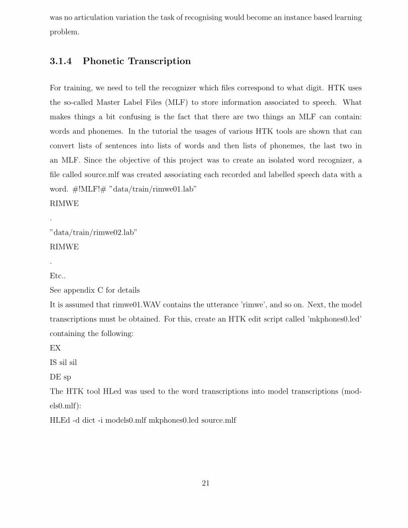
3.1.4 Phonetic Transcription

For training, we need to tell the recognizer which files correspond to what digit. HTK uses

the so-called Master Label Files (MLF) to store information associated to speech. What

makes things a bit confusing is the fact that there are two things an MLF can contain:

words and phonemes. In the tutorial the usages of various HTK tools are shown that can

convert lists of sentences into lists of words and then lists of phonemes, the last two in

an MLF. Since the objective of this project was to create an isolated word recognizer, a

file called source.mlf was created associating each recorded and labelled speech data with a

word. #!MLF!# ”data/train/rimwe01.lab”

RIMWE

.

”data/train/rimwe02.lab”

RIMWE

.

Etc..

See appendix C for details

It is assumed that rimwe01.WAV contains the utterance ’rimwe’, and so on. Next, the model

transcriptions must be obtained. For this, create an HTK edit script called ’mkphones0.led’

containing the following:

EX

IS sil sil

DE sp

The HTK tool HLed was used to the word transcriptions into model transcriptions (mod-

els0.mlf):

HLEd -d dict -i models0.mlf mkphones0.led source.mlf

21

3.1.5 Encoding the Data

The speech recognition tools cannot process directly on speech waveforms. These have to be

represented in a more compact and efficient way. This step is called ”acoustical analysis”:

The signal is segmented in successive frames (whose length is chosen between 20ms and

40ms, typically), overlapping with each other. Each frame is multiplied by a windowing

function (e.g. Hamming function).

A vector of acoustical coefficients (giving a compact representation of the spectral properties

of the frame) is extracted from each windowed frame.

In order to specify to HTK the nature of the audio data (format, sample rate, etc.) and

feature extraction parameters (type of feature, window length, pre-emphasis, etc.), a config-

uration file (config.txt) was created as follows:

#Coding parameters

SOURCEKIND = waveform

SOURCEFORMAT = HTK

SOURCERATE = 625

TARGETKIND = MFCC 0 D A

TARGETRATE = 100000.0

SAVECOMPRESSED = T

SAVEWITHCRC = T

WINDOWSIZE = 250000.0

USEHAMMING = T

PREEMCOEF = 0.97

NUMCHANS = 26

CEPLIFTER = 22

NUMCEPS = 12

ENORMALISE = F

To run a HCopy a list of each source file and its corresponding output file was created. The

first few lines look like:

data/train/rimwe01.SIG data/MFC/rimwe.MFC

data/train/rimwe02.sig data/MFC/rimwe02.MFC

data/train/rimwe03.sig data/mfc/rimwe03.mfc

22

.

.

data/train/sil10.sig data/MFC/sil10.MFC

See appendix D for details

One line for each file in the training set. This file tells HTK to extract features from each

audio file in the first column and save them to the corresponding feature file in the second

column. The command used is:

HCopy -T 1 -C config.txt -S hcopy.scp

3.2 Parameter Estimation (Training)

Defining the structure and overall form of a set of HMMs is the first step towards building

a recognizer. The second step is to estimate the parameters of the HMMs from examples of

the data sequences that they are intended to model. This process of parameter estimation is

usually called training. The topology for each of the hmm to be trained is built by writing

a prototype definition. HTK allows HMMs to be built with any desired topology. HMM

definitions can be stored externally as simple text files and hence it is possible to edit them

with any convenient text editor. With the exception of the transition probabilities, all of

the HMM parameters given in the prototype definition are ignored. The purpose of the

prototype definition is only to specify the overall characteristics and topology of the HMM.

The actual parameters will be computed later by the training tools. Sensible values for the

transition probabilities must be given but the training process is very insensitive to these.

An acceptable and simple strategy for choosing these probabilities is to make all of the

transitions out of any state equally likely. In principle the HMM should be tested on a large

corpus containing wide range of word pronunciations. For this purpose 150 sentences were

recorded and labelled as stated above see the training corpus CD for training data.

3.2.1 Training Strategies

HTK offers two different approaches to training speech data

23

Figure 3.5: Training HMMs

Firstly, an initial set of models must be created. If there is some speech data available

for which the location of the word boundaries have been marked, then this can be used

as bootstrap data. In this case, the tools HInit and HRest provide isolated word style

training using the fully labeled bootstrap data. Each of the required HMMs is generated

individually. HInit reads in all of the bootstrap training data and cuts out all of the examples

of the required phone. It then iteratively computes an initial set of parameter values using

a segmental k-means procedure.

On the first cycle, the training data is uniformly segmented, each model state is matched with

the corresponding data segments and then means and variances are estimated. If mixture

Gaussian models are being trained, then a modified form of k-means clustering is used. On

the second and successive cycles, the uniform segmentation is replaced by Viterbi alignment.

The initial parameter values computed by HInit are then further re-estimated by HRest.

Since this project we were interested in isolated whole word the following strategy was used

as described above.

If there’s no marked data, the tool HCompV is used. In this project since all the data was

labelled, then HInit and HRest were used for training purposes.

24

Figure 3.6: Training isolated whole word models

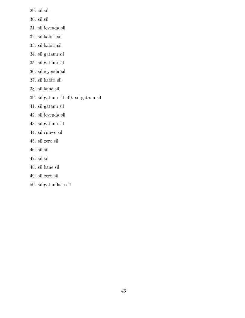
3.2.2 HMM Definition.

The first step in HMM training is to define a prototype model. The purpose of the prototype

is to define a model topology on which all the other models can be based. In HTK a HMM

is a description file and in this case it is

~o

<VecSize>39

<MFCC_0_D_A>

~h "proto"

<BeginHMM>

<NumStates> 6

<State> 2

25

<Mean> 39

0.0 0.0 0.0 0.0 0.0 0.0 0.0 0.0 0.0 0.0 0.0 0.0 0.0

0.0 0.0 0.0 0.0 0.0 0.0 0.0 0.0 0.0 0.0 0.0 0.0 0.0

0.0 0.0 0.0 0.0 0.0 0.0 0.0 0.0 0.0 0.0 0.0 0.0 0.0

<Variance> 39

1.0 1.0 1.0 1.0 1.0 1.0 1.0 1.0 1.0 1.0 1.0 1.0 1.0

1.0 1.0 1.0 1.0 1.0 1.0 1.0 1.0 1.0 1.0 1.0 1.0 1.0

1.0 1.0 1.0 1.0 1.0 1.0 1.0 1.0 1.0 1.0 1.0 1.0 1.0

<State> 3

<Mean> 39

0.0 0.0 0.0 0.0 0.0 0.0 0.0 0.0 0.0 0.0 0.0 0.0 0.0

0.0 0.0 0.0 0.0 0.0 0.0 0.0 0.0 0.0 0.0 0.0 0.0 0.0

0.0 0.0 0.0 0.0 0.0 0.0 0.0 0.0 0.0 0.0 0.0 0.0 0.0

<Variance> 39

1.0 1.0 1.0 1.0 1.0 1.0 1.0 1.0 1.0 1.0 1.0 1.0 1.0

1.0 1.0 1.0 1.0 1.0 1.0 1.0 1.0 1.0 1.0 1.0 1.0 1.0

1.0 1.0 1.0 1.0 1.0 1.0 1.0 1.0 1.0 1.0 1.0 1.0 1.0

<State> 4

<Mean> 39

0.0 0.0 0.0 0.0 0.0 0.0 0.0 0.0 0.0 0.0 0.0 0.0 0.0

0.0 0.0 0.0 0.0 0.0 0.0 0.0 0.0 0.0 0.0 0.0 0.0 0.0

0.0 0.0 0.0 0.0 0.0 0.0 0.0 0.0 0.0 0.0 0.0 0.0 0.0

<Variance> 39

1.0 1.0 1.0 1.0 1.0 1.0 1.0 1.0 1.0 1.0 1.0 1.0 1.0

1.0 1.0 1.0 1.0 1.0 1.0 1.0 1.0 1.0 1.0 1.0 1.0 1.0

1.0 1.0 1.0 1.0 1.0 1.0 1.0 1.0 1.0 1.0 1.0 1.0 1.0

<State> 5

<Mean> 39

0.0 0.0 0.0 0.0 0.0 0.0 0.0 0.0 0.0 0.0 0.0 0.0 0.0

0.0 0.0 0.0 0.0 0.0 0.0 0.0 0.0 0.0 0.0 0.0 0.0 0.0

0.0 0.0 0.0 0.0 0.0 0.0 0.0 0.0 0.0 0.0 0.0 0.0 0.0

26

<Variance> 39

1.0 1.0 1.0 1.0 1.0 1.0 1.0 1.0 1.0 1.0 1.0 1.0 1.0

1.0 1.0 1.0 1.0 1.0 1.0 1.0 1.0 1.0 1.0 1.0 1.0 1.0

1.0 1.0 1.0 1.0 1.0 1.0 1.0 1.0 1.0 1.0 1.0 1.0 1.0

<TransP> 6

0.0 0.5 0.5 0.0 0.0 0.0

0.0 0.4 0.3 0.3 0.0 0.0

0.0 0.0 0.4 0.3 0.3 0.0

0.0 0.0 0.0 0.4 0.3 0.3

0.0 0.0 0.0 0.0 0.5 0.5

0.0 0.0 0.0 0.0 0.0 0.0

<EndHMM>

Models for each of the events were also constructed, see appendix E for the details.

3.2.3 HMM Training

The training described in the parameter estimation introduction can be summarized in a

diagram form as below.

Figure 3.7: HMM training process

27

Initialisation

The HTK tool HInit was used to initialize the data as given below

HInit -A -D -T 1 -S train.scp -M model/hmm0 -H hmmfile -l label -L label dir nameofhmm

where:

nameofhmm is the name of the HMM to initialise (here: yes, no, or sil). hmmfile is a

description file containing the prototype of the HMM called nameofhmm (here: hmm rimwe,

hmm kabiri, e.t.c).

trainlist.txt gives the complete list of the .mfcc files forming the training corpus (stored in

directory data/train/mfc).

label dir is the directory where the label files (.lab) corresponding to the training corpus

(here: data/train/lab/).

label indicates which labelled segment must be used within the training corpus (here: rimwe,

kabiri, etc..

model/hmm0 is the name of the directory (must be created before) where the resulting

initialised HMM description will be output.

This procedure has to be repeated for each model (hmm rimwe, hmm kabiri, hmm gatatu

etc..). The HMM file output by HInit has the same name as the input prototype. E.g

HInit -A -D -T 1 -S train.scp -M model/hmm0 -H hmm 1.txt -l rimwe -L data/train rimwe

This process was repeated for all the models. The HTK tool HCompV was used to initialize

the models to the training data as follows.

HCompV -C config.txt -f 0.01 -m -S train.scp -M hmm0 proto.txt HCompv was not used to

initialise the models (it was already done with HInit). HCompv is only used here because it

outputs, along with the initialised model, an interesting file called vFloors, which contains

the global variance vector multiplied by a factor 0.01 (see Appendix F). The values stored in

varFloor1 (called the ”variance floor macro”) are to be used later during the training process

as floor values for the estimated variance vectors. This results in the creation of two files -

proto and vFloors - in the directory hmm0. These files were edited in the following way: An

error occurs at this point which rearranges the order of the parts of the MFCC 0 D A label

as MFCC D A 0. This was corrected. The first three lines of proto were cut and pasted into

vFloors, this was then saved as macros.

28

3.2.4 Training

The following command line was used to perform one re-estimation iteration with HTK

tool HRest, estimating the optimal values for the HMM parameters (transition probabili-

ties, plus mean and variance vectors of each observation function): HRest -A - D -T 1 -S

train.scp -M model/hmm1 -H vFloors -H model/hmm0/hmm 1.txt -l rimwe -L data/train

rimwe. train.scp gives the complete list of the .mfc files forming the training corpus (stored

in directory data/train/mfc). Model/hmm1, the output directory, indicates the index of

the current iteration. vFloors is the file containing the variance floor macro obtained with

HCompv. Hmm 1.txt is the description file of the HMM called rimwe. It is stored in a

directory whose name indicates the index of the last iteration (here model/hmm0). -l rimwe

is an option that indicates the label to use within the training data (rimwe, kabiri, etc).

Data/train is the directory where the label files (.lab) corresponding to the training corpus.

rimwe is the name of the HMM to train . This procedure has to be repeated several times

for each of the HMMs( kabiri. Gatatu, kane. Sil) to train. Each time, the HRest iterations

(i.e. iterations within the current re-estimation iteration) are displayed on screen, indicating

the convergence through the change measure. As soon as this measure do not decrease (in

absolute value) from one HRest iteration to another, it’s time to stop the process. In this

project 3 re-estimation iterations were used. The final word HMMs are then: hmm3/hmm 1,

hmm3/hmm 0, and hmm3/hmm sil etc.. A file called hmmdefs.txt was created by combin-

ing all the hmms into one file which was consequently named hmmdefs.txt (See appendix E).

After each iteration an error occurred which rearranges the order of the parts of the MFCC 0 D A

label as MFCC D A 0 which was consequently corrected after each iteration.

3.3 Recognition

The recognizer is now complete and its performance can be evaluated. The recognition net-

work and dictionary have already been constructed, and test data has been recorded. Thus,

all that is necessary is to run the recognizer. The recognition process can be summarized as

in the figure below.

29

Figure 3.8: Speech recognition process

An input speech signal input signal is first transformed into a series of ”acoustical vectors”

(here MFCs) using the HTK tool HCopy, in the same way as what was done with the

training data . The result was stored in a file known as test.scp (often called the acoustical

observation).

The input observation was then processed by a Viterbi algorithm, which matches it against

the recogniser’s Markov models using the HTK tool HVite: As follows

HVite -A -D -T 1 -H model/hmm3/hmmdefs.txt -i recout.mlf -w wdnet dict hmmlist.txt -S

test.scp.

Where:

hmmdefs.txt contains the definition of the HMMs. It is possible to repeat the -H option

and list the different HMM definition files, in this case: -H model/hmm3/hmm 0.txt -H

model/hmm3/hmm 1.txt etc.. but it is more convenient (especially when there are more

than 3 models) to gather every definitions in a single file called a Master Macro File. For

this project this file was obtained by copying each definition after the other in a single file,

without repeating the header information (see Appendix E).

The output is stored in a file (recout.mlf) which contains the transcription of the input (see

appendix g).

recout.mlf is the output recognition transcription file.

Wdnet is the task network.

30

dict is the task dictionary.

hmmlist.txt lists the names of the models to use (rimwe, kabiri, etc..). Each element is

separated by a new line character.

Test.scp is the input data to be recognised.

3.4 Running the Recognizer Live

The built recogniser was tested with live input. To do this the configuration variables

parameters were altered as given below # Waveform capture

SOURCERATE=625.0

SOURCEKIND=HAUDIO

SOURCEFORMAT=HTK

ENORMALISE=F

USESILDET=T

MEASURESIL=F

OUTSILWARN=T

These indicate that the source is direct audio with sample period 62.5 secs. The silence

detector is enabled and a measurement of the background speech/silence levels was made at

start-up.The final line makes sure that a warning is printed when this silence measurement

is being made. Once the configuration file had been set-up for direct audio input, the HTK

tool HVite was again used to recognize the live in put using a microphone.

31

Chapter 4

RESULTS

The recognition performance evaluation of an ASR system must be measured on a corpus

of data different from the training corpus. A separate test corpus, with new Kinyarwanda

language digits records, was created as it was previously done with the training corpus. The

test corpus was made of 50 recorded and labelled data which were later converted into MFC.

In order to test for speaker independency of the system, some of the sujects who participated

in creation of the testing corpus had not participated in creation of the training corpus.

4.1 Perfomance Test

Evaluation of the performance of the speech recognition system was done by using the HTK

tool HResults.

On running and testing the tool against the testing data, the following performance statistics

were obtained:

4.2 Perfomance Analysis

The first line (SENT) gives the sentence recognition rate (%Correct=92.00), the second one

(WORD) gives the word recognition rate (%Corr=94.87.00). The first line (SENT) should

32

Figure 4.1: Speech recognition results

be considered here. H=46 gives the number of test data correctly recognized, S=4 the

number of substitution errors and N=50 the total number of test data. These results imply

that of the 50 sentences making the testing corpus only 46 were correctly recognized which

is equivalent to 92.00% and four (4) sentences were substituted by other sentences. The

statistics given on the second line (WORD) only make sense with more sophisticated types

of recognition systems (e.g. connected words recognition tasks). Nevertheless,there were 6

deletion errors (D), 2 substitution errors (S) and 0 insertion errors (I). N 156 gives the total

number of words making the test data and of these 148 were correctly recognized leading to

a 94.87% recognition. The accuracy figure (Acc) of 94.87% is the same as the percentage

correct (Cor) because it takes account of the insertion errors, which the latter does not but

in this case the insertion errors are zero. These results indicate that the training of the

system was successful and and that the developed system is speaker independent.

4.3 Testing the System on Live Data

To further test the system on live data and also again test its speaker independency, the

system was tested by running it live. Four (4) different speakers who never participated in

the creation of the training corpus helped in testing the system live. Subjects read loudly the

Kinyarwanda language numeric digits and the table below gives a summary of the results.

These results show that the system is speaker independent with a few errors which can be

reduced by training the system on a larger training data and also including recordings from

speakers from different regions of the great lakes region who speak Kinyarwanda.

33

Figure 4.2: Live data recognition results

34

Chapter 5

DISCUSSION, CONCLUSION ANDRECOMMENDATIONS

In this project, the main task was to develop an automatic speech recognizer for Kinyarwanda

language. This system is aimed at improving on the current Human-computer interface by

introducing a voice interface, which has proved to have so many advantages to the traditional

I/O methods. Users naturally know how to speak so this would provide an easy interface

which does not necessarily require special training which is normally the case when you’re to

the use the various ICT tools for the first time. The scope was limited to only the numeric

digits which could be used in many systems most especially the automatic telephone dialing

system.

This five chapter report contains the introduction to the study in chapter one and literature

review on human-computer interfaces, ASR and on going African ASR projects. Chapter

three the methodology that was used to achieve the objectives was looked at while chapter

four concentrated on performance and testing the recognizer developed. This is the last

chapter of the report in which the discussion, conclusion and recommendations are given.

5.1 Discussion

It has been discovered that there are many people who have a computer phobia. The reasons

why many people fear to use ICT tools has been due to the indaquate user interfaces which

make it difficult for the new users to explore or take a step into using these unavoidable ICT

tools. A lot has been done by many researchers on improving the user interfaces and one of

35

the improvements has been including voice interfaces. It was noted by the researcher that

most of these systems developed were mainly considering the five major languages Interna-

tional languages.

The researcher therefore, found it necessary to build an ASR system which could be a start-

ing point for many educational and commercial projects on building speech recognisers for

Kinyarwanda language. In order to develop the system, the researcher first read and analysed

research papers on the trends in speech recognition. Then he read reviews on the current

state of the art speech recognisers.

Before attempting building a speech recogniser for a new language it is always advisable to

start by building one language which is already tested and in this case the researcher first

constructed an English Yes and No recogniser which paved the way for the new language

speech recognisers.

The Cambridge University Hidden Markov Models toolkit (HTK) was used for the imple-

mentation of the recogniser. HTK was used because it is free and has been used by many

reaserchers all over the world. HTK supports both isolated whole word recognition and

sub-word or phone based recognition.

Although the research in the area of automatic speech recognition has been pursued for the

last three decades, only whole-word based speech recognition systems have found practical

use and have become commercial successes (Rabiner et al., 1981 [22]; Wilpon et al., 1988

[34]). Two important reasons for this success are that the effects of context-dependence and

co-articulation within the word are implicitly built into the word models and that there is

no necessity of lexical decoding.

Isolated word recognition was considered for this project because it proved to be much easier

because the pauses between the words make it easy to detect the start and end making it

possible to detect each word at a time.

A limited grammar and dictionary were constructed to be used by the recognizer. The

Speech data was recorded and labeled from 6 different speakers making the training and the

testing corpus.

Since the researcher had labeled training data, the HTK tools HInit and HRest were used dur-

ing the initialization and training processing. The results obtained from the system showed

that the system can automatically recognize 94.87 percent words of any Kinyarwanda lan-

36

guage speaker. The system was also tested on live data and it performed well. Four different

speakers participated in the testing of the system on live data and performance was very

good as seen in figure 4.2. There were some cases where the word kane was substituted with

the word karindwi. This problem was mainly observed with some specific speakers not all.

5.2 Conclusion

The objective of this study was mainly to build a speech recognizer for Kinyarwanda language

. In order to meet this objective a limited word grammar was constructed, a dictionary

created and data from different Kinyarwanda language speakers was recorded and trained

thereafter.

The system was tested using testing corpus data and live data and the system scored 92.00%

sentence recognition and 94.87% word recognition. This implies that the objective of creating

a system that can recognize spoken Kinyarwanda language was achieved.

The Kinyarwanda language automatic speech recognition recipe accompanying this report

can be used by any researcher desiring to join language processing research.

The project is however not all conclusive as it has catered for only a voice operated phone

dialing system. As much as it has created a basis for research, this project can be expanded

to cater for more extensive language models and larger vocabularies.

5.3 Areas for Further Study

In spite of the successes of the whole word model speech recognizers which is also exemplified

in the success of this project, they suffer from two problems:

• Co-articulation effects across the word boundaries. This problem has been reasonably

well solved and connected word recognition systems with good performance have been

reported in the literature (Rabiner et al., 1981 [22]; Wilpon et al., 1988 [34]).

• Amount of training data. It is extremely difficult to obtain good whole word reference

models from a limited amount of speech data available for training. This training

problem becomes even worse for large vocabulary speech recognition systems.

37

It is because of the above reasons that I therefore recommend for future research to be taken

in large vocabulary Kinyarwanda language speech recognition, using sub-words (phonemes)

which solve the above mentioned problems. A sub-word based approach is a viable alternative

to the whole-word based approach because here, the word models are built from a small

inventory of sub-word units.

Phoneme HMMs are generalisable (trainable) both towards larger vocabulary and towards

different speakers.

38

REFERENCES

1. Baum, L.E., and Petrie, T., (1966). Statistical Inference for Probabilistic functions of

Finite-State Markov Chains, Annotated Mathematical Statistics,37:1554-1563.

2. Bridle, J., Deng, L., Picone, J., Richards, H., Ma, J., Kamm, T., Schuster, M., Pike,

S., Reagan, R., 1998. An investigation of segmental hidden dynamic models of speech

coarticulation for automatic speech recognition. Final Report for the 1998 Workshop

on Language Engineering, Center for Language and Speech Processing at Johns Hop-

kins University, pp. 161.

3. Cole, R. Noel, M. Burnet, D.C., Fanty,M., Lander, T., Oshika, B., Sutton ,S., 1994

Corpus development activities at the center for spoken language understanding. Hu-

man Language Technology Conference archive, Proceedings of the workshop on Human

Language Technology. Pages: 31 - 36 .

4. R. Cole, K. Roginski, and M. Fanty.,1992 A telephone speech database of spelled and

spoken names. In ICSLP’92, volume 2, pages 891–895.

5. Deshmukh, N., Ganapathiraju, A, Picone J., (1999), Hierarchical Search for Large

Vocabulary Conversational Speech Recognition. IEEE Signal Processing Magazine,

1(5):84-107.

6. Dix, A.J., Finlay,J., Abowd, G., Beale, R. (1998). Human-Computer Interaction, 2nd

edition, Prentice Hall, Englewood Cliffs, NJ,USA.

7. Dupont,S., (2000), Audio-Visual Speech Modeling for Continuous Speech Recognition,

IEEE Transactions on multimedia, 2(3):141-151

39

8. Earth trends, (2003) Population, Health, and Human Well-Being- Rwanda. Retrieved

20-01-2005 from

http://earthtrends.wri.org/pdf library/country profiles/Pop cou 646.pdf.

9. Huang, C., Tao, C., AND Chang,E., (2004). Accent Issues in Large Vocabulary Contin-

uous Speech Recognition INTERNATIONAL JOURNAL OF SPEECH TECHNOLOGY(7):141-

153

10. Jurafsky D., Martin J. (2000). Speech and Language Processing: An Introduction

to Natural Language Processing, Computational Linguistics and Speech Recognition.

Delhi, India: Pearson Education.

11. Kagaba,S., Nsanzabaganwa, S., Mpyisi,E., (2003), Rwanda Country Position Paper,

Regional Workshop on Ageing and Poverty Dar es Salaam, Tanzania.retrieved 20-02-

2005 from

http://www.un.org/esa/socdev/ageing/workshops/tz/rwanda.pdf.

12. Kandasamy, S., (1995),Speech recognition systems. SURPRISE Journal,1(1).

13. Liu, F.H., Liang G., Yuqing G. AND Picheny, M, (2004). Applications of Lan-

guage Modeling in Speech-To-Speech Translation INTERNATIONAL JOURNAL OF

SPEECH TECHNOLOGY (7):221-229.

14. Ma, J., Deng, L., 2004. Target-directed mixture linear dynamic models for spontaneous

speech recognition. IEEE TRANSACTIONS ON SPEECH AND AUDIO PROCESS-

ING, VOL. 12, NO. 1, JANUARY 2004.

15. Ma, J., Deng, L.,2004 A mixed-level switching dynamic system for continuous speech

recognition. Elsevier Computer Speech and Language 18 (2004) 4965.

16. Mane, A., Boyce,S., Karis,D.,Yankelovich,N., (1996) Designing the User Interface for

Speech Recognition Applications SIGCHI Bulletin 28(4):29-34.

17. Mengjie, Z., (2001) Overview of speech recognition and related machine learning tech-

niques, Technical report. retrieved December 10, 2004 from

http://www.mcs.vuw.ac.nz/comp/Publications/archive/CS-TR-01/CS-TR-01-15.pdf

40

18. Mori R.D, Lam L., and Gilloux M. (1987). Learning and plan refinement in a knowledge-

based system for automatic speech recognition. IEEE Transaction on Pattern Analysis

Machine Intelligence, 9(2):289-305.

19. Picheny, M., (2002). Large vocabulary speech recognition, IEEE Computer, 35(4):42-

50.

20. Pinker, S., (1994), The Language Instinct, Harper Collins, New York City, New York,

USA.

21. Rabiner L.R., S.E.L.evinson: (1981) ”Isolated and connected word recognition - Theory

and selected applications”, IEEE Trans. COM-29, pp.621-629

22. Rabiner, L., R., and Wilpon, J. G., (1979). Considerations in applying clustering

techniques to speaker-independent word recognition.Journal of Acoustic Society of

America.66(3):663-673.

23. Reddy D.R., (1976). Speech Recognition by Machine: a Review. Proceeding of IEEE,

64(4):501-531

24. Robertson, J., Wong, Y.T., Chung, C., and Kim, D.K., (1998) Automatic Speech

Recognition for Generalised Time Based Media Retrieval and Indexing, Proceedings of

the sixth ACM International Conference on Multimedia(pp 241-246) Bristol, England.

25. Roux, J.C., Botha, E.C., and Du Preez, J.A., (2000). Developing a Multilingual

Telephone Based Information System in African Languages. Proceedings of the Second

International Language Resources and Evaluation Conference. Athens, Greece:ELRA.

(2):975-980.

26. Rudnicky, A.I., Lee, K.F., and Hauptmann, A.G. (1992) Survey of current speech

technology. Communications of the ACM,37(3):52-57.

27. Scan soft (2004). Embeded speech soloutions retrieved January 25, 2005 from

http://www.speechworks.com/

28. Silverman, H.,F., and Morgan, D.P., (1990). The application of dynamic programming

to connected speech recognition. IEEE ASSP Magazine,7(3):6-25.

41

29. Svendsen T., Paliwal K. K., Harborg E., Husy P. O. (1989). Proc. ICASSP’89, Glas-

gow,

30. Tiong, B., (1997) Speech Recognition retrieved December 10, 2004 from

http://murray.newcastle.edu.au/users/staff/speech/home pages/tutorial sr.html.

31. Tolba, H., and O’Shaughnessy, D., (2001). Speech Recognition by Intelligent Machines,

IEEE Canadian Review (38).

32. Warwick, C., 1997 What is the BNC? [Online]. Available from World Wide Web:

http://www.hcu.ox.ac.uk/BNC¿ retrieved on 20-05-2005.

33. Webster’s dictionary (2004). illiterate retrieved September 23, 2004 from http://www.webster-

dictionary.org/definition/illiterate.

34. Wilpon J.G., D.M.DeMarco,R.P.Mikkilineni (1988) ”Isolated word recognition over

the DD telephone network -Results of two extensive field studies”, Proc. ICASSP,pp.

55-58

35. Young, S., G. Evermann, T. Hain, D. Kershaw, G. Moore, J. Odell, D. Ollason, D.

Povey, V. Valtchev, P. Woodland,( 2002) The HTK Book. Retrieved April 1, 2005

from: http://htk.eng.cam.ac.uk.

36. Zue, V., Cole, R., Ward, W. (1996). Speech Recognition.Survey of the State of the Art

in Human Language Technology. Kauii, Hawaii, USA

42

APPENDICES

Apendix A

Word Network

VERSION=1.0

N=15 L=24

I=0 W=!NULL

I=1 W=!NULL

I=2 W=SENT-START

I=3 W=RIMWE

I=4 W=!NULL

I=5 W=KABIRI

I=6 W=GATATU

I=7 W=KANE

I=8 W=GATANU

I=9 W=GATANDATU

I=10 W=KARINDWI

I=11 W=UMUNANI

I=12 W=ICYENDA

I=13 W=ZERO

I=14 W=SENT-END

J=0 S=14 E=1

J=1 S=0 E=2

J=2 S=2 E=3

43

J=3 S=3 E=4

J=4 S=5 E=4

J=5 S=6 E=4

J=6 S=7 E=4

J=7 S=8 E=4

J=8 S=9 E=4

J=9 S=10 E=4

J=10 S=11 E=4

J=11 S=12 E=4

J=12 S=13 E=4

J=13 S=2 E=5

J=14 S=2 E=6

J=15 S=2 E=7

J=16 S=2 E=8

J=17 S=2 E=9

J=18 S=2 E=10

J=19 S=2 E=11

J=20 S=2 E=12

J=21 S=2 E=13

J=22 S=2 E=14

J=23 S=4 E=14

44

Appendix B

Training Sentences

1. sil sil

2. sil gatatu sil

3. sil gatanu sil

4. sil gatanu sil

5. sil sil

6. sil karindwi sil

7. sil zero sil

8. sil umunani sil

9. sil gatanu sil

10. sil kane sil

11. sil icyenda sil

12. sil zero sil

13. sil icyenda sil

14. sil gatandatu sil

15. sil zero sil

16. sil sil

17. sil umunani sil

18. sil umunani sil

19. sil gatatu sil


21. sil karindwi sil

22. sil kane sil

23. sil karindwi sil


25. sil kane sil

26. sil gatanu sil

27. sil gatatu sil

28. sil zero sil

45

29. sil sil

30. sil sil

31. sil icyenda sil

32. sil kabiri sil

33. sil kabiri sil

34. sil gatanu sil

35. sil gatanu sil

36. sil icyenda sil

37. sil kabiri sil

38. sil kane sil

39. sil gatanu sil 40. sil gatanu sil

41. sil gatanu sil

42. sil icyenda sil

43. sil gatanu sil

44. sil rimwe sil

45. sil zero sil

46. sil sil

47. sil sil

48. sil kane sil

49. sil zero sil


46

Appendix C

Master label file

#!MLF!#


RIMWE

.


RIMWE

.


RIMWE

.


RIMWE

.


RIMWE

.


RIMWE

.


RIMWE

.


RIMWE

.


RIMWE

.

47


RIMWE

.

”data/train/rimwe11.lab” RIMWE

.


.


.


.


.

”data/train/kabiri01.lab”

KABIRI

.


KABIRI

.


KABIRI

.


KABIRI

.


KABIRI

.


KABIRI

.

48


KABIRI

.


KABIRI

.


KABIRI

.


KABIRI

.


KABIRI

.


KABIRI

.


KABIRI

.


KABIRI

.


KABIRI

.


KABIRI

.


49

KABIRI

.

”data/train/gatatu01.lab”

GATATU

.


GATATU

.


GATATU

.


GATATU

.


GATATU

.


GATATU

.


GATATU

.


GATATU

.


GATATU

.


GATATU

50

.


GATATU

.


GATATU

.


GATATU

.


GATATU

.


GATATU

.

”data/train/kane01.lab”

KANE

.


KANE

.


KANE

.


KANE

.


KANE

.

51


KANE

.


KANE

.


KANE

.


KANE

.


KANE

.


KANE

.


KANE

.


KANE

.


KANE

.


KANE

.

”data/train/gatanu01.lab”

52

GATANU

.


GATANU

.


GATANU

.


GATANU

.


GATANU

.


GATANU

.


GATANU

.


GATANU

.


GATANU

.


GATANU

.


GATANU

53

.


GATANU

.


GATANU

.


GATANU

.


GATANU

.

”data/train/gatandatu01.lab”

GATANDATU

.


GATANDATU

.


GATANDATU

.


GATANDATU

.


GATANDATU

.


GATANDATU

.

54


GATANDATU

.


GATANDATU

.


GATANDATU

.


GATANDATU

.


GATANDATU

.


GATANDATU

.


GATANDATU

.


GATANDATU

.


GATANDATU

.

”data/train/karindwi01.lab”

KARINDWI

.


55

KARINDWI

.


KARINDWI

.


KARINDWI

.


KARINDWI

.


KARINDWI

.


KARINDWI .


KARINDWI

.


KARINDWI

.


KARINDWI

.


KARINDWI

.


KARINDWI

.

56


KARINDWI

.


KARINDWI

.


KARINDWI

.

”data/train/umunani01.lab”

UMUNANI

.


UMUNANI

.


UMUNANI

.


UMUNANI

.


UMUNANI

.


UMUNANI

.


UMUNANI

.


57

UMUNANI

.


UMUNANI

.


UMUNANI

.


UMUNANI

.


UMUNANI

.


UMUNANI

.


UMUNANI

.


UMUNANI

.

”data/train/icyenda01.lab”

ICYENDA

.


ICYENDA

.


ICYENDA

58

.


ICYENDA

.


ICYENDA

.


ICYENDA

.


ICYENDA

.


ICYENDA

.


ICYENDA

.


ICYENDA

.


ICYENDA

.


ICYENDA

.


ICYENDA

.

59


ICYENDA

.


ICYENDA

.

”data/train/zero01.lab”

ZERO

.


ZERO

.


ZERO

.


ZERO

.


ZERO

.


ZERO

.


ZERO

.


ZERO

.

60


ZERO

.


ZERO

.


ZERO

.


ZERO

.


ZERO

.


ZERO

.


ZERO

61

Appendix D

Training Data

data/MFC/rimwe01.MFC















data/MFC/kabiri01.MFC













62



data/MFC/gatatu01.MFC















data/MFC/kane01.MFC

data/MFC/kane02.MFC

data/MFC/kane03.MFC

data/MFC/kane04.MFC

data/MFC/kane05.MFC

data/MFC/kane06.MFC

data/MFC/kane07.MFC

data/MFC/kane08.MFC

data/MFC/kane09.MFC

data/MFC/kane10.MFC

data/MFC/kane11.MFC

data/MFC/kane12.MFC

data/MFC/kane13.MFC

data/MFC/kane14.MFC

63

data/MFC/kane15.MFC

data/MFC/gatanu01.MFC















data/MFC/gatandatu01.MFC















64

data/MFC/karindwi01.MFC















data/MFC/umunani01.MFC















data/MFC/icyenda01.MFC

65















data/MFC/zero01.MFC

data/MFC/zero02.MFC

data/MFC/zero03.MFC

data/MFC/zero04.MFC

data/MFC/zero05.MFC

data/MFC/zero06.MFC

data/MFC/zero07.MFC

data/MFC/zero08.MFC

data/MFC/zero09.MFC

data/MFC/zero10.MFC

data/MFC/zero11.MFC

data/MFC/zero12.MFC

data/MFC/zero13.MFC

data/MFC/zero14.MFC

data/MFC/zero15.MFC

66

Appendix E

Hidden Markov Model Definitions (HMMDEFS)

~o

<STREAMINFO> 1 39

<VECSIZE> 39<NULLD><MFCC_0_D_A><DIAGC>

~h "zero"

<BEGINHMM>

<NUMSTATES> 6

<STATE> 2

<MEAN> 39

-1.538187e+001 1.141508e+001 -3.588139e+000 -1.159882e+000 -1.452020e+000 -8.341283e+000

<VARIANCE> 39

3.046115e+001 3.921619e+001 1.723766e+001 2.001421e+001 3.992482e+001 3.596347e+001 2.784846e+001

<GCONST> 1.137821e+002

<STATE> 3

<MEAN> 39

-1.491195e+000 -6.492606e+000 -1.891563e-001 -6.878118e+000 -6.327397e+000 -1.235269e+001

<VARIANCE> 39

2.520783e+000 8.964164e+000 5.252084e+000 8.973154e+000 5.499793e+000 1.332134e+001 2.178135e+001

<GCONST> 9.035600e+001

<STATE> 4

<MEAN> 39

-9.309770e+000 -9.457813e+000 -2.599780e+000 -1.757934e+001 -1.275383e+001 -1.126780e+001

<VARIANCE> 39

6.970012e+001 2.225276e+001 4.992588e+001 4.126175e+001 2.610523e+001 7.679757e+001 6.116331e+001

<GCONST> 1.238130e+002

<STATE> 5

<MEAN> 39

-2.297705e-001 -4.164129e-002 -1.899639e+000 -9.609221e+000 -5.382258e+000 -1.236597e+000

67

<VARIANCE> 39

8.854380e+000 7.536385e+000 1.740920e+001 4.921722e+001 3.659902e+001 1.955439e+001 4.722785e+001

<GCONST> 1.009971e+002

<TRANSP> 6

0.000000e+000 1.000000e+000 0.000000e+000 0.000000e+000 0.000000e+000 0.000000e+000

0.000000e+000 9.060647e-001 6.262358e-002 3.131179e-002 0.000000e+000 0.000000e+000

0.000000e+000 0.000000e+000 9.430364e-001 5.696366e-002 0.000000e+000 0.000000e+000

0.000000e+000 0.000000e+000 0.000000e+000 9.249576e-001 7.504237e-002 0.000000e+000

0.000000e+000 0.000000e+000 0.000000e+000 0.000000e+000 8.498170e-001 1.501830e-001

0.000000e+000 0.000000e+000 0.000000e+000 0.000000e+000 0.000000e+000 0.000000e+000

<ENDHMM>

~h "rimwe"

<BEGINHMM>

<NUMSTATES> 6

<STATE> 2

<MEAN> 39

-7.970719e+000 -7.500427e+000 1.132444e+001 -1.286703e+001 -7.432399e+000 -1.751952e+001

<VARIANCE> 39

3.849774e+001 2.229306e+001 4.268061e+001 8.451440e+001 3.439103e+001 4.802508e+001 5.185015e+001

<GCONST> 1.317715e+002

<STATE> 3

<MEAN> 39

-2.377380e+000 -3.663290e+000 4.965676e+000 -1.033556e+001 -7.324887e+000 -1.087329e+001

<VARIANCE> 39

7.865341e+000 1.011867e+001 4.059527e+000 3.692888e+001 2.392439e+001 1.843463e+001 3.225859e+001

<GCONST> 1.058150e+002

<STATE> 4

<MEAN> 39

-7.165953e+000 -6.947466e+000 6.544258e+000 -1.652563e+001 -9.213765e+000 -1.855777e+001

<VARIANCE> 39

3.759945e+001 6.370345e+000 9.036909e+000 1.956501e+002 2.907838e+001 4.600018e+001 2.415433e+001

68

<GCONST> 1.079340e+002

<STATE> 5

<MEAN> 39

-6.314114e+000 -4.532432e+000 7.106805e+000 -7.048369e+000 -8.000018e+000 -1.071996e+001

<VARIANCE> 39

2.019156e+001 3.633694e+001 1.606951e+001 1.441847e+002 5.447787e+001 4.976671e+001 2.165058e+001

<GCONST> 1.010713e+002

<TRANSP> 6

0.000000e+000 9.333376e-001 6.666239e-002 0.000000e+000 0.000000e+000 0.000000e+000

0.000000e+000 9.137994e-001 8.620062e-002 0.000000e+000 0.000000e+000 0.000000e+000

0.000000e+000 0.000000e+000 8.917421e-001 1.082579e-001 0.000000e+000 0.000000e+000

0.000000e+000 0.000000e+000 0.000000e+000 8.244619e-001 1.755382e-001 0.000000e+000

0.000000e+000 0.000000e+000 0.000000e+000 0.000000e+000 9.221094e-001 7.789055e-002

0.000000e+000 0.000000e+000 0.000000e+000 0.000000e+000 0.000000e+000 0.000000e+000

<ENDHMM>

~h "kabiri"

<BEGINHMM>

<NUMSTATES> 6

<STATE> 2

<MEAN> 39

-7.888013e+000 -1.187933e+001 -2.681767e+000 -1.294684e+001 1.227886e+000 -9.493131e+000

<VARIANCE> 39

4.862306e+001 1.635481e+001 3.838939e+001 3.666690e+001 4.893019e+001 3.454409e+001 4.188983e+001

<GCONST> 1.329512e+002

<STATE> 3

<MEAN> 39

-1.659296e+000 -7.659583e+000 8.000670e+000 -1.012939e+000 -4.288243e+000 -1.464354e+001

<VARIANCE> 39

8.231427e+000 6.313235e+000 6.235238e+001 3.491607e+001 1.448567e+001 1.007993e+001 1.463966e+001

<GCONST> 9.725203e+001

<STATE> 4

69

<MEAN> 39

-7.019081e+000 -4.749569e+000 1.820031e+001 -9.001300e+000 -8.113852e+000 -1.175638e+001

<VARIANCE> 39

9.790601e+000 2.004658e+001 1.836600e+001 3.005601e+001 2.896993e+001 3.778489e+001 1.294033e+001

<GCONST> 1.157377e+002

<STATE> 5

<MEAN> 39

-1.058715e+001 -7.019902e-001 1.127821e+001 -2.145595e+001 -6.475991e+000 -1.326184e+001

<VARIANCE> 39

4.183236e+001 3.304543e+001 2.711980e+001 1.644754e+002 4.248949e+001 5.100737e+001 2.856202e+001

<GCONST> 1.120947e+002

<TRANSP> 6

0.000000e+000 1.000000e+000 0.000000e+000 0.000000e+000 0.000000e+000 0.000000e+000

0.000000e+000 9.191111e-001 8.088891e-002 0.000000e+000 0.000000e+000 0.000000e+000

0.000000e+000 0.000000e+000 8.458276e-001 1.130628e-001 4.110956e-002 0.000000e+000

0.000000e+000 0.000000e+000 0.000000e+000 9.421099e-001 5.789007e-002 0.000000e+000

0.000000e+000 0.000000e+000 0.000000e+000 0.000000e+000 9.339923e-001 6.600768e-002

0.000000e+000 0.000000e+000 0.000000e+000 0.000000e+000 0.000000e+000 0.000000e+000

<ENDHMM>

~o

<STREAMINFO> 1 39

<VECSIZE> 39<NULLD><MFCC_0_D_A><DIAGC>

~h "kabiri"

<BEGINHMM>

<NUMSTATES> 6

<STATE> 2

<MEAN> 39

-7.888013e+000 -1.187933e+001 -2.681767e+000 -1.294684e+001 1.227886e+000 -9.493131e+000

<VARIANCE> 39

4.862306e+001 1.635481e+001 3.838939e+001 3.666690e+001 4.893019e+001 3.454409e+001 4.188983e+001

<GCONST> 1.329512e+002

70

<STATE> 3

<MEAN> 39

-1.659296e+000 -7.659583e+000 8.000670e+000 -1.012939e+000 -4.288243e+000 -1.464354e+001

<VARIANCE> 39

8.231427e+000 6.313235e+000 6.235238e+001 3.491607e+001 1.448567e+001 1.007993e+001 1.463966e+001

<GCONST> 9.725203e+001

<STATE> 4

<MEAN> 39

-7.019081e+000 -4.749569e+000 1.820031e+001 -9.001300e+000 -8.113852e+000 -1.175638e+001

<VARIANCE> 39

9.790601e+000 2.004658e+001 1.836600e+001 3.005601e+001 2.896993e+001 3.778489e+001 1.294033e+001

<GCONST> 1.157377e+002

<STATE> 5

<MEAN> 39

-1.058715e+001 -7.019902e-001 1.127821e+001 -2.145595e+001 -6.475991e+000 -1.326184e+001

<VARIANCE> 39

4.183236e+001 3.304543e+001 2.711980e+001 1.644754e+002 4.248949e+001 5.100737e+001 2.856202e+001

<GCONST> 1.120947e+002

<TRANSP> 6

0.000000e+000 1.000000e+000 0.000000e+000 0.000000e+000 0.000000e+000 0.000000e+000

0.000000e+000 9.191111e-001 8.088891e-002 0.000000e+000 0.000000e+000 0.000000e+000

0.000000e+000 0.000000e+000 8.458276e-001 1.130628e-001 4.110956e-002 0.000000e+000

0.000000e+000 0.000000e+000 0.000000e+000 9.421099e-001 5.789007e-002 0.000000e+000

0.000000e+000 0.000000e+000 0.000000e+000 0.000000e+000 9.339923e-001 6.600768e-002

0.000000e+000 0.000000e+000 0.000000e+000 0.000000e+000 0.000000e+000 0.000000e+000

<ENDHMM>

~h "gatatu"

<BEGINHMM>

<NUMSTATES> 6

<STATE> 2

<MEAN> 39

71

-7.390771e+000 -5.917681e+000 -2.103130e+000 -9.950102e+000 -3.979828e+000 -1.047798e+001

<VARIANCE> 39

3.005470e+001 3.006998e+001 2.985134e+001 5.186708e+001 3.257998e+001 5.920473e+001 7.331139e+001

<GCONST> 1.438623e+002

<STATE> 3

<MEAN> 39

-4.205491e+000 -3.322559e+000 -1.800535e+000 -7.406120e+000 -5.095723e+000 -8.503020e+000

<VARIANCE> 39

1.636298e+001 1.398440e+001 5.007754e+000 1.967910e+001 1.182736e+001 9.890709e+000 1.357527e+001

<GCONST> 1.011073e+002

<STATE> 4

<MEAN> 39

-1.168745e+001 -3.924672e+000 1.028068e+000 -9.808208e+000 -4.435424e-002 -5.277567e+000

<VARIANCE> 39

1.160676e+001 2.277476e+001 2.329525e+001 3.608196e+001 3.057339e+001 2.757198e+001 3.247049e+001

<GCONST> 1.214261e+002

<STATE> 5

<MEAN> 39

2.013859e-001 7.833384e-001 -2.304667e+000 -1.186296e+001 -2.866407e+000 -4.851678e+000

<VARIANCE> 39

1.207510e+001 8.797694e+000 1.094520e+001 3.902149e+001 1.363658e+001 2.133236e+001 3.828735e+001

<GCONST> 1.057806e+002

<TRANSP> 6

0.000000e+000 1.000000e+000 0.000000e+000 0.000000e+000 0.000000e+000 0.000000e+000

0.000000e+000 9.553569e-001 3.017069e-002 1.447246e-002 0.000000e+000 0.000000e+000

0.000000e+000 0.000000e+000 9.361491e-001 6.385095e-002 0.000000e+000 0.000000e+000

0.000000e+000 0.000000e+000 0.000000e+000 9.064240e-001 9.357602e-002 0.000000e+000

0.000000e+000 0.000000e+000 0.000000e+000 0.000000e+000 9.347656e-001 6.523441e-002

0.000000e+000 0.000000e+000 0.000000e+000 0.000000e+000 0.000000e+000 0.000000e+000

<ENDHMM>

~h "kane"

72

<BEGINHMM>

<NUMSTATES> 6

<STATE> 2

<MEAN> 39

-8.057542e+000 -1.060878e+001 -4.268703e+000 -1.086176e+001 8.497649e-002 -5.583869e+000

<VARIANCE> 39

4.903220e+001 1.778465e+001 2.172715e+001 3.269134e+001 5.859225e+001 2.064451e+001 4.554149e+001

<GCONST> 1.328887e+002

<STATE> 3

<MEAN> 39

-7.654702e+000 -5.980002e+000 6.218244e+000 -1.785333e+001 -1.128413e+001 -1.349626e+001

<VARIANCE> 39

3.431395e+001 3.294825e+001 7.759271e+000 5.328711e+001 1.814535e+001 2.150519e+001 2.093969e+001

<GCONST> 1.236389e+002

<STATE> 4

<MEAN> 39

-2.756640e+000 -8.790867e+000 7.811357e+000 -1.539050e+001 -1.123307e+001 -1.232298e+001

<VARIANCE> 39

5.670832e-001 2.651911e+000 2.599197e+000 3.942507e+000 5.074362e+000 4.935444e+000 9.304113e+000

<GCONST> 6.399265e+001

<STATE> 5

<MEAN> 39

-6.698071e+000 -1.129157e+000 8.156453e+000 -1.402400e+001 -7.723018e+000 -5.042853e+000

<VARIANCE> 39

2.265060e+001 1.672502e+001 2.089884e+001 7.828613e+001 3.141041e+001 3.859872e+001 1.680197e+001

<GCONST> 1.026692e+002

<TRANSP> 6

0.000000e+000 1.000000e+000 0.000000e+000 0.000000e+000 0.000000e+000 0.000000e+000

0.000000e+000 9.240341e-001 7.596595e-002 0.000000e+000 0.000000e+000 0.000000e+000

0.000000e+000 0.000000e+000 8.692063e-001 8.719578e-002 4.359789e-002 0.000000e+000

0.000000e+000 0.000000e+000 0.000000e+000 9.010528e-001 9.894721e-002 0.000000e+000

73

0.000000e+000 0.000000e+000 0.000000e+000 0.000000e+000 8.704605e-001 1.295396e-001

0.000000e+000 0.000000e+000 0.000000e+000 0.000000e+000 0.000000e+000 0.000000e+000

<ENDHMM>

~h "gatanu"

<BEGINHMM>

<NUMSTATES> 6

<STATE> 2

<MEAN> 39

-2.673798e+000 -9.356992e+000 5.441325e-001 -1.141471e+001 -1.703487e+000 -1.510815e+001

<VARIANCE> 39

1.248814e+001 1.846922e+001 1.526149e+001 4.118730e+001 2.809689e+001 2.215244e+001 7.992797e+001

<GCONST> 1.285426e+002

<STATE> 3

<MEAN> 39

-9.179394e+000 -4.328063e+000 -6.742033e-001 -7.842070e+000 -3.467945e+000 -6.189126e+000

<VARIANCE> 39

2.638436e+001 2.927450e+001 3.584095e+001 3.864722e+001 2.810151e+001 2.947144e+001 3.752283e+001

<GCONST> 1.320189e+002

<STATE> 4

<MEAN> 39

-6.039360e+000 -1.091987e+001 -5.664576e+000 -1.614972e+001 -1.432853e+000 -4.402873e+000

<VARIANCE> 39

4.627198e+001 1.405917e+001 2.971918e+001 1.565750e+001 3.092512e+001 4.182518e+001 4.819402e+001

<GCONST> 1.119498e+002

<STATE> 5

<MEAN> 39

-2.673770e+000 -1.938864e+000 2.444091e+000 -1.066288e+001 -5.001587e+000 -8.596553e+000

<VARIANCE> 39

1.219363e+001 8.865636e+000 1.369036e+001 1.443630e+001 1.524414e+001 3.601057e+001 2.025958e+001

<GCONST> 9.604260e+001

<TRANSP> 6

74

0.000000e+000 1.000000e+000 0.000000e+000 0.000000e+000 0.000000e+000 0.000000e+000

0.000000e+000 8.672363e-001 1.327637e-001 0.000000e+000 0.000000e+000 0.000000e+000

0.000000e+000 0.000000e+000 9.390594e-001 6.094063e-002 0.000000e+000 0.000000e+000

0.000000e+000 0.000000e+000 0.000000e+000 9.379871e-001 6.201285e-002 0.000000e+000

0.000000e+000 0.000000e+000 0.000000e+000 0.000000e+000 9.489780e-001 5.102201e-002

0.000000e+000 0.000000e+000 0.000000e+000 0.000000e+000 0.000000e+000 0.000000e+000

<ENDHMM>

~h "gatandatu"

<BEGINHMM>

<NUMSTATES> 6

<STATE> 2

<MEAN> 39

-1.015873e+001 -7.870405e+000 -1.680081e+000 -1.051597e+001 -3.550692e+000 -7.160385e+000

<VARIANCE> 39

3.556055e+001 4.019184e+001 3.388691e+001 4.676527e+001 4.065084e+001 7.829738e+001 6.061843e+001

<GCONST> 1.409927e+002

<STATE> 3

<MEAN> 39

-1.339054e+000 -6.674555e+000 1.699593e+000 -1.258614e+001 -3.930208e+000 -9.488519e+000

<VARIANCE> 39

3.638019e+000 1.876286e+001 1.732436e+001 1.563778e+001 1.900627e+001 1.131656e+001 4.601906e+001

<GCONST> 1.138005e+002

<STATE> 4

<MEAN> 39

-9.892857e+000 -1.979889e+000 8.483336e-001 -7.349046e+000 -1.613775e+000 -5.763394e+000

<VARIANCE> 39

8.659358e+000 8.861095e+000 1.427904e+001 1.546748e+001 3.311852e+001 2.053959e+001 4.144904e+001

<GCONST> 1.110476e+002

<STATE> 5

<MEAN> 39

2.401667e-001 -1.656038e+000 4.144118e-001 -8.085937e+000 -1.530486e+000 -4.962093e+000

75

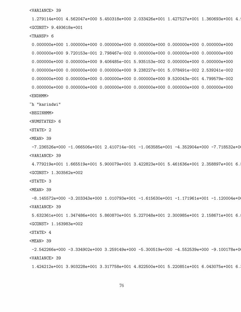
<VARIANCE> 39

1.279114e+001 4.562047e+000 5.450318e+000 2.033426e+001 1.427527e+001 1.360693e+001 4.941040e+001

<GCONST> 9.493618e+001

<TRANSP> 6

0.000000e+000 1.000000e+000 0.000000e+000 0.000000e+000 0.000000e+000 0.000000e+000

0.000000e+000 9.720153e-001 2.798467e-002 0.000000e+000 0.000000e+000 0.000000e+000

0.000000e+000 0.000000e+000 9.406485e-001 5.935153e-002 0.000000e+000 0.000000e+000

0.000000e+000 0.000000e+000 0.000000e+000 9.238227e-001 5.078491e-002 2.539241e-002

0.000000e+000 0.000000e+000 0.000000e+000 0.000000e+000 9.520043e-001 4.799579e-002

0.000000e+000 0.000000e+000 0.000000e+000 0.000000e+000 0.000000e+000 0.000000e+000

<ENDHMM>

~h "karindwi"

<BEGINHMM>

<NUMSTATES> 6

<STATE> 2

<MEAN> 39

-7.236526e+000 -1.066506e+001 2.410714e-001 -1.063585e+001 -4.352904e+000 -7.718532e+000

<VARIANCE> 39

4.779219e+001 1.665519e+001 5.900079e+001 3.422823e+001 5.461636e+001 2.358897e+001 6.535747e+001

<GCONST> 1.303562e+002

<STATE> 3

<MEAN> 39

-8.145572e+000 -3.203343e+000 1.010793e+001 -1.615630e+001 -1.171961e+001 -1.120004e+001

<VARIANCE> 39

5.632361e+001 1.347486e+001 5.860870e+001 5.227048e+001 2.300985e+001 2.158671e+001 6.898752e+001

<GCONST> 1.163983e+002

<STATE> 4

<MEAN> 39

-2.542266e+000 -3.334902e+000 3.259149e+000 -5.300519e+000 -4.552539e+000 -9.100178e+000

<VARIANCE> 39

1.424212e+001 3.903228e+001 3.317758e+001 4.822500e+001 5.220851e+001 6.043075e+001 6.323088e+001

76

<GCONST> 1.407230e+002

<STATE> 5

<MEAN> 39

-7.458948e+000 -3.782425e+000 9.387439e+000 -1.012991e+001 -1.045399e+001 -7.275731e+000

<VARIANCE> 39

2.919024e+001 2.421864e+001 4.132079e+001 7.579975e+001 8.122581e+001 5.412838e+001 6.227592e+001

<GCONST> 1.183515e+002

<TRANSP> 6

0.000000e+000 1.000000e+000 0.000000e+000 0.000000e+000 0.000000e+000 0.000000e+000

0.000000e+000 9.402466e-001 5.975344e-002 0.000000e+000 0.000000e+000 0.000000e+000

0.000000e+000 0.000000e+000 9.431054e-001 5.689462e-002 0.000000e+000 0.000000e+000

0.000000e+000 0.000000e+000 0.000000e+000 9.348174e-001 6.518257e-002 0.000000e+000

0.000000e+000 0.000000e+000 0.000000e+000 0.000000e+000 9.450952e-001 5.490478e-002

0.000000e+000 0.000000e+000 0.000000e+000 0.000000e+000 0.000000e+000 0.000000e+000

<ENDHMM>

~h "umunani"

<BEGINHMM>

<NUMSTATES> 6

<STATE> 2

<MEAN> 39

1.681069e+000 2.597972e-001 -2.102225e+000 -1.272634e+001 -7.886747e+000 -4.786170e+000

<VARIANCE> 39

1.240989e+001 1.048145e+001 2.223962e+001 2.924567e+001 2.658429e+001 2.185395e+001 2.165411e+001

<GCONST> 1.141408e+002

<STATE> 3

<MEAN> 39

-9.025550e+000 -7.838059e+000 1.823010e-001 -1.517856e+001 -7.216865e+000 -1.019580e+001

<VARIANCE> 39

4.965593e+001 4.002261e+001 3.900344e+001 6.009333e+001 4.482301e+001 4.609790e+001 5.317699e+001

<GCONST> 1.324766e+002

<STATE> 4

77

<MEAN> 39

-3.113127e+000 -6.011573e+000 -4.997765e-002 -1.301623e+001 -5.893340e+000 -9.431502e+000

<VARIANCE> 39

1.965076e+000 1.852885e+001 3.407612e+001 1.203665e+001 8.759190e+000 1.875137e+001 3.306817e+001

<GCONST> 1.023604e+002

<STATE> 5

<MEAN> 39

-6.238905e+000 1.952969e+000 8.139153e+000 -1.412227e+001 -5.182961e+000 -4.409090e+000

<VARIANCE> 39

1.011204e+001 5.521096e+000 2.187045e+001 6.730286e+001 2.985188e+001 3.386910e+001 3.464477e+001

<GCONST> 9.443905e+001

<TRANSP> 6

0.000000e+000 1.000000e+000 0.000000e+000 0.000000e+000 0.000000e+000 0.000000e+000

0.000000e+000 9.228172e-001 7.718279e-002 0.000000e+000 0.000000e+000 0.000000e+000

0.000000e+000 0.000000e+000 9.619250e-001 2.538341e-002 1.269155e-002 0.000000e+000

0.000000e+000 0.000000e+000 0.000000e+000 9.631567e-001 3.684329e-002 0.000000e+000

0.000000e+000 0.000000e+000 0.000000e+000 0.000000e+000 9.365148e-001 6.348520e-002

0.000000e+000 0.000000e+000 0.000000e+000 0.000000e+000 0.000000e+000 0.000000e+000

<ENDHMM>

~h "icyenda"

<BEGINHMM>

<NUMSTATES> 6

<STATE> 2

<MEAN> 39

-1.539500e+001 1.913122e+000 4.892755e+000 -7.411077e+000 -3.252254e+000 -4.670670e+000

<VARIANCE> 39

3.937204e+001 2.366165e+001 2.901213e+001 7.555241e+001 3.239333e+001 4.215692e+001 4.146538e+001

<GCONST> 1.331492e+002

<STATE> 3

<MEAN> 39

-9.767091e+000 -7.412555e+000 -7.954957e-001 -1.257044e+001 -9.115961e+000 -1.128199e+001

78

<VARIANCE> 39

6.789838e+001 8.131030e+000 2.133095e+001 1.963373e+001 1.534718e+001 4.011393e+001 4.208259e+001

<GCONST> 1.051703e+002

<STATE> 4

<MEAN> 39

-4.214276e+000 -3.088863e+000 5.680709e+000 -1.330309e+001 -1.153709e+001 -9.793489e+000

<VARIANCE> 39

3.400375e+001 3.902774e+001 1.417232e+001 5.824862e+001 2.261618e+001 3.309546e+001 3.816209e+001

<GCONST> 1.305070e+002

<STATE> 5

<MEAN> 39

-3.845330e+000 -7.520312e+000 -4.539398e+000 -1.070767e+001 -7.937269e-001 -4.884501e+000

<VARIANCE> 39

1.816542e+001 2.136757e+001 1.688432e+001 2.374783e+001 2.672420e+001 2.343285e+001 3.595092e+001

<GCONST> 1.102168e+002

<TRANSP> 6

0.000000e+000 1.000000e+000 0.000000e+000 0.000000e+000 0.000000e+000 0.000000e+000

0.000000e+000 9.504286e-001 4.957141e-002 0.000000e+000 0.000000e+000 0.000000e+000

0.000000e+000 0.000000e+000 9.002472e-001 9.975278e-002 0.000000e+000 0.000000e+000

0.000000e+000 0.000000e+000 0.000000e+000 9.299484e-001 7.005156e-002 0.000000e+000

0.000000e+000 0.000000e+000 0.000000e+000 0.000000e+000 9.361448e-001 6.385522e-002

0.000000e+000 0.000000e+000 0.000000e+000 0.000000e+000 0.000000e+000 0.000000e+000

<ENDHMM>

~h "sil"

<BEGINHMM>

<NUMSTATES> 6

<STATE> 2

<MEAN> 39

-1.166347e+001 -2.349667e+000 6.230773e-001 -5.791427e+000 -3.163599e+000 -3.262644e+000

<VARIANCE> 39

1.801193e+001 1.427911e+001 2.757210e+001 3.023239e+001 2.781987e+001 3.004006e+001 2.759418e+001

79

<GCONST> 1.008924e+002

<STATE> 3

<MEAN> 39

-8.603083e+000 2.727572e+000 3.617722e+000 1.818626e+000 3.906403e-001 3.107029e-001 -6.671149e-001

<VARIANCE> 39

7.133804e+000 6.455761e+000 8.630907e+000 1.268900e+001 1.100004e+001 1.200856e+001 1.464770e+001

<GCONST> 7.239511e+001

<STATE> 4

<MEAN> 39

-1.287919e+001 -1.880384e+000 -2.084125e+000 -2.492788e+000 -3.290475e+000 -3.127917e+000

<VARIANCE> 39

3.802010e+000 4.608351e+000 6.783229e+000 1.065659e+001 1.005600e+001 1.236252e+001 1.405560e+001

<GCONST> 6.763563e+001

<STATE> 5

<MEAN> 39

-1.074988e+001 -1.872770e+000 3.384747e-001 -3.966482e+000 -1.400925e+000 -4.761750e+000

<VARIANCE> 39

1.933378e+001 4.053452e+001 2.861359e+001 4.188812e+001 3.746236e+001 3.709630e+001 5.393936e+001

<GCONST> 1.274157e+002

<TRANSP> 6

0.000000e+000 7.034281e-001 2.965719e-001 0.000000e+000 0.000000e+000 0.000000e+000

0.000000e+000 9.318210e-001 3.570442e-002 3.247460e-002 0.000000e+000 0.000000e+000

0.000000e+000 0.000000e+000 9.126506e-001 7.896068e-002 8.388670e-003 0.000000e+000

0.000000e+000 0.000000e+000 0.000000e+000 9.393034e-001 3.173170e-002 2.896489e-002

0.000000e+000 0.000000e+000 0.000000e+000 0.000000e+000 8.878226e-001 1.121774e-001

0.000000e+000 0.000000e+000 0.000000e+000 0.000000e+000 0.000000e+000 0.000000e+000

<ENDHMM>

80

Appendix F

VarFloor1

~v varFloor1

<Variance> 39

3.204677e-001 2.879857e-001 3.528846e-001 5.995725e-001 3.228612e-001 4.151070e-001 4.100843e-

001 5.447863e-001 5.071705e-001 4.509848e-001 3.897870e-001 3.592629e-001 1.131071e+000

8.854087e-003 1.427213e-002 1.615750e-002 2.087054e-002 2.114771e-002 2.467944e-002 2.856188e-

002 3.700293e-002 2.934534e-002 2.524008e-002 2.329455e-002 2.179735e-002 2.509273e-002

1.355496e-003 2.461951e-003 2.714343e-003 3.531215e-003 3.873707e-003 4.520955e-003 5.346298e-

003 6.792482e-003 5.316769e-003 4.564275e-003 4.260586e-003 3.976295e-003 3.301969e-003

81

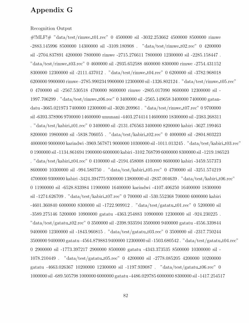
Appendix G

Recognition Output

#!MLF!# ”data/test/rimwe t01.rec” 0 4500000 sil -3032.253662 4500000 8500000 rimwe

-2883.145996 8500000 14300000 sil -3109.180908 . ”data/test/rimwe t02.rec” 0 4200000

sil -2704.837891 4200000 7800000 rimwe -2715.276611 7800000 12300000 sil -2285.158447 .

”data/test/rimwe t03.rec” 0 4600000 sil -2935.652588 4600000 8300000 rimwe -2754.431152

8300000 12300000 sil -2111.437012 . ”data/test/rimwe t04.rec” 0 6200000 sil -3782.968018

6200000 9900000 rimwe -2785.990234 9900000 12300000 sil -1326.802124 . ”data/test/rimwe t05.rec”

0 4700000 sil -2567.530518 4700000 8600000 rimwe -2805.017090 8600000 12300000 sil -

1997.706299 . ”data/test/rimwe t06.rec” 0 3400000 sil -2565.149658 3400000 7400000 gatan-

datu -3665.021973 7400000 12300000 sil -3020.209961 . ”data/test/rimwe t07.rec” 0 9700000

sil -6393.378906 9700000 14600000 umunani -4403.274414 14600000 18300000 sil -2383.268311

. ”data/test/kabiri t01.rec” 0 3400000 sil -2131.476563 3400000 8200000 kabiri -3627.199463

8200000 19800000 sil -5838.706055 . ”data/test/kabiri t02.rec” 0 4000000 sil -2804.803223

4000000 9000000 karindwi -3969.567871 9000000 10300000 sil -1011.013245 . ”data/test/kabiri t03.rec”

0 1900000 sil -1134.861694 1900000 6000000 kabiri -3102.768799 6000000 8300000 sil -1219.186523

. ”data/test/kabiri t04.rec” 0 4100000 sil -2194.458008 4100000 8600000 kabiri -3459.557373

8600000 10300000 sil -994.580750 . ”data/test/kabiri t05.rec” 0 4700000 sil -3251.574219

4700000 9300000 kabiri -3424.394775 9300000 13800000 sil -2837.004639 . ”data/test/kabiri t06.rec”

0 11900000 sil -6528.833984 11900000 16400000 karindwi -4107.406250 16400000 18300000

sil -1274.626709 . ”data/test/kabiri t07.rec” 0 700000 sil -530.552368 700000 6000000 kabiri

-4601.360840 6000000 8300000 sil -1722.909912 . ”data/test/gatatu t01.rec” 0 5200000 sil

-3589.275146 5200000 10900000 gatatu -4363.254883 10900000 12300000 sil -924.230225 .

”data/test/gatatu t02.rec” 0 3500000 sil -2398.933594 3500000 9400000 gatatu -4556.339844

9400000 12300000 sil -1843.960815 . ”data/test/gatatu t03.rec” 0 3500000 sil -2317.750244

3500000 9400000 gatatu -4564.879883 9400000 12300000 sil -1503.680542 . ”data/test/gatatu t04.rec”

0 2900000 sil -1773.397217 2900000 8500000 gatatu -4343.373535 8500000 10300000 sil -

1078.210449 . ”data/test/gatatu t05.rec” 0 4200000 sil -2778.085205 4200000 10200000

gatatu -4663.026367 10200000 12300000 sil -1197.939087 . ”data/test/gatatu t06.rec” 0

1000000 sil -689.505798 1000000 6000000 gatatu -4486.029785 6000000 8300000 sil -1417.254517

82

. ”data/test/gatatu t07.rec” 0 5300000 sil -3834.749268 5300000 11300000 gatatu -5677.827148

11300000 14300000 sil -2043.956055 . ”data/test/kane t01.rec” 0 3200000 sil -2327.186279

3200000 6600000 kane -2558.228760 6600000 9800000 sil -1841.534424 . ”data/test/kane t02.rec”

0 4500000 sil -2885.650391 4500000 8300000 kane -2810.858643 8300000 10300000 sil -1252.745239

. ”data/test/kane t03.rec” 0 2900000 sil -2006.716797 2900000 6700000 kane -2852.447510


3300000 7000000 kane -2733.631592 7000000 8300000 sil -725.258545 . ”data/test/kane t05.rec”

0 3200000 sil -1931.485962 3200000 6900000 kane -2699.544434 6900000 8300000 sil -746.918701

. ”data/test/kane t06.rec” 0 600000 sil -460.335510 600000 4300000 kane -3288.060059


7700000 11500000 kane -3384.530518 11500000 12300000 sil -540.977661 . ”data/test/gatanu t01.rec”

0 3300000 sil -2016.124268 3300000 10200000 gatanu -5082.707520 10200000 12300000 sil

-1063.003662 . ”data/test/gatanu t02.rec” 0 4100000 sil -2335.946777 4100000 10400000

gatanu -4572.570313 10400000 12300000 sil -990.890747 . ”data/test/gatanu t03.rec” 0

3300000 sil -1847.578735 3300000 9100000 gatanu -4382.743652 9100000 12300000 sil -1719.962524

. ”data/test/gatanu t04.rec” 0 4600000 sil -2818.372070 4600000 10100000 gatanu -3986.628174

10100000 12300000 sil -1200.381958 . ”data/test/gatanu t05.rec” 0 4100000 sil -2331.471924

4100000 9600000 gatanu -3933.541260 9600000 12300000 sil -1493.610840 . ”data/test/gatanu t06.rec”

0 900000 sil -576.625244 900000 6600000 gatandatu -5100.191895 6600000 8300000 sil -

1051.420288 . ”data/test/gatanu t07.rec” 0 6800000 sil -4709.265137 6800000 13900000

gatanu -5845.623535 13900000 14300000 sil -260.411957 . ”data/test/gatandatu t01.rec”

0 4300000 sil -3079.326416 4300000 9500000 gatandatu -4043.568359 9500000 12300000 sil

-1583.143311 . ”data/test/gatandatu t02.rec” 0 3500000 sil -1958.502197 3500000 10000000

gatandatu -5172.549805 10000000 12300000 sil -1294.331665 . ”data/test/gatandatu t03.rec”

0 3400000 sil -2035.299316 3400000 10100000 gatandatu -5445.789551 10100000 10300000 sil

-167.506531 . ”data/test/gatandatu t04.rec” 0 1800000 sil -1209.215454 1800000 8900000

gatandatu -5420.343750 8900000 12300000 sil -1944.851929 . ”data/test/gatandatu t05.rec”

0 5100000 sil -2798.036377 5100000 12300000 gatandatu -5575.925293 12300000 16300000

sil -2116.223145 . ”data/test/gatandatu t06.rec” 0 200000 sil -410.355652 200000 7800000

gatandatu -6987.959473 7800000 8300000 sil -381.262238 . ”data/test/gatandatu t07.rec” 0

10200000 sil -6375.278320 10200000 17300000 gatandatu -6801.508301 17300000 20300000

83

sil -1918.914795 . ”data/test/karindwi t01.rec” 0 3100000 sil -2471.800293 3100000 9600000

karindwi -5190.781250 9600000 10300000 sil -447.699554 . ”data/test/karindwi t02.rec” 0

4000000 sil -2909.214600 4000000 10300000 karindwi -4961.906250 10300000 14300000 sil

-2391.512451 . ”data/test/karindwi t03.rec” 0 3700000 sil -2514.477051 3700000 10200000

karindwi -5164.201172 10200000 14300000 sil -2367.164551 . ”data/test/karindwi t04.rec”

0 2200000 sil -1508.051147 2200000 8500000 karindwi -4925.602539 8500000 12300000 sil

-2103.998535 . ”data/test/karindwi t05.rec” 0 3100000 sil -1962.216675 3100000 9400000

karindwi -5152.186035 9400000 12300000 sil -1768.007935 . ”data/test/karindwi t06.rec”

0 1500000 sil -1065.677124 1500000 7200000 karindwi -5150.283203 7200000 9800000 sil -

1699.175293 . ”data/test/karindwi t07.rec” 0 6100000 sil -4322.256348 6100000 11800000

karindwi -5017.796387 11800000 18300000 sil -4314.830078 . ”data/test/umunani t01.rec”

0 2100000 sil -1265.518921 2100000 8500000 umunani -4985.961426 8500000 10300000 sil

-1060.763550 . ”data/test/umunani t02.rec” 0 2700000 sil -1435.257080 2700000 10000000

umunani -5558.234863 10000000 10300000 sil -197.015854 . ”data/test/umunani t03.rec” 0

3400000 sil -1931.043823 3400000 10400000 umunani -5685.582520 10400000 12300000 sil


umunani -5220.315430 9400000 11800000 sil -1374.329956 . ”data/test/umunani t05.rec”

0 2500000 sil -1402.714966 2500000 9500000 umunani -5534.970215 9500000 12300000 sil


umunani -7357.295898 12400000 14300000 sil -1438.931641 . ”data/test/umunani t07.rec”

0 7800000 sil -5594.510254 7800000 16700000 umunani -7102.675293 16700000 18300000

sil -982.074829 . ”data/test/icyenda t01.rec” 0 1900000 sil -1452.497437 1900000 7700000

icyenda -4527.358398 7700000 10300000 sil -1541.053589 . ”data/test/icyenda t02.rec” 0

1800000 sil -1142.076294 1800000 7300000 icyenda -4290.866211 7300000 8300000 sil -662.530518

. ”data/test/icyenda t03.rec” 0 4100000 sil -2891.251953 4100000 8300000 icyenda -3231.903564

8300000 11800000 sil -2064.225830 . ”data/test/icyenda t04.rec” 0 2100000 sil -1223.421631

2100000 8100000 icyenda -4642.086426 8100000 10300000 sil -1201.611450 . ”data/test/icyenda t05.rec”

0 3400000 sil -2206.691406 3400000 9000000 icyenda -4240.103027 9000000 12300000 sil -

1832.621826 . ”data/test/icyenda t06.rec” 0 800000 sil -518.711365 800000 7700000 gatan-

datu -6347.489746 7700000 10300000 sil -1752.465698 . ”data/test/icyenda t07.rec” 0 12400000

sil -8788.501953 12400000 19300000 icyenda -6196.111328 19300000 24300000 sil -3499.174805

84

. ”data/test/zero t01.rec” 0 1600000 sil -915.991943 1600000 6400000 zero -3366.200684

6400000 8300000 sil -1075.914063 . ”data/test/zero t02.rec” 0 2900000 sil -1598.527100

2900000 7700000 zero -3288.929688 7700000 8300000 sil -425.674469 . ”data/test/zero t03.rec”

0 2500000 sil -1701.465332 2500000 7300000 zero -3282.274902 7300000 8300000 sil -527.153931

. ”data/test/zero t04.rec” 0 3500000 sil -2084.071045 3500000 8000000 zero -3044.202148

8000000 10300000 sil -1241.999268 . ”data/test/zero t05.rec” 0 2800000 sil -1659.132935

2800000 7300000 zero -3011.566162 7300000 8300000 sil -530.568054 . ”data/test/zero t06.rec”

0 7200000 sil -4286.444336 7200000 10400000 zero -2708.985840 10400000 12300000 sil -

1289.067627 . ”data/test/zero t07.rec” 0 8000000 sil -5543.634766 8000000 12700000 zero

-4128.586914 12700000 18300000 sil -3445.831787 .

85

appendix H

Testing Data

data/test/rimwe t01.MFC







data/test/kabiri t01.MFC







data/test/gatatu t01.MFC







data/test/kane t01.MFC







86

data/test/gatanu t01.MFC







data/test/gatandatu t01.MFC







data/test/karindwi t01.MFC







data/test/umunani t01.MFC







data/test/icyenda t01.MFC



87





data/test/zero t01.MFC







88

automatic speech recognition: human computer interface for kinyarwanda language

Documents