AUTOMATIC CONTRAST ENHANCEMENT BY HISTOGRAM WARPING

Mark Grundland and Neil A. Dodgson Computer Laboratory, University of Cambridge Cambridge, United Kingdom Mark @ Eyemaginary.com

Abstract: We present an automated algorithm for global contrast enhancement of images with multimodal histograms. To locate modes and valleys, histogram analysis is performed by kernel density estimation, a robust nonparametric statistical method. Histogram warping by monotonic splines pushes the modes apart, spreading them out more evenly across the dynamic range. This technique can assist in the contrast correction of images taken facing the light source.

Keywords: Image enhancement, contrast enhancement, histogram modification, histogram equalization, mode detection, kernel density estimation, monotonic splines.

1. INTRODUCTION

Automatic contrast enhancement by global histogram modification is a basic tool of image enhancement [1,2] for visual inspection. It is commonly used in digital photography, remote sensing, medical imaging, and scientific visualization. The task calls for finding an appropriate balance between emphasis and distortion. Contrast enhancement makes images easier to interpret by making object features easier to distinguish. The classical image segmentation techniques, clustering and thresholding, assume that the shades that differentiate object features are less common than those that comprise them. Hence the modes of the image histogram reflect the similarities within uniformly colored object features while the valleys record the characteristics that distinguish them. Our histogram warping technique improves the contrast between object features by spreading apart the modes of an image histogram to take better advantage of the entire dynamic range. It addresses the need for a robust, generally applicable, contrast enhancement algorithm

2 Mark Grundland and Neil A. Dodgson

for images with multimodal histograms. Our algorithm (Figure 1) improves the contrast of photographs with both strong highlights and pronounced shadows. In particular, it can handle contrast correction of images taken with the camera facing the sun, which has long been a challenge for photography.

Our input is a gray level image with n pixel values [0,1]ix ∈ with a unit dynamic range, having an implied probability density ( )f x with cumulative distribution ( )F x and quantiles 1( )F x− . If an importance map is available, it defines pixel weights iw such that iw n∑ = , otherwise all 1iw = .

1.1 Previous Work

Global contrast enhancement is performed by a spatially invariant, gray level transformation ( )y T x= . Contrast stretch [1,2] by a linear transforma-tion, defined to satisfy 1( ( ))T Fτ τ−= and 11 ( (1 ))T Fτ τ−− = − , can only be effective as long as the image doesn’t already span the dynamic range. Other parametric transformations [1-3], such as gamma correction, also lack the flexibility to adapt to multimodal histograms. Histogram thinning [4-6], robustly implemented via a mean shift procedure [7], shifts each gray level towards its nearest histogram mode. Histogram thinning improves the con-trast between object features but only by reducing the contrast within them since the modes of the histogram are not redistributed across the dynamic range. Histogram equalization [1-3,8], defined by 1( ( ))y T F y−= with

Figure 1. Contrast enhancement of images (left) by our histogram warping technique (right).

Automatic Contrast Enhancement by Histogram Warping 3

( ) ( )T x F x= , produces an approximately uniform gray level distribution. Notorious for excessive distortion, it entirely eliminates histogram modes, which risks reducing the contrast between object features. Configuring the process [9] to accommodate multimodal histograms may demand skillful user intervention. There have been attempts to partition the histogram by the mean [10], the median [11], the minimal error split [12], the recursive means [13], and the histogram valleys [14] in order to separately apply histogram equalization to each histogram region. They are all susceptible to visible defects since the transformation is not continuously differentiable across histogram regions. Histogram warping overcomes this common deficiency in order to improve the visual quality of contrast enhancement. By using robust statistics, we also improve the reliability of contrast enhancement. To allow global contrast enhancement to take account of local image structure [15], our method supports the use of an edge map [16] as an importance map. To provide for local contrast enhancement [17], it is also compatible with the partially overlapped sub-block histogram modification procedure [18].

2. OUR TECHNIQUE

2.1 Histogram Transformation

Our histogram warping transformation ( )y T x= is defined by a mapping of corresponding gray level values ( )k kb T a= and their contrast adjustments

( )k kd T a′= . Thus, we can locally control how the histogram is shifted k ka b≠ , compressed 0 1kd≤ < , or stretched 1kd > . We require only that

the sequence ka is strictly increasing, kb is increasing, and kd is finite and nonnegative. A continuously differentiable 1C transformation is needed in order to avoid artificial discontinuities in the resulting histogram

( )

1 1 1( ( )) ( ( ))f T y T T y− − −′ . So, for best image quality, piecewise exponential [6] and piecewise linear [1,8] histogram transformations should be avoided unless efficiency is the overriding concern. The transformation should be monotonic ( ) 0T x′ ≥ to preserve the natural order of gray levels so that the polarity of the image is not reversed. For instance, the commonly used cubic spline [3] histogram transformations may fail to be monotonic in regions of heightened contrast 3k kd r> . Hence, we base our histogram warping method on a piecewise rational quadratic, 1C interpolating monotonic spline [19,20]:

( )( ) ( ) ( )

21

1 11

1( )

2 1k k

k k kk k k k

r t d t tT x b b b

r d d r t t−

− −−

+ −= + −

+ + − −, (1)

with 1

1

k kk

k k

b bra a

−

−

−=

− and 1

1

k

k k

x ata a

−

−

−=

− for 1[ , ]k kx a a−∈ .

4 Mark Grundland and Neil A. Dodgson 2.2 Histogram Analysis

Our model assumes that each mode of the histogram corresponds to an object feature in the image. For instance, a bimodal histogram often reflects the distinction between foreground and background features. The extent of each object feature, in the spatial domain as well as in the dynamic range, is determined by the span of its mode in the histogram, the interval between the adjoining valleys of the histogram. To reduce the impact of image noise and quantization on the analysis of the structure of the grey level distribution, we apply kernel density estimation [21] in place of ad hoc approaches [4,5,14]. If speed is critical, a random subset of the data can be used. We approximate the density ( )f x as a mixture of Gaussians centered on the observations ix :

( )3

1( ) ( )

1( ) ( )

ii

i

ii i

i

x xf x w Gnh h

x xf x w x x Gnh h

−=

−′ = −

∑

∑ with

2

2( )

2

x

eG xπ

−

= . (2)

As more computationally efficient truncated kernels could cause spurious ripples, the infinite support of the Gaussian kernel ( )G x is needed to ensure that the density estimate remains smooth. To minimize estimation error, the optimal bandwidth 1 5O( )h n−= for the density estimate ( )f x can afford to be more sensitive to the data than the optimal bandwidth 1 7O( )h n−= for the derivative estimate ( )f x′ required in mode detection. As the bandwidth h increases, the estimate’s bias increases and its variance decreases while the estimated density becomes smoother and its modes fewer. A conservative bandwidth ensures no more modes are detected than would be observed in an asymptotically optimal density estimate. Using this maximal smoothing principle [22], we select the largest degree of smoothing compatible with the interquartile range, ( ) ( )1 1 1 73 1

4 40.7816774 ( ) ( )h F F n− − −= − . Next, we locate the histogram valleys. We consider a critical point

( ) 0f v′ = to be a legitimate valley when it has a span of at least 2δ , where ( ) 0f u′ < when [ , )u v v−∈ and ( ) 0f w′ > when ( , ]w v v+∈ for

1 1[ , ] [ ( ( ) ), ( ( ) )]v v F F v F F vδ δ− −− + = − + . Density estimates based on a symmetric kernel are not reliable near the endpoints of the data range, so we do not look for critical points among the outliers, requiring ( ) 1F vδ δ≤ ≤ − . We start the search by partitioning the data range into equiprobable intervals. Each interval [ , ]u w spans ( ) ( )F w F uδ = − , so it can contain at most one legitimate valley. When an interval’s boundaries satisfy the valley condition, its valley can be quickly located by bisection: compute the midpoint

( ) 2v u w= + and move the lower limit u v← when ( ) 0f v′ < or move the upper limit w v← when ( ) 0f v′ > . To eliminate the possibility of a ripple on an inflection or a plateau, we optionally verify the valley condition on

Automatic Contrast Enhancement by Histogram Warping 5 [ , ]v v− + by confirming that this interval contains no modes. We use the mean shift procedure [7], a mode seeking gradient ascent method with step size adapted to the density estimate. The candidate v is indeed a valid valley if, when starting at either side of the valley, the procedure does not monotonically converge on a mode before leaving the interval [ , ]x v v− +∈ :

1 ( )( )

ii i

i

x xx w x Gnhf x h

−← ∑ starting at 1

2 mini

ix vx v v x

≠= ± − . (3)

2.3 Histogram Mapping

The histogram valleys kv segment the dynamic range 1 1[ , ] [0,1]Kv v − = into object features 1[ , ]k kv v− . When no valleys are detected, as a unimodal histogram is often caused by the overlap of a pair of object features, we treat the mode [7] as though it were a valley, splitting the histogram into light and dark regions. Enhancing an object’s contrast by applying histogram equalization to its entire histogram region still poses the risk of unwarranted distortion. While a more equitable histogram may indeed have a flatter shape, entirely flattening the mode of each histogram region can inordinately enhance noise in uniformly colored areas of the image. Instead, in our histogram mapping ( )k kb T a= , each object feature is represented by the midpoint ( )1 2k k ka v v−= + of its histogram region and equalization

( ) ( )( ) ( )1 1 1( ) ( ) ( ) ( ) ( ) ( )k k k k k k k k kb F v F a v F a F v v F v F v− − −= − + − − is only applied to the midpoint. Equating relative gray level with relative probability ( ) ( ) ( ) ( )1 1 1 1( ) ( ) ( ) ( )k k k k k k k kb v v v F a F v F v F v− − − −− − = − − , our mapping displaces each midpoint toward the less probable side of its histogram region, so k kb a< whenever 1( ) ( ) ( ) ( )k k k kF a F v F v F a−− < − . Enhancing detail without undue distortion, our midpoint mapping gives greater emphasis to the more common gray levels of an object feature while limiting the scope of gray level shift ( )1 2k k k kb a v v −− ≤ − . The more probable side of a histogram region tends to be stretched at the expense of compressing the less probable side. Because a mode is typically found on the more probable side of its histogram region, the mapping tends to shift modes away from each other, spreading them out more evenly across the dynamic range.

To enhance images that make use of only a small portion of the dynamic range, we have incorporated standard histogram stretching into our mapping. Thus, we map the data range 1 1

0 1[ , ] [ (0), (1)]Ka a F F− −+ = to the dynamic

range 0 1[ , ] [0,1]Kb b + = and compress the outliers by stretching the rest of the histogram from 1 1

1[ , ] [ ( ), (1 )]Ka a F Fτ τ− −= − to 1[ , ] [ ,1 ]Kb b τ τ= − . By not mapping any gray levels out of gamut, our approach averts information loss. Finally, we discard any outliers from our previously calculated mapping to ensure that 1 1[ ( ), (1 )]ka F Fτ τ− −∈ − and [ ,1 ]kb τ τ∈ − for all 1 k K≤ ≤ .

6 Mark Grundland and Neil A. Dodgson

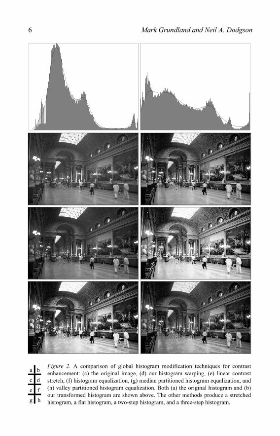
Figure 2. A comparison of global histogram modification techniques for contrast enhancement: (c) the original image, (d) our histogram warping, (e) linear contrast stretch, (f) histogram equalization, (g) median partitioned histogram equalization, and (h) valley partitioned histogram equalization. Both (a) the original histogram and (b) our transformed histogram are shown above. The other methods produce a stretched histogram, a flat histogram, a two-step histogram, and a three-step histogram.

a b

c d

e f

g h

Automatic Contrast Enhancement by Histogram Warping 7 2.4 Histogram Contrast

The local stretching or compression of the histogram is dictated by the contrast adjustments ( )k kd T a′= . To avoid creating unwarranted spikes or holes in the histogram, we limit the degree of distortion to 1

kdλ λ− ≤ ≤ . Experiments with a variety of formulations lead us to apply the principles of histogram equalization to extend a derivate formula for monotonic splines [20]. Each contrast adjustment reflects a compromise between a left side slope and a right side slope. We rely on the geometric mean of the slopes weighted by the probability mass of the slopes’ intervals. The geometric mean ( )

1 2( , )s s s sΦ − + − += has the benefit of preserving flat slopes ( ,0) 0sΦ = while canceling inverse slopes 1( , ) 1s sΦ − = . To obtain the local slopes, we consider mapping local medians 1

1( ( ) 2 ( ) 2)k k ka F F a F a−±±= + to local

midpoints ( )1 2k k kb b b±±= + . Hence, along with the endpoints 0 0 0d b a+ +=

as well as ( ) ( )1 1 11 1K K Kd b a− −+ + += − − , the contrast adjustments are defined:

1 1

1 1 1 1

( ) ( ) ( ) ( )( ) ( ) ( ) ( )

k k k kk k k k

F a F a F a F aF a F a F a F a

k k k kk

k k k k

b b b bda a a a

− +

+ − + −

− −− +− −

− +

− −= − −

. (4)

3. RESULTS AND DISCUSSION

We applied our histogram warping method to various stock photographs. All our experiments used analysis resolution 0.02δ = , outlier threshold

0.01τ = , and distortion limit 5λ = . The results did not appear particularly sensitive to these parameter values. In Figure 2, we illustrate an image for which linear contrast stretch makes little difference while histogram equali-zation methods prove excessive (note how equalization makes the people look as bright as the lamps while the floor and skylight suffer apparent distortion). Our algorithm spreads out the central modes of the histogram to more evenly occupy the dynamic range, without overly altering the relative proportions of light and dark tones. Because its design combines aspects of linear contrast stretch with histogram equalization, our technique appears to balance the limited distortion of the former with the detail emphasis of the latter. Our experience suggests that where one of these standard approaches fares well, our technique does also. Where both fall short, our technique often yields a visible improvement. In such cases, as in Figure 1, we can reveal hidden detail by enhancing the contrast of the midtones despite the strong presence of both highlights and shadows. The advantage of histogram warping by 1C monotonic splines is that it avoids the defects caused by the abrupt transitions between histogram stretching and compression that arise in previously proposed piecewise histogram transformations [1,4-6,8-14].

8 Mark Grundland and Neil A. Dodgson REFERENCES

1. Gonzalez, R. C. and Woods, R. E. 2002. Digital Image Processing, 2 ed. Prentice Hall. 2. Zamperoni, P. 1995. Image Enhancement. Advances in Imaging and Electron Physics, 92,

1-77. 3. O'Gorman, L. and Brotman, L. S. 1985. Entropy-Constant Image Enhancement by

Histogram Transformation. Proceedings of SPIE, 575, 106-113. 4. Rosenfeld, A. and Davis, L. S. 1978. Iterative Histogram Modification. IEEE Transactions

on Systems, Man & Cybernetics, 8, 4, 300-302. 5. Peleg, S. 1978. Iterative Histogram Modification 2. IEEE Transactions on Systems, Man &

Cybernetics, 8, 7, 555-556. 6. Raji, A., Thaibaoui, A., Petit, E., et al. 1998. A Gray-Level Transformation-Based Method

for Image Enhancement. Pattern Recognition Letters, 19, 13, 1207-1212. 7. Cheng, Y. 1995. Mean Shift, Mode Seeking, and Clustering. IEEE Transactions on

Pattern Analysis & Machine Intelligence, 17, 8, 790-799. 8. Sang-Yeon, K., Dongil, H., Seung-Jong, C., et al. 1999. Image Contrast Enhancement

Based on the Piecewise-Linear Approximation of CDF. IEEE Transactions on Consumer Electronics, 45, 3, 828-834.

9. Dale-Jones, R. and Tjahjadi, T. 1992. Four Algorithms for Enhancing Images with Large Peaks in Their Histogram. Image & Vision Computing, 10, 7, 495-507.

10. Yeong-Taeg, K. 1997. Contrast Enhancement Using Brightness Preserving Bi-Histogram Equalization. IEEE Transactions on Consumer Electronics, 43, 1, 1-8.

11. Yu, W., Qian, C., and Baeomin, Z. 1999. Image Enhancement Based on Equal Area Dualistic Sub-Image Histogram Equalization Method. IEEE Transactions on Consumer Electronics, 45, 1, 68-75.

12. Soong-Der, C. and Ramli, A. R. 2003. Minimum Mean Brightness Error Bi-Histogram Equalization in Contrast Enhancement. IEEE Transactions on Consumer Electronics, 49, 4, 1310-1319.

13. Soong-Der, C. and Ramli, A. R. 2003. Contrast Enhancement Using Recursive Mean-Separate Histogram Equalization for Scalable Brightness Preservation. IEEE Transactions on Consumer Electronics, 49, 4, 1301-1309.

14. Young-Ho, K., Hyun-Suk, J., Kun-Sop, K., et al. 1998. Region-Based Histogram Specification for Dynamic Range Expansion. Proceedings of SPIE, 3302, 90-97.

15. Leu, J.-G. 1992. Image Contrast Enhancement Based on the Intensities of Edge Pixels. CVGIP: Graphical Models & Image Processing, 54, 6, 497-506.

16. Weszka, J. S. and Rosenfeld, A. 1979. Histogram Modification for Threshold Selection. IEEE Transactions on Systems, Man & Cybernetics, 9, 1, 38-52.

17. Pizer, S. M., Amburn, E. P., Austin, J. D., et al. 1987. Adaptive Histogram Equalization and Its Variations. Computer Vision, Graphics, & Image Processing, 39, 3, 355-368.

18. Joung-Youn, K., Lee-Sup, K., and Seung-Ho, H. 2001. An Advanced Contrast Enhancement Using Partially Overlapped Sub-Block Histogram Equalization. IEEE Transactions on Circuits & Systems for Video Technology, 11, 4, 475-484.

19. Gregory, J. A. and Delbourgo, R. 1982. Piecewise Rational Quadratic Interpolation to Monotonic Data. IMA Journal of Numerical Analysis, 2, 123-130.

20. Sarfraz, M., Al-Mulhem, M., and Ashraf, F. 1997. Preserving Monotonic Shape of the Data Using Piecewise Rational Cubic Functions. Computers & Graphics, 21, 1, 5-14.

21. Scott, D. W. 1992. Multivariate Density Estimation: Theory, Practice, and Visualization. Wiley.

22. Terrell, G. R. 1990. The Maximal Smoothing Principle in Density Estimation. Journal of the American Statistical Association, 85, 410, 470-477.