Automatic calculation of total lung capacity from automatically traced lung boundariesin postero-anterior and lateral digital chest radiographsFrancisco M. Carrascal, José M. Carreira, Miguel Souto, Pablo G. Tahoces, Lorenzo Gómez, and Juan J. Vidal Citation: Medical Physics 25, 1118 (1998); doi: 10.1118/1.598303 View online: http://dx.doi.org/10.1118/1.598303 View Table of Contents: http://scitation.aip.org/content/aapm/journal/medphys/25/7?ver=pdfcov Published by the American Association of Physicists in Medicine Articles you may be interested in Development and evaluation of a computer-aided diagnostic scheme for lung nodule detection in chestradiographs by means of two-stage nodule enhancement with support vector classification Med. Phys. 38, 1844 (2011); 10.1118/1.3561504 Automated lung segmentation in digital lateral chest radiographs Med. Phys. 25, 1507 (1998); 10.1118/1.598331 Automated segmentation of anatomic regions in chest radiographs using an adaptive-sized hybrid neural network Med. Phys. 25, 998 (1998); 10.1118/1.598277 Automated lung segmentation in digital posteroanterior and lateral chest radiographs: Applications in diagnosticradiology and nuclear medicine Med. Phys. 24, 2056 (1997); 10.1118/1.598137 Computerized analysis of interstitial disease in chest radiographs: Improvement of geometric-pattern featureanalysis Med. Phys. 24, 915 (1997); 10.1118/1.598012

Automatic calculation of total lung capacity from automatically traced lungboundaries in postero-anterior and lateral digital chest radiographs

Francisco M. Carrascal,a) Jose M. Carreira, and Miguel SoutoDepartment of Radiology, University of Santiago, Spain (Complejo Hospitalario Universitario de Santiago)

Pablo G. Tahoces and Lorenzo GomezDepartment of Electronics and Computer Science, University of Santiago, Spain

Juan J. VidalDepartment of Radiology, University of Santiago, Spain (Complejo Hospitalario Universitario de Santiago)

~Received 28 October 1996; accepted for publication 30 April 1998!

Total lung capacity~TLC! is a very important parameter in the study of pulmonary function. In thepulmonary function laboratory, it is normally obtained using plethysmography or helium dilutiontechniques. Several authors have developed methods of calculating the TLC using postero-anterior~PA! and lateral chest radiographs. These methods have not been often used in clinical practice. Inthe present work, we have developed an automated computer-based method for the calculation ofTLC, by determining the pulmonary contours from digital PA and lateral radiographs of the thorax.The automatic tracing of the pulmonary borders is carried out using:~1! a group of reference linesis determined in each radiograph;~2! a family of rectangular regions of interest~ROIs! defined,which include the pulmonary borders, and in each of them the pulmonary border is identified usingedge enhancement and thresholding techniques;~3! removing outlaying points from the preliminaryboundary set; and~4! the pulmonary border is corrected and completed by means of interpolation,extrapolation, and arc fitting. The TLC is calculated using a computerized form of the radiographicellipses method of Barnhard. The pulmonary borders were automatically traced in a total of 65normal radiographs~65 PA and 65 lateral views of the same patients!. Three radiologists carried outa subjective evaluation of the automatic tracing of the pulmonary borders, with a finding of no erroror only one minor error in 67.7% of the PA evaluations, and in 75.9% of the laterals. Comparing theautomatically traced borders with borders traced manually by an expert radiologist, we obtained aprecision of 0.99060.001 for the PA view, and 0.98560.002 for the lateral. The values of TLCobtained by the automatic calculation described here showed a high correlation (r 50.98) withthose obtained by applying the manual Barnhard method. ©1998 American Association of Physi-cists in Medicine.@S0094-2405~98!01307-8#

Key words: digital chest images, computer-aided diagnosis, CAD, total lung capacity, TLC

I. INTRODUCTION

Total lung capacity~TLC! is an important parameter whenstudying pulmonary function. It is normally obtained in thepulmonary function laboratory. It cannot be calculated bysimple spirometric methods, but is obtained using more ex-pensive, complex methods such as plethysmography or he-lium dilution techniques. Various authors have developedmethods to calculate of TLC using postero-anterior~PA! andlateral chest radiographs at full inspiration, which are a rou-tine part of the clinical examination.1–6 Using radiologicmethods has the advantage of avoiding TLC measurement inthe pulmonary function laboratory, without additional cost orradiologic exposure of the patient. There are two differentversions of the radiographic method. The first considers thatthe cross section of the thorax is elliptical.1–4 In this case theTLC is the difference between the total thoracic volume~TTV! and the sum of the nongas containing volume of thethorax ~NCV!, the blood volume~BV!, and the pulmonarytissue volume ~TV!. Thus TLC5TTV-NCV-BV-TV. 1–4

TTV is calculated by summing the volumes of the elliptical

cylindroids whose major and minor axes are defined as thedistances between the pulmonary borders of the PA and lat-eral radiographs, respectively. The NCV is calculated byadding the volume of the heart and of the hemidiaphragmsconsidered as ellipsoids. The BV and the TV are obtainedfrom the height and weight of the patient according to pre-established formulae.2 The second version of the radio-graphic method of determining the TLC, the planimetricmethod, deduces volumes from pulmonary areas by means ofan empirical formula: TLC~in cm3)58.53RLA21200,where RLA, the ‘‘radiographic lung area’’ in cm2, is the sumof the thoracic areas measured with a planimeter in the PAand lateral radiographs.5,6

Both methods are based upon the prior identification ofthe pulmonary borders in PA and lateral radiographs of thethorax. Originally, the boundary was traced by a human op-erator, who also identified and measured the distances orareas.1–6 Later, semiautomatic methods began to be de-scribed, in which the pulmonary borders were traced manu-ally, then the information was entered into a computer forprocessing.7–9 In 1974, Paulet al. developed a fully auto-

1118 1118Med. Phys. 25 „7…, July 1998, Part 1 0094-2405/98/25 „7…/1118/14/$10.00 © 1998 Am. Assoc. Phys. Med.

mated method, where the pulmonary borders were identifiedautomatically in digitized radiographs, using image process-ing techniques.10 Until now, only semi-automatic methodshave been used to calculate TLC in screenings designed todetermine predictive equations and normal values within apopulation survey.11,12

The advances made in the automatic detection of pulmo-nary borders related to systems of computer-assisted diagno-sis ~CAD! or projects for radiographic optimization,13–18

have not been accompanied by any increased or improvedutilization in the calculation of TLC. Thus McNitt-Grayet al.13 developed a technique for automatic segmentation ofthoracic images, obtaining an overall precision of 76%; Dur-yea and Boone14 developed an algorithm for the segmenta-tion of the pulmonary fields in digital radiographs of thethorax, obtaining an average precision of 0.95760.003 forthe right lung, and 0.96060.003 for the left; Xu and Doi15 asa continuation of the work of Powellet al.16 and Nakamoriet al.,17 developed a method for the determination of the rib-cage boundary on PA radiographs, with a moderate to highlyaccurate results in 96% of the 1000 cases examined; andArmato et al.18 developed a technique to detect asymmetryin digital chest radiographs, obtaining a sensitivity of 91%and a specificity of 80% in 70 chest images.

In this article we describe an automatic CAD method forthe lung boundary detection and the calculation of TLC, us-ing digital chest radiographs. The TLC is calculated using avariant of the method of ellipses of Barnhardet al.1 Themethod has been tested on radiographs of 65 normal sub-jects.

II. MATERIALS AND METHODS

A. Materials

A total of 65 cases was used, each case consisting of tworadiographs, one PA and one lateral, in vertical orientation(14317 in.), correctly centered, and at full inspiration. Allthe images were obtained with high kilovoltage~145 KV!,and an AIR-GAP anti-diffusion technique which produces amagnification of 10%.19,20 The radiographs were taken of to29 males and 36 females ranging in age from 18 to 83 years.The digital images of all radiographs were obtained using aKDRF-S scanner~Konica Corp., Tokyo, Japan! with a pixelsize of 0.175 mm and a 10-bit gray scale. These digitizedimages were converted to an 8-bit gray-level scale and aspatial resolution of 0.875 mm per pixel, giving a 4003486 pixel image. The images were interpolated down, andtheir dynamic range reduced for computer purposes, and toeliminate high spatial frequencies and peaks that could affectthe edge detection algorithms used. Smaller images and dy-namic ranges were not used because they would have pro-duced reduced sets of points for the interpolation algorithms.A VAX 4000-300~Digital Equipment Corp., Maynard, MA!,under the VMS operating system, was used for all calcula-tions. The computer programs were written in FORTRANand IDL. Copies of the digital radiographs were printed onradiographic film using a Matrix Compact L laser printer~Agfa Gevaert N.V., Mortsel, Belgium!.

B. Overall scheme

Barnhard et al.1 made the assumption that the cross-sectional shape of the lung is elliptical, and that the lungsmay be represented as a series of elliptical cylindroids. Inorder to calculate the lung volumes, it is necessary to obtainthe lung borders and to use a computerized algorithm. In themanual and semiautomatic methods, the pulmonary bordersare traced manually. Our algorithm detects the lung edgesautomatically, and follows in many respects the samescheme as the automatic version of Paulet al.10 Figure 1shows its general outline of operation.

C. Automatic tracing of pulmonary borders

1. Definition of reference lines and detection of theposterior pulmonary border

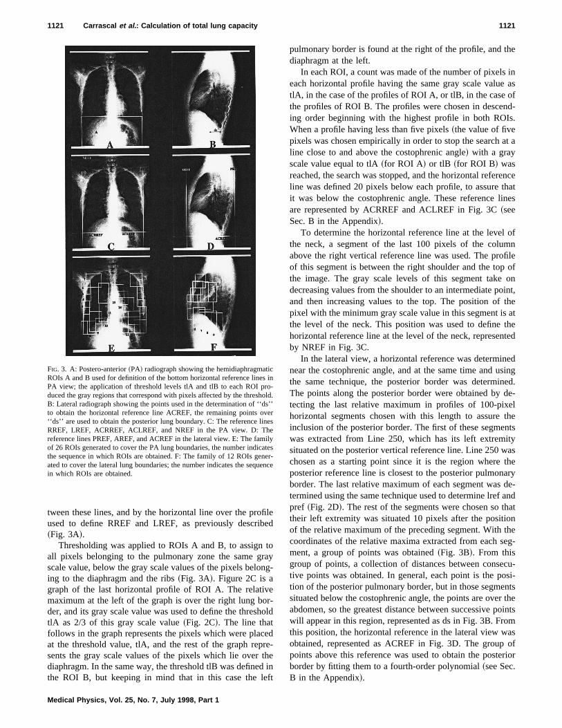
Vertical and horizontal lines of reference were determinedby means of processing profiles of gray levels in horizontalsmoothed image lines~Fig. 2, A–D!. Five reference lineswere defined in the PA radiograph: two vertical, one on eachside of the thorax, one horizontal at the level of the neck, andtwo horizontal at the level of each costophrenic angle. Threelines of reference were defined in the lateral radiographs: twovertical, one anterior, and one posterior, both situated at thethoracic walls, and one horizontal at the costophrenic angle~Fig. 3, A–D!.

In the PA view, the left and right references were definedthrough the detection of the first and last relative maxima inhorizontal profiles represented by rref and lref in the typicalprofile shown in Fig. 2A. An 8 pixel wide smoothing maskwas applied to the profile to eliminate small relative maximawhich could affect the detection of rref and lref. These werefound by studying the change of sign from positive to nega-tive in the first derivative of the profile. Successive profileswere examined in descending order beginning with level250, which was chosen as a starting point because its profile

FIG. 1. General scheme of the lung boundary detection and TLC calculationprocedure.

1119 Carrascal et al. : Calculation of total lung capacity 1119

Medical Physics, Vol. 25, No. 7, July 1998, Part 1

is always over the lung region. In each profile a position wasfound in the region of the mediastinum, mref in Fig. 2A, bystudying the change in sign from negative to positive in thesecond derivative of the profile. In each profile, the distancebetween the right pulmonary border and the mediastinumwas determined by the number of pixels between the posi-tions of rref and mref~Fig. 2A!. By analyzing the profiles indescending order, one arrives at a profile, located above thediaphragm, where the distance previously described is lessthan 30 pixels. From the positions of the right and left bor-ders obtained in this profile~rref and lref! the vertical lines ofreference of the PA view were defined, 10 pixels before and10 pixels after the positions of the right and left borders ofthe profile, respectively, so that they do not intersect thepulmonary region. These lines of reference are representedby RREF and LREF in Fig. 3C~see Sec. A in the Appendix!.

The posterior and anterior lines of reference, in the lateralview, were defined according to the first and last relativemaxima in the profiles of the center of the image. The 10horizontal profiles in the center of the image were chosenbecause they always lie within the pulmonary region. In eachof these profiles, the positions of the first and last relative

maxima, represented by aref and pref in the typical profileshown in Fig. 2B, were determined by a procedure similar tothat used for rref and lref, as described earlier. In each groupof 10 relative maxima, a mean and its standard deviationwere determined. In the group of the 10 aref values, that onewas chosen which had the least value between the mean andthe mean minus the standard deviation of the group. Theanterior line of reference, represented as AREF in Fig. 3D,was defined substracting 20 pixels to this value. In the groupof the 10 pref values, that one was chosen which had thegreatest value between the mean and the mean plus the stan-dard deviation of the group. The posterior line of reference,represented as PREF in Fig. 3D, was defined adding 20 pix-els to this value. The separation of 20 pixels was used toassure that the lines of reference would not intersect the pul-monary region~see Sec. A in the Appendix!.

The horizontal lines of reference at the costophrenicangles in the PA view were obtained in two ROIs whichcover the diaphragmatic regions of both lungs, ROIs A and Bin Fig. 3A. ROIs A and B were delimited by the lower partof the image, by the reference lines LREF and PREF, by theline of separation between A and B which is halfway be-

FIG. 2. A: Gray level profile of a typical horizontal PA image line through the lung, showing the points rref, mref, and lref, used for definition of verticalreference lines RREF and LREF in the PA view. B: Gray level profile of a typical horizontal lateral image line through the lung, showing the points aref andpref, used for definition of vertical reference lines AREF and PREF in the lateral view. C: Post-thresholding gray level profile of a typical horizontal imageline through the right hemidiaphragmatic ROI A, showing the threshold level tlA, used for definition of the right bottom horizontal reference line ACRREFin the PA view. D: Typical SOI profile showing the detected point of the posterior boundary marked by an arrow.

1120 Carrascal et al. : Calculation of total lung capacity 1120

Medical Physics, Vol. 25, No. 7, July 1998, Part 1

tween these lines, and by the horizontal line over the profileused to define RREF and LREF, as previously described~Fig. 3A!.

Thresholding was applied to ROIs A and B, to assign toall pixels belonging to the pulmonary zone the same grayscale value, below the gray scale values of the pixels belong-ing to the diaphragm and the ribs~Fig. 3A!. Figure 2C is agraph of the last horizontal profile of ROI A. The relativemaximum at the left of the graph is over the right lung bor-der, and its gray scale value was used to define the thresholdtlA as 2/3 of this gray scale value~Fig. 2C!. The line thatfollows in the graph represents the pixels which were placedat the threshold value, tlA, and the rest of the graph repre-sents the gray scale values of the pixels which lie over thediaphragm. In the same way, the threshold tlB was defined inthe ROI B, but keeping in mind that in this case the left

pulmonary border is found at the right of the profile, and thediaphragm at the left.

In each ROI, a count was made of the number of pixels ineach horizontal profile having the same gray scale value astlA, in the case of the profiles of ROI A, or tlB, in the case ofthe profiles of ROI B. The profiles were chosen in descend-ing order beginning with the highest profile in both ROIs.When a profile having less than five pixels~the value of fivepixels was chosen empirically in order to stop the search at aline close to and above the costophrenic angle! with a grayscale value equal to tlA~for ROI A! or tlB ~for ROI B! wasreached, the search was stopped, and the horizontal referenceline was defined 20 pixels below each profile, to assure thatit was below the costophrenic angle. These reference linesare represented by ACRREF and ACLREF in Fig. 3C~seeSec. B in the Appendix!.

To determine the horizontal reference line at the level ofthe neck, a segment of the last 100 pixels of the columnabove the right vertical reference line was used. The profileof this segment is between the right shoulder and the top ofthe image. The gray scale levels of this segment take ondecreasing values from the shoulder to an intermediate point,and then increasing values to the top. The position of thepixel with the minimum gray scale value in this segment is atthe level of the neck. This position was used to define thehorizontal reference line at the level of the neck, representedby NREF in Fig. 3C.

In the lateral view, a horizontal reference was determinednear the costophrenic angle, and at the same time and usingthe same technique, the posterior border was determined.The points along the posterior border were obtained by de-tecting the last relative maximum in profiles of 100-pixelhorizontal segments chosen with this length to assure theinclusion of the posterior border. The first of these segmentswas extracted from Line 250, which has its left extremitysituated on the posterior vertical reference line. Line 250 waschosen as a starting point since it is the region where theposterior reference line is closest to the posterior pulmonaryborder. The last relative maximum of each segment was de-termined using the same technique used to determine lref andpref ~Fig. 2D!. The rest of the segments were chosen so thattheir left extremity was situated 10 pixels after the positionof the relative maximum of the preceding segment. With thecoordinates of the relative maxima extracted from each seg-ment, a group of points was obtained~Fig. 3B!. From thisgroup of points, a collection of distances between consecu-tive points was obtained. In general, each point is the posi-tion of the posterior pulmonary border, but in those segmentssituated below the costophrenic angle, the points are over theabdomen, so the greatest distance between successive pointswill appear in this region, represented as ds in Fig. 3B. Fromthis position, the horizontal reference in the lateral view wasobtained, represented as ACREF in Fig. 3D. The group ofpoints above this reference was used to obtain the posteriorborder by fitting them to a fourth-order polynomial~see Sec.B in the Appendix!.

FIG. 3. A: Postero-anterior~PA! radiograph showing the hemidiaphragmaticROIs A and B used for definition of the bottom horizontal reference lines inPA view; the application of threshold levels tlA and tlB to each ROI pro-duced the gray regions that correspond with pixels affected by the threshold.B: Lateral radiograph showing the points used in the determination of ‘‘ds’’to obtain the horizontal reference line ACREF, the remaining points over‘‘ds’’ are used to obtain the posterior lung boundary. C: The reference linesRREF, LREF, ACRREF, ACLREF, and NREF in the PA view. D: Thereference lines PREF, AREF, and ACREF in the lateral view. E: The familyof 26 ROIs generated to cover the PA lung boundaries, the number indicatesthe sequence in which ROIs are obtained. F: The family of 12 ROIs gener-ated to cover the lateral lung boundaries; the number indicates the sequencein which ROIs are obtained.

1121 Carrascal et al. : Calculation of total lung capacity 1121

Medical Physics, Vol. 25, No. 7, July 1998, Part 1

2. Coverage of lung boundaries with ROIs

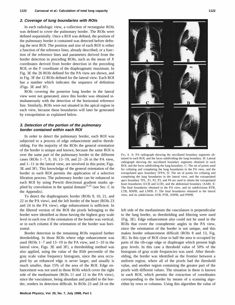
In each radiologic view, a collection of rectangular ROIswas defined to cover the pulmonary border. The ROIs weredefined sequentially. Once a ROI was defined, the position ofthe pulmonary border it contained was detected before defin-ing the next ROI. The position and size of each ROI is eithera function of the reference lines, already described, or a func-tion of the reference lines and parameters derived from theborder detection in preceding ROIs, such as the mean ofXcoordinates derived from border detection in the precedingROI, or theY coordinate of the diaphragmatic maximum. InFig. 3E the 26 ROIs defined for the PA view are shown, andin Fig. 3F the 12 ROIs defined for the lateral view. Each ROIhas a number which indicates the sequence of definition~Figs. 3E and 3F!.

ROIs covering the posterior lung border in the lateralview were not generated, since this border was obtained si-multaneously with the detection of the horizontal referenceline. Similarly, ROIs were not situated in the apical region ineach view, because these boundaries will later be generatedby extrapolation as explained below.

3. Detection of the portion of the pulmonaryborder contained within each ROI

In order to detect the pulmonary border, each ROI wassubjected to a process of edge enhancement and/or thresh-olding. For the majority of the ROIs the general orientationof the border is unique and known, because the same ROI isover the same part of the pulmonary border in the differentcases~ROIs 1–7, 9, 10, 13–19, and 21–26 in the PA view,and 1–11 in the lateral view, are involved in this point; Figs.3E and 3F!. This knowledge of the general orientation of theborder in each ROI permits the application of a selectivefiltration process. The pulmonary border can be enhanced ineach ROI by using Prewitt directional gradient masks ap-plied by convolution in the spatial domain21,22 ~see Sec. C inthe Appendix!.

To detect the diaphragmatic border~ROIs 9, 10, 21, and22 in the PA view!, and the left border of the heart~ROIs 23and 24 in the PA view!, edge enhancement is sufficient. Inthe filtered version of the ROI the pixels belonging to theborder were identified as those having the highest gray scalelevel in each row if the orientation of the border was vertical,or in each column if the orientation of the border was hori-zontal.

Border detection in the remaining ROIs required furtherthresholding. In those ROIs where edge enhancement wasused~ROIs 1–7 and 13–19 in the PA view, and 1–10 in thelateral view, Figs. 3E and 3F!, a thresholding method wasalso applied, using the value of the 85th percentile of thegray scale value frequency histogram, since the area occu-pied by an enhanced edge is never larger, and usually ismuch smaller, than 15% of the area of the ROI. Edge en-hancement was not used in those ROIs which cover the rightside of the mediastinum~ROIs 11 and 12 in the PA view!,since the vasculature, being abundant and parallel to the bor-der, renders its detection difficult. In ROIs 23 and 24 on the

left side of the mediastinum the vasculature is perpendicularto the lung border, so thresholding and filtering were used~Fig. 3E!. Edge enhancement also could not be used in theROIs that cover the costophrenic angles in the PA view,since the orientation of the border is not unique, and thismakes border enhancement difficult~ROIs 8 and 13, Fig.3E!. In this type of ROI close to half the area is occupied byparts of the rib-cage edge or diaphragm which present highgray levels. In this case a threshold value of 50% of thehistogram of gray scale frequencies was used. After thresh-olding, the border was identified as the frontier between auniform region, where all of the pixels had the thresholdvalue, and another region containing the greater part of thepixels with different values. The situation in these is knownin each ROI, which permits the extraction of coordinatescorresponding to the border by means of a scanning algo-rithm by rows or columns. Using this algorithm the value of

FIG. 4. A: PA radiograph showing the uncollated boundary segments ob-tained in each ROI, and the faces subdividing the lung boundary. B: Lateralradiograph showing the uncollated boundary segments obtained in eachROI, and the faces subdividing the lung boundary. C: The set of points usedfor collating and completing the lung boundaries in the PA view, and theextrapolated apex boundary TFPA. D: The set of points for collating andcompleting the lung boundaries in the lateral view, and the extrapolatedapex boundary TFL. P1, P2, P3, and P4 are used to obtain the extrapolatedheart boundaries~UCB and LCB!, and the abdominal boundary~AAB !. E:The final boundaries obtained in the PA view, and its subdivisions RTB,LTB, RNPB, and LNPB. F: The final boundaries obtained in the lateralview, and its subdivisions ATB, PTB, ANPB, and PNPB.

1122 Carrascal et al. : Calculation of total lung capacity 1122

Medical Physics, Vol. 25, No. 7, July 1998, Part 1

each pixel of a row or column is checked, beginning in theuniform area of the ROI with the threshold value, and ex-tracting the coordinates of the first pixel that has a valuedifferent from the threshold value in the row or column be-ing analyzed.

Before being used to define of the next ROI, all of thelung boundary segments detected as above are corrected byremoval of outlying pixels~which may correspond to bone,vasculature, or radiographic artifacts!. If the boundary seg-ment has a decidedly vertical or horizontal orientation, therange of boundary pixelX or Y coordinates is determined,and pixels with outlying coordinates are removed from theboundary set. If the boundary segment is not vertical or hori-zontal, the slopes of all pairs in the boundary set are calcu-lated, and points associated mostly with slopes lying outsidean appropriate range are removed from the boundary set.

4. Boundary completion and collation

The pulmonary borders need to be corrected in some partsand extrapolated in other parts, such as the apices and thecardiac border.

The segments of the pulmonary borders found in eachROI ~Figs. 4A and 4B! were completed and collated in threesteps. The first step consisted of filling in those portions ofthe border lacking pixels detected in each separate segment.The border was reconstructed on theY coordinate in verticalsegments, in such a way that it included the entire range ofYvalues between the maximum and minimum detected values.EachY coordinate was assigned its correspondingX coordi-nate from among those pertaining to the detection. In thecase of thoseY coordinates which for various reasons werenot among those detected, anX coordinate was assigned us-ing a linear interpolation between the points where these co-ordinates were missing. In the segments with a horizontalorientation, the border was reconstructed in the same way,but using theX coordinates, that is, assigning aY coordinateto everyX coordinate belonging to the range ofX coordi-nates of the segment.

The second step in the correction assured the continuitybetween the vertical segments and the horizontal diaphrag-matic segments in each view. In the apical regions, the pul-monary border was extrapolated by means of an arc whichconnected the vertical segments in both views. In the lateralview, the heart border and the anterior abdominal segmentwere extrapolated. The continuity between vertical segmentsand the horizontal segments was based upon the identifica-tion of the points of intersection of LDF with LLF and LMF,of RDF with RLF and RMF, and of DF with AF and PF,which are shown in Figs. 4C and 4D. If there existed a pixelof intersection, such as, for example, in the right costo-phrenic angle in Fig. 4A, the remaining points of the seg-ment were eliminated beyond this point. If it did not exist,each segment was extended by linear interpolation in thedirection determined by the final point and the point that layfive steps before, until the point of intersection was reached.

The third step is to determine the segments which corre-spond to the apical region in the PA view~TFPA! and in the

lateral~TFL! ~Fig. 4C!. TFPA is the result of the union of thehighest points of the LLF and RLF following a circular arcdefined by these two points and a third belonging to RLF,and placed 10% of the length of RLF below the highest RLFpoint. This circular arc is divided into three parts, with themiddle one truncated by replacing the circular part with ahorizontal line~Fig. 4C!.

TFL was obtained in a similar way by joining AF and PFby a circular arch defined by three points: the highest pointof PF, the highest point of AF, and a point of AF five stepsbefore the last one.

The definition of the borders of the heart in the lateralview was based on the automatic identification of four points~Fig. 4D!:

P1: intersection of AF and DF.P2: midpoint of a segment of the lower edge of the heart,

detected by means of the boundary enhancement and detec-tion procedures described above, in ROI 10 in lateral view.

P3: point near the hilum detected in ROI 11 in lateralview. An edge enhancement/detection procedure is applied;and, because the hilum region has the highest density ofenhanced edges, the point P3 is chosen at the center of thearea of highest detected edge density.

P4: point in the area of the intersection of AF and the topcardiac boundary detected in ROI 12 in lateral view. P4 isdefined by the same kind of thresholding-based procedure aswas used for defining the bottom horizontal reference lines~ACRREF and ACLREF! in the PA view.

Once P1, P2, P3, and P4 have been defined, they arejoined by two elliptical arcs belonging to ellipses withP1–P3 as major axes, one~UCB! passing through P1, P3,and P4 and the other~LCB! through P1, P3, and P2~Fig.4D!.

Finally, the anterior abdominal boundary in the lateralview ~AAB ! is defined as the perpendicular from P1 to thehorizontal line through the intersection of PF and DF~Fig.4D!. The fully constructed boundaries are shown in Figs. 4Eand 4F.

D. Determining total lung capacity

TLC may be calculated either by volumetric method ofellipses of Barnard’s method or by the planimetric Harrismethod. In the computer-aided implementation of Barnard’smethod, the elliptical cylindroids have a height of one pixel,a major axis that is the line joining the right and left lungedges in the PA view, and a minor axis which joins theanterior and posterior lung borders in the lateral view. Therelationship between the lung edges of the two views is ob-tained by aligning the coordinates of the pulmonary outlinefrom its apex. In Figs. 4E and 4F, the left and right lungedges are represented by LTB and RTB in the PA view, andthe anterior and posterior edges by ATB and PTB in thelateral. The computer calculation of the total thoracic volumeis carried out according to

TTV5( ~LTB i2RTBi !~PTBi2ATB i !PV CF,

1123 Carrascal et al. : Calculation of total lung capacity 1123

Medical Physics, Vol. 25, No. 7, July 1998, Part 1

where LTBi , RTBi , PTBi , and ATBi are theX coordinatesof the left, right, posterior, and anterior thoracic boundariesin the i th image lines of the corresponding views, PV is thepixel volume (0.08753 cm3), CF is the factorp/4 multipliedby (0.9)3 ~to correct for the 10% magnification of the radio-graphic image!, and the sum is taken over all image linesbetween the apex and the costophrenic angles.

TLC is determined by subtracting from TTV the volumesof tissue and blood and the volumes occupied by the heart,mediastinum, and subdiaphragmatic structures. The latter arealso considered elliptic cylindroids. The total lung capacity iscalculated by

TLC5TTV2NCV2BV2TV,

where BV ~blood volume! and TV ~pulmonary tissue vol-ume! are given by Lloydet al.:2

BV5244.122615.1358 hin10.035841 hin2,

TV52.73wp,

hin being the patient’s height in inches; wp being the pa-tient’s weight in pounds.

In Figs. 4E and 4F the edges of the nongas containingvolume structures~NCV! are shown as RNPB and LNPB inthe PA view and as ANPB and PNPB in the lateral. Thecomputer-aided calculation of the NCV follows:

NCV5( ~LNPBi2RNPBi !~PNPBi2ANPBi !PV CF,

where LNPBi , RNPBi , PNPBi , and ANPBi are theX coor-dinates in thei th image line of the corresponding view.

The planimetric method5,6 determines the TLC~in cm2!by the empirical formula

TLC58.53RLA21200,

whose computerized implementation is

RLA5AreaPA1AreaL,

AreaPA5( ~LTB i2RTBi !AP

2( ~LNPBi2RNPBi !AP,

AreaL5( ~PTBi2ATB i !AP

2( ~PNPBi2ANPBi !AP,

where AP is the pixel area (0.0875)2 cm2.

E. Evaluation of lung boundaries detection

To evaluate the precision of the automatically delineatedboundaries two methods were used:

The first one involved the subjective evaluation of threeexperienced radiologists, who rated independently the com-puter output over hard copies of the images using a five-point scale. A score of 5 was awarded if the boundaries were

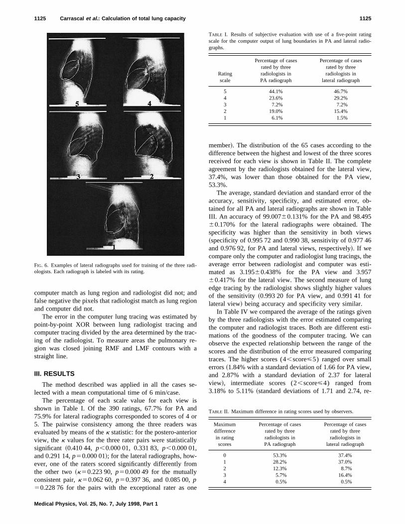
considered highly accurate, 4 if there was just one minorerror ~a moderate deviation affecting just a part of a singleboundary face!, 3 if there were two or more minor errors, 2 ifthere was a major error~a deviation affecting most of aboundary face!, and 1 if there were two or more major errors.The radiologists were trained in the use of the scale by beingshown three examples of radiographs of each rating value~Figs. 5 and 6 show one example for each value!. There wereno time constraints on rating the 65 pairs of test radiographs.

The second method was a comparison between the lungedges determined by the algorithm and those carefully tracedby one of the three radiologists with a mouse device. Tomeasure the accuracy, sensitivity and specificity, a pixel bypixel analysis procedure was used placing each pixel intoone of four categories: true positive~TP!, true negative~TN!,false positive~FP!, and false negative~FN!:14,23

sensitivity5TP/~TP1FN!,

specificity5TN/~TN1FP!,

accuracy5~TP1TN!/N,

whereN5number total of pixels. We consider: true positivethe pixels that computer and radiologist match as lung re-gion; true negative the pixels that computer and radiologistdid not match as lung region; false positive the pixels that

FIG. 5. Examples of PA radiographs used for training of the three radiolo-gists. Each radiograph is labeled with its rating.

1124 Carrascal et al. : Calculation of total lung capacity 1124

Medical Physics, Vol. 25, No. 7, July 1998, Part 1

computer match as lung region and radiologist did not; andfalse negative the pixels that radiologist match as lung regionand computer did not.

The error in the computer lung tracing was estimated bypoint-by-point XOR between lung radiologist tracing andcomputer tracing divided by the area determined by the trac-ing of the radiologist. To measure areas the pulmonary re-gion was closed joining RMF and LMF contours with astraight line.

III. RESULTS

The method described was applied in all the cases se-lected with a mean computational time of 6 min/case.

The percentage of each scale value for each view isshown in Table I. Of the 390 ratings, 67.7% for PA and75.9% for lateral radiographs corresponded to scores of 4 or5. The pairwise consistency among the three readers wasevaluated by means of thek statistic: for the postero-anteriorview, thek values for the three rater pairs were statisticallysignificant ~0.410 44, p,0.000 01, 0.331 83,p,0.000 01,and 0.291 14,p50.000 01!; for the lateral radiographs, how-ever, one of the raters scored significantly differently fromthe other two~k50.223 90,p50.000 49 for the mutuallyconsistent pair,k50.062 60,p50.397 36, and 0.085 00,p50.228 76 for the pairs with the exceptional rater as one

member!. The distribution of the 65 cases according to thedifference between the highest and lowest of the three scoresreceived for each view is shown in Table II. The completeagreement by the radiologists obtained for the lateral view,37.4%, was lower than those obtained for the PA view,53.3%.

The average, standard deviation and standard error of theaccuracy, sensitivity, specificity, and estimated error, ob-tained for all PA and lateral radiographs are shown in TableIII. An accuracy of 99.00760.131% for the PA and 98.49560.170% for the lateral radiographs were obtained. Thespecificity was higher than the sensitivity in both views~specificity of 0.995 72 and 0.990 38, sensitivity of 0.977 46and 0.976 92, for PA and lateral views, respectively!. If wecompare only the computer and radiologist lung tracings, theaverage error between radiologist and computer was esti-mated as 3.19560.438% for the PA view and 3.95760.417% for the lateral view. The second measure of lungedge tracing by the radiologist shows slightly higher valuesof the sensitivity~0.993 20 for PA view, and 0.991 41 forlateral view! being accuracy and specificity very similar.

In Table IV we compared the average of the ratings givenby the three radiologists with the error estimated comparingthe computer and radiologist traces. Both are different esti-mations of the goodness of the computer tracing. We canobserve the expected relationship between the range of thescores and the distribution of the error measured comparingtraces. The higher scores (4,score<5) ranged over smallerrors~1.84% with a standard deviation of 1.66 for PA view,and 2.87% with a standard deviation of 2.37 for lateralview!, intermediate scores (2,score<4) ranged from3.18% to 5.11%~standard deviations of 1.71 and 2.74, re-

FIG. 6. Examples of lateral radiographs used for training of the three radi-ologists. Each radiograph is labeled with its rating.

TABLE I. Results of subjective evaluation with use of a five-point ratingscale for the computer output of lung boundaries in PA and lateral radio-graphs.

Ratingscale

Percentage of casesrated by threeradiologists inPA radiograph

Percentage of casesrated by threeradiologists in

lateral radiograph

5 44.1% 46.7%4 23.6% 29.2%3 7.2% 7.2%2 19.0% 15.4%1 6.1% 1.5%

TABLE II. Maximum difference in rating scores used by observers.

Maximumdifferencein ratingscores

Percentage of casesrated by threeradiologists inPA radiograph

Percentage of casesrated by threeradiologists in

lateral radiograph

0 53.3% 37.4%1 28.2% 37.0%2 12.3% 8.7%3 5.7% 16.4%4 0.5% 0.5%

1125 Carrascal et al. : Calculation of total lung capacity 1125

Medical Physics, Vol. 25, No. 7, July 1998, Part 1

spectively! for the PA view, and from 3.93% to 5.92%~stan-dard deviations of 2.43 and 2.81, respectively! for the lateralview, and the lower scores (1<score<2) corresponded toerrors over 6.35% with standard deviation of 6.97 in the PAview ~in the lateral view the only value in this range did notgive significant results!.

The radiologists performed two manual measurements ofTLC by Barnhard’s method obtaining a good agreement. Theaverage of their differences was214.092 cm3 with a stan-dard deviation of 152.37 cm3 and a standard error18.894 cm3, Student’s T50.745 65, p50.229 31. Thismeans that the null hypothesis with 95% confidence cannotbe rejected, and thus there are not significant difference be-tween the averages of the measures. The automatic TLC cal-culation methods were evaluated by correlation of the com-puter measures with the two measures obtained by applyinga manual version of Barnhard’s method twice. Comparingthe average of the two TLC values obtained by manual Barn-

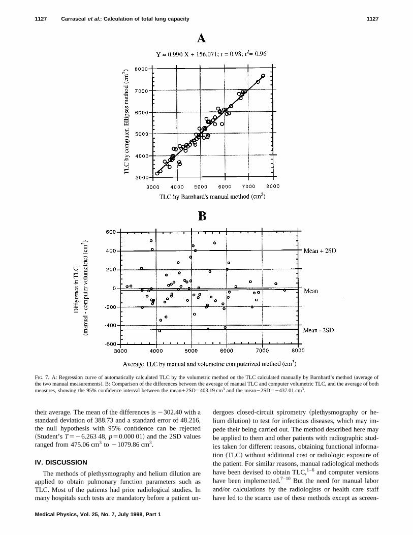
hard’s method with the computer implementation, a correla-tion coefficient of r 50.980 and a regression line ofY50.990X1156.071 are obtained. Figure 7 shows the scat-tergram comparing the average of manual TLC with thoseobtained automatically by the computer volumetric method,and the plot of differences between both TLC data againsttheir average. The mean of the differences is216.908 cm3

with a standard deviation~s.d.! of 210.05 cm3 and a standarderror of 26.054 cm3, the null hypothesis with 95% confi-dence can not be rejected~Student’s T50.648 95, p50.259 36! and the 2SD values ranged from 403.19 cm3 to2437.01 cm3. If we compare the computer implementationof the planimetric method on the manual Barnhard values, acorrelation coefficient ofr 50.933 and a regression line ofY50.771X11444.291 are obtained. Figure 8 shows the scat-tergrams comparing the manual TLC measures with thoseobtained automatically by the computer planimetric method,and the plot of differences between both TLC data against

TABLE III. Accuracy, sensitivity, specificity, and error calculated for PA and lateral views, comparing the lung boundaries traced by a radiologist with thosetraced by the computer and with a second trace by the same radiologist.

PA

Accuracy Sensitivity Specificity Error

Computertrace

2nd trace byradiologist

Computertrace

2nd trace byradiologist

Computertrace

2nd trace byradiologist

Computertrace

2nd trace byradiologist

Average 0.990 07 0.991 92 0.977 46 0.993 20 0.995 72 0.994 20 0.031 95 0.020 11

Standarddeviation

0.010 57 0.006 15 0.023 39 0.006 34 0.008 13 0.004 54 0.035 28 0.013 97

Standarderror

0.001 31 0.000 76 0.002 90 0.000 78 0.001 01 0.000 56 0.004 38 0.001 73

Lateral

Accuracy Sensitivity Specificity Error

Computertrace

2nd trace byradiologist

Computertrace

2nd trace byradiologist

Computertrace

2nd trace byradiologist

Computertrace

2nd trace byradiologist

Average 0.984 95 0.984 01 0.976 92 0.991 41 0.990 38 0.992 07 0.039 57 0.021 65

Standarddeviation

0.013 68 0.006 77 0.026 19 0.005 39 0.008 69 0.004 21 0.033 62 0.004 21

Standarderror

0.001 70 0.000 84 0.003 25 0.000 67 0.001 08 0.000 52 0.004 17 0.001 19

TABLE IV. Comparison between the average of the rating scores rated by the three radiologists and the errormeasured when radiologist and computer traces were compared.

PA

Averagescores

range:SNumberof cases

Averageerror

Standarddeviation

Standarderror

4,S<5 33 1.84% 1.66 0.293,S<4 15 3.18% 1.71 0.442,S<3 7 5.11% 2.74 1.041<S<2 10 6.35% 6.97 2.20

Lateral

Averagescores

range:SNumberof cases

Averageerror

Standarddeviation

Standarderror

4,S<5 31 2.87% 2.37 0.433,S<4 24 3.93% 2.43 0.492,S<3 9 5.92% 2.81 0.941<S<2 1 20.83% - -

1126 Carrascal et al. : Calculation of total lung capacity 1126

Medical Physics, Vol. 25, No. 7, July 1998, Part 1

their average. The mean of the differences is2302.40 with astandard deviation of 388.73 and a standard error of 48.216,the null hypothesis with 95% confidence can be rejected~Student’sT526.263 48,p50.000 01! and the 2SD valuesranged from 475.06 cm3 to 21079.86 cm3.

IV. DISCUSSION

The methods of plethysmography and helium dilution areapplied to obtain pulmonary function parameters such asTLC. Most of the patients had prior radiological studies. Inmany hospitals such tests are mandatory before a patient un-

dergoes closed-circuit spirometry~plethysmography or he-lium dilution! to test for infectious diseases, which may im-pede their being carried out. The method described here maybe applied to them and other patients with radiographic stud-ies taken for different reasons, obtaining functional informa-tion ~TLC! without additional cost or radiologic exposure ofthe patient. For similar reasons, manual radiological methodshave been devised to obtain TLC,1–6 and computer versionshave been implemented.7–10 But the need for manual laborand/or calculations by the radiologists or health care staffhave led to the scarce use of these methods except as screen-

FIG. 7. A: Regression curve of automatically calculated TLC by the volumetric method on the TLC calculated manually by Barnhard’s method~average ofthe two manual measurements!. B: Comparison of the differences between the average of manual TLC and computer volumetric TLC, and the average of bothmeasures, showing the 95% confidence interval between the mean12SD5403.19 cm3 and the mean22SD52437.01 cm3.

1127 Carrascal et al. : Calculation of total lung capacity 1127

Medical Physics, Vol. 25, No. 7, July 1998, Part 1

ing techniques.11,12 Paul et al. described an automaticmethod,10 but this was not used either. Our automaticmethod may be applied without any additional effort and isincreasingly favored in digital chest radiography. Additionalmedical appointments and the transporting of patients couldbe avoided thus saving time for both the patient and thehealth care personnel who carry out the plethysmograph orhelium dilution. Those hospitals not equipped with these sys-tems may use the information provided by TLC from asimple PA and lateral radiological study of the thorax.

Our method was only used on normal subjects. Its use in

abnormal subjects implies great CAD efforts in lung andthoracic disease. These studies are being developed in ourlaboratories and in other research centers. Detecting normal/abnormal lung vasculature,24 detection of nodules and pul-monary neoplasms, interstitial or pleural disease,25 compriseessential knowledge for testing TLC in abnormal patients.

The system requires two conditions to function properly.The first is the correct centering of the image. The patientshould not be rotated when this is obtained. Anatomic refer-ences allow us to precisely ascertain the correct centering ofthe radiologic exam, which in our study was verified in all

FIG. 8. A: Regression curve of automatically calculated TLC by the planimetric method on the TLC calculated manually by Barnhard’s method~average ofthe two manual measurements!. B: Comparison of the differences between the average of manual TLC and computer planimetric TLC, and the average of bothmeasures, showing the 95% confidence interval between the mean12SD5475.06 cm3 and the mean22SD521079.86 cm3.

1128 Carrascal et al. : Calculation of total lung capacity 1128

Medical Physics, Vol. 25, No. 7, July 1998, Part 1

cases. The second condition is that the radiological studymust be obtained at full inspiration. This requires the pa-tient’s collaboration. This limitation is also shared by pl-ethysmography and helium dilution.

Our method resembles the one devised by Paulet al. al-though with significant differences. The most significant dif-ferences involve the detection of the posterior and cardiacborders, and the determination of horizontal reference lines,and the size and localization of the ROIs which cover theedge, the arc designed to calculate the lung edge in the apex,and the directional gradient filter used for edge enhancement.

The edge enhancement and thresholding technique usedare sensitive to bone and vascular structures, artifacts, intes-tinal, or other type of gas, which may mask the lung edge. Inthese circumstances erroneous detection occurs of points out-side the lung edge. Most of these may be removed by algo-rithms for the elimination of outliers. This elimination ofpoints produces gaps in the detected edge, but the effect isminimized by the small size of the ROIs used and by theoverlap. Thus the extrapolation algorithms that eliminatethese gaps hardly introduce any errors in the outlining of thelung edges.

Enhancement and thresholding techniques were not ap-plied in apex regions in both views, and in the posteriorboundary and the boundary of the heart in the lateral view, asit produced a raised percentage of erroneous detection ofedges. The technique used in the posterior edge is less pre-cise in other regions due to its sensitivity to detection ofsmall relative maximum values, but in the posterior edge itprovides a higher level of approximation than the techniquesof edge enhancement and thresholding. The latter tend toenhance the vertebral edges more than the lungs in the regionof the posterior edge, whereas the technique used does notprovide detection of these edges, and produces a small num-ber of erroneous detection compared to the amount of pointsused to interpolate the lung edge. The use of extrapolation inthe edges of the apex and of the heart produced an overesti-mation or underestimation of the lung edge in some cases,which introduced a small error in the calculation of the lungvolume because they are regions of little content in volume.Less important errors observed in the lung outline occurredin more vascularized regions such as the mediastinum andhilum or were produced by the presence of intestinal gas inthe left hemidiaphragm.

The correlation coefficient obtained in our study betweenthe automatic method and Barnhard’s manual method, 0.980,is similar to the value 0.971 obtained by Paulet al.10 with asampling of 16 cases. The use of the Barnhard’s manualvolumetric method of as a standard with which to comparethe automatic method in calculating TLC, is justified by theproven high level of agreement between the results of themanual method and the direct measurement methods of TLCsuch as plethysmography2,3,6 and helium dilution.3 This levelof agreement is greater than in the planimetric method, asthis last is based in empirical formulas and overestimateslower values of TLC.6 As expected, the Barnhard automaticmethod is correlated better than with the manual method (r50.980) than with the planimetric method (r 50.933), dem-

onstrating a high level of agreement which is confirmed bythe absence of significant differences between the mean ofmanual measurements and the computer-assisted volumetricmethod~Student’sT50.648 95,p50.259 36, and the valuesof 2SD ranged from 403.192 cm3 to 2437.008 cm3!. Thecomputerized planimetric method has a low level of agree-ment with the mean of the manual measurements~Student’sT526.263 48,p50.000 01, and the value of 2SD rangedfrom 475.06 cm3 to 21079.86 cm3!.

The radiologists who took part in the study were givenprecise instructions. However, one of them showed a lowlevel of agreement with the findings of the other two, givinglower k statistical values in the PA view~0.331 83 and0.291 14!, and did not have a statistically significant level ofagreement in the lateral~0.062 60 and 0.085 00!. The highnumber of point values 4 and 5~67.7% for PA view, and75.9% for lateral view! leads us to believe that the discrep-ancies between the evaluators were due to different amountsof susceptibility to exaggerating the small errors. This notionis supported by the comparison of the average point scoreand the error measured when comparing the border drawn bythe computer with those carried out by the radiologist. As isshown in Table IV, the high point values (4,score<5)were errors of about 1.8% in the PA view, and of 2.8% in thelateral, with standard deviation of 1.66 and 2.37, respec-tively. These values are close to the intermediate values (2,score<4) which varied from 3.18%~standard deviation of1.71! to 5.11%~standard deviation of 2.74! in the PA view,and from 3.93%~standard deviation of 2.37! to 5.92%~stan-dard deviation of 2.81! in the lateral view.

To interpret the high values obtained for precision~0.990 07 for the PA view, and 0.984 95 for the lateral view!we should consider the high number of true negatives pixelspresent in the digital images. Duryea and Boone14 indicatethat precision does not provide a perfect indication of perfor-mance. Following on from their study, if all the pixels werenegatives or the positives were randomly distributed the pre-cision would provide high values~75%–79% and 63%–69%, respectively!, due to the high level of specificity~100%and 76.9%–82.4%, respectively!, while sensitivity is low~0% and 24.6%–17.9%, respectively!. In our case the sensi-tivity values~0.977 46 for the PA view, and 0.976 92 for thelateral view! and specificity~0.995 72 for the PA view, and0.990 38 for the lateral view! show that the latter possesses aslightly higher contribution to the precision values. If wecompare these values with those obtained in the second mea-surement carried out by the radiologist, precision~0.991 92for the PA view, and 0.984 01 for the lateral view! and speci-ficity ~0.994 20 for the PA view, and 0.992 07 for the lateralview! present similar values, but sensitivity is slightly higher~0.993 20 for the PA view, and 0.991 41 for the lateral view!,so the radiologist is slightly more precise than the computer.However, the difference is very small and we may considerthe level of approximation to the lung edge carried out by thecomputer is only slightly inferior to the border produced bythe radiologist.

We believe that the present work, which is readily appli-cable and low in cost, offers a good method for calculating

1129 Carrascal et al. : Calculation of total lung capacity 1129

Medical Physics, Vol. 25, No. 7, July 1998, Part 1

TLC in normal patients and adds functional information tothe conventional thoracic studies. The high precisionachieved in the automatic outline of the lung edges also al-lows it to be used in CAD systems, as demonstrated in pre-vious studies.13–18The increased use of digital thoracic radi-ology in hospitals26,27 will facilitate the implementation ofthis system in daily clinical practice.

ACKNOWLEDGMENTS

The authors are grateful to Kunio Doi, Ph.D., for his help-ful comments, and E. Lanz for editing the manuscript, bothfrom the Department of Radiology of the University of Chi-cago. They are also grateful to David Shea from the Univer-sity of Las Palmas de Gran Canaria for translating the manu-script. This study was supported in part by Grant No. 92/0487 of the Spanish Health Care Research Fund~Fondo deInvestigaciones Sanitarias de la Seguridad Social!.

APPENDIX: EXPLICIT ALGEBRAIC EXPRESSIONSFOR ALGORITHMS

A. Determination of vertical references RREF, LREF,AREF, and PREF

In the PA view successive profiles are examined startingat line 250 and working downward. In each profile ‘‘p’’ ( p<250) we defined: rref(p) first peak before right lung,lref(p) last peak after left lung, mref(p) right mediastinumand diaphragm boundaries. In each ‘‘p’’ the distance‘‘drm( p)’’ between rref and mref in each profile is obtainedas:

drm~p!5mref~p!2rref~p!,

when in a profile a value of drm(p),30 is reached the al-gorithm stops, obtaining the valuepr5p, used to define:

RREF5rref~pr !210; LREF5lref~pr !110. ~A1!

For the vertical reference lines of the lateral view, a simi-lar procedure is followed. In each horizontal profile ‘‘p’’ ofthe 10 lines at the middle of the image (239<p<248) wedefined: aref(p) first peak before the anterior lung boundary,pref(p) last peak after posterior lung boundary.

For each set of 10 peaks we obtained:

amean5mean$aref~p!%; asd5standard deviation$aref~p!%,

pmean5mean$pref~p!%; psd5standard deviation$pref~p!%,

arefmin5min$amean2asd<aref~p!%,

prefmax5max$pref~p!<pmean1psd%,

we defined:

AREF5arefmin220; PREF5prefmax120. ~A2!

B. Determination of horizontal references ACRREF,ACLREF, ACREF, and the posterior lungboundary

The horizontal reference lines at the bottom in the PAview are obtained in two ROIs that cover the diaphragm

areas in each lung~A and B!. Thresholding is applied overthe lung region contained in the ROIs at the 2/3 of the graylevel at the peaks in the ‘‘pr ’’ profile @the same as the usedin the Eq.~A1!#.

For ROI A the threshold level is tlA5rref ~pr !32/3.

For ROI B the threshold level is tlB5lref ~pr !32/3.

For each profile in each ROI, starting at the top

and working downward:

npA~p!5number of pixels with gray levels equal to

tlA in the profile p,

npB~p!5number of pixels with gray levels equal to

tlB in the profile p:

If npA~p!<5 then 1A5p.

If npB~p!<5 then 1B5p,

we defined:

ACRREF51A220; ACLREF51B220. ~A3!

Definition of the horizontal reference line in the lateralview is simultaneous to posterior lung boundary detection. Ineach horizontal profile ‘‘p’’ we defined a 100-pixel~a longi-tude of 100 pixels was chosen empirically! segment of inter-est ~SOI! as:

SOI~p!5~rf~p!, rf~p!1100!

where rf(p), that is, the lower extreme of the SOI(p), isdefined for each profile as:

for line p5250, rf~250!5PREF2100;

~Line 250 was chosen as start because is in the regionwhere the reference PREF is near to the posterior lungboundary!, for upper lines, a tentative lower extremerftent(p) is calculated as:

p.250, p5251,252,...

rftent~p!5rf~p21!2~PREF2max~p21!!

and for lower lines

p,250, p5249,248,...

rftent(p)5rf( p11)2(PREF2max(p11)), where max(p) isthe X coordinate of the first gray level peak detected inSOI(p) starting from right to left. max(p) is calculated as thesame form as lref.

rf( p) is then defined as

rf~p!5minimum of ~rftent~p!, PREF2100!.

In general, max(p) is the position~X coordinate! of theposterior lung boundary in linep, but below the costo-phrenic angle it occurs at a point somewhere near the centerof the abdomen. The definition of the horizontal referenceline in the lateral view is therefore based on examination ofthe differences:

1130 Carrascal et al. : Calculation of total lung capacity 1130

Medical Physics, Vol. 25, No. 7, July 1998, Part 1

ds~p!5max~p!2max~p11! ~A4!

for the profile p where ds(p) is maximum we definedpmax5p

ACREF5pmax. ~A5!

The provisional posterior boundary of the lung is the set ofpoints:$max(p),p% for p.ACREF.

C. Filtering employed

The boundary can be emphasized by use of a gradientdirectional mask by convolution in the spatial domain:

gi j 5 (k5 i 21

k5 i 11

(l 5 j 21

l 5 j 11

I kl mkl ~A6!

I : input image I kl : pixel value ofI in ~k,l ! coordinates

g: filtered image gi j :pixel value ofg in ~ i , j ! coordinates

m: gradient directional mask mkl :mask value in~k,l !

coordinates used ‘‘m’ ’ masks:

RIGHT LEFT TOP BOTTOM

F 21 1 1

21 22 1

21 1 1G F 1 1 21

1 22 21

1 1 21G F 1 1 1

1 22 1

21 21 21G F 21 21 21

1 22 1

1 1 1G

a!Correspondence: Francisco M. Carrascal, Departamento de Radiologı´a.Facultad de Medicina, San Francisco 1, 15704 Santiago de Compostela,Spain, Telephone: 34 81 570982, Fax: 34 81 547031, Electronic mail:mrpaco@correo.usc.es1H. J. Barnhard, J. Aa Pierce, J. W. Joyce, and J. M. Bates, ‘‘Roentgeno-graphic determination of total lung capacity. A new method evaluated inhealth, emphysema and congestive heart failure,’’ Am. J. Med.28, 51–60~1960!.

2H. M. Loyd, S. T. String, and A. B. Du Bois, ‘‘Radiographic and plethys-mographic determination of total lung capacity,’’ Radiology86, 7–14~1966!.

3T. M. Nicklaus, S. Watanabe, M. M. Mitchell, and A. D. Renzetti, Jr.,‘‘Roentgenologic, physiologic and structural estimations of the total lungcapacity in normal and emphysematous subjects,’’ Am. J. Med.42, 547–553 ~1967!.

4R. Greene, ‘‘Radiographic measurement of thoracic gas volume,’’ Rad.Clin. Nor. Amer.1, 63–71~1971!.

5P. C. Pratt and G. A. Klugh, ‘‘A method for the determination of totallung capacity from posteroanterior and lateral chest roentgenograms,’’Am. Rev. Resp. Dis.96, 548 ~1967!.

6T. R. Harris, P. C. Pratt, and K. H. Kilburn, ‘‘Total lung capacity mea-sured by roentgenograms,’’ Am. J. Med.50, 756–763~1971!.

7C. C. Jaffe, ‘‘A new technique for rapid determination of quantitative datafrom radiographs,’’ Radiology103, 451–453~1972!.

8P. G. Herman, T. Sandor, B. E. Man, E. R. McFadden, E. Korngold, M.A. Murphy, and H. Z. Mellins, ‘‘Rapid computerized lung volume deter-mination from chest roentgenograms,’’ Am. J. Roentgenol. Radium Ther.124, 477–483~1975!.

9W. W. Glenn and R. Greene, ‘‘Rapid computer-aided radiographic calcu-lation of total lung capacity,’’ Radiology117, 269–273~1971!.

10J. L. Paul, M. D. Levine, R. G. Fraser, and C. A. Laszlo, ‘‘The measure-ment of total lung capacity based on a computer analysis of anterior andlateral radiographic chest images,’’ IEEE Trans. Biomed. Eng.2, 444–451 ~1974!.

11R. O’Brien and T. Drizd, ‘‘Roentgenographic determination of total lungcapacity: normal values from a national population survey,’’ Am. Rev.Resp. Dis.128, 949–952~1983!.

12K. H. Kilburn, R. H. Warshaw, J. C. Thornton, and A. Miller, ‘‘Predictiveequations for total lung capacity and residual volume calculated fromradiographs in a random sample of the Michigan population,’’ Thorax47,519–523~1992!.

13M. F. McNitt-Gray, H. K. Huang, and J. W. Sayre, ‘‘Feature selection inthe pattern classification problem of digital chest radiograph segmenta-tion,’’ IEEE Trans. Med. Imaging14, 537–547~1995!.

14J. Duryea and J. M. Boone, ‘‘A fully automated algorithm for the seg-mentations of lung fields on digital chest radiographic images,’’ Med.Phys.22, 183–191~1995!.

15X-W. Xu and K. Doi, ‘‘Image feature analysis for computer-aided diag-nosis: Accurate determination of ribcage boundary in chest radiographs,’’Med. Phys.22, 617–626~1995!.

16G. F. Powell, K. Doi, and S. Katsuragawa, ‘‘Localization of inter-ribspaces for lung texture analysis and computer-aided diagnosis in digitalchest images,’’ Med. Phys.15, 581–587~1988!.

17N. Nakamori, K. Doi, V. Sabeti, and H. MacMahon, ‘‘Image featureanalysis and computer-aided diagnosis in digital radiography: Automatedanalysis of sizes of heart and lung in chest images,’’ Med. Phys.17,342–350~1990!.

18S. G. Armato, M. L. Giger, and H. MacMahon, ‘‘Computerized detectionof abnormal asymmetry in digital chest radiographs,’’ Med. Phys.21,1761–1768~1994!.

19E. D. Trout, J. P. Kelley, and V. L. Larson, ‘‘A comparison of an air gapand a grid in roentgenography of the chest,’’ Am. J. Roentgenol. RadiumTher.124, 404–411~1975!.

20H. S. Glacer, E. Muka, S. S. Sagel, and R. G. Jost, ‘‘New techniques inchest radiography,’’ Radiol. Clin. North. Amer.32, 711–729~1994!.

21R. Nevatia, Machine Perception, 1st ed. ~Prentice-Hall, EnglewoodCliffs, NJ, 1982!.

22E. R. Dougherty and C. R. Giardina,Matrix Structured Image Processing,1st ed.~Prentice-Hall, Englewood Cliffs, NJ, 1987!.

23C. E. Metz, ‘‘Basic principles of ROC analysis,’’ Seminars in NuclearMedicineVIII , 283–298~1978!.

24F. M. Carrascal, M. Cabrera, J. M. Carreira, L. Go´mez, and J. J. Vidal,‘‘Pulmonary vessels detection in digital chest radiographs applied to pul-monary vascular patterns recognition,’’ Proc. CAR , 368–373~1996!.

25K. Abe, K. Doi, H. MacMahon, M. L. Giger, H. Jia, X. Chen, A. Kano,and T. Wanagisawa, ‘‘Computer-aides diagnosis in chest radiography:preliminary experience,’’ Invest. Radiol.28, 987–993~1993!.

26C. R. Fuhrman, D. Gur, and R. Schaetzing, ‘‘High-resolution digital im-aging with storage phosphors,’’ J. Thorac. Imaging.5, 21–30~1990!.

27D. R. Aberle, D. Hansell, and H. K. Huang, ‘‘Current status of digitalviewal radiography of the chest,’’ J. Thorac. Imaging.5, 10–20~1990!.

1131 Carrascal et al. : Calculation of total lung capacity 1131

Medical Physics, Vol. 25, No. 7, July 1998, Part 1