automatic boosted flood mapping from satellite data...ing spectroradiometer (modis). modis is a...

January 19, 2016 International Journal of Remote Sensing floods

To appear in the International Journal of Remote SensingVol. 00, No. 00, Month 20XX, 1–22

Automatic Boosted Flood Mapping from Satellite Data

Brian Coltin∗, Scott McMichael, Trey Smith, and Terrence Fong

Intelligent Robotics Group, NASA Ames, Moffett Field, CA

(Received 00 Month 20XX; accepted 00 Month 20XX)

Numerous algorithms have been proposed to map floods from Moderate ResolutionImaging Spectroradiometer (MODIS) imagery. However, most require human input tosucceed, either to specify a threshold value or to manually annotate training data. Weintroduce a new algorithm based on Adaboost which effectively maps floods withoutany human input, allowing for a truly rapid and automatic response. The Adaboost al-gorithm combines multiple thresholds to achieve results comparable to state-of-the-artalgorithms which do require human input. We evaluate Adaboost, as well as numerouspreviously proposed flood mapping algorithms, on multiple MODIS flood images, aswell as on hundreds of non-flood MODIS lake images, demonstrating its effectivenessacross a wide variety of conditions.

Keywords: floods; flood mapping; MODIS; Adaboost

1. Introduction

Every year, floods claim an average of 140 lives and cause $6 billion in propertydamage in the United States alone (United States Geological Survey 2006). Withmaps of the flooded areas, produced rapidly and automatically from satelite oraerial imagery, responders can allocate their resources effectively to minimize lossof life and damage by quickly identifying the flooded areas (Taubenbock et al.2011).

Our ultimate goal, working with our partners at Google, is to deploy an onlinetool which will automatically and rapidly create and publish maps of floods. Thesemaps will be provided both to responders and to flood victims, complementingGoogle’s existing crisis response efforts.

The remote sensing community has already developed numerous algorithms andonline tools which rapidly map the extent of floods using multiple sources ofsatellite imagery. Existing online tools include the Dartmouth Flood Observatory(Brakenridge and Anderson 2006), the Global Flood Detection System (Kuglerand De Groeve 2007), and the Global Flood Monitoring System (Wu et al. 2014).However, these tools focus largely on the needs of researchers rather than the needsof flood responders and victims, as they are in a format not readily accessible orunderstandable by laypeople.

While preparing our own online flood mapping tool, we discovered that, despitesubstantial previous research in flood mapping algorithms, comparative, quanti-tative evaluation has been scant at best. Many algorithms have been introduced

∗Corresponding author. Email: [email protected]

1

https://ntrs.nasa.gov/search.jsp?R=20180002137 2020-07-28T21:32:51+00:00Z


for specific floods or regions, and their effectiveness has only been verified by sub-jective visual evaluation. Without quantitative evaluation, it is difficult to knowwhich algorithm to use in a given environment. To the best of our knowledge, onlyone quantitative evaluation of water detection algorithms has been done (Boschettiet al. 2014), but its focus was on flooded rice cropping systems, not floods. In ad-dition, the only algorithms evaluated were normalized difference spectral indicesthresholds. The lack of previous quantitative evaluations is largely due to threefactors:

(1) The challenge of establishing the ground truth flooding conditions with cer-tainty. Aside from taking physical measurements at the site of the flood, thereis no good way to establish the true flooding boundaries aside from evaluationof the geospatial imagery.

(2) The difficulty of acquiring imagery for multiple flood locations. Data sourceslike the Moderate Resolution Imaging Spectroradiometer (MODIS) andLandsat have large areas and times of coverage but are often occluded byclouds, while little SAR flood data is freely available. Furthermore, manyresearchers develop algorithms with the intent of studying only a single area.

(3) The computational challenges inherent in processing the imagery. Acquir-ing imagery is expensive in both time and bandwidth. Furthermore, exten-sive computational resources are required to process the imagery. However,processing images on a global scale is becoming more and more feasible ascomputational capabilities improve (Klein et al. 2015).

In this article we survey, compare and evaluate multiple flood mapping algo-rithms with the intent of choosing an algorithm for an online, fully automaticflood mapping tool. For challenge (1), establishing ground truth, we evaluate thealgorithms against our best-guess manually generated expert flood maps, as well asin hundreds of non-flood conditions using the permanent water mask. We addresschallenges (2) and (3) with the use of Google Earth Engine, an online platform forperforming massively parallel computation on geospatial imagery. Earth Enginesimplifies the research by pre-loading all of the imagery for common sources suchas MODIS and Landsat, and enabling simple and fast parallel processing of theimagery using Google’s servers. Earth Engine has enabled us to evaluate multiplealgorithms on hundreds of images. However, Earth Engine is limited to certaintypes of operations, mainly those which are easily parallelizable or local per pixelcomputations. Hence, our implementation of some algorithms differs slightly fromthe literature version, and we clearly note these changes. Our algorithms and dataare released as open source software so that future researchers can benefit from ourwork (available at https://github.com/nasa/CrisisMappingToolkit).

From the results of the evaluation, we realized that no existing algorithm succeedsin every scenario, and that the most successful existing algorithms require humaninput for tuning or training. For our intended fully automatic deployment, triggeredby online flood alerts, any human input is unacceptable. Hence, we propose the useof Adaboost for flood mapping. Adaboost combines multiple weaker classifiers tomake an algorithm that is much more robust to varying conditions than any oneclassifier on its own. The key insight which enables mapping without human inputis that non-flood conditions can effectively be used for training the weak classifiers.

We focus our flood mapping efforts on data from the Moderate Resolution Imag-ing Spectroradiometer (MODIS). MODIS is a sensor aboard the Terra and Aquasatelites which observes 36 spectral bands. MODIS observes the Earth’s entire sur-face every one to two days, making it effective for rapid flood mapping. However, it

2


cannot see through clouds and the bands are observed with low ground resolutionof 250 m/pixel or 500 m/pixel (Barnes, Pagano, and Salomonson 1998).

Several other data sources have also been used to map floods, including SynethicAperture Radar (SAR) (Martinis 2010; Matgen et al. 2011; Martinis, Twele, andVoigt 2009), microwave data from the Advanced Microwave Scanning Radiome-ter - Earth Observing System (ASMR-E) (Kugler, De Groeve, and Thierry 2007),precipitation estimates from the Tropical Rainfall Measuring Mission (TRMM)(Wu et al. 2014), and data from the Advanced Along-Track Scanning Radiometer(Fichtelmann and Borg 2012). Other researchers have also developed predictiveflood inundation maps in preparation for future flood events. For example, theGlobal Flood Awareness System predicts floods in advance using weather predic-tions and a hydrological model (Alfieri et al. 2013). The United States GeologicalSurvey (USGS) creates libraries of inundation maps for numerous locations whichdescribe the expected flood extent given the readings on nearby USGS streamgauges (United States Geological Survey 2015). Furthermore, remote sensing ofwater is useful not only for the formation of wet / dry maps, but also to develophydraulic models to better understand and mitigate flood damage (Schumann et al.2009).

In the remainder of this article, we first present existing flood mapping algorithmsfor MODIS data. Next, we introduce our Adaboost algorithm, which effectively andfully automatically classifies floods. Finally, we present an extensive evaluation ofthe effectiveness of our approach on a small number of floods and on hundreds oflakes.

2. Review of MODIS Flood Mapping Algorithms

The two MODIS satellites, Terra and Aqua, achieve global coverage every oneto two days which makes them suitable for rapid response flood mapping. Theymeasure 36 spectral bands. We denote the surface reflectance from MODIS band ias Bi. The wavelengths measured by the MODIS bands are: B1, 620-670 nm; B2,841-876 nm; B3, 459-479 nm; B4, 545-565 nm; B5, 1230-1250 nm; B6, 1628-1652nm; and B7, 2105-2155 nm. The remaining bands are unused in this work. B1

and B2 have a 250m resolution, B3–B7 have a 500m resolution, and the remainingbands have a 1000m resolution (Barnes, Pagano, and Salomonson 1998). This lowresolution may not be sufficient to determine if individual homes are flooded, butis useful in directing large scale response efforts.

Another drawback of MODIS is that it is often occluded by clouds. Numerouscloud detection algorithms have been developed for MODIS (Frey et al. 2008),and it is possible to filter clouds before applying any flood detection algorithms.However, to better focus our evaluation on flood detection algorithms, we evaluatedcloud-free MODIS scenes only and set aside the challenge of cloud filtering.

We first review a number of algorithms from the literature for flood mapping withMODIS, which we later evaluate using Google Earth Engine. Our evaluation is notexhaustive, and some notable omissions include transforming MODIS images tothe Hue Saturation Value (HSV) color space for flood detection (Pekel et al. 2014)and dynamic thresholding based on tiling (Klein et al. 2015).

3


Table 1. Table of MODIS indices.

Index Equation

Normalized Difference Water Index (NDWI) B1−B6B1+B6

Land Surface Water Index (LSWI) B2−B6B2+B6

Normalized Difference Vegetation Index (NDVI) B2−B1B2+B1

Enhanced Vegetation Index (EVI)2.5(B2−B1)

6B1+B2−7.5B3+1

2.1. Thresholding Algorithms

One of the simplest and most common flood mapping algorithms for MODIS datais to apply thresholds to one or more indices computed from the higher resolutionMODIS bands. These thresholding algorithms can achieve good results, are com-putationally inexpensive, and are easily implemented. However, they must oftenbe calibrated for a specific region or dataset, as the most discriminating thresh-olds are highly dependent on both the water content and the surrounding land’sspectral properties. This need for human input to select a threshold precludes fullyautomatic deployment.

2.1.1. Islam

The Islam algorithm thresholds an image based on the Enhanced Vegetation Index(EV I) and Land Surface Water Index (LSWI) (see Table 1 for definitions ofMODIS indices). Pixels which satisfy the formula

((EVI) ≤ 0.3 ∧ (EVI)− (LSWI) ≤ 0.05) ∨ ((EVI) ≤ 0.05 ∧ (LSWI) ≤ 0.0) (1)

are marked as water (where ∧ indicates logical and, and ∨ is logical or). Theoriginal algorithm further segments these pixels into flooded, partially flooded,and permanent water bodies (Islam, Bala, and Haque 2009). The Islam algorithmdoes not contain any adjustable thresholds, and was originally developed solely fora flood in Bangladesh; thus, it was uncertain how and if it would generalize tofloods in other regions. This does give it the advantage of being fully automatic,not requiring any human intervention.

2.1.2. Xiao

A similar approach used to detect floods is the Xiao algorithm. Pixels which satisfythe formula

((LSWI)− (EVI) ≥ 0.05) ∨ (2(LSWI)− (NDVI) ≥ 0.05) (2)

are marked as flooded. This approach, together with a further filtering step, wasoriginally designed to detect rice paddies and was successfully applied in southeastAsia (Xiao et al. 2006). Like Islam, the Xiao algorithm has the advantage of beinghuman input-free.

2.1.3. Diff

The Diff algorithm classifies pixels which satisfy the formula

B2 −B1 ≤ KDiff (3)

4


as flooded. The threshold KDiff is a parameter that is chosen for each region basedon the properties of the water and surrounding land areas. This simple algorithmis surprisingly effective. However, it requires a human to specify the thresholdmanually.

2.1.4. Dart

The Dartmouth flood observatory maps worldwide surface water with MODIS us-ing a cloud filter together with a thresholding algorithm (Brakenridge and Anderson2006). The Dart algorithm classifies pixels which satisfy the equation

B2 + C

B1 +D≤ KDart (4)

as flooded. This algorithm requires three constants to be specified, C, D, andKDart, all of which are determined empirically (Brakenridge 2012).

2.1.5. Mndwi

The study by Boschetti et al. (2014) compares a large number of normalized dif-ference spectral indices (indices in the form A−B

A+B ) and evaluates them on a fewregions of rice crops. One of the most effective indices in this study was the Modi-fied Normalized Difference Water Index:

B6 −B4

B6 +B4≤ KMndwi. (5)

We evaluate the Mndwi as representative of normalized difference spectral indices.The constant KMndwi must be manually specified for each problem instance.

2.1.6. Fai

The Floating Algae Index (Fai) classifies pixels where

B2 −(B1 +

859− 645

1240− 645(B5 −B1)

)≤ KFai (6)

as flooded. The Fai is promising for separating land and water because it is believedto be less sensitive than other indices to local environmental conditions (Feng et al.2012). The constant KFai must be manually specified for each problem instance.

2.1.7. Theme

The Thematic MODIS Processor (Theme) is a decision tree using EVI/LSWIthresholds, slope measurements, and region growing steps to classify pixels into oneof six flood-related output classes. It is the most complicated of the thresholdingapproaches we considered; for a full description see Martinis et al. (2013).

First, Theme begins with the water classification from the Islam algorithm.Then, flooded pixels on which the DEM shows a high slope are marked as un-flooded. Finally, a region growing step marks pixels neighboring flooded pixels asflooded if they satisfy a looser version of the Islam thresholding constraints. Notethat due to Earth Engine limitations, we approximate the region growing step.

5


2.2. Supervised Learning

The next class of algorithms we consider are supervised learning approaches. Wherethe thresholding approaches require a human operator to provide at most a singlethreshold value, supervised learning approaches require training data in the form ofan annotated flood region. The algorithm uses this region to learn how to identifyfloods in additional data. For supervised learning algorithms to be successful thetraining data must be similar to the test data.

Supervised learning algorithms are expected to outperform the other algorithms(depending on the quality of the training data) as they have more data to work withand draw conclusions from, but the requirement of human-produced training datarenders them less promising for rapid response. It is possible that with enough data,a general classifier could be learned for any flood. Unfortunately, due to the rarityof flood events and the huge variation among ground conditions this is challenging.

A number of features have previously been suggested for supervised flood map-ping: B1, B2, B2−B1, B2

B1, the NDWI, and the NDVI (Sun, Yu, and Goldberg 2011).

Using these features, we consider three different supervised learning approaches:

• Cart: A classification and regression tree (Olshen and Stone 1984) formsa tree of rules by which to classify flooded and unflooded pixels. Cart waspreviously proposed for use in flood mapping (Sun, Yu, and Goldberg 2011).• Rf: The Random Forests algorithm constructs an ensemble of decision trees

which then vote on whether a pixel is flooded (Breiman 2001). Rf was pre-viously proposed for use in flood mapping (Sun, Yu, and Goldberg 2011).• Svm: The final supervised learning approach is a support vector machine

solved with the Pegasos solver (Shalev-Shwartz et al. 2011). While to ourknowledge it has not previously been used for flood mapping, it is a popularmachine learning algorithm.

2.3. Dynamic Nearest Neighbor Searching

The previous thresholding and supervised learning approaches (with the exceptionof Theme) all operate on the level of individual pixels, and do not take any contex-tual information into account. However, the surrounding pixels are an importantsource of additional information. Intuitively, when humans solve the flood map-ping problem, they are completely unable to determine whether individual pixelsin isolation are flooded. It is only when presented with groups of pixels that pat-terns emerge and humans are able to identify flooding. The two Dynamic NearestNeighbor Searching (DNNS) algorithms rely heavily on measurements of nearbylocations to classify each pixel.

2.3.1. Dnns

Dnns incorporates contextual information. As with the supervised learning algo-rithms, training data is required.

The Dnns algorithm (Li et al. 2013b) is shown in Algorithm 1. First, “pure wa-ter” and “pure land” pixels are determined from a variant of the Rf classifier whichoutputs “mixed” pixels as well. Then, for each pixel in the image, Dnns averagesthe surrounding pixels detected as pure water to compute an estimated regionalwater reflectance. From this pure water reflectance, the neighboring land pixels aredetermined, and an average land reflectance is estimated. From the average waterand land reflectance and the MODIS B6 value, a “water fraction”, or how much

6


function Dnns(B)

Wpure ← PureWater(B),Lpure ← PureLand(B)

for (i, j) ∈ B do

N←{

(i′, j′) :√

(i− i′)2 + (j − j′)2 ≤ RD

}. Neighboring Pixels

Wmean ← 1|N∩Wpure|

∑(i′,j′)∈N∩Wpure

B(i′, j′) . Mean Water Reflectance

Nland ←

{(i′, j′) ∈ N :

B1(i,j)−Wmean,1

B6(i,j) < B1(i′,j′)B6(i′,j′) <

B1(i,j)B6(i,j) ,

B2(i,j)−Wmean,2

B6(i,j) < B2(i′,j′)B6(i′,j′) <

B2(i,j)B6(i,j)

}Lmean ← 1

|Nland|∑

(i′,j′)∈NlandB(i′, j′) . Mean Land Reflectance

Wf(i, j)←

0 if (i, j) ∈Wpure

1 if (i, j) ∈ LpureLmean,6−B6(i,j)Lmean,6−Wmean,6

otherwise

. Water Fraction

end for

return Wf

end function

Algorithm 1: The Dynamic Nearest Neighbor Searching flood mapping algo-

rithm (Li et al. 2013b). B is the multi-band MODIS image, (i, j) ∈ B are the

pixel coordinates. Edge cases where |N ∩Wpure| = 0, |Nland| = 0 are omitted.

of the pixel contains water, is estimated. The water fraction is only applied to themixed pixels.

2.3.2. Ddem

The DNNS with Digital Elevation Maps (DEMs) algorithm, Ddem, improves onDnns by modifying the result based on a DEM (Li et al. 2013a). While MODIShas 500m and 250m pixels, the worldwide SRTM 90m DEM (Farr et al. 2007) andthe United States’ National Elevation Dataset 10m DEM (for the 48 continentalUS states only) (Gesch et al. 2002) are much higher resolution, allowing the con-struction of a more detailed flood map. However, this detail does not come fromempirical observation, but from modelling of the flow of water based on the terrainmodel.Ddem uses the water fraction from Dnns for each MODIS pixel and a histogram

of the DEM elevations in the MODIS pixel to select the flood level consistent withthe observed values. Then, since water levels are flat, a filtering step smooths theelevations of connected water bodies. The key idea is that the partially floodedpixels offer the most information about the water level. See Algorithm 2 for theApplyDem algorithm, which takes the water fraction output from Dnns as input.

3. Fully Automatic Flood Mapping

Of the MODIS algorithms we reviewed, only Evi, Xiao, and Theme are fully au-tomatic, requiring no human input. The other algorithms either require humans tospecify a threshold value or provided annotated training data, making them un-suitable for rapid, fully automatic response. Furthermore, existing fully automaticalgorithms fare poorly across different regions (as we will show in our experimentalresults). Hence, we introduce several algorithms which are more robust to differing

7


function ApplyDem(Wf, D)

H,O← Empty Images

for (i, j) ∈Wf do

Wmin ← minDEM pixels (x,y) in Wf(i,j)D(x, y)

Wmax ← maxDEM pixels (x,y) in Wf(i,j)D(x, y)

H(i, j)←Wmin + Wf(i, j) (Wmax −Wmin) . Estimate Water Height

end for

for (i, j) ∈Wf do

Wnum ←{

(i′, j′) : 0 < Wf(i′, j′) < 1 ∧

√(i− i′)2 + (j − j′)2 ≤ RM

}Hmean ← 1

|Wnum|∑

(i′,j′)∈WnumH(i′, j′) . Average Region Water Height

for DEM pixels (x, y) ∈Wf(i, j) do

O(x, y)← D(x, y) < Hmean . Fill DEM Under Water

end for

end for

return O

end function

Algorithm 2: The ApplyDem algorithm, which produces a flood map from a water

fraction Wf and a DEM D. RM is a constant, the radius within which to aver-

age water heights. Note that our water height estimation differs from the original

algorithm (see Section 4.1.2).

0.0

0.2

0.4

0.6

0.8

1.0

-500 0 500 1000 1500 2000 2500 3000 3500

Prec

isio

n / R

ecal

l

KDiff

PrecisionRecall

(a)

0.0

0.2

0.4

0.6

0.8

1.0

-500 0 500 1000 1500 2000 2500 3000 3500

Prec

isio

n / R

ecal

l

KDiff

PrecisionRecall

(b)

Figure 1. Precision and recall curves for the Diff algorithm as a function of KDiff, evaluated on the (a)

New Orleans and (b) Kashmore floods.

ground conditions and require no human input.

3.1. Learning Thresholds Automatically

The Diff, Dart, Fai, and Mndwi algorithms perform reasonably well across avariety of flood conditions, but require a single threshold value to be specifiedmanually. The threshold which achieves the best point on the precision / recallcurve varies between domains, and depends on both the appearance of the waterand the surrounding land (Fichtelmann and Borg 2012; Klein et al. 2015). Forexample, Figure 1 shows how differently the same thresholds for the Diff methodperform on a flood in Louisiana and a flood in Kashmore.

To eliminate the need for manual human intervention, we introduce an algorithmthat computes these thresholds automatically. The key idea is that although the

8


flood conditions vary widely from non-flood conditions, non-flood conditions maystill be suitable for estimating a good threshold value, even if that threshold is notperfectly adjusted for the flood conditions.

We search for a MODIS image of the same area from one year before the testdate without clouds. If such an image is not available the search is extended toprevious years. We choose an image from the same time of year in order to obtaintraining data with similar seasonal land cover.

Histograms of the water and land pixel values are generated from the historicalimage, with the 250m MOD44W permanent water mask (Carroll et al. 2009) usedas ground truth. Let WT and LT be the sets of water and land pixels as thresholdedby a threshold T , and W and L be the true sets of water and land pixels accordingto the permanent water mask. We choose the threshold T that maximizes

|LT ∩ L||L|

|WT ∩W||W|

(7)

where |A| is the size of set A in order to minimize mislabelings for both classes.We then evaluate the original test image with the threshold T .

This automatic approach for learning thresholds is applied to the MODIS thresh-olding algorithms Diff, Dart, Mndwi, and Fai in order to create the DiffL,DartL, MndwiL, and FaiL algorithms. These approaches require no human in-put, but since water in the flood image may have a different appearance than thewater in the historical image, they do not select as good of a threshold as a humanwould.

3.2. Combining Thresholds with Adaboost

The automatically learned thresholds require no human supervision. However, thereis no uniformly “best” thresholding algorithm. Each performs well in certain situ-ations and poorly in others.

To address the shortcomings of the individual thresholds, we propose an al-gorithm based on Adaboost (Freund and Schapire 1997) that combines multiplethreshold-based classifiers into a single more effective classifier, which is robust andworks well across a diverse range of flood scenarios. Like the automatically learnedthresholding approaches, this algorithm can be trained on on limited historicaldata, and does not need to be trained post-flood. In fact, the algorithm is effectiveeven if it has not been trained on a particular location.

The algorithm Ada is shown in Algorithm 3. Ada requires a set of indices Ii(which are functions of MODIS bands), thresholds for these indices Ki, and weightsfor each individual classifier αi. Each individual classifier may not be very accurate,but when added together and weighted the classifiers achieve a high precision andrecall.Ada returns an image of real numbers, such that positive pixels are flooded and

negative pixels are dry. However, we have found that the classification favors falsenegatives over false positives. We shift along the precision / recall curve in favorof recall by thresholding the output of Ada by -1, such that pixels with a valueover -1 are marked as flooded. See Figure 2 for an example of this precision recallcurve.

The indices, thresholds and their weights are learned with the procedure Lear-nAda shown in Algorithm 4. The LearnAda procedure learns from multiple floodimages at once. It learns up to M weak classifiers. (We use M = 50, terminating

9


function Ada(B, I , K , α)

R← 0

for i = 1..N do

C← image s.t. C(i, j) =

{1 if I i(B)(i, j) ≤ Ki

−1 otherwise

R← R+ αiC

end for

return R

end function

Algorithm 3: The Ada algorithm, which produces a flood map from a MODIS

image B, and lists of N MODIS indices I i, thresholds K i, and weights αi. In the

returned image, positive pixel values are classified as flooded pixels.

0.0

0.2

0.4

0.6

0.8

1.0

0.0 0.2 0.4 0.6 0.8 1.0

Recall

Precision

Figure 2. An example precision / recall curve for an image of a flood on the Mississippi in June 2011 (seeSection 4.1 for details on the evaluation image).

early if a cycle is reached, but note that each additional classifier is subject to dimin-ishing returns, and overfitting is possible.) Each iteration, a new weak classifier ischosen with the lowest weighted error based on a matrix W of pixel weightings. Weiterate over all possible index functions, and search for thresholds halfway betweenpreviously used thresholds. We initiate the list of previous threshold choices withthe 20th and 80th percentiles of the flooded pixels in the training data, boundingthe searched thresholds to this range.

Once a weak classifier (both index function and threshold) is chosen, a weight αfor that classifier is computed. The weights of the image pixels in W are then up-dated, such that pixels the selected weak classifier incorrectly classifies are weightedmore heavily in the future. Thus, LearnAda focuses on pixels it previously failedon when learning new classifiers. After M weak classifiers are identified, a list ofthe classification functions, the selected thresholds, and the classifier weights α isgenerated. These lists are then used by Ada to map floods.

For MODIS data, we learn from the following index functions:

10


function LearnAda(B, T)

Iall ← All considered index functions

for f ∈ Iall do

a, b← 20th, 80th percentile in histogram of f(B) s.t. T

s f ← [a, b, b+ (b− a)] . List of previously chosen thresholds.

end for

I = [] ,K = [] , α = []

W = 1|B| . Matrix of weights for all pixels in B, begin normalized

for i = 1..M do

. Choose classifier and threshold to minimize weighted error

(f, j)← arg minf∈I all,0≤j<|sf|−1 ε = W · ((f(B) ≤ sf,j+sf,j+1

2 ) 6= T)

K ← sf,j+sf,j+1

2

αi ← 12 ln 1−ε

ε

∀x, y D(x, y)←

{1 if f(B)(x, y) ≤ K−1 otherwise

W← e−αiDW . Update weights

W←W/∑

x,y W(x, y) . Normalize weights

Append f, k, αi to I ,K , α.

end for

return I ,K , α

end function

Algorithm 4: This algorithm learns the weak classifiers and weights for use in

Ada. B is a union of potentially multiple input MODIS images, and T is a ground

truth mask indicating which pixels are flooded (0 is dry, 1 is flooded). Operations

on images are performed individually on every pixel of the image. Comparison

operators on images return 0 for false and 1 for true on a per-pixel basis, and

M ·N is element-wise multiplication.

• B1

• B2

• B2/B1

• EVI• LSWI

• NDVI• NDWI• LSWI - NDVI• LSWI - EVI• Diff

• Dart• Fai• Mndwi

Ada uses combinations of all these features for classification. Where a thresholdingalgorithm is specified, we use the intermediate result in the algorithm that thethreshold is applied to.

If further algorithms are developed which output a continuous range of values,Ada can also incorporate them as training features. Ada’s inputs do not even needto be from MODIS. In fact, we have successfully incorporated SAR and Landsatdata into Ada, by simply adding the additional information as index functions.Then Ada automatically learns which satellites and index functions to incorporateinto the classifier. Figure 3 shows an example of Ada and the results of thresholdingtwo of its inputs.

11


(a) (b) (c)

(d) (e) (f)

Figure 3. The results of several different flood mapping algorithms applied to a flood of the Mississippi.

Ada combines multiple approaches and is more robust than individual algorithms. (a) Landsat overlaid

with ground truth annotation. (b) Dart. (c) Theme. (d) Ada unthresholded output. (e) Ada. (f) AdaDem.The horizontal artifacts are caused by artifacts in the DEM. All images are from Landsat 5, path 27 row

37, taken on 10 Oct. 2011 with a top left corner at 33.16◦N, 91.24◦W.

3.3. Fine-tuning Adaboost with the DEM

The output of Ada is at MODIS’ 250m resolution. However, as with DNNS, wecan perform mapping at a higher resolution by incorporating the DEM. In fact, wecan apply the exact same ApplyDem algorithm as Ddem uses. We merely shiftthe output of Ada, adding one to the output and clamping between 0 and 1, andpass that image as the water fraction to ApplyDem. This means that pixels with avalue less than −1 (our looser threshold used to adjust the results in favor of recall)in the image from Ada will be considered land, and pixels with a value greaterthan 0 (the original threshold) are considered water. It is unclear if the assumptionbehind Dnns, that a pixel with water fraction 0.7 has 70% of its surface areacovered with water, holds for this case. Figure 3 shows an example of Ada andAdaDem.

12


4. Experimental Evaluation and Discussion

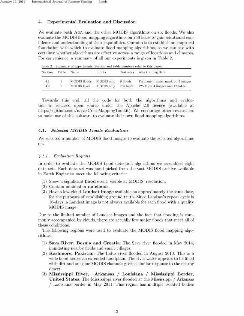
We evaluate both Ada and the other MODIS algorithms on six floods. We alsoevaluate the MODIS flood mapping algorithms on 756 lakes to gain additional con-fidence and understanding of their capabilities. Our aim is to establish an empiricalfoundation with which to evaluate flood mapping algorithms, so we can say withcertainty whether algorithms are effective across a range of locations and climates.For convenience, a summary of all our experiments is given in Table 2.

Table 2. Summary of experiments. Section and table numbers refer to this paper.

Section Table Name Inputs Test sites Ada training data

4.1 4 MODIS floods MODIS only 6 floods Permanent water mask on 5 images

4.2 5 MODIS lakes MODIS only 756 lakes PWM on 4 images and 12 lakes

Towards this end, all the code for both the algorithms and evalua-tion is released open source under the Apache 2.0 license (available athttps://github.com/nasa/CrisisMappingToolkit). We encourage other researchersto make use of this software to evaluate their own flood mapping algorithms.

4.1. Selected MODIS Floods Evaluation

We selected a number of MODIS flood images to evaluate the selected algorithmson.

4.1.1. Evaluation Regions

In order to evaluate the MODIS flood detection algorithms we assembled eightdata sets. Each data set was hand picked from the vast MODIS archive availablein Earth Engine to meet the following criteria:

(1) Show a significant flood event, visible at MODIS’ resolution.(2) Contain minimal or no clouds.(3) Have a low-cloud Landsat image available on approximately the same date,

for the purposes of establishing ground truth. Since Landsat’s repeat cycle is16-days, a Landsat image is not always available for each flood with a qualityMODIS image.

Due to the limited number of Landsat images and the fact that flooding is com-monly accompanied by clouds, there are actually few major floods that meet all ofthese conditions.

The following regions were used to evaluate the MODIS flood mapping algo-rithms:

(1) Sava River, Bosnia and Croatia: The Sava river flooded in May 2014,inundating nearby fields and small villages.

(2) Kashmore, Pakistan: The Indus river flooded in August 2010. This is awide flood across an extended floodplain. The river water appears to be filledwith dirt and on some MODIS channels gives a similar response to the nearbydesert.

(3) Mississippi River, Arkansas / Louisiana / Mississippi Border,United States: The Mississippi river flooded at the Mississippi / Arkansas/ Louisiana border in May 2011. This region has multiple isolated bodies

13


of water and substantial vegetation, making it one of the most challengingregions we address. Due to the vegetative cover this region has considerableuncertainty in the human generated ground truth map.

(4) Mississippi River, Arkansas / Louisiana / Mississippi Border,United States: This covers the same region as the previous flood, but amonth later when the water level has risen even further. The appearance ofthe nearby fields has changed considerably as the crops have grown.

(5) Katrina, New Orleans, United States: The city of New Orleans wasflooded after Hurricane Katrina. This is a densely populated urban area.The flood is difficult to see from Landsat imagery, so maps generated fromon-the-ground observations were used to construct the ground truth map.

(6) Assiniboine River, Manitoba, Canada: Significant precipitation causedthe Assiniboine River to flood in Manitoba. The test area is near the town ofSt. Lazare. This domain is especially challenging since the river is quite nar-row compared to the MODIS resolution, and nearby fields appear as flooded.

(7) Parana River, Argentina: The Parana river flooded due to heavy rainfall.The flood region is located near the border with Paraguay, and includes thetown of Corrientes.

(8) Shire River, Malawi: Malawi suffered a devastating flood in January 2015.The Shire River dramatically exceeded its usual boundaries but the floodwater is is broken up by small outcroppings of land. High resolution SkyboxRGB imagery aided in generating the ground truth for this region.

Table 3. Test domain details.

MODIS Ground Truth Coordinates of Bounding box

ID Name Date Date Satellite Bottom left Top right

1 Sava 21 May 2014 22 May 2014 Landsat 8 44.919◦N, 18.507◦E 45.101◦N, 18.809◦E

2 Kashmore 13 Aug. 2010 12 Aug. 2010 Landsat 5 28.250◦N, 69.500◦E 28.650◦N, 70.100◦E

3 Mississippi 8 May 2011 10 May 2011 Landsat 5 32.880◦N, 91.230◦W 33.166◦N, 91.020◦W

4 Mississippi 12 June 2011 11 June 2011 Landsat 5 32.880◦N, 91.230◦W 33.166◦N, 91.020◦W

5 Katrina 7 Sep. 2005 7 Sep. 2005 Landsat 5 29.900◦N, 90.300◦W 30.070◦N, 89.760◦W

6 Assiniboine 1 June 2011 1 June 2011 Landsat 5 50.200◦N, 101.690◦W 50.460◦N, 101.330◦W

7 Parana 19 July 2014 19 July 2014 Landsat 8 27.750◦S, 58.950◦W 27.500◦S, 58.750◦W

8 Malawi 21 Jan. 2015 21 Jan. 2015 Skybox 17.090◦S, 35.180◦E 16.870◦S, 35.320◦E

The exact bounding boxes and the sources of the MODIS and ground truth im-ages are listed in Table 3. Partial images of the test areas are shown in Figure 4. Ouraim was to select a wide range of flood conditions, representative of the diversityof floods worldwide.

4.1.2. Methodology

For each domain, we evaluate each algorithm numerically against a “ground truth”image by computing the precision P and recall R for the flooded regions. Let T bethe set of pixels flooded in the ground truth image, and G be the set of pixels thealgorithm guesses are flooded. Then

P =|T ∩G||G|

, R =|T ∩G||T|

. (8)

14


(a) (b) (c)

(d) (e) (f)

Figure 4. Partial images of the tested flood regions (see Table 3 for complete details). (a) Region 1, Sava.(b) Region 2, Kashmore. (c) Region 3, Mississippi. (d) Region 4, Mississippi. (e) Region 5, New Orleans.

(f) Region 8, Malawi.

Precision gives a measure of false positives, while recall gives a measure of falsenegatives.

“Ground truth” images for evaluation are generated manually through carefulinspection of the Landsat images. We currently have more confidence in manual an-notation than in any automatic Landsat flood mapping algorithm. However, thereare still errors and uncertainty in the manually annotated ground truth images.Areas with vegetation are especially problematic, as the surface underneath thetree canopy is not visible from the Landsat imagery. In these areas, the annotatorapplies their best guess based on the surrounding context and the DEM, if rele-vant. Urban areas are also challenging: however, for areas of particular interest tohumans, historical records are often available which the annotator can use to helpgenerate the ground truth image.

We evaluate a total of 21 flood mapping algorithms. Of these, 14 were introducedby previous researchers and described in Section 2. We list all implementationdetails which were unspecified or differ from the original algorithm.Evi, Xiao, and Theme require no training or thresholds.Diff, Dart, Fai, and Mndwi require a single threshold to be specified. We select

the threshold which gives the largest area under the precision recall curve, maxi-mizing the product of precision and recall. In practice, when the optimal thresholdis unknown, these algorithms will perform worse than our reported results. ForDart, we use the parameters C = 500, D = 2500, which we determined to beeffective through experimentation.Cart, Svm, Rf, Dnns, and Ddem require a training image with ground truth

to learn from. For each test image, we select a nearby smaller area on the sameLandsat image to use as training data, separate from the test data. We attempt to

15


select a training region of similar land and water composition to the test region.The annotator also establishes ground truth for this region. Training regions arechosen to closely match the composition of the test region as much as possible.These conditions are highly favorable towards algorithms which require humaninput.

For Cart, Svm, and Rf, built-in Earth Engine classifiers are used. The originalDnns involved a random forest that separated between land, water and “mixed”pixels; however, labeling these three classes is challenging. Instead, we train a prob-abilistic random forest classifier with only water and land classes, and segment thepixels into three categories based on the output probabilities. Our Dnns implemen-tation additionaly differs from the original in that we use RD = 40 pixels ratherthan RD = 100 pixels. This is so that the algorithm can finish more quickly. Evenwith the parallelism of Google Earth Engine, Dnns takes substantially longer thanall the other algorithms, which complete in a matter of seconds. Finally, for Ddem,due to limitations of Earth Engine, we use a linear approximation of the histogrampercentage computation as shown in Algorithm 2. Additionally, we smooth overall water bodies rather than only connected water bodies, and treat all water witha uniform smoothing radius rather than treating water bodies differently basedon their size. As the smoothing radius is small enough that different water bodiesrarely overlap, we do not expect this to be a large change.

The remaining algorithms are original to this work. DiffL, DartL,FaiL,MndwiL, Ada, and AdaDem were presented in Section 3. To demonstrate theimportance of the features selected for Ada, we also test Adaraw, which is iden-tical to Ada except the features used are the raw MODIS values for the first sixbands. Furthermore, we test the algorithms CartAda and RfAda which apply theirrespective machine learning algorithms to the Ada features, showing that it is notonly the feature selection, but the algorithm itself which has an impact on theresults.Ada was trained on four non-flood images: ones of the Mississippi and New Or-

leans test areas, one year before the floods, one of the San Francisco Bay Areain non-flood conditions, and one nearby the Sava test site in Serbia in non-floodconditions. The same trained classifier was used to evaluate all of the floods. Kash-more was not used because the permanent water mask was displaced, and Malawiwas not used for training because the flooded rivers did not show up at all on thepermanent water mask. The site in Serbia was used instead of the Sava test sitebecause the Sava river site was only a single pixel wide in the permanent mask.

4.1.3. Evaluation Results

The results from the evaluation are shown in Table 4. The first subdivision ofalgorithms requires no human input, the second subdivision requires a thresholdvalue to be specified, and the third subdivision requires a classified image region totrain on. Note that for the Assiniboine and Malawi domains, the learned thresholdalgorithms fail because few pixels from the flooded rivers appear on the permanentwater mask.

Among the algorithms that do not require human input, Ada or AdaDem hasthe best performance for five of eight floods. For the remaining three, they are stillclose to the best performance. Note that every other algorithm which does notrequire human input performs extremely poorly (precision or recall below 0.50,or not applicable) on at least one flood. The machine learning approaches alsoall failed by this criteria on at least one flood. This suggests that our Adaboostapproach is more robust than other state of the art algorithms against different

16


Tab

le4.

Res

ult

sfr

om

the

alg

ori

thm

evalu

ati

on

inte

rms

of

pre

cisi

on

,P

,an

dre

call,R

,su

bd

ivid

edby

am

ou

nt

of

hum

an

inp

ut

requ

ired

.F

or

each

flood

an

dam

ou

nt

of

hum

an

inp

ut,

the

alg

ori

thm

wit

hth

eh

ighes

tp

rod

uct

of

pre

cisi

on

an

dre

call

isb

old

ed.

Sava

Kash

more

Mis

siss

ipp

iM

ay

Mis

siss

ipp

iJu

ne

Katr

ina

Ass

inib

oin

eP

ara

na

Mala

wi

Alg

ori

thm

PR

PR

PR

PR

PR

PR

PR

PR

Evi

0.9

80.6

10.97

0.95

0.9

90.2

80.9

70.4

60.9

90.2

90.8

60.0

30.9

30.3

50.4

60.6

9

Xiao

0.9

80.7

90.95

0.97

0.9

60.3

60.9

30.4

90.9

90.3

10.4

50.0

00.9

10.3

00.4

40.8

4

DiffL

0.9

40.8

30.7

60.9

60.5

90.8

50.7

90.8

40.9

50.7

4—

—0.9

10.5

2—

—

DartL

0.85

0.92

0.8

80.9

70.6

30.8

50.8

00.8

30.9

40.7

3—

—0.9

30.4

9—

—

Fai L

0.9

00.7

80.4

60.5

00.5

40.8

40.7

20.8

30.9

50.6

8—

—0.9

00.5

7—

—

Mndwi L

0.8

50.8

40.8

40.9

90.4

80.9

50.6

60.9

00.8

70.6

0—

—0.9

10.1

3—

—

Theme

0.9

10.6

40.97

0.95

0.9

80.3

30.9

70.4

70.9

90.2

90.8

50.0

40.9

30.3

80.6

20.6

5

Adaraw

0.7

30.9

80.5

80.9

90.7

20.8

00.7

80.8

50.85

0.84

0.3

40.6

30.6

90.8

80.4

60.9

0

Ada

0.7

70.9

60.9

00.9

70.7

90.7

20.83

0.82

0.9

40.7

30.63

0.55

0.7

50.7

40.73

0.69

AdaDem

0.7

60.9

20.8

80.8

90.81

0.71

0.7

90.8

40.7

70.6

50.4

60.6

00.86

0.77

0.7

00.6

7

Diff

0.8

90.8

90.9

50.9

50.7

90.7

50.8

10.8

10.8

50.9

00.8

90.3

40.8

10.7

70.66

0.89

Dart

0.90

0.89

0.9

20.9

70.78

0.77

0.80

0.83

0.86

0.91

0.7

20.4

40.78

0.80

0.7

60.5

0

Fai

0.8

50.8

40.5

80.9

40.6

70.6

70.7

40.7

60.8

70.8

70.6

20.2

90.80

0.78

0.6

60.8

6

Mndwi

0.8

50.8

40.95

0.98

0.7

00.7

00.7

70.7

70.7

60.9

70.79

0.57

0.6

90.5

40.4

90.8

7

Cart

0.9

50.7

30.9

20.9

80.9

50.4

80.9

50.5

20.7

90.9

50.7

60.5

40.4

90.6

70.3

90.9

1

Svm

0.9

80.4

50.6

20.9

50.7

30.1

30.9

90.4

20.8

50.7

90.7

00.2

10.6

00.7

30.3

50.9

8

Rf

0.9

30.6

30.96

0.96

0.7

50.4

10.8

90.5

30.7

80.9

40.5

50.5

20.3

10.7

10.96

0.83

CartAda

0.3

01.0

00.9

40.0

10.8

50.4

80.7

80.2

60.9

60.5

00.81

0.55

0.1

50.6

60.7

80.9

2

RfAda

0.8

90.6

30.9

30.5

30.7

00.5

20.6

60.3

10.9

50.5

00.6

80.6

00.1

60.6

70.7

90.2

8

Dnns

0.91

0.90

0.9

20.9

70.84

0.60

0.88

0.74

0.80

0.95

0.8

60.1

60.7

20.6

40.3

80.9

7

Ddem

0.7

40.9

00.7

90.9

50.9

80.3

90.9

40.6

1—

—0.8

50.1

60.71

0.74

0.3

61.0

17


flood conditions while not requiring any human input. The results of some of themanually specified thresholds, such as Diff and Fai, are nearly on par with Ada,but require human help. Furthremore, in practice humans are unlikely to pick theoptimal threshold and performance will degrade.

Notably, Ada also succeeded on images it wasn’t trained for specifically, par-ticularly on the Kashmore, Parana, and Malawi data sets. Ada also performedcomparably well on the Assiniboine dataset without training, which was especiallydifficult for all of the algorithms. CartAda and RfAda performed very poorly, in-dicating that the Adaboost algorithm itself provides benefits, not only the choiceof training data. Furthermore, Adaraw performed nearly as well as Ada on thedatasets it was trained for, but performed poorly on the others. This shows thatthe choice of training features is important, as features more closely correlated withwater lead to a more robust classifier. Although we do not include the results in thechart, we also trained Ada individually on each unflooded image, and it performedonly slightly worse than Ada trained on the four datasets, still much better thanCartAda and RfAda. This confirms that the Adaboost algorithm itself providesan improvement, not only the additional data used for training.

Of the algorithms with human specified thresholds, Dart performed the best.For the algorithms with annotated training data, Dnns, which is based on Rf,outperformed the rest. These threshold algorithms are very competitive with thethird set of algorithms and may represent a much better payoff relative to trainingeffort invested.

Note that, despite its intuitive usefulness, adding the DEM to the Ada andDnns algorithms appears to provide little quantitative benefit. However, the mapsare much more aesthetically pleasing with the DEM (see Figure 3). It is unknownif different algorithms could achieve better results with the DEM, or if the DEMsimply offers little useful information over MODIS for improved flood mapping.

4.2. Extensive MODIS Standing Water Evaluation

The previous experiments demonstrated the suitability of each algorithms for de-tecting water in flood scenarios. However, due to the rarity of flood events forwhich a cloudless Landsat image is available, as well as the time-consuming natureof manually annotating floods for evaluation, we are only able to evaluate eightfloods. We would ideally like to evaluate the algorithms on hundreds of floods.

Thus, to further evaluate the performance of the algorithms, we also have per-formed tests on detecting standing water in lakes. Although lakes differ from floods,by evaluating on lakes we aim to show that Ada succesfully detects water in manydiverse regions, not only in the limited flood conditions we were able to evaluatewith entirely cloud-free MODIS and Landsat images. 756 lake polygons are selectedfrom the Global Lakes and Wetlands Database (Lehner and Doll 2004), restrictedto lakes with areas less than 5000 km2 and latitude between 55◦ S and 55◦ N. Allof the MODIS algorithms were then run on expanded bounding boxes surroundingthese polygons. The results were then evaluated against the permanent water mask.While water levels change over time, especially during floods, this permanent watermask is a good enough approximation of actual water coverage in typical scenariosfor algorithm comparison. Images which contain more than 5% clouds are ignored,judged according to mask bits included with the MODIS images. The algorithmsare evaluated on each lake on five dates in the summer of 2014: May 1, June 1,July 1, August 1, and September 1.

For the learning algorithms which require training data, the same region from

18


one year earlier is used, and trained on the same permanent water mask. This givesthe learned algorithms a heavy advantage, as the training data is very similar tothe test data, unlike in the case of a flood. Hence, we fully expect that the learnedalgorithms will outperform Ada, which is trained on the same data as for thefloods, plus an additional twelve randomly selected lakes.

Table 5. Results from the algorithm evaluation on 756 lakes in terms of precision, P , and recall, R. The top

subdivision contains algorithms that were not retrained for each lake. The second and third subdivisions wereautomatically trained for each lake with the second subdivision all using the histogram division training method

from Section 3.1. Note that for the second and third subdivisions, the training data is highly similar to the testing

data, so these algorithms have a heavy advantage. The algorithm with the highest product of precision and recallfor each percentile and subdivision are bolded.

9th Percentile 25th Percentile Median 75th Percentile 91st Percentile

Algorithm P R P R P R P R P R

Evi 0.33 0.11 0.71 0.28 0.90 0.48 0.98 0.68 1.00 0.86

Xiao 0.36 0.15 0.71 0.32 0.90 0.52 0.97 0.73 0.99 0.90

Theme 0.33 0.12 0.71 0.30 0.90 0.49 0.98 0.70 1.00 0.87

Ada 0.44 0.65 0.66 0.83 0.81 0.93 0.90 0.98 0.95 1.00

AdaDem 0.37 0.81 0.59 0.92 0.73 0.98 0.84 1.00 0.92 1.00

DiffL 0.37 0.67 0.62 0.86 0.82 0.93 0.93 0.97 0.98 0.99

DartL 0.36 0.56 0.59 0.85 0.81 0.93 0.93 0.97 0.98 1.00

FaiL 0.28 0.58 0.52 0.81 0.74 0.90 0.89 0.95 0.96 0.98

MndwiL 0.27 0.58 0.53 0.79 0.77 0.90 0.90 0.95 0.96 0.98

Cart 0.63 0.54 0.82 0.77 0.92 0.89 0.96 0.96 0.99 0.98

Svm 0.65 0.01 0.85 0.34 0.97 0.69 1.00 0.87 1.00 0.96

Rf 0.47 0.50 0.66 0.74 0.82 0.86 0.92 0.94 0.96 0.97

Dnns 0.72 0.52 0.88 0.75 0.94 0.86 0.97 0.95 0.99 0.99

Ddem 0.55 0.75 0.72 0.89 0.84 0.96 0.91 0.99 0.96 1.00

The results are shown in Table 5 at the 9th, 25th, 50th, 75th, and 91st percentilesof the precision and recall across all the lakes on multiple dates. This presentationallows a glimpse of the distribution of precision and recall. However, note thatlow precision does not correlate with low recall (in fact, it is the opposite) and inthis presentation the relationship between the precision and recall is not shown.For some lakes and algorithms, Earth Engine returns an error (likely because thecomputation took too long), and we exclude any such data points from the results.Evaluating all 756 lakes in Earth Engine took several days, although it could easilybe sped up with more threads since the problem is embarrassingly parallel.

The results suggest that Ada performs decently well on 75% of the lakes. Itgreatly outperforms the Evi, Xiao, and Theme algorithms. Shockingly, Ada doesapproximately as well or slightly better than the approaches DiffL, DartL, FaiL,and MndwiL, despite the fact that these algorithms have the enormous advantageof having a threshold which was trained on very similar data. Only Cart andDnns outperform Ada by a significant margin (with their advantage of trainingon data so similar to the test data), and Ada is not too far behind.

From the lakes study, we can conclude that Ada is fairly robust, with medianvalues of 0.81 for precision and 0.93 for recall. Note that for these results we assumethat the permanent water mask is correct, which may help account for some of thefailure cases for all the algorithms.

19


5. Conclusion

We have quantitatively evaluated a number of state-of-the-art flood mapping al-gorithms across a variety of flood conditions. Our software has been released opensource so that anyone can quickly and easily evaluate their own novel flood mappingalgorithms.

Our new algorithm, based on Adaboost, combines multiple thresholding algo-rithms into a single classifier. It has proven effective at mapping floods from MODISdata without any human input, potentially enabling the development of improvedfully automatic rapid response flood mapping tools. Adaboost is also effective acrossa variety of flood conditions.

To transition Adaboost from a prototype to a production level, fully automaticflood mapping system, further effort is needed. First, the location of floods must beknown so that data can be collected and maps can be made. Flood locations can bedetermined from offical flood warnings or crowdsourced with georeferenced tweets.Once a flood location is known, additional data can be collected automaticallyfrom other sources such as SAR and Landsat to be fused with the MODIS data byincorporating these sources as additional weak classifiers in Adaboost. Once theimages are acquired, clouds must be removed from the MODIS images so that theyare not detected as floods, with an algorithm such as Fmask (Zhu and Woodcock2012). In the case of cloud occlusions, the flood mapping algorithm could rely solelyon the other data sources. Alternatively, Adaboost could be trained on images ofclouds, although this would necessitate additional training data.

Although many challenges remain for a fully automatic system, Adaboost demon-strates the feasibility of an effective automatic flood mapping system.

Acknowledgements

We are grateful to our partners at Google, especially Josh Livni, Pete Giencke, andNoel Gorelick, for their support in this work. We would also like to thank CristinaMilesi and Larry Barone from NASA Ames, John Stock and Marie Peppler fromUSGS, and Pat Cutler from NGA for their helpful advice and encouragement.

References

Alfieri, L., P. Burek, E. Dutra, B. Krzeminski, D. Muraro, J. Thielen, and F. Pappenberger.2013. “GloFAS–Global Ensemble Streamflow Forecasting and Flood Early Warning.”Hydrology and Earth System Sciences 17 (3): 1161–1175.

Barnes, William L, Thomas S Pagano, and Vincent V Salomonson. 1998. “Prelaunch char-acteristics of the moderate resolution imaging spectroradiometer (MODIS) on EOS-AM1.” Geoscience and Remote Sensing, IEEE Transactions on 36 (4): 1088–1100.

Boschetti, M., F. Nutini, G. Manfron, P.A. Brivio, and A. Nelson. 2014. “ComparativeAnalysis of Normalised Difference Spectral Indices Derived from MODIS for DetectingSurface Water in Flooded Rice Cropping Systems.” PLOS ONE 9 (2): e88741.

Brakenridge, G.R. 2012. “Technical Description, DFO-GSFC Surface Water Mapping Al-gorithm.” http://floodobservatory.colorado.edu/Tech.html.

Brakenridge, R., and E. Anderson. 2006. “MODIS-Based Flood Detection, Mapping andMeasurement: The Potential for Operational Hydrological Applications.” In Transbound-ary Floods: Reducing Risks Through Flood Management, 1–12. Springer.

Breiman, L. 2001. “Random Forests.” Machine Learning 45 (1): 5–32.Carroll, M.L., J.R. Townshend, C.M. DiMiceli, P. Noojipady, and R.A. Sohlberg. 2009. “A

20


New Global Raster Water Mask at 250m Resolution.” International Journal of DigitalEarth 2 (4): 291–308.

Farr, T.G., P.A. Rosen, E. Caro, R. Crippen, R. Duren, S. Hensley, M. Kobrick, et al.2007. “The Shuttle Radar Topography Mission.” Reviews of Geophysics 45 (2).

Feng, L., C. Hu, X. Chen, X. Cai, L. Tian, and W. Gan. 2012. “Assessment of InundationChanges of Poyang Lake Using MODIS Observations Between 2000 and 2010.” RemoteSensing of Environment 121: 80–92.

Fichtelmann, Bernd, and Erik Borg. 2012. “A new self-learning algorithm for dynamicclassification of water bodies.” In Computational Science and Its Applications–ICCSA2012, 457–470. Springer.

Freund, Y., and R.E. Schapire. 1997. “A Decision-Theoretic Generalization of On-LineLearning and an Application to Boosting.” Journal of Computer and System Sciences55 (1): 119–139.

Frey, R.A., S.A. Ackerman, Y. Liu, K.I. Strabala, H. Zhang, J.R. Key, and X. Wang. 2008.“Cloud Detection with MODIS. Part I: Improvements in the MODIS Cloud Mask forCollection 5.” Journal of Atmospheric and Oceanic Technology 25 (7): 1057–1072.

Gesch, D., M. Oimoen, S. Greenlee, C. Nelson, M. Steuck, and D. Tyler. 2002. “TheNational Elevation Dataset.” Photogrammetric Engineering and Remote Sensing 68 (1):5–32.

Islam, A.S., S.K. Bala, and A. Haque. 2009. “Flood Inundation Map of Bangladesh UsingMODIS Surface Reflectance Data.” In International Conference on Water and FloodManagement (ICWFM), Vol. 2739–748.

Klein, Igor, Andreas Dietz, Ursula Gessner, Stefan Dech, and Claudia Kuenzer. 2015.“Results of the Global WaterPack: a novel product to assess inland water body dynamicson a daily basis.” Remote Sensing Letters 6 (1): 78–87.

Kugler, Z., and T. De Groeve. 2007. “The Global Flood Detection System.” Office forOfficial Publications of the European Communities: Ispra, Italy .

Kugler, Z., T. De Groeve, and B. Thierry. 2007. “Towards a Near-Real Time Global FloodDetection System.” European Commission Joint Research Centre .

Lehner, B., and P. Doll. 2004. “Development and Validation of a Global Database of Lakes,Reservoirs and Wetlands.” Journal of Hydrology 296 (1): 1–22.

Li, S., D. Sun, M. Goldberg, and A. Stefanidis. 2013a. “Derivation of 30-m-resolutionWater Maps from TERRA/MODIS and SRTM.” Remote Sensing of Environment 134:417–430.

Li, S., D. Sun, Y. Yu, I. Csiszar, A. Stefanidis, and M.D. Goldberg. 2013b. “A New Short-Wave Infrared (SWIR) Method for Quantitative Water Fraction Derivation and Eval-uation with EOS/MODIS and Landsat/TM data.” IEEE Transactions on Geoscienceand Remote Sensing 51 (3): 1852–1862.

Martinis, S. 2010. “Automatic Near Real-Time Flood Detection in High Resolution X-Band Synthetic Aperture Radar Satellite Data Using Context-Based Classification onIrregular Graphs.” Ph.D. thesis. LMU.

Martinis, S., A. Twele, C. Strobl, J. Kersten, and E. Stein. 2013. “A Multi-Scale FloodMonitoring System Based on Fully Automatic MODIS and TerraSAR-X ProcessingChains.” Remote Sensing 5: 5598–5619.

Martinis, S., A. Twele, and S. Voigt. 2009. “Towards Operational Near Real-Time FloodDetection Using a Split-Based Automatic Thresholding Procedure on High ResolutionTerraSAR-X Data.” Natural Hazards and Earth System Science 9 (2): 303–314.

Matgen, P., R. Hostache, G. Schumann, L. Pfister, L. Hoffmann, and H.H.G. Savenije.2011. “Towards an Automated SAR-Based Flood Monitoring System: Lessons Learnedfrom Two Case Studies.” Physics and Chemistry of the Earth, Parts A/B/C 36 (7):241–252.

Olshen, L., and C.J. Stone. 1984. “Classification and Regression Trees.” Wadsworth Inter-national Group .

Pekel, J-F, C Vancutsem, Lucy Bastin, M Clerici, Eric Vanbogaert, E Bartholome, andPierre Defourny. 2014. “A near real-time water surface detection method based on HSVtransformation of MODIS multi-spectral time series data.” Remote sensing of environ-

21


ment 140: 704–716.Schumann, G., P.D. Bates, M.S. Horritt, P. Matgen, and F. Pappenberger. 2009. “Progress

in Integration of Remote Sensing– Derived Flood Extent and Stage Data and HydraulicModels.” Reviews of Geophysics 47 (4).

Shalev-Shwartz, S., Y. Singer, N. Srebro, and A. Cotter. 2011. “Pegasos: Primal EstimatedSub-Gradient Solver for SVM.” Mathematical Programming 127 (1): 3–30.

Sun, D., Y. Yu, and M.D. Goldberg. 2011. “Deriving Water Fraction and Flood Maps fromMODIS Images Using a Decision Tree Approach.” IEEE Journal of Selected Topics inApplied Earth Observations and Remote Sensing 4 (4): 814–825.

Taubenbock, H., M. Wurm, M. Netzband, H. Zwenzner, A. Roth, A. Rahman, andS. Dech. 2011. “Flood Risks in Urbanized Areas– Multi-Sensoral Approaches Using Re-motely Sensed Data for Risk Assessment.” Natural Hazards and Earth System Sciences(NHESS) 11: 431–444.

United States Geological Survey. 2006. “USGS Fact Sheet 2006-3026: Flood Hazards— ANational Threat.” .

United States Geological Survey. 2015. “U.S. Geological Survey Flood Inundation MappingScience.” http://water.usgs.gov/osw/flood inundation.

Wu, H., R.F. Adler, Y. Tian, G.J. Huffman, H. Li, and J. Wang. 2014. “Real-Time GlobalFlood Estimation Using Satellite-Based Precipitation and a Coupled Land Surface andRouting Model.” Water Resources Research 50 (3): 2693–2717.

Xiao, X., S. Boles, S. Frolking, C. Li, J.Y. Babu, W. Salas, and B. Moore III. 2006.“Mapping Paddy Rice Agriculture in South and Southeast Asia Using Multi-TemporalMODIS Images.” Remote Sensing of Environment 100 (1): 95–113.

Zhu, Zhe, and Curtis E Woodcock. 2012. “Object-based cloud and cloud shadow detectionin Landsat imagery.” Remote Sensing of Environment 118: 83–94.

22

automatic boosted flood mapping from satellite data...ing spectroradiometer (modis). modis is a...

Documents