`

1

AUTOMATED PERSONALITY CLASSIFICATION

BASED UPON BIG FIVE PERSONALITY TRAITS A project report submitted in partial fulfilment of the requirements for

the award of the degree of

BACHELOR OF TECHNOLOGY

IN

COMPUTER SCIENCE ENGINEERING

Submitted by

Y.HARIKA (317126510180) G.SRINIVASA PRIYA (318126510L30)

CH.LAKSHMIPRIYA (317126510134) S.TEJESH (317126510163)

Under the guidance of

V.MAMATHA

(Assistant Professor)

DEPARTMENT OF COMPUTER SCIENCE AND ENGINEERING

ANIL NEERUKONDA INSTITUTE OF TECHNOLOGY AND SCIENCES

(UGC AUTONOMOUS)

(Permanently Affiliated to AU, Approved by AICTE and Accredited by NBA & NAAC with ‘A’ Grade)

Sangivalasa, Bheemili mandal, Visakhapatnam dist.(A.P) 2020-2021

`

2

ACKNOWLEDGEMENT

We would like to express our deep gratitude to our project guide V. Mamatha, Assistant

Professor, Department of Computer Science and Engineering, ANITS, for her guidance with

unsurpassed knowledge and immense encouragement. We are grateful to Dr. R. Sivaranjini,

Head of the Department, Computer Science and Engineering, for providing us with the required

facilities for the completion of the project work. We are very much thankful to the Principal and

Management, ANITS, Sangivalasa, for their encouragement and cooperation to carry out this

work. We express our thanks to Project Coordinator, Dr. V. Usha Bala, Assistant Professor,

Department of Computer Science and Engineering, ANITS, for her Continuous support and

encouragement. We thank all teaching faculty of Department of CSE, whose suggestions during

reviews helped us in accomplishment of our project. We would like to thank G. Gayatri,

Assistant Professor, Department of Computer Science and Engineering, ANITS, S. Bhavani,

Assistant Professor, Department of Computer Science and Engineering, for providing great

assistance in accomplishment of our project. We would like to thank our parents, friends, and

classmates for their encouragement throughout our project period. At last but not the least, we

thank everyone for supporting us directly or indirectly in completing this project successfully.

Y.Harika (317126510180),

G.Srinivasa priya (318126510L30),

Ch.Lakshmipriya (317126510134),

S.Tejesh (317126510163)

`

3

DEPARTMENT OF COMPUTER SCIENCE AND ENGINEERING

ANIL NEERUKONDA INSTITUTE OF TECHNOLOGY AND SCIENCES

(UGC AUTONOMOUS)

(Affiliated to AU, Approved by AICTE and Accredited by NBA & NAAC with ‘A’ Grade)

Sangivalasa, bheemili mandal, visakhapatnam dist.(A.P)

BONFIDE CERTIFICATE

This is to certify that the project report entitled “AUTOMATED PERSONALITY

CLASSIFICATION BASED ON BIG FIVE PERSONALITY TRAITS” submitted by

Y.Harika (317126510180) , G.Srinivasa Priya (318126510L30) , CH.Lakshmipriya

(317126510134) ,S.Tejesh (317126510163) in partial fulfillment of the requirements for the

award of the degree of Bachelor of Technology in Computer Science Engineering of Anil

Neerukonda Institute of technology and sciences (A), Visakhapatnam is a record of bonafide

work carried out under my guidance and supervision

Project Guide

Mrs. V. Mamatha

(Assistant Professor)

Dept. of CSE

ANITS

Head of the Department

Dr. R. Sivaranjani

(Professor)

Dept. of CSE

ANITS

`

4

DECLARATION

We,Y.Harika, G.Srinivasa Priya,CH.Lakshmipriya, S.Tejesh of final semester B.Tech., in

the department of Computer Science and Engineering from ANITS, Visakhapatnam, hereby

declare that the project work entitled “AUTOMATED PERSONALITY CLASSIFICATION

BASED ON BIG FIVE PERSONALITY TRAITS” is carried out by us and submitted in

partial fulfillment of the requirements for the award of Bachelor of Technology in Computer

Science Engineering , under Anil Neerukonda Institute of Technology & Sciences(A) during the

academic year 2017-2021 and has not been submitted to any other university for the award of

any kind of degree.

Y.Harika 317126510180

G.Srinivasa Priya 318126510L30

CH.Lakshmipriya 317126510134

S.Tejesh 317126510163

`

5

ABSTRACT

Personality is useful for recognizing how people lead, influence, communicate, collaborate,

negotiate business and manage stress. Personality is one of the important main features that

determines how people interact with outside world. This project is helpful where we have data

related to personal behaviour. This personal behaviour data can be useful for identifying person

based on his/her personality traits. The personality characteristics will be already stored in

database. Later when user enters his personality characteristics his personality is examined in

database and system will detect the personality of user, It is based on Big Five Personality Traits

Personality is one feature that determines how people interact with the outside world. This data

can be helpful to classify persons using Automated personality classification (APC). This

learning can now be used to classify/predict user personality based on past classifications. This

system is useful to social networks as well as various ad selling online networks to classify user

personality and sell more relevant ads. This system will be helpful for organizations as well as

other agencies who would be recruiting applicants based on their personality rather than their

technical knowledge. In this project, we propose a system which analyses the personality of an

applicant.

Key Words: Personality, Behaviour, Logistic regression, Decision tree, Support Vector

Machine, Big Five personality Traits.

`

6

Contents ABSTRACT 5

LIST OF SYMBOLS 8

LIST OF FIGURES 9

LIST OF TABLES 10

LIST OF ABBREBVATIONS 11

CHAPTER 1: INTRODUCTION 12

1.1 INTRODUCTION 12

1.1.1 BIG FIVE PERSONALITY TRAITS 13

1.1.2 MACHINE LEARNING 16

1.1.3 DATA PREPROCESSING 18

1.1.4 DATA MINING 20

1.1.5 PYTHON 22

1.2 MOTIVATION OF THE WORK 26

1.3 PROBLEM STATEMENT 27

CHAPTER 2: LITERATURE SURVEY 28

2.1. Novel approaches to automated personality classification: 28

2.2. Educational Game (Detecting personality of players in an educational game): 28

2.3. A System for Personality and Happiness Detection: 29

2.4. Using Twitter Content to Predict Psychopathy: 29

2.5 An Examination of Online learning effectiveness using data mining 30

CHAPTER 3: PROPOSED METHODOLOGY 31

3.1 INTRODUCTION 31

3.2 SYSTEM ARCHITECTURE 32

CHAPTER 4: EXPERIMENTAL ANALYSIS AND RESULTS 33

4.1 MODULE DIVISION 33

4.1.1 Data Collection 33

4.1.2 Attribute Selection 34

4.1.3 Pre-Processing of Data 34

4.1.4 Prediction of Personality Classification 34

4.2 ALGORITHM 35

4.3 SAMPLE CODE 45

4.4 RESULTS 62

4.4.1 INPUT IMAGES 62

`

7

4.4.2 OUTPUT IMAGES 64

CHAPTER 5: CONCLUSION AND FUTURE WORK 66

APPENDIX 67

REFERENCES: 69

BASE PAPER 70

PUBLISHED PAPER 70

`

8

LIST OF SYMBOLS

SYMBOL MEANING

Σ Summation (Uppercase Sigma)

Ф Phi

tanh Hyperbolic tangent function

σ Sigmoid Function (Lowercase Sigma)

Θ Angle

`

9

LIST OF FIGURES

FIGURE NO. TITLE

1 Big Five personality trait

2 Machine Learning

3 Splitting of data set

4 Data mining

5 System Architecture

6 Logistic Regression

7 Decision Tree

8 Support Vector Machine

`

10

LIST OF TABLES

TABLE CONTENTS

Table 1 Accuracy on Test data

Table 2 Accuracy on Training data

`

11

LIST OF ABBREBVATIONS

SHORT FORM FULL FORM

APC Automated personality Classification

EDM Educational Data Mining

ITS Intelligent Tutoring System

BFPT Big Five Personality Traits

`

12

CHAPTER 1: INTRODUCTION

1.1 INTRODUCTION

Personality identification of a human being by their nature an old technique. Earlier these were

done manually by spending lot of time to predict the nature of the person. Data mining is

primarily used today by companies with a strong consumer focus- retail, financial,

communication, and marketing organizations. Methods used to analyse the data include surveys,

interviews, questionnaires, classroom activities, shopping website data, social network data about

the user experiences and problems they are facing. But these traditional methods are time

consuming and very limited in scale. Our Proposed system will provide information about the

personality of the user. Based on the personality traits provided by the user, System will match

the personality traits with the data stored in database. System will automatically classify the

user’s personality and will match the pattern with the stored data. System will examine the data

stored in database and will match the personality traits of the user with the data in database. Then

system will detect the personality of the user. Based on the personality traits of the user, system

will provide other features that are relevant to the user’s personality.

Personality can also affect his/her interaction with the outside world and his/her environment.

Personality can also be used as an additional feature during recruitment process, career

counselling, health counselling, etc. Predicting personality by analysing the behaviour of the

person is an old technique. This manual method of personality prediction required a lot of time

and resources. Analysing personality based on one’s nature was a tedious task and a lot of human

effort would be required to do such analysis. Also, this manual analysis did not give accurate

results while analysing the personality of a user from their nature and behaviour. Since analysis

was done manually, it affects the accuracy of the results as humans prone to be prejudice and

generally see the things accordingly.

`

13

1.1.1 BIG FIVE PERSONALITY TRAITS

The Big Five Personality traits are the five dimensions or the domains of personality that can be

used to analyse or predict the personality of a user. The Big Five Personality Model is the most

widely accepted and researched model for predicting the personality of a user. The Big Five

Personality traits are found in a variety of people of different ages, locations and cultures. The

Big Five Personality results are very accurate and predict the true personality of a user to a large

extent.

The Big Five Factors are:

1. Openness to Experience or Imagination Capability

2. Agreeableness

3. Extraversion

4. Neuroticism or Emotional Stability

5. Conscientiousness

• The Big Five personality traits extraversion (also often spelled extroversion),

agreeableness, openness, conscientiousness, and neuroticism.

• Each trait represents a continuum. Individuals can fall anywhere on the continuum for

each trait.

• The Big Five remain relatively stable throughout most of one’s lifetime.

• They are influenced significantly by both genes and the environment, with an estimated

heritability of 50%.

• They are also known to predict certain important life outcomes such as education and

health.

1. Openness to Experience:

Openness to experience refers to one’s willingness to try new things as well as engage in

imaginative and intellectual activities. It includes the ability to “think outside of the box.

This trait features characteristics such as imagination and insight. People who are high in this

trait also tend to have a broad range of interests. They are curious about the world and other

people and eager to learn new things and enjoy new experiences.

People who are high in this trait tend to be more adventurous and creative. People low in this

trait are often much more traditional and may struggle with abstract thinking.

`

14

2. Conscientiousness:

Conscientiousness describes a person’s ability to regulate their impulse control in order to

engage in goal-directed behaviours. It measures elements such as control, inhibition, and

persistency of behaviour.

Standard features of this dimension include high levels of thoughtfulness, good impulse control,

and goal-directed behaviours.1 Highly conscientious people tend to be organized and mindful of

details. They plan ahead, think about how their behaviour affects others, and are mindful of

deadlines.

3. Agreeableness:

Agreeableness refers to how people tend to treat relationships with others. Unlike extraversion

which consists of the pursuit of relationships, agreeableness focuses on people’s orientation and

interactions with others (Ackerman, 2017).

This personality dimension includes attributes such as trust, altruism, kindness, affection, and

other prosocial behaviours.1 People who are high in agreeableness tend to be more cooperative

while those low in this trait tend to be more competitive and sometimes even manipulative.

4. Extraversion:

Extraversion reflects the tendency and intensity to which someone seeks interaction with their

environment, particularly socially. It encompasses the comfort and assertiveness levels of people

in social situations.

Extraversion (or extroversion) is characterized by excitability, sociability, talkativeness,

assertiveness, and high amounts of emotional expressiveness.1 People who are high in

extraversion are outgoing and tend to gain energy in social situations. Being around other people

helps them feel energized and excited.

People who are low in extraversion (or introverted) tend to be more reserved and have less

energy to expend in social settings. Social events can feel draining and introverts often require a

period of solitude and quiet in order to "recharge."

5. Neuroticism:

Neuroticism describes the overall emotional stability of an individual through how they perceive

the world. It takes into account how likely a person is to interpret events as threatening or

difficult.

Neuroticism is a trait characterized by sadness, moodiness, and emotional instability. Individuals who are high in this trait tend to experience mood swings, anxiety, irritability, and sadness.

Those low in this trait tend to be more stable and emotionally resilient.

`

15

Fig(1). The Big 5 Personality traits

The Big Five personality traits is the model which comprehends the relationship between

personality and academic behaviour. This model was defined by several independent sets of

researchers who used factor analysis of verbal descriptors of human behaviour. These

researchers began by studying relationships between a large number of verbal descriptors related

to personality traits. They reduced the lists of these descriptors by 5–10 fold and then used factor

analysis to group the remaining traits (using data mostly based upon people's estimations, in self-

report questionnaire and peer ratings) in order to find the underlying factors of personality.

The initial model was advanced by Ernest Tupes and Raymond Christal in 1961, but failed to

reach an academic audience until the 1980s. In 1990, J.M. Digman advanced his five-factor

model of personality, which Lewis Goldberg extended to the highest level of organization. These

five overarching domains have been found to contain and subsume most known personality traits

and are assumed to represent the basic structure behind all personality traits.

`

16

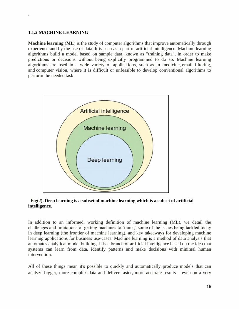
1.1.2 MACHINE LEARNING

Machine learning (ML) is the study of computer algorithms that improve automatically through

experience and by the use of data. It is seen as a part of artificial intelligence. Machine learning

algorithms build a model based on sample data, known as "training data", in order to make

predictions or decisions without being explicitly programmed to do so. Machine learning

algorithms are used in a wide variety of applications, such as in medicine, email filtering,

and computer vision, where it is difficult or unfeasible to develop conventional algorithms to

perform the needed task

Fig(2). Deep learning is a subset of machine learning which is a subset of artificial

intelligence.

In addition to an informed, working definition of machine learning (ML), we detail the

challenges and limitations of getting machines to ‘think,’ some of the issues being tackled today

in deep learning (the frontier of machine learning), and key takeaways for developing machine

learning applications for business use-cases. Machine learning is a method of data analysis that

automates analytical model building. It is a branch of artificial intelligence based on the idea that

systems can learn from data, identify patterns and make decisions with minimal human

intervention.

All of these things mean it's possible to quickly and automatically produce models that can

analyze bigger, more complex data and deliver faster, more accurate results – even on a very

`

17

large scale. And by building precise models, an organization has a better chance of identifying

profitable opportunities – or avoiding unknown risks.

Classical machine learning is often categorized by how an algorithm learns to become more

accurate in its predictions. There are four basic

approaches: supervised learning, unsupervised learning, semi-supervised learning and

reinforcement learning. The type of algorithm data scientists choose to use depends on what type

of data they want to predict.

• Supervised learning:

In this type of machine learning, data scientists supply algorithms with labeled training data

and define the variables they want the algorithm to assess for correlations. Both the input and

the output of the algorithm is specified.

Examples of Supervised Learning: Regression, Decision Tree, Random Forest, KNN,

Logistic Regression etc.

• Unsupervised learning:

This type of machine learning involves algorithms that train on unlabeled data. The algorithm

scans through data sets looking for any meaningful connection. The data that algorithms train

on as well as the predictions or recommendations they output are predetermined.

Examples of Unsupervised Learning: Apriori algorithm, K-means.

• Semi-supervised learning:

This approach to machine learning involves a mix of the two preceding types. Data scientists

may feed an algorithm mostly labeled training data, but the model is free to explore the data

on its own and develop its own understanding of the data set.

• Reinforcement learning:

Data scientists typically use reinforcement learning to teach a machine to complete a multi-

step process for which there are clearly defined rules. Data scientists program an algorithm to

`

18

complete a task and give it positive or negative cues as it works out how to complete a task.

But for the most part, the algorithm decides on its own what steps to take along the way.

Example of Reinforcement Learning: Markov Decision Process.

1.1.3 DATA PREPROCESSING

There are seven significant steps in data pre-processing in Machine Learning:

1. Acquire the dataset

To build and develop Machine Learning models, you must first acquire the relevant dataset. This

dataset will be comprised of data gathered from multiple and disparate sources which are then

combined in a proper format to form a dataset. Dataset formats differ according to use cases

2. Import all the crucial libraries

Since Python is the most extensively used and also the most preferred library by Data Scientists

around the world, we’ll show you how to import Python libraries for data preprocessing in

Machine Learning. Read more about Python libraries for Data Science here. The predefined

Python libraries can perform specific data preprocessing jobs. The three core Python libraries

used for this data preprocessing in Machine Learning are:

• NumPy

NumPy is the fundamental package for scientific calculation in Python. Hence, it is used for

inserting any type of mathematical operation in the code. Using NumPy, you can also add large

multidimensional arrays and matrices in your code.

• Pandas

Pandas is an excellent open-source Python library for data manipulation and analysis. It is

extensively used for importing and managing the datasets. It packs in high-performance, easy-to-

use data structures and data analysis tools for Python.

• Matplotlib

Matplotlib is a Python 2D plotting library that is used to plot any type of charts in Python. It can

deliver publication-quality figures in numerous hard copy formats and interactive environments

across platforms (IPython shells, Jupyter notebook, web application servers, etc.).

3. Import the dataset

In this step, you need to import the dataset/s that you have gathered for the ML project at hand.

However, before you can import the dataset/s, you must set the current directory as the working

`

19

directory. Once you’ve set the working directory containing the relevant dataset, you can import

the dataset using the “read_csv()” function of the Pandas library. This function can read a CSV

file (either locally or through a URL) and also perform various operations on it. The read_csv()

is written as:

data_set= pd.read_csv(‘Dataset.csv’)

4. Identifying and handling the missing values

In data preprocessing, it is pivotal to identify and correctly handle the missing values, failing to

do this, you might draw inaccurate and faulty conclusions and inferences from the data. Needless

to say, this will hamper your ML project.

Basically, there are two ways to handle missing data:

• Deleting a particular row – In this method, you remove a specific row that has a null value for

a feature or a particular column where more than 75% of the values are missing. However, this

method is not 100% efficient, and it is recommended that you use it only when the dataset has

adequate samples. You must ensure that after deleting the data, there remains no addition of

bias.

• Calculating the mean – This method is useful for features having numeric data like age, salary,

year, etc. Here, you can calculate the mean, median, or mode of a particular feature or column or

row that contains a missing value and replace the result for the missing value. This method can

add variance to the dataset, and any loss of data can be efficiently negated. Hence, it yields better

results compared to the first method (omission of rows/columns). Another way of approximation

is through the deviation of neighbouring values. However, this works best for linear data.

5. Encoding the categorical data

Categorical data refers to the information that has specific categories within the dataset. In the

dataset cited above, there are two categorical variables – country and purchased.

Machine Learning models are primarily based on mathematical equations. Thus, you can

intuitively understand that keeping the categorical data in the equation will cause certain issues

since you would only need numbers in the equations.

6. Splitting the dataset

Every dataset for Machine Learning model must be split into two separate sets – training set and

test set.

`

20

Training set denotes the subset of a dataset that is used for training the machine learning model.

Here, you are already aware of the output. A test set, on the other hand, is the subset of the

dataset that is used for testing the machine learning model. The ML model uses the test set to

predict outcomes.

7. Feature scaling

Feature scaling marks the end of the data preprocessing in Machine Learning. It is a method

to standardize the independent variables of a dataset within a specific range. In other words,

feature scaling limits the range of variables so that you can compare them on common grounds.

1.1.4 DATA MINING

The process of extracting information to identify patterns, trends, and useful data that would

allow the business to take the data-driven decision from huge sets of data is called Data Mining.

In other words, we can say that Data Mining is the process of investigating hidden patterns of

information to various perspectives for categorization into useful data, which is collected and

assembled in particular areas such as data warehouses, efficient analysis, data mining algorithm,

helping decision making and other data requirement to eventually cost-cutting and generating

revenue.

Data mining is the act of automatically searching for large stores of information to find trends

and patterns that go beyond simple analysis procedures. Data mining utilizes complex

mathematical algorithms for data segments and evaluates the probability of future events. Data

Mining is also called Knowledge Discovery of Data (KDD).

Data mining works in conjunction with predictive analysis, a branch of statistical science that

uses complex algorithms designed to work with a special group of problems. The predictive

analysis first identifies patterns in huge amounts of data, which data mining generalizes for

predictions and forecasts. Data mining serves a unique purpose, which is to recognize patterns in

datasets for a set of problems that belong to a specific domain.

Fig(3).Data Mining involves of Statistics, Artificial Intelligence, Machine Learning

`

21

We can also define data mining as a technique of investigation patterns of data that belong to

particular perspectives. This helps us in categorizing that data into useful information. This

useful information is then accumulated and assembled to either be stored in database servers, like

data warehouses, or used in data mining algorithms and analysis to help in decision making.

Moreover, it can be used for revenue generation and cost-cutting amongst other purposes.

Advantages of Data Mining

• The Data Mining technique enables organizations to obtain knowledge-based data.

• Data mining enables organizations to make lucrative modifications in operation and

production.

• Compared with other statistical data applications, data mining is a cost-efficient.

• Data Mining helps the decision-making process of an organization.

• It Facilitates the automated discovery of hidden patterns as well as the prediction of

trends and behaviours.

• It can be induced in the new system as well as the existing platforms.

• It is a quick process that makes it easy for new users to analyze enormous amounts of

data in a short time.

Data Mining Applications

• Data Mining in Healthcare

• Data Mining in Market Basket Analysis

• Data mining in Education

• Data Mining in Manufacturing Engineering

• Data Mining in CRM (Customer Relationship Management)

• Data Mining in Fraud detection

• Data Mining in Lie Detection

• Data Mining Financial Banking

`

22

1.1.5 PYTHON

Python is a popular object-oriented programming language having the capabilities of high-level

programming language. Its easy to learn syntax and portability capability makes it popular these

days. The following facts given us the introduction to Python

Python was developed by Guido van Rossum at Stichting Mathematisch Centrum in the

Netherlands.

It was written as the successor of programming language named ‘ABC’.

Its first version is released in 1991.

The name Python was picked by Guido van Rossum from a TV show named Monty Python’s

Flying Circus.

It is an open source programming language which means that we can freely download it and use

it to develop programs. It can be downloaded from www.python.org..

Python programming language is having the features of Java and C both. It is having the elegant

‘C’ code and on the other hand, it is having classes and objects like java for object-oriented

programming

It is an interpreted language, which means the source code of Python program would be first

converted into bytecode and then executed by Python virtual machine.

Why to learn “Python?

Python is a high-level, interpreted, interactive and object-oriented scripting language. Python is

designed to be highly readable. It uses English keywords frequently where as other languages

use punctuation, and it has fewer syntactical constructions than other language

Python is a MUST for students and working professionals to become a great Software Engineer

specially when they are working in Web Development Domain. I will list down some of the key

advantages of learning Python

Python is Interpreted − Python is processed at runtime by the interpreter. You do not need to

compile your program before executing it. This is similar to PERL and PHP

Python is Interactive − You can actually sit at a Python prompt and interact with the interpreter

directly to write your programs.

Python is Object-Oriented − Python supports Object-Oriented style or technique of

programming that encapsulates code within objects

`

23

Python is a Beginner's Language − Python is a great language for the beginner level

programmers and supports the development of a wide range of applications from simple text

processing to WWW browsers to games

Characteristics of Python

Following are important characteristics of Python Programming

• It supports functional and structured programming methods as well as OOP.

• It can be used as a scripting language or can be compiled to byte-code for building

large applications.

• It provides very high-level dynamic data types, supports dynamic type checking.

• It supports automatic garbage collection.

• It can be easily integrated with C, C++, COM, ActiveX, CORBA, and Java.

Applications of Python

As mentioned before, Python is one of the most widely used language over the web. I'm going to

list few of them here:

Easy-to-learn − Python has few keywords, simple structure, and a clearly defined syntax. This

allows the student to pick up the language quickly

Easy-to-read − Python code is more clearly defined and visible to the eyes

Easy-to-maintain - Python's source code is fairly easy-to-maintain

A broad standard library − Python's bulk of the library is very portable and cross platform

compatible on UNIX, Windows, and Macintosh

Interactive Mode − Python has support for an interactive mode which allows interactive testing

and debugging of snippets of code

Portable − Python can run on a wide variety of hardware platforms and has the same inteterface

on all platforms

`

24

GUI Programming − Python supports GUI applications that can be created and ported to many

system calls, libraries and windows systems, such as Windows MFC, Macintosh, and the X

Window system of Unix

Scalable − Python provides a better structure and support for large programs than shell scripting

NUMPY

NumPy is one of the most powerful Python libraries. It is used in the industry for array

computing. This article will outline the core features of the NumPy library. It will also provide an

overview of the common mathematical functions in an easy-to-follow manner. Numpy is gaining

popularity and is being used in a number of production systems.

PANDAS

pandas is a software library written for the Python programming language for data manipulation

and analysis. In particular, it offers data structures and operations for manipulating numerical

tables and time series. It is free software released under the three-clause BSD license. The name

is derived from the term "panel data", an econometrics term for data sets that include

observations over multiple time periods for the same individuals.

• Data Frame object for data manipulation with integrated indexing.

• Tools for reading and writing data between in-memory data structures and different file

formats.

• Data alignment and integrated handling of missing data.

• Reshaping and pivoting of data sets.

• Dataset merging and joining

.

DJANGO

Django is a high-level Python web framework that enables rapid development of secure and

maintainable websites. Built by experienced developers, Django takes care of much of the hassle

of web development, so you can focus on writing your app without needing to reinvent the

wheel.

Django helps you write software that is:

• Complete

• Versatile

• Secure

• Scalable

• Maintainable

• portable

`

25

SKLEARN

Scikit-learn is probably the most useful library for machine learning in Python. The sklearn

library contains a lot of efficient tools for machine learning and statistical modeling including

classification, regression, clustering and dimensionality reduction.

Components of scikit-learn: • Supervised learning algorithms

• Cross-validation

• Unsupervised learning algorithms

• Various toy datasets

• Feature extraction

MATPLOTLIB

Matplotlib is a plotting library for the Python programming language and its numerical

mathematics extension NumPy. Matplotlib is one of the most popular Python packages used for

data visualization. It is a cross-platform library for making 2D plots from data in arrays. It

provides an object-oriented API that helps in embedding plots in applications using Python GUI

toolkits such as PyQt, WxPythonotTkinter. It can be used in Python and IPython shells, Jupyter

notebook and web application servers also.

PICKLE

Pickle in Python is primarily used in serializing and deserializing a Python object structure. In

other words, it’s the process of converting a Python object into a byte stream to store it in a

file/database, maintain program state across sessions, or transport data over the network.

You can pickle objects with the following data types:

• Booleans

• Integers

• Floats

• Complex numbers

• (normal and Unicode) Strings

• Tuples

• Lists

• Sets

• Dictionaries that obtain picklable object

`

26

1.2 MOTIVATION OF THE WORK

In this project we tried to develop a system for personality prediction using Big five personality

traits and also to evaluate the personality type of the person. The personality of the human

plays a major role in his personal and professional life. Now a days many organizations

started short listing the candidate based upon their personality as this increases the

efficiency of work because the person is working in what he is good and at what he is

forced to do.

Personality test are used by many companies during the hiring process. They are designed

to help employees gain more insight into each candidate work style and performances. Not

only the skills but also good personality is important for the companies to hire. So that this

project will helps the people who are attending for hiring process. Persons can take the

personality test and can improve the skills required for the company.

Daily so many students are writing competitive exams that mainly focuses on personality

The main motives of that exams is to check the students personality and skills. This project

will helps to write the personality test and check the personality of the person. From the

personality classification person can view the type of personality and can improve the

personality based upon the results.

The Big five personality model is a model which gives the personality of each person.

.

`

27

1.3 PROBLEM STATEMENT

• Now a days personality assessment has become the most used test to hire many

employees

• Classifying the personality of the user based on the big five personality traits using

data mining

• We need a strong model that predicts personality of people based on their

imagination and thoughts. The goal of this project is to build a model that predicts

the personality of the people.

• The main aim of the proposed system is to predict the personality of the user by the

answers given by the user. The project is aimed to developing software which will be

helpful in identifying the personality of the person. It uses the concept of machine

learning algorithms

• After classification is done the user type personality will be displayed.

`

28

CHAPTER 2: LITERATURE SURVEY

2.1. Novel approaches to automated personality classification:

This project [4] proposes several new research directions regarding the problem of Automated

Personality Classification (APC). Firstly, we investigate possible improvements of the existing

solutions to the problem of APC, for which we use different combinations of the APC corpora,

psychological trait measurements, and learning algorithms. Afterwards, we consider extensions

of the APC problem and the related tasks, such as dynamical APC and detecting personality

inconsistency in a text. This entire research was performed in the context of social networks and

the related data mining mechanisms. Personality classification is one of the problems considered

by personality psychology, a branch of psychology. The focus of this field is the study of

personality and individual differences. According to that study, personality can be defined as a

dynamic and organized set of characteristics of a person, which have a unique influence on

cognition, motivation and behaviour of that person. In this paper the problem of automated

personality classification is considered based on information from the following content: textual

content that the person wrote and meta information about a person received on request, through

social networks or other means. There are studies that also include speech, analysis of facial

characteristics, gestures and other aspects of behaviour, but they are not the subjects of our study.

The standard approach to solving the APC problem based on the aforementioned content is

described in the following steps: A) Gathering the corpus data. B) Determination of the

personality characteristics of the participants, and C) Building the model.

2.2. Educational Game (Detecting personality of players in an educational game):

One of the goals of Educational Data Mining [1] is to develop the methods for student modelling

based on educational data, such as; chat conversation, class discussion, etc. On the other hand,

individual behaviour and personality play a major role in Intelligent Tutoring Systems (ITS) and

Educational Data Mining (EDM). Thus, to develop a user adaptable system, the student’s

behaviours that occurring during interaction has huge impact EDM and ITS. In this chapter, we

introduce a novel data mining techniques and natural language processing approaches for

automated detection student’s personality and behaviours in an educational game (Land Science)

where students act as interns in an urban planning firm and discuss in groups their ideas. In order

to apply this framework, input excerpts must be classified into one of six possible personality

classes. We applied this personality classification method using machine learning algorithms,

such as: Naive Bayes, Support Vector Machine (SVM) and Decision Tree.

There are different traditional and manual techniques for the detection of psychopathy, and these

are listed as follows: the Hare Psychopathy Checklist [22], Wmatrix linguistics analysis [9],

Welsh Anxiety Scale [1], Psychopathy Checklist-Revised (PCL-R), Wide Range Achievement

Test [11], Self-Report Psychopathy Test III (SRP-III) [10], Wonderlic Personnel Test, Levenson

Self-Report Psychopathy Scale (LSRP) [26], and Dictionary of Affect in Language (DAL) [9].

However, online users of social network websites express themselves using texts, images, public

`

29

profiles, and status updates [14]. The social media-based textual content can also be investigated

to detect and authenticate the personality traits of an individual, specifically a psychopath's

behaviour.

Some studies applied supervised machine learning approaches for the classification of

psychopathy. For example, Keshtkar et al. [14] exploited different machine learning algorithms,

namely, (i) SVM, (ii) NB, and (iii) DT, where the main emphasis of the proposed system was to

automatically identify the personality traits of students in an educational game. The experimental

results showed that the n-gram gave the best performance compared with the other feature sets.

2.3. A System for Personality and Happiness Detection:

This[3] work proposes a platform for estimating personality and happiness. Starting from

Eysenck's theory about human's personality, authors seek to provide a platform for collecting

text messages from social media (WhatsApp), and classifying them into different personality

categories. Although there is not a clear link between personality features and happiness, some

correlations between them could be found in the future. In this work, we describe the platform

developed, and as a proof of concept, we have used different sources of messages to see if

common machine learning algorithms can be used for classifying different personality features

and happiness. Researchers have tried to obtain information about the personality of human

beings through direct means such as the EPQ-R questionnaire, but they have also used indirect

methods. Because personality is considered to be stable over time and throughout different

situations, specialized psychologists are able to infer the personality profile of a subject by

observing the subject’s behaviour. One of the sources of knowledge about the behaviour of

individuals is written text According to research in this field, it is reasonable to expect that

different individuals will have different ways of expressing themselves through the written word,

and these differences will correspond to their individual

2.4. Using Twitter Content to Predict Psychopathy:

An ever-growing number of users share their thoughts and experiences using the Twitter micro

logging service. Although sometimes dismissed as containing too little content to convey

significant information, these messages can be combined to build a larger picture of the user

posting them. One particularly notable personality trait which can be discovered this way is

psychopathy: the tendency for disregarding others and the rule of society. In this paper, we

explore techniques to apply data mining towards the goal of identifying those who score in the

top 1.4% of a well known psychopathy metric using information available from their Twitter

accounts. We apply a newly proposed form of ensemble learning, Select RUSBoost (which adds

feature selection to our earlier imbalance aware ensemble in order to resolve high

dimensionality), employ four classification learners, and use four feature selection techniques.

The results show that when using the optimal choices of techniques, we are able to achieve an

AUC value of 0.736. Furthermore, these results were only achieved when using the Select

RUSBoost technique, demonstrating the importance of feature selection, data sampling, and

ensemble learning. Overall, we show[2] that data mining can be a valuable tool for law

enforcement and others interested in identifying abnormal psychiatric states from Twitter data.

`

30

R. Wald et. al.[3] have used social media like twitter contents to identify human psychology.

They said Twitter, a micro blogging site, is used by a number of users to share their experiences

and thoughts about their day-to-day life. Although researchers have often discarded the method

of predicting personality by analyzing the tweets because they are of the view that it contains

very little content to predict significant information, but these tweets can be combined to make a

larger picture of the user who is posting them. Select RUSBoost, a new form of ensemble

learning has been used to predict psychopathy using Twitter, which uses four classification

learners and four feature selection techniques.

2.5 An Examination of Online learning effectiveness using data mining

Nurbiha A Shukora [4] have given the concept of Online learning which became highly popular

because of technological advancement that made it possible to have discussions even from a

distance. Most studies have reported that have been conducted report how effective online

learning has helped students to improve their learning power while assessing the learning process

simultaneously . This kind of discussion can be possible only by applying data mining technique

where we can access the different experiences of students which they filed online on basis of

their log files . However , it is said that students should put more hard work to become an

excellent online learner .

`

31

CHAPTER 3: PROPOSED METHODOLOGY

3.1 INTRODUCTION

To overcome the problems of the existing system an Automated personality classification

system is proposed which uses some data mining techniques and machine learning algorithms

are used to classify the personalities of different users.

And by using different algorithms like Big Five Personality Model, Logistic regression, Decision

Tree and Support Vector Machine. By identifying the past data and their patterns it is easy to

identify the personality by applying new techniques, so it overcomes the existing system. In this

proposed system, the graph will give percentages of this Automated Personality System. Here it

gives probabilistic values from 0 to 1. An Automated Personality Classification System is

designed in which every applicant/user is given a separate username and password if registered

or else user has to get registered before taking the survey. Each applicant logins the survey /test

using his /her username and password and takes the survey. It consists of 50 questions of each

trait and aptitude test of 10 questions, and the user can take the survey so that it determines the

Big five personality traits. After taking the survey user can see the result of his/her personality.

Thus we can see the graph after getting result and then it give suggestions to those whose

personality matches i.e., , like friend suggestion .

By this, it is useful for many sectors like interview, recruitment process, government sectors,

psychometric tests, and once a user results are suitable then can get into any organization which

is based on personality type jobs.

In this system we are finding the personality of the each user and the average of each big five

personality trait average out of 10 and finally getting the personality type of the user.

Based up on the answers given by the user in personality test the type of the personality is

predicted.

By that personality type predicted user can easily apply for the job and can know the personality

predicted. In the same way students can also know their personality and can participate in the

competitive exams.

`

32

3.2 SYSTEM ARCHITECTURE

Fig(4). The Architecture gives us an idea on how the system works.

The system architecture gives an overview of the working of the system. The working of the

system starts with the collection of data from the data base and here we divide the data into

training data and testing data, selecting the attributes. And then pre-processing the required data

is done so that the it removes duplicate data and the error data. Firstly user have to login and then

write the personality test there are 50 questions each trait consists of 10 questions, user have to

answer those 50 questions, based up on the answers the algorithms are applied and the model is

trained using the training data .Here we are big five personality traits and then classify the

personality type. Accuracy is measured by testing the system using testing data. So, after that

Personality is predicted.

`

33

CHAPTER 4: EXPERIMENTAL ANALYSIS AND RESULTS

4.1 MODULE DIVISION

Module Division is the process of dividing collection of source files required in the project

into discrete units of functionality. Each module can be independently built, tested and

debugged. Below are the modules which are divided in our project.

1.Data collection

2.Attribute selection

3.Pre-processing of data

4.Prediction of personality

4.1.1 Data Collection

First step for prediction system is data collection and deciding about the training and testing

dataset. In this project we have imported dataset from Kaggle website which includes 70% of

training dataset and 30% of testing dataset. Data collection is defined as the procedure of

collecting, measuring and analyzing accurate insights for research using standard validated

techniques. A researcher can evaluate their hypothesis on the basis of collected data. In most

cases, data collection is the primary and most important step for research, irrespective of the field

of research. The approach of data collection is different for different fields of study, depending

on the required information.

TRAINING DATASET:

In a dataset, a training set is implemented to build up a model, while a test (or validation) set is to

validate the model built. Here, you have the complete training dataset. You can extract features

and train to fit a model and so on.

TESTING DATASET:

Here, once the model is obtained, you can predict using the model obtained on the training set.

Some data may be used in a confirmatory way, typically to verify that a given set of input to a

given function produces some expected result. Other data may be used in order to challenge the

ability of the program to respond to unusual, extreme, exceptional, or unexpected input.

`

34

4.1.2 Attribute Selection

Attribute of dataset are property of dataset which are used for system and for personality many

attributes are like heart gender of the person, age of the person ,Big five traits like Openness,

Neuroticism, Extraversion, Agreeableness, Consciousness( value 1 -10). The importance of

feature selection can best be recognized when you are dealing with a dataset that contains a vast

number of features. This type of dataset is often referred to as a high dimensional dataset. Now,

with this high dimensionality, comes a lot of problems such as - this high dimensionality will

significantly increase the training time of your machine learning model, it can make your model

very complicated which in turn may lead to Overfitting.

4.1.3 Pre-Processing of Data

Pre-processing needed for achieving best result from the machine learning algorithms. In this, we

gathered dataset and it was pre-processed before it is sent to training stage. Sampling is a very

common method for selecting a subset of the dataset that we are analysing. In most cases,

working with the complete dataset can turn out to be too expensive considering the memory.

Using a sampling algorithm can help us reduce the size of the dataset to a point where we can use

a better, but more expensive, machine learning algorithm. When we talk about data, we usually

think of some large datasets with huge number of rows and columns. While that is a likely

scenario, it is not always the case — data could be in so many different forms: Structured Tables,

Images, Audio files, Videos etc. Machines don’t understand free text, image or video data as it is,

they understand 1s and 0s. So we pre-process the data.

4.1.4 Prediction of Personality Classification

In this, system we used machine learning algorithms is performed and whichever algorithm is

used which it gives best accuracy for personality prediction. By applying all this modules finally

the personality is predicted and the final result is personality of the user.by using the training and

testing dataset the personality of the user is classified.

`

35

4.2 ALGORITHM

4.2.1 LOGISTIC REGRESSION

Logistic regression is a supervised learning classification algorithm used to predict the

probability of a target variable. The nature of target or dependent variable is dichotomous,

which means there would be only two possible classes.

o Logistic regression is one of the most popular Machine Learning algorithms, which

comes under the Supervised Learning technique. It is used for predicting the categorical

dependent variable using a given set of independent variables.

o Logistic regression predicts the output of a categorical dependent variable. Therefore the

outcome must be a categorical or discrete value. It can be either Yes or No, 0 or 1, true or

False, etc. but instead of giving the exact value as 0 and 1, it gives the probabilistic values

which lie between 0 and 1.

o Logistic Regression is much similar to the Linear Regression except that how they are

used. Linear Regression is used for solving Regression problems, whereas Logistic

regression is used for solving the classification problems.

o In Logistic regression, instead of fitting a regression line, we fit an "S" shaped logistic

function, which predicts two maximum values (0 or 1).

o The curve from the logistic function indicates the likelihood of something such as

whether the cells are cancerous or not, a mouse is obese or not based on its weight, etc.

o Logistic Regression is a significant machine learning algorithm because it has the ability

to provide probabilities and classify new data using continuous and discrete datasets.

o Logistic Regression can be used to classify the observations using different types of data

and can easily determine the most effective variables used for the classification. The

below image is showing the logistic function:

Fig(5). Logistic Regression Curve

`

36

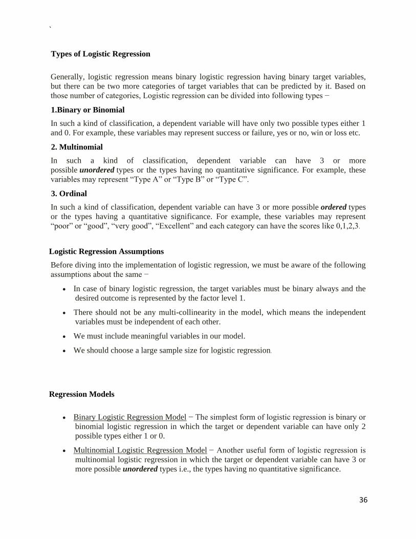
Types of Logistic Regression

Generally, logistic regression means binary logistic regression having binary target variables,

but there can be two more categories of target variables that can be predicted by it. Based on

those number of categories, Logistic regression can be divided into following types −

1.Binary or Binomial

In such a kind of classification, a dependent variable will have only two possible types either 1

and 0. For example, these variables may represent success or failure, yes or no, win or loss etc.

2. Multinomial

In such a kind of classification, dependent variable can have 3 or more

possible unordered types or the types having no quantitative significance. For example, these

variables may represent “Type A” or “Type B” or “Type C”.

3. Ordinal

In such a kind of classification, dependent variable can have 3 or more possible ordered types

or the types having a quantitative significance. For example, these variables may represent

“poor” or “good”, “very good”, “Excellent” and each category can have the scores like 0,1,2,3.

Logistic Regression Assumptions

Before diving into the implementation of logistic regression, we must be aware of the following

assumptions about the same −

• In case of binary logistic regression, the target variables must be binary always and the

desired outcome is represented by the factor level 1.

• There should not be any multi-collinearity in the model, which means the independent

variables must be independent of each other.

• We must include meaningful variables in our model.

• We should choose a large sample size for logistic regression.

Regression Models

• Binary Logistic Regression Model − The simplest form of logistic regression is binary or

binomial logistic regression in which the target or dependent variable can have only 2

possible types either 1 or 0.

• Multinomial Logistic Regression Model − Another useful form of logistic regression is

multinomial logistic regression in which the target or dependent variable can have 3 or

more possible unordered types i.e., the types having no quantitative significance.

`

37

Logistic Regression Predicts Probabilities (Technical Interlude)

Logistic regression models the probability of the default class (e.g. the first class). For example,

if we are modeling people’s sex as male or female from their height, then the first class could be

male and the logistic regression model could be written as the probability of male given a

person’s height, or more formally:

P(sex=male|height)

Written another way, we are modeling the probability that an input (X) belongs to the default

class (Y=1), we can write this formally as:

P(X) = P(Y=1|X)

We’re predicting probabilities. I thought logistic regression was a classification algorithm.

Note that the probability prediction must be transformed into a binary values (0 or 1) in order to

actually make a probability prediction. More on this later when we talk about making prediction.

Logistic regression is a linear method, but the predictions are transformed using the logistic

function. continuing on from above, the model can be stated as:

p(X) = e^(b0 + b1*X) / (1 + e^(b0 + b1*X))

I don’t want to dive into the math too much, but we can turn around the above equation as

follows (remember we can remove the e from one side by adding a natural logarithm (ln) to the

other):

ln(p(X) / 1 – p(X)) = b0 + b1 * X

This is useful because we can see that the calculation of the output on the right is linear again

(just like linear regression), and the input on the left is a log of the probability of the default

class.

This ratio on the left is called the odds of the default class (it’s historical that we use odds, for

example, odds are used in horse racing rather than probabilities). Odds are calculated as a ratio of

the probability of the event divided by the probability of not the event, e.g. 0.8/(1-0.8) which has

the odds of 4. So we could instead write:

`

38

ln(odds) = b0 + b1 * X

Because the odds are log transformed, we call this left hand side the log-odds or the probit. It is

possible to use other types of functions for the transform (which is out of scope_, but as such it is

common to refer to the transform that relates the linear regression equation to the probabilities as

the link function, e.g. the probit link function.

We can move the exponent back to the right and write it as:

odds = e^(b0 + b1 * X)

All of this helps us understand that indeed the model is still a linear combination of the inputs,

but that this linear combination relates to the log-odds of the default class.

4.2.2. DECISION TREE

Decision Trees are a type of Supervised Machine Learning (that is you explain what the input is

and what the corresponding output is in the training data) where the data is continuously split

according to a certain parameter. The tree can be explained by two entities, namely decision

nodes and leaves. The leaves are the decisions or the final outcomes. And the decision nodes are

where the data is split. which are outcomes like either ‘fit’, or ‘unfit’. In this case this was a

binary classification problem (a yes no type problem). There are two main types of Decision

Trees:

1.Classification trees (Yes/No types)

What we’ve seen above is an example of classification tree, where the outcome was a variable

like ‘fit’ or ‘unfit’. Here the decision variable is Categorical.

2.Regression trees (Continuous data types)

Here the decision or the outcome variable is Continuous, e.g. a number like

123. Working Now that we know what a Decision Tree is, we’ll see how it works internally.

There are many algorithms out there which construct Decision Trees, but one of the best is called

as ID3 Algorithm. ID3 Stands for Iterative Dichotomiser 3. Before discussing the ID3

algorithm, we’ll go through few definitions. Entropy Entropy, also called as Shannon Entropy is

denoted by H(S) for a finite set S, is the measure of the amount of uncertainty or randomness in

data.

.

`

39

We’ll build a decision tree to do that using ID3 algorithm.

ID3 Algorithm will perform following tasks recursively

1. Create root node for the tree

2. If all examples are positive, return leaf node ‘positive’

3. Else if all examples are negative, return leaf node ‘negative’

4. Calculate the entropy of current state H(S)

5. For each attribute, calculate the entropy with respect to the attribute ‘x’ denoted by

H(S, x)

6. Select the attribute which has maximum value of IG(S, x)

7. Remove the attribute that offers highest IG from the set of attributes

8. Repeat until we run out of all attributes, or the decision tree has all leaf nodes.

Fig(6).Explains the general structure of a decision tree:

Decision Tree Terminologies

1.Root Node:

Root node is from where the decision tree starts. It represents the entire dataset, which further

gets divided into two or more homogeneous sets.

2.Leaf Node:

Leaf nodes are the final output node, and the tree cannot be segregated further after getting a leaf

node.

`

40

3.Splitting:

Splitting is the process of dividing the decision node/root node into sub-nodes according to the

given conditions.

4.Branch/Sub Tree:

A tree formed by splitting the tree.

5.Pruning:

Pruning is the process of removing the unwanted branches from the tree.

6.Parent/Child node:

The root node of the tree is called the parent node, and other nodes are called the child nodes.

How does the Decision Tree algorithm Work?

In a decision tree, for predicting the class of the given dataset, the algorithm starts from the root

node of the tree. This algorithm compares the values of root attribute with the record (real

dataset) attribute and, based on the comparison, follows the branch and jumps to the next node.

For the next node, the algorithm again compares the attribute value with the other sub-nodes and

move further. It continues the process until it reaches the leaf node of the tree. The complete

process can be better understood using the below algorithm:

Step-1: Begin the tree with the root node, says S, which contains the complete dataset.

Step-2: Find the best attribute in the dataset using Attribute Selection Measure (ASM).

Step-3: Divide the S into subsets that contains possible values for the best attributes.

Step-4: Generate the decision tree node, which contains the best attribute.

Step-5: Recursively make new decision trees using the subsets of the dataset created in

step -3. Continue this process until a stage is reached where you cannot further classify the

nodes and called the final node as a leaf node.

`

41

4.2.3. SUPPORT VECTOR MACHINE

Support Vector Machine or SVM is one of the most popular Supervised Learning algorithms,

which is used for Classification as well as Regression problems. However, primarily, it is used

for Classification problems in Machine Learning.

The goal of the SVM algorithm is to create the best line or decision boundary that can segregate

n-dimensional space into classes so that we can easily put the new data point in the correct

category in the future. This best decision boundary is called a hyperplane.

SVM chooses the extreme points/vectors that help in creating the hyperplane. These extreme

cases are called as support vectors, and hence algorithm is termed as Support Vector Machine.

Consider the below diagram in which there are two different categories that are classified using a

decision boundary or hyperplane:

fig(7).SVM graph

Types of SVM

SVM can be of two types:

o Linear SVM:

Linear SVM is used for linearly separable data, which means if a dataset can be

classified into two classes by using a single straight line, then such data is termed as

linearly separable data, and classifier is used called as Linear SVM classifier.

`

42

o Non-linear SVM:

Non-Linear SVM is used for non-linearly separated data, which means if a dataset

cannot be classified by using a straight line, then such data is termed as non-linear data

and classifier used is called as Non-linear SVM classifier.

Hyperplane and Support Vectors in the SVM algorithm:

Hyperplane:

There can be multiple lines/decision boundaries to segregate the classes in n-dimensional space,

but we need to find out the best decision boundary that helps to classify the data points. This best

boundary is known as the hyperplane of SVM.

The dimensions of the hyperplane depend on the features present in the dataset, which means if

there are 2 features (as shown in image), then hyperplane will be a straight line. And if there are

3 features, then hyperplane will be a 2-dimension plane.

We always create a hyperplane that has a maximum margin, which means the maximum distance

between the data points.

Support Vectors:

The data points or vectors that are the closest to the hyperplane and which affect the position of

the hyperplane are termed as Support Vector. Since these vectors support the hyperplane, hence

called a Support vector.

This is a type of machine which is basically used for analysis the data which receive from

supervised learning and identify the patterns for classification [8]. Training data set is taken and

checked that whether the test data belongs to existing class or not for personality classification

and classification.

Data is represented by Support Vector Machine model in the form of a point commonly in space

which further classified in a line or in a hyper plane. The main idea behind the support vector

machine algorithm is that if a classifier performs well at the most challenging comparisons, then

it will definitely perform even better at the most easy comparisons. Support Vector Machine

which is a nonlinear classifier often produces superior classification results than other classifier

methods. Support Vector Machine is based on non-linearly mapping the input data to some high

dimensional space where the data is separated linearly, thus giving accurate classification results.

`

43

The steps involved in Support Vector Machine are:

1. Create vectors for given question answers.

2. Then calculate the weights of the vectors.

3. Get the vectors with highest value and find value of personality

4. Finally predict personality type

PERFORMANCE METRICS

Evaluating machine learning algorithm is an essential part of a project. In this , We have used

machine learning algorithms like Logistic Regression , Support Vector Machine , Decision Tree

are used to predict the personality system. In this, we have 7 attributes and one attribute label as

personality for predicting the behaviour from the test data. Various attributes like Gender, Age,

Openness, Agreeableness, Extra version, Neuroticism or Emotional Stability, Conscientiousness

are used in this system. We have used Five Personality Traits in our system and calculated

performance metrics per each trait. We have Calculated precision, recall, f1- score, accuracy per

each trait. For each classification algorithm we will be getting the performance metrics.

Confusion Matrix

It is the easiest way to measure the performance of a classification problem where the output

can be of two or more type of classes. A confusion matrix is nothing but a table with two

dimensions viz. “Actual” and “Predicted” and furthermore, both the dimensions have “True

Positives (TP)”, “True Negatives (TN)”, “False Positives (FP)”, “False Negatives (FN)” as

shown below –

`

44

Explanation of the terms associated with confusion matrix are as follows −

True Positive: It is defined as model predicted as positive class and it is True. It is denoted by

TP.

False Positive: It is defined as model predicted as positive class and it is false. It is denoted by

FP.

False Negative: It is defined as model predicted as negative class and it is False. It is denoted by

FN.

True Negative: It is defined as model predicted as negative class and it is True. It is denoted by

TN.

Precision

It is the fraction of correctly classified instances to the total number of instances Precision, used

in document retrievals, may be defined as the number of correct documents returned by our ML

model. We can easily calculate it by confusion matrix with the help of following formula −

Precision=TP/(TP+FP)

Recall or Sensitivity

It is the fraction of correctly classified instances to the total number of instances Recall may be

defined as the number of positives returned by our ML model. We can easily calculate it by

confusion matrix with the help of following formula −

Recall=TP/(TP+FN)

Support

Support may be defined as the number of samples of the true response that lies in each class of

target values.

F1 Score

This score will give us the harmonic mean of precision and recall. Mathematically, F1 score is

the weighted average of the precision and recall. The best value of F1 would be 1 and worst

would be 0. We can calculate F1 score with the help of following formula –

F1 Score = (2* Precision*Recall)/(Precision+Recall)

F1 score is having equal relative contribution of precision and recall.

Accuracy

Accuracy is the simple ratio between number of correctly classified points to the total number of

points. It is most common performance metric for classification algorithms. It may be defined as

the number of correct predictions made as a ratio of all predictions made. We can easily

calculate it by confusion matrix with the help of following formula –

`

45

Accuracy=TP+TN/(TP+FP+FN+TN)

After performing the classification algorithms like Support Vector Machine, Decision Tree and

Logistic Regression algorithms for training and testing data we find that Decision Tree is the

Best algorithms with highest accuracy compared to both Support Vector Machine and Logistic

Regression. We found the accuracy by calculating TP, FP, FN, TN is given and using the

equation we got the accuracy. Among all the above three algorithms used, Accuracy

comparsions are :

Support vector machine : 91%

Decision Tree : 96.%

Logistic Regression : 78.%

4.3 SAMPLE CODE

import pandas as pd

from numpy import *

import numpy as np

import warnings

warnings.filterwarnings("ignore")

from sklearn import preprocessing

from sklearn import datasets, linear_model

from sklearn.metrics import mean_squared_error, r2_score

from sklearn import metrics

from sklearn.model_selection import train_test_split

from sklearn import neighbors

from sklearn import svm

from sklearn.pipeline import Pipeline

import pickle

`

46

from sklearn import tree

data = pd.read_csv('train.csv')

array = data.values

# print(array)

# processing data

for i in range(len(array)):

if array[i][0] == "Male":

array[i][0] = 1

else:

array[i][0] = 0

# print(array)

df = pd.DataFrame(array)

# print(df.head())

maindf = df[[0, 1, 2, 3, 4, 5, 6]]

mainarray = maindf.values

# print(mainarray)

temp = df[7]

# print(temp)

train_y = temp.values

# print(train_y)

# print(mainarray)

train_y = temp.values

for i in range(len(train_y)):

train_y[i] = str(train_y[i])

lables = [

`

47

"Logistic Regression",

"SVM",

"Decision Tree"

]

models = [

linear_model.LogisticRegression(multi_class='multinomial', solver='newton-cg',

max_iter=1000),

svm.SVC(kernel="poly"),

tree.DecisionTreeClassifier()

]

# mul_lr = svm.SVC(kernel="poly")

# mul_lr = Pipeline([

# ("LR", linear_model.LogisticRegression(multi_class='multinomial', solver='newton-cg',

max_iter=1000)),

# ("SVM", svm.SVC(kernel="linear"))

# ])

print("Accuracy:")

for mno in range(len(models)):

mul_lr = models[mno]

mul_lr.fit(mainarray, train_y)

# save the model to disk

pickle.dump(mul_lr, open("./model.pkl", 'wb'))

testdata = pd.read_csv('text.csv')

test = testdata.values

for i in range(len(test)):

if test[i][0] == "Male":

`

48

test[i][0] = 1

else:

test[i][0] = 0

df1=pd.DataFrame(test)

testdf =df1[[0,1,2,3,4,5,6]]

maintestarray=testdf.values

# print(maintestarray)

y_pred = mul_lr.predict(maintestarray)

# print(maintestarray[0])

# print(list(y_pred), df1[[7]].values)

real = df1[[7]].values

predicted = list(y_pred)

error = 0

for i in range(len(predicted)):

if (real[i][0] != predicted[i]): error += 1

print(lables[mno]+":", ((len(predicted) - error)/len(predicted))*100)

for i in range(len(y_pred)) :

y_pred[i]=str((y_pred[i]))

DF = pd.DataFrame(y_pred,columns=['Predicted Personality.'])

DF.index=DF.index+1

DF.index.names = ['Person No']

DF.to_csv("output.csv")

`

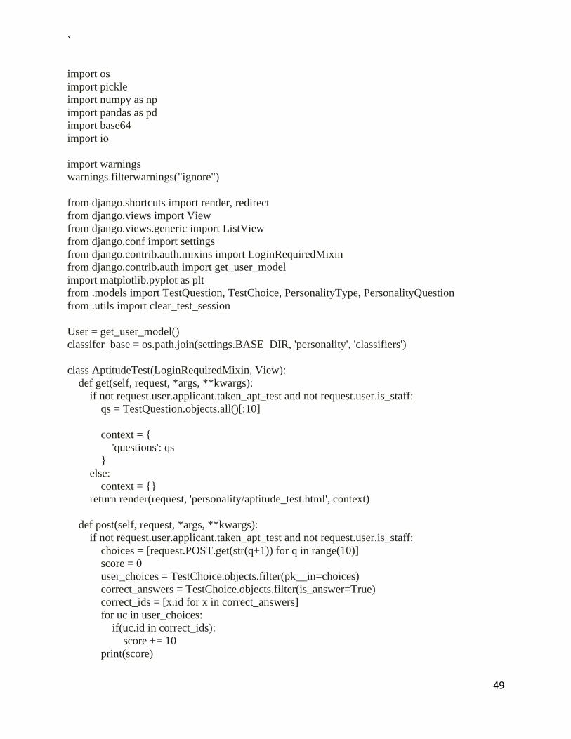
49

import os

import pickle

import numpy as np

import pandas as pd

import base64

import io

import warnings

warnings.filterwarnings("ignore")

from django.shortcuts import render, redirect

from django.views import View

from django.views.generic import ListView

from django.conf import settings

from django.contrib.auth.mixins import LoginRequiredMixin

from django.contrib.auth import get_user_model

import matplotlib.pyplot as plt

from .models import TestQuestion, TestChoice, PersonalityType, PersonalityQuestion

from .utils import clear_test_session

User = get_user_model()

classifer_base = os.path.join(settings.BASE_DIR, 'personality', 'classifiers')

class AptitudeTest(LoginRequiredMixin, View):

def get(self, request, *args, **kwargs):

if not request.user.applicant.taken_apt_test and not request.user.is_staff:

qs = TestQuestion.objects.all()[:10]

context = {

'questions': qs

}

else:

context = {}

return render(request, 'personality/aptitude_test.html', context)

def post(self, request, *args, **kwargs):

if not request.user.applicant.taken_apt_test and not request.user.is_staff:

choices = [request.POST.get(str(q+1)) for q in range(10)]

score = 0

user_choices = TestChoice.objects.filter(pk__in=choices)

correct_answers = TestChoice.objects.filter(is_answer=True)

correct_ids = [x.id for x in correct_answers]

for uc in user_choices:

if(uc.id in correct_ids):

score += 10

print(score)

`

50

user = User.objects.get(username=request.user.username)

user.applicant.test_score = score

user.applicant.taken_apt_test = True

user.applicant.save()

return redirect('aptitude_finished')

else:

return render(request, 'personality/aptitude_test.html', {})

class PersonalityTest(LoginRequiredMixin, View):

def get(self, request, *args, **kwargs):

if not request.user.applicant.taken_personality_test and not request.user.is_staff:

qs = PersonalityType.objects.all()

type_o = PersonalityType.objects.get(id=1)

type_c = PersonalityType.objects.get(id=2)

type_e = PersonalityType.objects.get(id=3)

type_a = PersonalityType.objects.get(id=4)

type_n = PersonalityType.objects.get(id=5)

context = {

'type_o': type_o,

'type_c': type_c,

'type_e': type_e,

'type_a': type_a,

'type_n': type_n,

}

else:

context = {}

return render(request, 'personality/personality_test.html', context)

def post(self, request, *args, **kwargs):

if not request.user.applicant.taken_personality_test and not request.user.is_staff:

request_count = len(request.POST)-2

# print(request.POST, request_count)

choices = [int(request.POST.get('choice'+str(q+1))) for q in range(request_count)]

print(choices)

average = int(sum(choices)/2.5) if len(choices) > 0 else 0

print(average)

type_o = PersonalityType.objects.get(id=1)

type_c = PersonalityType.objects.get(id=2)

type_e = PersonalityType.objects.get(id=3)

type_a = PersonalityType.objects.get(id=4)

type_n = PersonalityType.objects.get(id=5)

user = User.objects.get(username=request.user.username)

`

51

test_type = request.POST.get('test_type')

if test_type == '1':

print('Openness Test')

request.session['avg_o'] = sum(choices)/len(choices)

pickle_in = open(os.path.join(classifer_base, 'openness.pkl'), 'rb')

clf_opn = pickle.load(pickle_in)

answers = pd.DataFrame([choices])

result = clf_opn.predict(answers)

user.applicant.personality.add(type_o) if result == ['YES'] else None

print('Openness', result)

request.session['done_o'] = True

elif test_type == '2':

print('Consientious Test')

request.session['avg_c'] = sum(choices)/len(choices)

pickle_in = open(os.path.join(classifer_base, 'conscientious.pkl'), 'rb')

clf_con = pickle.load(pickle_in)

answers = pd.DataFrame([choices])

result = clf_con.predict(answers)

user.applicant.personality.add(type_c) if result == ['YES'] else None

print('Conscientious', result)

request.session['done_c'] = True

elif test_type == '3':

print('Extroversion Test')

request.session['avg_e'] = sum(choices)/len(choices)

pickle_in = open(os.path.join(classifer_base, 'extroversion.pkl'), 'rb')

clf_ext = pickle.load(pickle_in)

answers = pd.DataFrame([choices])

result = clf_ext.predict(answers)

user.applicant.personality.add(type_e) if result == ['YES'] else None

print('Extroversion', result)

request.session['done_e'] = True

elif test_type == '4':

print('Agreeable Test')

request.session['avg_a'] = sum(choices)/len(choices)

pickle_in = open(os.path.join(classifer_base, 'agreeable.pkl'), 'rb')

clf_agb = pickle.load(pickle_in)

answers = pd.DataFrame([choices])

result = clf_agb.predict(answers)

user.applicant.personality.add(type_a) if result == ['YES'] else None

print('Agreeable', result)

request.session['done_a'] = True

elif test_type == '5':

print('Neurotism Test')

request.session['avg_n'] = sum(choices)/len(choices)

pickle_in = open(os.path.join(classifer_base, 'neurotism.pkl'), 'rb')

`

52

clf_neu = pickle.load(pickle_in)

answers = pd.DataFrame([choices])

result = clf_neu.predict(answers)

user.applicant.personality.add(type_n) if result == ['YES'] else None

print('Neurotism', result)

request.session['done_n'] = True

user.applicant.taken_personality_test = True

user.applicant.save()

return redirect('personality_completed')

return redirect('personality_test')

class PersonalityCompleted(LoginRequiredMixin, View):

def get(self, request, *args, **kwargs):

blob = None

personality = None

completed = True

if request.user.applicant.taken_personality_test and not request.user.is_staff:

pickle_in = open(os.path.join(classifer_base, 'employability.pkl'), 'rb')

clf_emp = pickle.load(pickle_in)

if (request.session.get('avg_o', None) == None):

completed = False

if (completed):

avg_o = request.session.get('avg_o', None)*2

avg_c = request.session.get('avg_c', None)*2

avg_e = request.session.get('avg_e', None)*2

avg_a = request.session.get('avg_a', None)*2

avg_n = request.session.get('avg_n', None)*2

averages = [avg_o, avg_c, avg_e, avg_a, avg_n]

# averages = [avg_o*2, avg_c*2, avg_e*2, avg_a*2, avg_n*2]

# averages = [3.1, 3.1, 3.2, 3.2, 1.9]

print(averages)

if len(averages) != 5 or None in averages:

completed = False

else:

personality_avgs = pd.DataFrame([averages])

result = clf_emp.predict(personality_avgs)

print('Employable', result)

possible_results = [1,0]

if result in possible_results:

completed = True

print('openness',avg_o)

`

53

print('consciencitousness', avg_c)

print('extraversion',avg_e)

print('agreebleness',avg_a)

print('neutroticism', avg_n)

print("Averages", averages)

model = open(os.path.join(classifer_base, 'model.pkl'), 'rb')

model = pickle.load(model)

# yy=[int(avg_o*1.8), int(avg_c*1.8), int(avg_e*1.8), int(avg_a*1.8),

int(avg_n*1.8)]

# avg_tmp = []

# for Current_avg in averages:

# avg_tmp.append(int(Current_avg))

# avg2 = [avg_o*2, avg_c*2, avg_e*2, avg_a*2, avg_n*2]

personality = model.predict([averages])[0]

# print("Avg...", avg_tmp)

# print("Personality:", personality[0])

# blob = base64.b64encode(open('../output.jpg', 'rb').read())

# blob = 'data:image/jpeg;base64,' + str(blob)[2:-1]

nn=[' Openness ',' Conscientiousness ',' Extraversion ',' Agreeableness ','

Neuroticism ']

yy=[avg_o, avg_c, avg_e, avg_a, avg_n]

plt.bar(nn,yy)

plt.xticks(rotation=15)

# plt.savefig("output.jpg")

iobytes = io.BytesIO()

plt.savefig(iobytes, format='jpg')

iobytes.seek(0)

blob = base64.b64encode(iobytes.read())

blob = 'data:image/jpeg;base64,' + str(blob)[2:-1]

plt.close()

clear_test_session(request)

user = User.objects.get(username=request.user.username)

user.applicant.is_employable = True if result == [1] else False

user.applicant.save()

else:

completed = False

else:

completed = False

context = {

`

54

'completed': completed,

'image': blob,

'personality': personality

}

return render(request, 'personality/personality_completed.html', context)

from django.contrib import admin

from django.contrib.auth.admin import UserAdmin

from django.contrib.auth import get_user_model

from django.contrib.auth.models import Group

from django.conf import settings

from .models import Applicant

User = get_user_model()

class ApplicantInline(admin.StackedInline):

model = Applicant

can_delete = False

verbose_name_plural = 'Applicant'

fk_name = 'user'

class CustomUserAdmin(UserAdmin):

inlines = (ApplicantInline, )

list_display = ('username', 'email', 'is_staff', 'get_employable')

list_select_related = ('applicant', )

fieldsets = (

(None, {'fields': ('email', 'password')}),

('Personal info', {'fields': ('username', 'first_name', 'last_name',)}),

('Permissions', {'fields': ('is_active', 'is_staff', 'is_superuser',)}),

)

def get_employable(self, instance):

return instance.applicant.is_employable

get_employable.short_description = 'Is Employable'

admin.site.unregister(User)

admin.site.register(User, CustomUserAdmin)

admin.site.unregister(Group)

`

55

from django.shortcuts import render

from django.contrib.auth.forms import UserCreationForm

from django.views.generic import CreateView

from django.conf import settings

from .forms import ApplicantRegisterForm

User = settings.AUTH_USER_MODEL

class RegisterView(CreateView):

# model = User

form_class = ApplicantRegisterForm

template_name = 'accounts/register.html'

success_url = '/login'

"""django_project URL Configuration

The `urlpatterns` list routes URLs to views. For more information please see:

https://docs.djangoproject.com/en/2.0/topics/http/urls/

Examples:

Function views

1. Add an import: from my_app import views

2. Add a URL to urlpatterns: path('', views.home, name='home')

Class-based views

1. Add an import: from other_app.views import Home

2. Add a URL to urlpatterns: path('', Home.as_view(), name='home')

Including another URLconf

1. Import the include() function: from django.urls import include, path

2. Add a URL to urlpatterns: path('blog/', include('blog.urls'))

"""

from django.contrib import admin

from django.urls import path, include

from django.views.generic import TemplateView

from .views import Home

urlpatterns = [

path('admin/', admin.site.urls),

path('', Home.as_view(), name='home'),

path('about/', TemplateView.as_view(

template_name='about_us.html'

), name='about_us'),

path('personality/', include('personality.urls')),

path('', include('accounts.urls')),

import base64

`

56

import matplotlib.pyplot as plt

import io

nn=[' openness ',' consciencitousness ',' extraversion ',' agreebleness ',' neutroticism ']

yy=[4, 6, 3, 2, 5]

plt.bar(nn,yy)

iobytes = io.BytesIO()

plt.savefig(iobytes, format='jpg')

iobytes.seek(0)

blob = base64.b64encode(iobytes.read())

blob = 'data:image/jpeg;base64,' + str(blob)[2:-1]

print(blob)

# print(my_base64_jpgData)

# plt.show()

# blob = base64.b64encode(open('./output.jpg', 'rb').read())

# blob = 'data:image/jpeg;base64,' + str(blob)[2:-1]

# print(blob)

from django.db import models

class PersonalityType(models.Model):

name = models.CharField(max_length=100)

def __str__(self):

return self.name

class PersonalityQuestion(models.Model):

question_text = models.CharField(max_length=100)

category = models.ForeignKey(PersonalityType, on_delete=models.CASCADE)

def __str__(self):

return self.question_text

class TestQuestion(models.Model):

question_text = models.CharField(max_length=100)

def __str__(self):

return self.question_text

`

57

class Meta:

ordering = ['?']

class TestChoice(models.Model):

choice_text = models.CharField(max_length=100)

question = models.ForeignKey(TestQuestion, on_delete=models.CASCADE)

is_answer = models.BooleanField(default=False)

def __str__(self):

return self.choice_text

from django.contrib import admin

from .models import PersonalityQuestion, PersonalityType, TestQuestion, TestChoice

class PersonalityQuestionAdmin(admin.ModelAdmin):

list_display = ('question_text', 'category')

admin.site.register(PersonalityQuestion, PersonalityQuestionAdmin)

admin.site.register(PersonalityType)

class TestChoiceAdmin(admin.ModelAdmin):

list_display = ('choice_text', 'question')

admin.site.register(TestChoice, TestChoiceAdmin)

admin.site.register(TestQuestion)

from django.db import models

class PersonalityType(models.Model):

name = models.CharField(max_length=100)

def __str__(self):

return self.name

class PersonalityQuestion(models.Model):

question_text = models.CharField(max_length=100)

category = models.ForeignKey(PersonalityType, on_delete=models.CASCADE)

def __str__(self):

`

58

return self.question_text

class TestQuestion(models.Model):

question_text = models.CharField(max_length=100)

def __str__(self):

return self.question_text

class Meta:

ordering = ['?']

class TestChoice(models.Model):

choice_text = models.CharField(max_length=100)

question = models.ForeignKey(TestQuestion, on_delete=models.CASCADE)

is_answer = models.BooleanField(default=False)

def __str__(self):

return self.choice_text

import pandas as pd

from numpy import *

import numpy as np

import warnings

warnings.filterwarnings("ignore")

from sklearn import preprocessing

from sklearn import datasets, linear_model

from sklearn.metrics import mean_squared_error, r2_score

from sklearn import metrics

from sklearn.model_selection import train_test_split

from sklearn import neighbors

from sklearn import svm

`

59

from sklearn.pipeline import Pipeline

import pickle

from sklearn import tree

from sklearn.metrics import classification_report

data = pd.read_csv('train.csv')

array = data.values

for i in range(len(array)):

if array[i][0] == "Male":

array[i][0] = 1

else:

array[i][0] = 0

df = pd.DataFrame(array)

maindf = df[[0, 1, 2, 3, 4, 5, 6]]

mainarray = maindf.values

temp = df[7]

train_y = temp.values

train_y = temp.values

for i in range(len(train_y)):

train_y[i] = str(train_y[i]

lables = [

"Logistic Regression",

"SVM",

`

60

"Decision Tree"

]

models = [

linear_model.LogisticRegression(multi_class='multinomial', solver='newton-cg',

max_iter=1000),

svm.SVC(kernel="poly"),

tree.DecisionTreeClassifier()

]

# print("models")

for mno in range(len(models)):

mul_lr = models[mno]

mul_lr.fit(mainarray, train_y)

print("")

print("")

if(mno == 0):print("Logistic Regression")

if(mno == 1):print("Support Vector Machine")

if(mno == 2):print("Decision Tree")

print("")

pickle.dump(mul_lr, open("./model.pkl", 'wb'))

testdata = pd.read_csv('text.csv')

test = testdata.values

for i in range(len(test)):

if test[i][0] == "Male":

`

61

test[i][0] = 1

else:

test[i][0] = 0

df1=pd.DataFrame(test)

testdf =df1[[0,1,2,3,4,5,6]]

maintestarray=testdf.values

y_pred = mul_lr.predict(maintestarray)

real = df1[[7]].values

predicted = list(y_pred)

from sklearn.metrics import confusion_matrix

confusion = confusion_matrix(real, predicted)

accuracy = np.diag(confusion).sum()/confusion.sum().sum()

at = pd.DataFrame(classification_report(real, predicted,output_dict=True)).T

print(at)

print("")

print("")

for i in range(len(y_pred)) :

y_pred[i]=str((y_pred[i]))

DF = pd.DataFrame(y_pred,columns=['Predicted Personality.'])

DF.index=DF.index+1

DF.index.names = ['Person No']

DF.to_csv("output.csv")

`

62

4.4 RESULTS

4.4.1 INPUT IMAGES

Fig(8). Home page of the UI (web page)

Fig(9). Registration Page

`

63

Fig(10). Prompt to start personality test

Fig(11. a). Questionnare

`

64

Fig(11. b). Questionnare

4.4.2 OUTPUT IMAGES

Fig(12). Results shown after taking the Personality Test.

The Bar Graph shown above describes the score of each trait obtained by the user

after taking the personality test.

`

65

Fig(13i). Output shown in the Command Prompt

Fig(14).Performance Metrics

`

66

CHAPTER 5: CONCLUSION AND FUTURE WORK

This project, we discuss about how the personality is identified using different classification

algorithms. Here we study relationship between user and his/her personality. In this we used

logistic regression because it gives best accuracy around 86.53% while compare to other

algorithms that are used previously like naive Bayes , SVM , Logistic regression is fast and give

accurate results compared to other algorithms. Personality system is used in E-commerce sites,

in Competitive exams , Psychometric tests , matrimonial sites , Government sectors like army,

navy, Air force . Thus the personality is automatically classified by the system after user

attempts the survey by the data set provided in the back end . Personality analysis and prediction

is more in recent times so further in future more personality traits can be added. Further any

improvement can be done using the data set and algorithms to improve the accuracy and can be

helpful for career guidance module, if user has good speaking and convincing skills. This project

discuss about personality Analysis and Prediction.

`

67

APPENDIX

SAMPLE INPUT DESIGN

The input design is the link between the information system and the user. It comprises the

developing specification and procedures for data preparation and those steps are necessary to put

transaction data in to a usable form for processing can be achieved by inspecting the computer to

read data from a written or printed document or it can occur by having people keying the data

directly into the system. The design of input focuses on controlling the amount of input required,

controlling the errors, avoiding delay, avoiding extra steps and keeping the process simple. The

input is designed in such a way so that it provides security and ease of use with retaining the

privacy.

INPUT- Answer the given questions

SAMPLE OUTPUT DESIGN

Inspecting the computer to read data from a Data base and answers given by the user or it can

occur by having people keying the data directly into the system. The design of input focuses on

controlling the amount of input required, controlling the errors, avoiding delay, avoiding extra

steps and keeping the process simple. The input is designed in such a way so that it provides

security and ease of use with retaining the privacy.

A quality output is one, which meets the requirements of the end user and presents the users

personality clearly. In any system results of processing are communicated to the users and to

other system through outputs. In output design it is determined how the information is to be

displaced for immediate need and also the hard copy output. It is the most important and direct

source information to the user. Efficient and intelligent output design improves the system’s

relationship to help user decision-making

OUTPUT-Personality of the user with the average of each personality trait

`

68

SAMPLE DATASET:

Fig(15).Sample Dataset

`

69

REFERENCES:

[1] Fazel Keshtkar, Candice Burkett, Haiying Li and Arthur C. Graesser,Using Data Mining

Techniques to Detect the Personality of Players in an Educational Game

[2] R. Wald,T. M. Khoshgoftaar,A. Napolitano Using Twitter Content to Predict Psychopathy

[3]YagoSaez , Carlos Navarro , Asuncion Mochon and Pedro Isasi, A system for personality and

happiness detection.

[4]Aleksandar Kartelj, Vladimir Filipović, Veljko Milutinović, Novel approaches to automated

personality classification: Ideas and their potentials.

http://ieeexplore.ieee.org/xpl/articleDetails.jsp?tp=&arnumber=6240793&queryText%3DNovel+

approaches+to+automated+personality+classification%3A+Ideas+and+their+potentials

[5] Golbeck, J., Robles, C., and Turner, K. 2011a. Predicting Personality with Social Media. In

Proc of the 2011 annual conference extended abstracts on Human factors in computing systems.

[6] DURGESH K.SRIVASTAVA, LEKHA BHAMBHU, “DATA Classification using Support

Vector Machine,” Journal of Theoretical and Applied Information Technology

[7] YILUN WANG, “Understanding Personality through social media,” International of

computer Science stand ford University.

[8] MANASI OMBHASE, PRAJAKTA GOGATE, TEJAS APTIL, KARAN NAIR, PROF.

GAYATRI HEGDE, “Automated Personality classification using Data Mining Techniques,”

International Conference on Data and Software Testing.

[9] . MAHESH KINI, SAROJA DEVI, PRASHANT G DESAI, NIRANJAN

CHIPLUNKAR,”Text Mining approach to classify Technical Research Document using naive

Bayes”, International journal of Advanced Research in computer and communication

engineering.

[10]. Cantandir, I. Fernandez-Tobia] z, A. Belllogin, "Relating personality types with user

preferences in multiple entertainment domains," EMPIRE 1st Workshop on Emotions and

Personality in Personalized Services, 2013.

[11]. P.T. Costa, R.R. McCrae(1992).Revised NEO personality inventory (NEO-PI-R) and NEO

five-factor inventory (NEOFFI),Psychological Assessment Resources

`

70

[12].Nurbiha A Shukora , Zaidatun Tasira, Henny Vander Meijden(2015). An Examination of

Online Learning Effectiveness using Data Mining ,Science

Direct - Procedia - Social and Behavioural Sciences 172, 555 – 562

[13]. D. Jurafsky, J. H. Martin, “Naive Bayes Classifier Approach to Word Sense

Disambiguation”, Chapter 20 Computational Lexical Semantics, available at

(http://www.let.rug.nl/nerbonne/teach/rema-stats-methseminar/presentations/Olango-Naive-

Bayes-2009.pdf), last seen 2015. [12] H. Walia, A. Rana, and V. Kansal, “A Naïve Bayes

Approach for working on Gurmukhi Word Sense Disambiguation”, 6th international Conference

on Reliability, Infocom Technologies and Optimization (Trends and Future Directions)

(ICRITO), 2017, IEEE Explorer

`

71

BASE PAPER

`

72

`

73

`

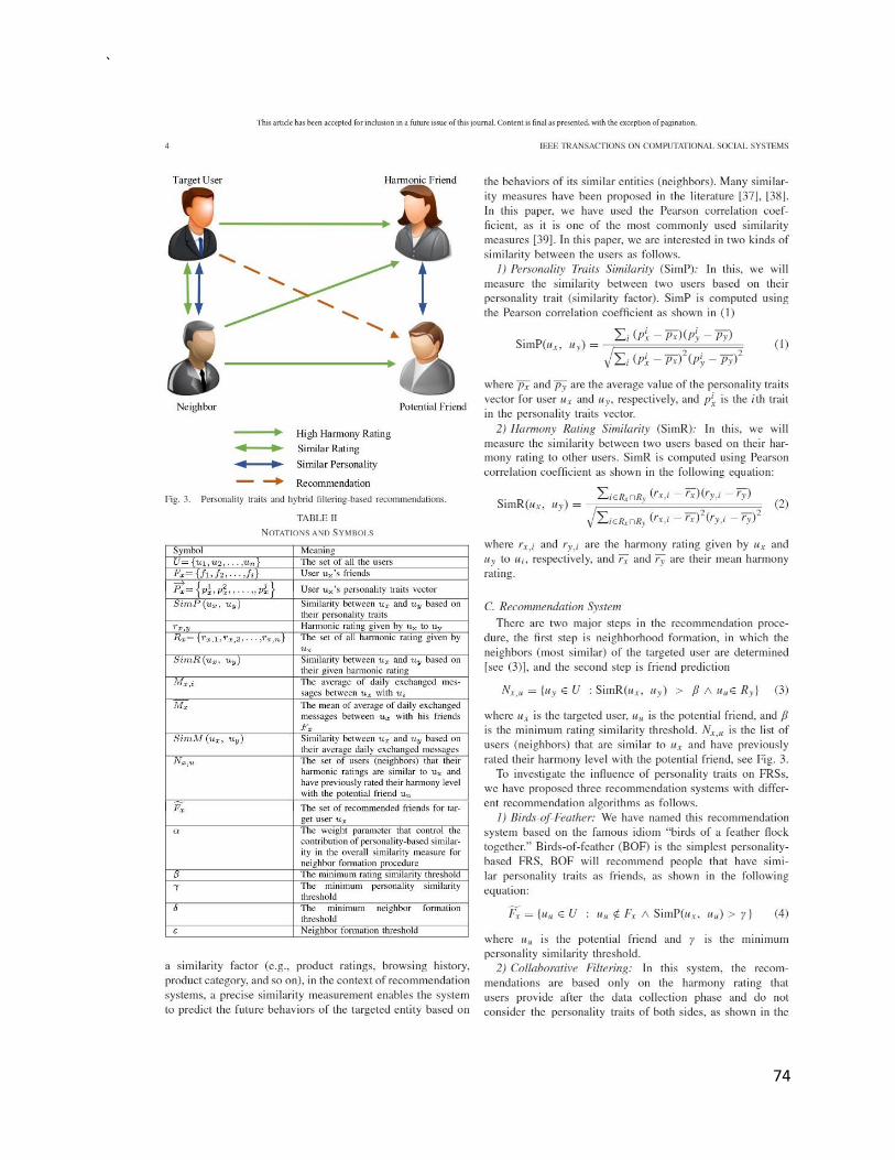
74

`

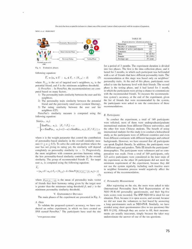
75

`

76

`

77

`

78

`

79

`

80

PUBLISHED PAPER

`

81

`

82

`

83

`

84

`

85

`

86