author's personal copy -...

This article appeared in a journal published by Elsevier. The attachedcopy is furnished to the author for internal non-commercial researchand education use, including for instruction at the authors institution

and sharing with colleagues.

Other uses, including reproduction and distribution, or selling orlicensing copies, or posting to personal, institutional or third party

websites are prohibited.

In most cases authors are permitted to post their version of thearticle (e.g. in Word or Tex form) to their personal website orinstitutional repository. Authors requiring further information

regarding Elsevier’s archiving and manuscript policies areencouraged to visit:

http://www.elsevier.com/copyright

http://www.elsevier.com/copyright

Author's personal copy

Chemical Engineering Science 63 (2008) 5394 -- 5409

Contents lists available at ScienceDirect

Chemical Engineering Science

journal homepage: www.e lsev ier .com/ locate /ces

A two-tier architecture for networked process control

Jinfeng Liua, David Muñoz de la Peñab, Benjamin J. Ohrana, Panagiotis D. Christofidesa,c,∗, James F. Davisa

aDepartment of Chemical and Biomolecular Engineering, University of California, Los Angeles, CA 90095-1592, USAbDepartmento de Ingeniería de Sistemas y Automática, Universidad de Sevilla, Camino de los Descubrimientos S/N, 41092 Sevilla, SpaincDepartment of Electrical Engineering, University of California, Los Angeles, CA 90095-1592, USA

A R T I C L E I N F O A B S T R A C T

Article history:Received 16 May 2008Received in revised form 23 July 2008Accepted 28 July 2008Available online 31 July 2008

Keywords:Nonlinear systemsNetworked control systemsModel predictive controlTime-varying measurement delays

Traditionally, process control systems utilize dedicated, point-to-point wired communication links usinga small number of sensors and actuators to regulate appropriate process variables at desired values.While this paradigm to process control has been successful, chemical plant operation could substantiallybenefit from an efficient integration of the existing, point-to-point control networks (wired connectionsfrom each actuator/sensor to the control system using dedicated local area networks) with additionalnetworked (wired or wireless) actuator/sensor devices. However, augmenting existing control networkswith real-time wired/wireless sensor and actuator networks challenges many of the assumptions made inthe development of traditional process control methods dealing with dynamical systems linked throughideal channels with flawless, continuous communication. In the context of control systems which utilizenetworked sensors and actuators, key issues that need to be carefully handled at the control systemdesign level include data losses due to field interference and time delays due to network traffic. Motivatedby the above technological advances and the lack of methods to design control systems that utilize hy-brid communication networks, in the present work, we present a novel two-tier control architecture fornetworked process control problems that involve nonlinear processes and heterogeneous measurementsconsisting of continuous measurements and asynchronous, delayed measurements. This class of controlproblems arises naturally when nonlinear processes are controlled via control systems based on hybridcommunication networks (i.e., point-to-point wired links integrated with networked wired/wireless com-munication) or utilizing multiple heterogeneous measurements (e.g., temperature measurements whichcan be taken to be continuous and species concentration measurements which are fed to the controlsystem at asynchronous time instants and frequently involve delays). While point-to-point wired linksare very reliable, the presence of a shared communication network in the closed-loop system introducesadditional delays and data losses and these issues should be handled at the controller design level. In thetwo-tier control architecture presented in this work, a lower-tier control system, which relies on point-to-point communication and continuous measurements, is first designed to stabilize the closed-loop system,and an upper-tier networked control system is subsequently designed, using Lyapunov-based model pre-dictive control theory, to profit from both the continuous and the asynchronous, delayed measurementsas well as from additional networked control actuators to improve the closed-loop system performance.The proposed two-tier control architecture preserves the stability properties of the lower-tier controllerwhile improving the closed-loop performance. The applicability and effectiveness of the proposed controlmethod is demonstrated using two chemical process examples.

© 2008 Elsevier Ltd. All rights reserved.

1. Introduction

The chemical industry is a key economic sector in the US and glob-ally, and is involved with the conversion of raw materials, through

* Corresponding author at: Department of Electrical Engineering, Universityof California, Los Angeles, CA 90095-1592, USA. Tel.: +13108252046;fax: +13102064107.

E-mail address: [email protected] (P.D. Christofides).

0009-2509/$ - see front matter © 2008 Elsevier Ltd. All rights reserved.doi:10.1016/j.ces.2008.07.030

a series of chemical processing steps, to valued products. While therange of valuable assets in a chemical plant is large, nearly all theeconomic value in terms of operating profit is a direct result of plantoperations. This realization has motivated extensive research, overthe last 40 years, on the development of advanced operation andcontrol strategies to achieve economically optimal plant operationby regulating process variables at appropriate values. With respectto process control, control systems traditionally utilize dedicated,point-to-point wired communication links using a small number ofsensors and actuators to regulate appropriate process variables at


J. Liu et al. / Chemical Engineering Science 63 (2008) 5394 -- 5409 5395

desired values. While this paradigm to process control has been suc-cessful, chemical plant operation could substantially benefit froman efficient integration of the existing, point-to-point control net-works (wired connections from each actuator/sensor to the controlsystem using dedicated local area networks) with additional net-worked (wired or wireless) actuator/sensor devices (Ydstie, 2002;Davis, 2007; Neumann, 2007; Christofides et al., 2007). Such an augmentation in sensor information and network-based availabilityof wired and wireless data is now well underway in the processindustries and clearly has the potential to be transformative in thesense of dramatically improving the ability of the single-process andplant-wide model-based control systems to optimize process andplant performance. Hybrid communication networks allow for easymodification of the control strategy by rerouting signals, havingredundant systems that can be activated automatically when com-ponent failure occurs, and in general, they allow having a high-level supervisory control over the entire plant (Christofides andEl-Farra, 2005). However, augmenting existing control networkswith real-time wired/wireless sensor and actuator networks chal-lenges many of the assumptions made in the development of tra-ditional process control methods dealing with dynamical systemslinked through ideal channels with flawless, continuous communica-tion. In the context of hybrid communication networks which utilizenetworked sensors and actuators, key issues that need to be care-fully handled at the control system design level include data lossesdue to field interference and time delays due to network traffic.

Motivated by the need to develop control architectures thatutilize hybrid communication networks, we recently introduced atwo-tier control architecture for nonlinear process systems withboth continuous and asynchronous measurements (Liu et al.,submitted for publication). This class of systems arises in the con-text of process control systems utilizing hybrid communicationnetworks consisting of point-to-point wired links integrated withwireless actuator/sensor networks. Assuming that there exists alower-tier control system which relies on point-to-point commu-nication and continuous measurements to stabilize the closed-loopsystem, we proposed to use Lyapunov-based model predictivecontrol (LMPC) theory (Mhaskar et al., 2005, 2006; Muñoz de laPeña and Christofides, 2008) to design an upper-tier networkedcontrol system which profits from both the continuous and theasynchronous measurements as well as from additional networkedcontrol actuators. LMPC is based on the concept of uniting modelpredictive control with control Lyapunov functions as a way ofguaranteeing closed-loop stability. The main idea is to formulateappropriate constraints in the predictive controller's optimizationproblem based on an existing Lyapunov-based controller, in sucha way that the MPC inherits the robustness and stability proper-ties of the Lyapunov-based controller. LMPC schemes allow for anexplicit characterization of the stability region and lead to reducedcomplexity optimization problems. We established in Liu et al.(submitted for publication) that the proposed two-tier control sys-tem architecture preserves the stability properties of the lower-tiercontroller while improving the closed-loop performance. However,the developed two-tier control architecture (Liu et al., submitted forpublication) does not account for the effect of time-varying networkdelays as well as measurement sensor delays, which are particu-larly important during the measurement of species concentrationsand particle size distributions in process control applications. Thus,when time-varying measurement delays are present in the closed-loop system, the developed two-tier control architecture (Liu et al.,submitted for publication) is not guaranteed to maintain the desiredclosed-loop stability and performance properties.

Within process control, other important recent work on the sub-ject of networked process control includes the development of aquasi-decentralized control framework for multi-unit plants that

achieves the desired closed-loop objectives with minimal cross com-munication between the plant units under state (Sun and El-Farra,2008) feedback control. In this work, the key ideas are to embed inthe local control system of each unit a set of dynamic models thatprovide an approximation of the interactions between a given unitand its neighbors in the plant when measurements are not trans-mitted through the plant-wide network and to update the state ofeach model using measurements from the corresponding unit whencommunication is re-established. Using a switched system formula-tion, the maximum allowable update period between the sensors ofeach unit and the local controllers of its neighbors has been explicitlycharacterized. In addition to these works, fault diagnosis and fault-tolerant control methods that account for network-induced mea-surement errors have been developed in Ghantasala and El-Farra(2008). In terms of other research work pertaining to the controlproblem studied in this paper, we note that most of the available re-sults on MPC of systems with delays deal with linear systems (e.g.,Jeong and Park, 2005; Liu et al., 2007). Furthermore, the importanceof time delays in the context of networked control systems has mo-tivated significant research efforts in modeling such delays and de-signing control systems to deal with them, primarily in the contextof linear systems (e.g., Lian et al., 2003; Montestruque and Antsak-lis, 2004; Wang et al., 2005; Zhang et al., 2005; Witrant et al., 2007;Gao et al., 2008). Finally, we recently developed an LMPC techniquefor nonlinear systems with time-varying measurement delays (Liuet al., in press).

In this work, we continue on our recent efforts (Liu et al., sub-mitted for publication) on the development of two-tier control ar-chitectures for networked process control problems. Specifically, wefocus on networked process control problems that involve nonlin-ear processes, hybrid communication networks subjected to datalosses and time delays, and heterogeneous measurements consistingof continuous measurements (e.g., temperature measurements) andasynchronous, delayed measurements (e.g., species concentrationmeasurements which are fed to the control system at asynchronoustime instants and frequently involve delays). We propose a two-tiercontrol architecture which consists of: (a) a lower-tier control sys-tem, which relies on point-to-point communication and continuousmeasurements, to stabilize the closed-loop system, and (b) an upper-tier networked control system, designed using LMPC, that profitsfrom both the continuous and the asynchronous, delayed measure-ments as well as from additional networked control actuators toimprove the closed-loop system performance. The applicability andeffectiveness of the proposed control architecture is demonstratedusing two chemical process examples.

2. Preliminaries

2.1. Problem formulation

In this work, we consider nonlinear process systems describedby the following state-space model:

x(t) = f (x(t),us(t),ud(t),w(t))

ys(t) = hs(x(t))

yd(t) = hd(x(t − d(t))) (1)

where x(t) ∈ Rnx denotes the vector of state variables, ys(t) ∈ Rnysdenotes continuous and synchronous measurements, yd(t) ∈ Rnydare sampled, asynchronous measurements subject to time-varyingmeasurement delays, us(t) ∈ Rnus and ud(t) ∈ Rnud are two dif-ferent sets of possible manipulated inputs, d(t) is the size of thetime-varying measurement delay (see Section 2.2 below for pre-cise definition of the measurement/network model) and w(t) ∈ Rnw

denotes the vector of disturbance variables (i.e., w(t) may include


5396 J. Liu et al. / Chemical Engineering Science 63 (2008) 5394 -- 5409

unknown/partially known time-varying process parameters and/orexternal disturbances). The disturbance vector is assumed to bebounded, i.e., w(t) ∈ W where

W := {w ∈ Rnw s.t. |w|��,� >0}1

We assume that f is a locally Lipschitz vector function, hs and hd aresufficiently smooth vector functions, and f (0, 0, 0, 0)=0, hs(0)=0 andhd(0) = 0. This means that the origin is an equilibrium point for thenominal system (system (1) with w(t) ≡ 0 for all t) with us = 0 andud = 0.

Remark 1. The two sets of inputs include both systemswithmultipleinputs and systems with a single input divided artificially into twoterms; i.e.,

x(t) = f (x(t),u(t),w(t))

with u(t) = us(t) + ud(t)

Remark 2. The set of manipulated inputs ud(t) can be used tomodel actuators controlled via a shared communication network,and hence, possibly affected by data losses or time-varying delays.The set of manipulated inputs us(t) can be used to model controlactuators which are connected with the control system via dedi-cated, wired links and are guided by a control system that only usescontinuous measurements of the outputs ys(t).

2.2. Modeling of measurements/network

System (1) is controlled using both continuous synchronous, ys,and asynchronous, delayed measurements, yd. This class of systemsarises naturally in process control applications, where different pro-cess variables have to be measured such as temperature, flow rates,species concentrations or particle size distributions. This model isalso of interest in the context of processes controlled through a hy-brid communication network in which networked wired/wirelesssensors and actuators are used to add redundancy to existing con-trol loops (which use point-to-point wired communication links andcontinuous measurements) because networked communication isoften subject to data losses due to field interference (for example, inwireless communication) and time-varying delays due to networktraffic. We assume that ys is available for all t, while delayed yd sam-ples are received at an asynchronous rate. We also assume that eachyd measurement is time-labeled, so the controller is able to discardnon-relevant information. Delays in the computation and implemen-tation of control actions can be readily lumped with the measure-ment delays and are not treated separately. The time instants atwhich a new delayed yd sample is received are denoted tk, where{tk�0} is a random increasing sequence of times. To model the time-varying delay, an auxiliary variable dk is introduced to indicate thedelay corresponding to the sample received at time tk; that is, attime instant tk, the sample yd(tk) = hd(x(tk − dk)) is received.

In general, if the sequence {dk�0} is modeled using a randomprocess, there exists the possibility of arbitrarily large delays. In thiscase, it is improper to use all the delayed measurements to estimatethe current state and decide the control inputs, because when thedelays are too large, they may introduce enough errors to destroythe stability of the closed-loop system. In order to study the stabil-ity properties in a deterministic framework, in this paper, we onlytake advantage of delayed measurements such that the delays asso-ciated with the measurements are smaller than an upper bound D,

1 | · | denotes Euclidean norm of a vector.

Process

Sensors

x

Lower-tierController

ys

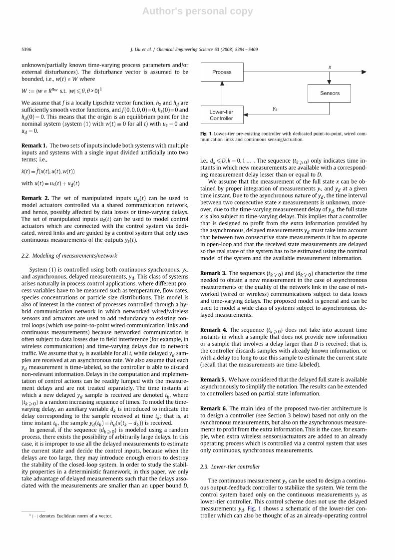
Fig. 1. Lower-tier pre-existing controller with dedicated point-to-point, wired com-munication links and continuous sensing/actuation.

i.e., dk�D, k = 0, 1 . . . . The sequence {tk�0} only indicates time in-stants in which new measurements are available with a correspond-ing measurement delay lesser than or equal to D.

We assume that the measurement of the full state x can be ob-tained by proper integration of measurements ys and yd at a giventime instant. Due to the asynchronous nature of yd, the time intervalbetween two consecutive state x measurements is unknown, more-over, due to the time-varying measurement delay of yd, the full statex is also subject to time-varying delays. This implies that a controllerthat is designed to profit from the extra information provided bythe asynchronous, delayed measurements yd must take into accountthat between two consecutive state measurements it has to operatein open-loop and that the received state measurements are delayedso the real state of the system has to be estimated using the nominalmodel of the system and the available measurement information.

Remark 3. The sequences {tk�0} and {dk�0} characterize the timeneeded to obtain a new measurement in the case of asynchronousmeasurements or the quality of the network link in the case of net-worked (wired or wireless) communications subject to data lossesand time-varying delays. The proposed model is general and can beused to model a wide class of systems subject to asynchronous, de-layed measurements.

Remark 4. The sequence {tk�0} does not take into account timeinstants in which a sample that does not provide new informationor a sample that involves a delay larger than D is received; that is,the controller discards samples with already known information, orwith a delay too long to use this sample to estimate the current state(recall that the measurements are time-labeled).

Remark 5. Wehave considered that the delayed full state is availableasynchronously to simplify the notation. The results can be extendedto controllers based on partial state information.

Remark 6. The main idea of the proposed two-tier architecture isto design a controller (see Section 3 below) based not only on thesynchronous measurements, but also on the asynchronous measure-ments to profit from the extra information. This is the case, for exam-ple, when extra wireless sensors/actuators are added to an alreadyoperating process which is controlled via a control system that usesonly continuous, synchronous measurements.

2.3. Lower-tier controller

The continuous measurement ys can be used to design a continu-ous output-feedback controller to stabilize the system. We term thecontrol system based only on the continuous measurements ys aslower-tier controller. This control scheme does not use the delayedmeasurements yd. Fig. 1 shows a schematic of the lower-tier con-troller which can also be thought of as an already-operating control



system. To proceed, we assume that there exists an output feedbackcontroller us(t) = ks(ys(t)) (where ks(ys) is assumed to be a suffi-ciently smooth function of ys) that renders the origin of the nom-inal closed-loop system (i.e., w(t) ≡ 0) asymptotically stable withud(t) ≡ 0. Using converse Lyapunov theorems (see Khalil, 1996),this assumption implies that there exist functions �i(·), i = 1, 2, 3, 4of class K2 and a Lyapunov function V for the nominal closed-loopsystem which is continuous and bounded in Rnx , that satisfy thefollowing inequalities:

�1(|x|)�V(x)��2(|x|)�V(x)�x

f (x, ks(hs(x)), 0, 0)� − �3(|x|)∣∣∣∣�V(x)�x

∣∣∣∣ ��4(|x|) (2)

for all x ∈ O ⊆ Rnx where O is an open neighborhood of the ori-gin. We denote the region ��3 ⊆ O as the stability region of theclosed-loop system under the controller ks(ys). In the remainder,we will refer to the controller ks as the lower-tier controller. Thelower-tier controller based on the output-feedback controller ks isable to stabilize the system, however, it does not profit from theextra information provided by yd and does not utilize ud(t). In whatfollows, we propose a two-tier control architecture that profitsfrom the extra measurements and control actuators to improve theclosed-loop system performance.

Remark 7. The assumption that there exists a lower-tier controllerwhich can stabilize the closed-loop system using only the continu-ous measurements ys(t) and the inputs us(t) implies that, in princi-ple, it is not necessary to use the additional information providedby the asynchronous measurements and the extra inputs ud(t) inorder to achieve closed-loop stability. However, the main objectiveof the proposed two-tier control architecture is to profit from thisextra information and control effort to improve the closed-loop per-formance while maintaining the stability properties achieved by thelower-tier controller.

Remark 8. We have considered static lower-tier controllers to sim-plify the notation. The formulation can be readily extended to dy-namic lower-tier controllers as long as they enforce asymptotic sta-bility in the closed-loop system in the sense of (2). In the examplesin Sections 4 and 5, proportional-integral (PI) controllers are used asthe lower-tier controllers.

Remark 9. The lower tier controller provides some degree of ro-bustness with respect to the uncertainty w. Condition (2) and theLipschitz property of f guarantee that: (a) the closed-loop nominalsystem under the lower-tier controller is asymptotically stable; (b)the closed-loop system under the lower-tier controller subject to thedisturbances is ultimately bounded, provided � is sufficiently small,in a region that contains the origin that depends on the size of theuncertainty. These properties are made explicit in Proposition 1 innext section. See Khalil (1996) for more details.

3. Two-tier architecture

The main objective of the two-tier control architecture is toimprove the performance of the closed-loop system using the in-formation provided by yd while guaranteeing that the stability

2 Class K functions are strictly increasing functions of their argument andsatisfy �(0) = 0.

3 We use �r to denote the set �r := {x ∈ Rnx |V(x)� r}.

Process

Sensors

x

Lower-tierController

ysyd

Upper-tierController

us

ysyd

ud

Fig. 2. Two-tier control strategy (solid lines denote dedicated point-to-point, wiredcommunication links and continuous sensing/actuation; dashed lines denote net-worked (wired/wireless) communication and/or asynchronous sampling/actuation).

properties of the lower-tier controller are maintained. This is doneby designing a controller (upper-tier controller) based on the fullstate measurements obtained by integrating both the continuousand the asynchronous, delayed measurements. In the two-tier con-trol architecture, the upper-tier controller decides the trajectory ofud(t) between successive samples, i.e., for t ∈ [tk, tk+1] while thelower-tier controller decides us using the continuously availablemeasurements. Fig. 2 shows a schematic of the proposed strategy.The upper-tier controller has to take into account time-varying de-lays and that the time interval between two consecutive samplesis unknown. In the following subsections, we present a two-tier ar-chitecture based on LMPC theory for the design of the upper-tiercontroller, which maintains the stability properties of the lower-tier controller while improving the closed-loop performance.

Remark 10. Note that since the lower-tier controller has alreadybeen designed, this controller views the input ud as a disturbancethat has to be rejected if the controller that manipulates ud is notproperly designed. Therefore, the design of the upper-tier controllerhas to take into account the decisions that will be made by thelower-tier controller to maintain closed-loop stability and improvethe closed-loop performance.

3.1. Upper-tier LMPC design

In order to take advantage of the model of the system and theasynchronous, delayed measurements yd, we propose to use LMPCtheory to decide ud. The main idea of the proposed model predictivecontroller is the following: at each time instant tk when a new asyn-chronous measurement yd(tk) is received, a delayed state measure-ment x(tk−dk) is obtained by integrating this measurement with thepreviously received synchronous measurement ys(tk −dk). Based onthis delayed state measurement x(tk −dk), the nominal model of thesystem, the continuous measurements ys(t) and the control inputsapplied from tk − dk to tk, an estimate of the current state x(tk) iscomputed. Note that this implies that the upper-tier controller has tostore its past control input trajectory, know the explicit expressionand parameters of the lower-tier controller and use the continuousmeasurements ys(t) to predict the control inputs carried out by thelower-tier controller. The estimated state x(tk) is then used to ob-tain the optimal future control input trajectory ud = u∗

d,k by meansof an LMPC optimization problem. This input trajectory is imple-mented until a new measurement arrives at time tk+1. If the timebetween two consecutive measurements is longer than the predic-tion horizon, ud is set to zero until a new measurement arrives andthe optimal control problem is solved again.

In order to define a finite dimensional optimization problem, ud isconstrained to belong to the family of piece-wise constant functionswith sampling period �, S(�). To guarantee that the resulting closed-loop system is stable, we follow an LMPC approach for the design of



the upper-tier controller, see Mhaskar et al. (2005, 2006) and Muñozde la Peña and Christofides (2008). LMPC is based on including acontractive constraint that allows to prove practical stability of theclosed-loop system using an auxiliary Lyapunov-based controller. Inthe previous LMPC schemes (Mhaskar et al., 2005, 2006; Muñoz de laPeña and Christofides, 2008), the contractive constraints are definedbased on a known Lyapunov-based state feedback controller. In thepresent work, the contractive constraint of the proposed upper-tierLMPC design is based on the Lyapunov function of the closed-loopsystem under the lower-tier controller ks. Specifically, the upper-tierLMPC optimization problem is defined as follows:

u∗d,k(t) = arg min

ud,k∈S(�)

∫ tk+�f

tk−dkL(x(�), ks(hs(x(�))),ud,k(�)) d� (3a)

˙x(t) = f (x(t), ks(hs(x(t))),ud,k(t), 0), ∀t ∈ [tk − dk, tk) (3b)

˙x(t) = f (x(t), ks(hs(x(t))),ud,k(t), 0), ∀t ∈ [tk, tk + �f ] (3c)

x(tk − dk) = x(tk − dk) (3d)

ud,k(t) = u∗d,k−1(t), ∀t ∈ [tk − dk, tk] (3e)

˙x(t) = f (x(t), ks(hs(x(t))), 0, 0), t ∈ [tk, tk + �f ] (3f)

x(tk) = x(tk) (3g)

V(x(t))�V(x(t)), ∀t ∈ [tk, tk + �f ] (3h)

where x(tk − dk) is the state obtained integrating both the measure-ments of ys(tk − dk) and yd(tk) = hd(x(tk − dk)), x(t) is the predictedtrajectory of the two-tier nominal system for the input trajectorycomputed by the LMPC, x(t) is the predicted trajectory of the two-tier nominal system for the input trajectory ud(t) ≡ 0 for all t ∈[tk, tk + �f ], L(x,us,ud) is a positive definite function of the state andthe inputs that define the cost, and �f is the prediction horizon. Thisoptimization problem does not depend on the uncertainty and as-sures that the system in closed-loop with the upper-tier controllermaintains the stability properties of the lower-tier controller. Theoptimal solution to this optimization problem is denoted by u∗

d,k(t).This signal is defined for all t > tk with u∗

d,k(t) = 0 for all t > tk + �f .The control inputs of the proposed two-tier control architecture

based on the above LMPC are defined as follows:

us(t) = ks(hs(x(t))), ∀tud(t) = u∗

d,k(t), ∀t ∈ [tk, tk+1) (4)

where u∗d,k(t) is the optimal solution to the LMPC problem at time

step tk. This implementation technique takes into account that thelower-tier controller uses the continuously available measurements,while the upper-tier controller has to operate in open-loop betweenconsecutive asynchronous, delayed measurements.

Remark 11. Note that by definition, u∗d,k(t) is defined for all t > tk

with u∗d,k(t)=0 for all t > �f . This implies that the upper-tier controller

switches off when it has been operating in open-loop for a largetime, because in this case, the last received information is no longeruseful to improve the performance of the lower-tier controller. Fur-thermore, we note that the extension of the LMPC scheme of Eq. (3)to the case where the upper-tier controller receives the ys measure-ments asynchronously subject to delays is conceptually straightfor-ward.

Remark 12. In the proposed LMPC optimization problem both theestimation of x(tk) from x(tk − dk) and the evaluation of the fu-ture optimal input trajectory in [tk, tk+1] are carried out at the sametime. First, the constraints of the problem guarantee that x(tk) has

been estimated using the nominal model (constraint (3b)) and thereal inputs applied to the system (constraint (3e)) from the initialstate x(tk −dk) (constraint (3d)). Once the current state is estimated,the future input trajectory is optimized to minimize the cost func-tion taking into account the lower-tier controller (constraint (3c))while guaranteeing that the contractive constraint is satisfied (con-straint (3h)). This optimization problem has been proposed in orderto present a compact controller formulation. It is possible to decou-ple the observer and the LMPC optimization problem as long as theobserver provides an upper bound on the estimation error of x(tk).For example, a high-gain observer can be used to estimate x(tk) fromthe continuous measurements and the applied inputs, and then usethis estimated state to define the LMPC optimization problem.

Remark 13. Constraints (3c) and (3h) are a key element of theproposed two-tier control architecture. In general, guaranteeingclosed-loop stability of a distributed control scheme is a difficulttask because of the interactions between the different controllersand can only be done under certain assumptions (see, for example,Rawlings and Stewart, 2007; Camponogara et al., 2002). Constraint(3c) guarantees that the upper-tier controller takes into accountthe effect of the lower-tier controller to the applied inputs (recallthat the lower-tier controller is designed without taking ud intoaccount). Constraint (3h) will be used to guarantee that the valueof the Lyapunov function is a decreasing sequence of time with alower bound.

3.2. Two-tier controller stability

Using asynchronous and delayed measurements without propercare in the control systemmay deteriorate the stability of the closed-loop system. In order to maintain the closed-loop system stabil-ity properties enforced by the lower-tier controller and improvethe performance of the closed-loop system, we propose to followa Lyapunov-based approach. The main idea, is to compute the in-put ud applied to the system in a way such that it is guaranteedthat in the closed-loop system the value of the Lyapunov function attime instants tk; that is, V(x(tk)), is a decreasing sequence of valueswith a lower bound. Following Lyapunov-like arguments, this prop-erty guarantees practical stability of the closed-loop system. This isachieved thanks to the contractive constraint of the LMPC optimiza-tion problem (3). This property is presented in Theorem 1 below. Tostate and prove this theorem, we need to state the following threepropositions:

Proposition 1 (cf. Khalil, 1996). Consider system (1) in closed-loopwith the lower-tier controller. Taking into account (2), there exists aKL4 function �, a K function and a constant �max such that ifx(0) ∈ �� and ud(t) ≡ 0 then

V(x(t))��(V(x(t0)), t − t0) +

(max

�∈[t0,t]|w(�)|

)

for all w ∈ W with ��max.

This proposition provides us with a bound on the trajectories ofthe Lyapunov function of the state of the system in closed-loop underthe lower-tier controller with ud(t) ≡ 0. We will use this bound toprove the stability theorem. The proof of Proposition 1 can be foundin Khalil (1996).

4 Function �(r, s) is said to be a class KL function if, for each fixed s, �(r, s)belongs to classK function with respect to r and, for each fixed r, �(r, s) is decreasingwith respect to s and �(r, s) → 0 as s → 0.



Proposition 2. Consider the following state trajectories:

xa(t) = f (xa(t), ks(hs(xa(t))),ud(t),w(t))

xb(t) = f (xb(t), ks(hs(xb(t))),ud(t), 0) (5)

with initial states xa(t0)= xb(t0) ∈ ��. There exists a class K functionfW (s) such that

|xa(t) − xb(t)|� fW (t − t0) (6)

for all xa(t), xb(t) ∈ �� and all w(t) ∈ W .

Proof. Define the error vector as e(t)=xa(t)−xb(t). The time deriva-tive of the error is given by

e(t) = f (xa(t), ks(hs(xa(t))),ud(t), 0) − f (xb(t), ks(hs(xb(t))),ud(t), 0)

By continuity and the local Lipschitz property assumed for the vectorfield f (x,us,ud,w), there exist positive constants Lw, Lx and Lu1 suchthat

|e(t)|�Lw|w(t) − 0| + Lx|xa(t) − xb(t)|+ Lu1|ks(hs(xa(t))) − ks(hs(xb(t)))| (7)

for all xa(t), xb(t) ∈ �� andw(t) ∈ W . By continuity and local Lipschitzproperty of ks and hs, there exists a positive constant Lu2 such that

|ks(hs(xa(t))) − ks(hs(xb(t)))|�Lu2|xa(t) − xb(t)|

Thus, the following inequality can be obtained from inequality (7):

|e(t)|�Lw|w(t) − 0| + Lx|xa(t) − xb(t)| + Lu1Lu2|xa(t) − xb(t)|� Lw� + (Lx + Lu1Lu2)|e(t)|

Integrating |e(t)| with initial condition e(t0)=0 (recall that xa(t0)=xb(t0)), the following bound on the norm of the error vector is ob-tained:

|e(t)|� Lw�L′x

(eL′x(t−t0) − 1)

where L′x = Lx + Lu1Lu2. This implies that Eq. (6) holds for

fW (�) = Lw�L′x

(eL′x� − 1) �

The following proposition bounds the difference between themagnitudes of the Lyapunov function of two different states in ��.

Proposition 3. Consider the Lyapunov function V(·) of system (1). Thereexists a quadratic function fV (·) such that

V(x)�V(x) + fV (|x − x|) (8)

for all x, x ∈ ��.

Proof. Because the Lyapunov function V(x) is continuous andbounded on compact sets, we can find a positive constant M suchthat a Taylor series expansion of V around x yields

V(x)�V(x) + �V�x

|x − x| + M|x − x|2, ∀x, x ∈ ��

Note that the term M|x − x|2 bounds the high order terms of theTaylor series of V(x) for all x, x ∈ ��. Taking into account Eq. (2), thefollowing bound for V(x) is obtained:

V(x)�V(x) + �4(�−11 (�))|x − x| + M|x − x|2, ∀x, x ∈ ��

This implies that Eq. (8) holds for fV (x) = �4(�−11 (�))x + Mx2. �

ttk − D tk tk + τf tk+1

x (t)

x (t)

x (t)x (t)

˜

Fig. 3. Possible worst scenario of the delayed measurements received by the up-per-tier controller and the corresponding state trajectories defined in problem (3).

We are now in a position to state and prove the main stabilityresult for the proposed two-tier control architecture.

Theorem 1. Consider system (1) in closed-loop with the two-tier con-trol architecture (4). If x(t0) ∈ ��, ��max, and there exist a concavefunction g such that

g(x)��(x + fV (fW (D)), �f )

for all x ∈ ��, and a positive constant c�� such that

c − g(c)� fV (fW (D + �f )) (9)

then x(t) is ultimately bounded in a region that contains the origin.

Proof. In order to prove that system (1) in closed-loop under thetwo-tier control architecture using the proposed LMPC (3) is ulti-mately bounded in a region that contains the origin, we will provethat the value of the Lyapunov function at times {tk�0}, V(x), is adecreasing sequence of values with a lower bound on its magnitudefor the worst possible case from the communications point of view,and hence for all possible sequences of measurement times and de-lays. The worst possible case from the communications point of viewis that the measurements used to evaluate the upper-tier LMPC con-troller are always received with the maximum delay D; that is dk=Dfor all k, and that the upper-tier controller always operates in open-loop for a period of time longer than �f between consecutive sam-pling times, that is, tk+1 − tk > �f for all k. If the measurements arereceived with a smaller delay or more often, the LMPC has moreprecise information of the state of the system.

Fig. 3 shows the worst scenario for a system of dimension 1. Solidvertical lines are used to indicate the times at which new measure-ments are obtained (tk and tk+1) and when the upper-tier controllerswitches off at time tk+�f . The dashed vertical line indicates the timecorresponding to the measurement obtained at tk (that is, tk − D).In this figure, three different state trajectories are shown. The realstate trajectory of system (1) (including the uncertainty) is denotedas x(t). The estimated state trajectory from tk −D to tk and the pre-dicted sampled trajectory under the two-tier control architecturecomputed by the LMPC (3) along the prediction horizon with initialstate the estimated state are denoted as x(t). The nominal trajectoryunder the lower-tier controller ks with ud ≡ 0 along the predictionhorizon with initial state the estimated state x(tk) is denoted as x(t).The state trajectories x(t) and x(t) are obtained using the two-tiernominal model as defined in the LMPC optimization problem (3).

The trajectory x(t) corresponds to the nominal system in closed-loop with the lower-tier controller with initial state x(tk). Taking intoaccount Proposition 1 the following inequality holds:

V(x(t))��(V(x(tk)), t − tk) (10)



The contractive constraint of the proposed LMPC guarantees that

V(x(t))�V(x(t)), ∀t ∈ [tk, tk + �f ] (11)

Taking into account constraints (3b)–(3d) and that the closed-looptrajectories are defined by the following equation:

x(t) = f (x(t), ks(hs(x(t))),ud,k(t),w(t))

we can apply Proposition 2 to obtain the following upper bounds onthe deviation of x(t) from x(t)5 :

|x(tk) − x(tk)|� fW (D)

|x(tk + �f ) − x(tk + �f )|� fW (�f + D)

From Proposition 3 and the above inequalities, we obtain the follow-ing inequalities:

V(x(tk))�V(x(tk)) + fV (fW (D))

V(x(tk + �f ))�V(x(tk + �f )) + fV (fW (D + �f )) (12)

From inequalities (10)–(12), the following upper bound on V(x(tk +�f )) is obtained:

V(x(tk + �f ))��(V(x(tk)) + fV (fW (D)), �f ) + fV (fW (D + �f )) (13)

Taking into account that for all t > tk + �f the upper-tier controlleris switched off, i.e., ud(t) = 0, and only the lower-tier controlleris in action, the following bound on V(x(tk+1)) is obtained fromProposition 1:

V(x(tk+1))� max{V(x(tk + �f )), (�max)}for allw(t) ∈ W . Because function g is concave, z−g(z) is an increasingfunction. If there is a constant c0�c�� satisfying Eq. (9), then Eq. (9)holds for all z > c. Taking into account that g(z)��(z + fV (fW (D)), �f )for all z��, the following inequality is obtained:

z − �(z + fV (fW (D)), �f )� fV (fW (D + �f ))

when c�z��. From this inequality and inequality (13), we obtainthat

V(x(tk+1))� max{V(x(tk)), (�max)}for all V(x(tk))�c. It follows using Lyapunov arguments that

lim supt→∞

V(x(t))��c

where

�c = max{maxc

�(c + fV (fW (D)), �f )

+fV (fW (D + �f )), (�max)}. �

Remark 14. In general the size of the region in which the state isultimately bounded, depends on the maximum delay D and the pre-diction horizon �f . The upper bound on delay D sets the largest sizeof delay allowed in the measurements used to evaluate the upper-tier controller and the prediction horizon �f sets the maximumamount of time inwhich the upper-tier controller will be operating inopen-loop.

5 Proposition 2 is used to obtain a bound on the difference between x and xfrom tk −dk to tk to simplify the notation and the proof. Note that from tk −dk to tk ,the real trajectory of us is applied to evaluate x, so tighter bound on the differencebetween x and x can be obtained. As mentioned before, the estimation of x(tk) canbe done using any observer which provides a bound on the estimation error.

Remark 15. Referring to Theorem 1, the assumption that there existsa concave function g such that g(x)��(x + fV (fW (D)), �f ) for all x ∈�� imposes upper bounds on D and �f and is made, without anyloss of generality, to simplify the proof of Theorem 1; i.e., the resultof Theorem 1 could still be proved without this assumption but theproof would be more involved. The assumption that there exists apositive constant c�� such that c− g(c)� fV (fW (D+ �f )) guaranteesthat the derivative of the Lyapunov function of the state of the closed-loop system outside the level set V(x)= c is negative under the two-tier control architecture with the upper-tier LMPC (3).

Remark 16. Although the proofs provided are constructive, the con-stants obtained are conservative. This is the case with most of theresults of the type presented in the literature, see for example Ne�si �cet al. (1999) and Tabuada and Wang (2006) for further discussion onthis issue. In practice, the maximum time that the system can oper-ate in open-loop is better estimated through closed-loop simulation.The various inequalities proved in this theorem are more useful asguidelines on the interaction between the various parameters thatdefine the system and the controller and may be used as guidelinesto design the controller.

4. Application to a chemical reactor

4.1. Process description and modeling

Consider a well mixed, non-isothermal continuous stirred tankreactor (CSTR) where three parallel irreversible elementary exother-mic reactions take place of the form A → B, A → C and A → D. Prod-uct B is the desired product and C and D are byproducts. The feedto the reactor consists of A at temperature TA0 and concentrationCA0 and flow rate F + �F, where �F is a time-varying uncertainty.Due to the non-isothermal nature of the reactor, a jacket is used toremove/provide heat from/to the reactor. Using first principles andstandard modeling assumptions, the following mathematical modelof the process is obtained:

dTdt

= F + �FVr

(TA0 − T) −3∑

i=1

�Hicp

ki0 e−Ei/RTCA + Q

cpVr

dCAdt

= F + �FVr

(CA0 − CA + �CA0) +3∑

i=1

ki0 e−Ei/RTCA (14)

where CA denotes the concentration of the reactant A, T denotes thetemperature of the reactor, Vr denotes the volume of the reactor,�Hi, ki0 and Ei, i=1, 2, 3 denote the enthalpies, pre-exponential con-stants and activation energies of the three reactions, respectively,and cp and denote the heat capacity and the density of the fluidin the reactor, respectively. The inputs to the system are the rate ofheat input/removal Q and the change of the inlet reactant A concen-tration �CA0. The values of the process parameters are presented inTable 1.

System (14) has three steady-states (two locally asymptoticallystable and one unstable). The control objective is to stabilize the sys-tem at the open-loop unstable steady-state Ts=388K, CAs=3.59mol/l.The flow rate uncertainty is bounded by |�F|�4m3/h.

The process model (14) belongs to the class of nonlinear systemsdescribed by system (1) where xT = [x1 x2]= [T − Ts CA − CAs] is thestate, us = Q and ud = �CA0 are the manipulated inputs, � = �F is atime varying bounded disturbance, ys = x1 = T − Ts is obtained fromthe continuous temperature measurements T and yd = x2 = CA − CAsis obtained at time instants {tk�0} from the asynchronously sam-pled concentration measurement CA subject to time-varying mea-surement delays. We also have a lower bound Tmin = 0.15h onthe time interval between two consecutive concentration measure-ments and an upper bound D on the size of the delay; both will be



Table 1Process parameters

F 4.998m3/hVr 1m3

R 8.314KJ/kmolKTA0 300KCA0s 4kmol/m3

�H1 −5.0 × 104 KJ/kmol�H2 −5.2 × 104 KJ/kmol�H3 −5.4 × 104 KJ/kmolk10 3 × 106 h−1

k20 3 × 105 h−1

k30 3 × 105 h−1

E1 5 × 104 KJ/kmolE2 7.53 × 104 KJ/kmolE3 7.53 × 104 KJ/kmol 1000kg/m3

cp 0.231KJ/kgK

computed via simulations even though conservative estimates couldbe computed from the theoretical results.

To model the time sequence {tk�0}, we use a lower-boundedrandom Poisson process. The Poisson process is defined by the num-ber of events per unit time W. The interval between two consecu-tive concentration sampling times (events of the Poisson process)is given by �a = max{Tmin,− ln�/W}, where � is a random variablewith uniform probability distribution between 0 and 1. In order tomodel the delay size sequence {dk�0}, the size of delay associatedwith the concentration measurement at tk is modeled by an upper-bounded random process given by dk=min{D,�L}, where � is a uni-formly distributed variable between 0 and 1, and L= tk − tk−1 +dk−1is the size of the time interval between current time tk and the timecorresponding to the last concentration measurement tk−1 − dk−1.This generation method guarantees that dk�D for all k. We assumethat the initial state is known; that is, d0 = 0 and t0 = 0.

4.2. Lower-tier controller design

An output feedback controller (lower-tier controller) based on thecontinuous temperature measurements (i.e., x1(t)) is first designedto stabilize system (14) using only the rate of heat input us = Q asthe manipulated input. In particular, the following PI control law isused as the lower-tier controller:

us(t) = K

(x1(t) + 1

Ti

∫ t

0x1(�) d�

)(15)

where K is the proportional gain and Ti is the integral time constant.To compute the parameters of the PI controller, the linearized modelx=Ax+Bus of system (14) around the equilibrium point is obtained.The proportional gain K is chosen to be −8100. This value guaranteesthat the origin of x = (A + BK[1 0])x is asymptotically stable withits eigenvalues being 1 = −1.06 × 105 and 2 = −4.43. A quadraticLyapunov function V(x) = xTPx with

P =[0.024 5.21

5.21 1.13 × 103

]

is obtained by solving an algebraic Lyapunov equation ATc P + PAc +Qc=0 for Pwith Ac=A+BK[1 0]. This Lyapunov function will be usedto design the upper-tier LMPC controller. The integral time constantis chosen to be Ti = 49.6h. For simplicity, the Lyapunov functionV(x) is determined on the basis of the closed-loop system underonly the proportional (P) term of the PI controller; the effect of theintegral (I) term is very small for the specific choice of the controllerparameters used in the simulations and does not change the localstability property of the equilibrium point of the closed-loop systemenforced by the proportional part of the PI controller.

0 0.1 0.2 0.3 0.4 0.5370

380

390

T

0 0.1 0.2 0.3 0.4 0.53.4

3.6

3.8

CA

0 0.1 0.2 0.3 0.4 0.5−1012

x 105

u s0 0.1 0.2 0.3 0.4 0.5

−1

0

1

Time (hr)

u d

Fig. 4. State and input trajectories of system (14) under lower-tier PI control (15)(ud ≡ 0).

The state and input trajectories of system (14) starting from x0 =[370 3.41]T under the PI controller are shown in Fig. 4. From Fig. 4,we see that the PI controller (15) drives the temperature and con-centration states of system (14) close to the equilibrium point inabout 0.1 and 0.2h, respectively.

4.3. Two-tier control architecture design

We have implemented the proposed two-tier control architec-ture to improve the performance of the closed-loop system obtainedunder PI-only control. In this set of simulations, the PI controller (15)with the same parameters is used as the lower-tier controller. In-stead of abandoning the less frequent concentration measurements,we take advantage of both the continuous measurements of the tem-perature, T, and the asynchronous, delayed measurements of theconcentration, CA, together with the nominal model of system (14)to design and implement the upper-tier LMPC. The inlet concentra-tion change �CA0 is the manipulated input for the LMPC.

The LMPC is designed next. The performance index is defined bythe following positive definite function:

L(x,us,ud) = xTQcx (16)

where x is the state of the system and Qc is the following weightmatrix:

Qc =[1 0

0 104

]

The values of the weights in Qc have been chosen to account forthe different range of numerical values for each state. The samplingtime of the LMPC is � = 0.025h; the prediction horizon is chosen tobe �f =6� so that the prediction captures most of the dynamic evo-lution of the process; the quadratic control Lyapunov function V(x)is used in the design of the contractive constraint (3h) and the inletconcentration change �CA0 is bounded by |ud|=|�CA0|�1kmol/m3.



0 0.1 0.2 0.3 0.4 0.5370

380

390

T

0 0.1 0.2 0.3 0.4 0.53.4

3.6

3.8

CA

0 0.1 0.2 0.3 0.4 0.5−1

01

x 105

u s

0 0.1 0.2 0.3 0.4 0.5−1

0

1

u d

Time (hr)

Fig. 5. Worst case state and input trajectories of system (14) under the proposedtwo-tier control architecture.

For the simulations carried out in this subsection, we pick thedelay of each measurement to be dk = D = 0.15h for all k. Thesesettings correspond to the worst-case effect from a communicationpoint of view. Note that the minimum time interval between twoconsecutive concentrationmeasurements Tmin is fixed by the systemdynamics and the prediction horizon is set be equal to the minimumtime interval between two consecutive yd measurements, that is�f = Tmin.

The two-tier control architecture is implemented as discussed inthe previous section. The lower-tier controller uses the continuoustemperature measurements to decide us(t). When a new measure-ment of CA is obtained at time instant tk with delay D, an estimateof the state of system (14), x(tk − D), is obtained by integrating theconcentration measurement and the previously received continuousmeasurement of the temperature T. Based on the state x(tk −D), themodel of the process and the control actions applied, an estimateof the current state x(tk) is obtained. Based on this state estimatex(tk), the LMPC optimization problem (3) is solved and an optimalinput trajectory u∗

d,k(�) is obtained. This optimal input trajectory isimplemented until a new concentration measurement is obtainedat time tk+1 (note that k indexes the number of concentration sam-ples received, not a given sampling time). Note that because a PIcontroller is used in the lower-tier, we need to incorporate the PIcontroller dynamics in the optimization problem of the proposedLMPC scheme (3).

A simulation of the closed-loop system under the two-tier controlarchitecture (4) with the same initial conditions x(0) = [370 3.41]T

has been carried out. The sampling sequence {tk�0} generated withW = 1 and delay size sequence {dk�0} with simulation length of0.5h are the following:

{tk�0} = {0 0.198 0.395 0.500}h

{dk�0} = {0 0.150 0.150 0.150}h

The state and input trajectories of system (14) under the proposedtwo-tier control architecture are shown in Fig. 5. From Fig. 5, we seethat the two-tier control architecture (4) stabilizes the temperature

Table 2Total performance cost along the closed-loop system trajectories

Sim. Two-tier PI control

1 107.60 557.062 124.98 1090.293 188.53 1392.734 169.06 403.825 143.07 376.156 179.22 1330.257 202.28 1252.368 152.23 749.939 141.84 732.20

10 157.99 1049.38

and concentration of the system at the desired equilibrium pointin about 0.1 and 0.05h, respectively. This implies that the resultingclosed-loop system response is faster for this particular simulation.Moreover, the cost associatedwith the resulting closed-loop trajecto-ries is lower. This result has been validated by extensive simulations.

Remark 17. We considered a performance index L(x,us,ud) that pe-nalizes only the closed-loop system state and not the control actionbecause the two-tier control architecture utilizes different manipu-lated inputs from the lower-tier PI controller and this would com-plicate the comparison if penalty on the control action is includedin the cost. Since the performance index has only penalty on theclosed-loop system state, we have included an input constraint onthe upper-tier manipulated input, �CA0, to avoid computation ofunnecessarily large control actions by the upper-tier controller (i.e.,|ud|�1kmol/m3).

4.4. Performance comparison

We also carried out a set of simulations to compare the proposedtwo-tier control architecture with the lower-tier PI control systemfrom a performance index point of view. Table 2 presents the totalcost computed for 20 different closed-loop simulations under theproposed two-tier control architecture and the PI control scheme.To carry out this comparison, we have computed the total cost ofeach simulation based on the integral of the performance index de-fined by L(x,us,ud) of Eq. (16) from the initial time to the end ofthe simulation tf = 0.5h. For each pair of simulations (one for eachcontrol scheme) a different initial state inside the stability region, adifferent uncertainty trajectory and a different random concentra-tion measurement sequence with random delay size sequence aregenerated using the methods described in Section 4.1. As it can beseen in Table 2, the proposed two-tier control architecture has a costlesser than the corresponding total cost under the PI controller in allthe closed-loop system simulations.

Remark 18. Note that in this particular example, the improvementin the closed-loop performance is achieved due to the extra controlinput ud which is guided by the LMPC scheme (3) that uses all avail-able measurements. Since PI controller is used as the lower-tier con-troller, the extra available asynchronous measurements would nothave changed the closed-loop performance achieved by the lower-tier controller because the PI controller cannot use the extra mea-surements. This is also the case for the next example.

5. Application to a reactor–separator process

5.1. Process description and modeling

The process considered in this example is a three vessel,reactor–separator system consisting of two CSTRs and a flash tankseparator (see Fig. 6). A feed stream to the first CSTR F10 containsthe reactant A which is converted into the desired product B. The



F10 F1 F2

F3

Fr Fp

F20

A B C A B C

Fig. 6. Reactor-separator system with recycle.

desired product B can then further react to form an undesiredside-product C. The effluent of the first CSTR along with additionalfresh feed F20 makes up the inlet to the second CSTR. The reactionsA → B and B → C (referred to as 1 and 2, respectively) take placein the two CSTRs in series before the effluent from CSTR 2 is fed toa flash tank. The overhead vapor from the flash tank is condensedand recycled to the first CSTR, and the bottom product stream isremoved. A small portion of the overhead is purged before beingrecycled to the first CSTR. All the three vessels are assumed to havestatic holdup. The dynamic equations describing the behavior ofthe system, obtained through material and energy balances understandard modeling assumptions, are given as follows:

dxA1dt

= F10V1

(xA10 − xA1) + FrV1

(xAr − xA1) − k1 e−E1/RT1xA1

dxB1dt

= F10V1

(xB10 − xB1) + FrV1

(xBr − xB1)

+ k1 e−E1/RT1xA1 − k2 e

−E2/RT1xB1

dT1dt

= F10V1

(T10 − T1) + FrV1

(T3 − T1)

+ −�H1Cp

k1 e−E1/RT1xA1 + −�H2

Cpk2 e

−E2/RT1xB1

+ Q1�CpV1

dxA2dt

= F1V2

(xA1 − xA2) + F20V2

(xA20 − xA2) − k1 e−E1/RT2xA2

dxB2dt

= F1V2

(xB1 − xB2) + F20V2

(xB20 − xB2)

+ k1 e−E1/RT2xA2 − k2 e

−E2/RT2xB2

dT2dt

= F1V2

(T1 − T2) + F20V2

(T20 − T2)

+ −�H1Cp

k1 e−E1/RT2xA2 + −�H2

Cpk2 e

−E2/RT2xB2

+ Q2�CpV2

dxA3dt

= F2V3

(xA2 − xA3) − Fr + FpV3

(xAr − xA3)

dxB3dt

= F2V3

(xB2 − xB3) − Fr + FpV3

(xBr − xB3)

Table 3Process variables

xA1, xA2, xA3 Mass fractions of A in vessels 1–3xB1, xB2, xB3 Mass fractions of B in vessels 1–3xC1, xC2, xC3 Mass fractions of C in vessels 1–3xAr , xBr , xCr Mass fractions of A–C in the recycle streamT1, T2, T3 Temperatures in vessels 1–3T10, T20 Feed stream temperatures to vessels 1 and 2F1, F2 Effluent flow rate from vessels 1 and 2F10, F20 Steady-state feed stream flow rates to vessels 1 and 2Fr , Fp Flow rates of the recycle and purge streamsV1, V2, V3 Volumes of vessels 1–3E1, E2 Activation energy for reactions (1) and (2)k1, k2 Pre-exponential values for reactions (1) and (2)�H1, �H2 Heats of reaction for reactions (1) and (2)�A , �B , �C Relative volatilities of A–CQ1, Q2, Q3 Heat inputs into vessels 1–3Cp , R, � Heat capacity, gas constant and solution density

Table 4Process parameters

T10 300KT20 300KF10 5.04m3/hFr 50.4m3/hFp 5.04m3/hV1 1.0m3

V2 0.5m3

V3 1.0m3

E1 5 × 104 KJ/kmolE2 6 × 104 KJ/kmolk1 2.77 × 103 s−1

k2 2.5 × 103 s−1

�H1 −6 × 104 KJ/kmol�H2 −7 × 104 KJ/kmol�A 3.5�B 1�C 0.5Cp 4.2KJ/kgKR 8.314KJ/kmolK� 1000kg/m3

dT3dt

= F2V3

(T2 − T3) + Q3�CpV3

(17)

where the definitions for the variables can be found in Table 3, withthe parameter values given in Table 4. The model of the flash tankseparator operates under the assumption that the relative volatilityfor each of the species remains constant within the operating tem-perature range of the flash tank. This assumption allows calculatingthe mass fractions in the overhead based upon the mass fractions inthe liquid portion of the vessel. It has also been assumed that thereis a negligible amount of reaction taking place in the separator. Thefollowing algebraic equations model the composition of the over-head stream relative to the composition of the liquid holdup in theflash tank:

xAr = �AxA3�AxA3 + �BxB3 + �CxC3

xBr = �BxB3�AxA3 + �BxB3 + �CxC3

xCr = �CxC3�AxA3 + �BxB3 + �CxC3

(18)

Each of the tanks has an external heat input. The manipulatedinputs to the system are the heat inputs to the three vessels,Q1,Q2 and Q3, and the feed stream flow rate to vessel 2, F20.

System (17) was numerically simulated using a standard Eulerintegration method. The system was modeled with process noise.



Table 5Noise parameters

p � �p

xA1 1 0.7 2xB1 1 0.7 2T1 10 0.7 20xA2 1 0.7 2xB2 1 0.7 2T2 10 0.7 20xA3 1 0.7 2xB3 1 0.7 2T3 10 0.7 20

Table 6Steady-state values of manipulated inputs

Parameters Values

Q1s 12.6 × 105 KJ/hQ2s 16.2 × 105 KJ/hQ3s 12.6 × 105 KJ/hF20s 5.04m3/h

Process noise was added to the right-hand side of each equation inthe system of ODEs found in Eq. (17) and generated as autocorre-lated noise of the form wk = �wk−1 + �k where k = 0, 1, . . . is thediscrete time step of 0.001h, �k is generated by a normally dis-tributed random variable with standard deviation p and � is theautocorrelation factor and wk is bounded by �p, that is |wk|��p.Table 5 contains the parameters used in generating the processnoise.

We assume that the measurements of temperatures T1, T2 and T3are available continuously, and the measurements of mass fractionsxA1, xB1, xA2, xB2, xA3 and xB3 are available asynchronously at timeinstants {tk�0} and are subject to time-varying measurement delay.We also assume that there exists a lower bound Tmin = 0.2h on thetime interval between two consecutive measurements of the massfractions. The same method used in the example in Section 4 is usedin the present example to generate the time sequence {tk�0}. Foreach set of steady-state inputs Q1s, Q2s, Q3s and F20s correspondingto a different operating condition, system (17) has one stable steady-state xTs . The control objective is to steer the system from the initialstate

x(0)T = [0.890, 0.110, 388.7, 0.886, 0.113, 386.3, 0.748, 0.251, 390.6]

to the steady-state

xTs = [0.383, 0.581, 447.8, 0.391, 0.572, 444.6, 0.172, 0.748, 449.6]

corresponding to the operating condition presented in Table 6.The process model (17) belongs to the class of nonlinear systems

described by system (1) where xT = [x1 x2 x3 x4 x5 x6 x7 x8 x9] =[xA1 − xA1s xB1 − xB1s T1 − T1s xA2 − xA2s xB2 − xB2s T2 − T2s xA3 −xA3s xB3−xB3s T3−T3s] is the state, uTs =[us1 us2 us3]=[Q1−Q1s Q2−Q2s Q3 − Q3s] and ud = F20 − F20s are the manipulated inputs, w =wk is a time varying bounded noise, yTs = [ys1 ys2 ys3] = [x3 x6 x9]is obtained from the continuous temperature measurements andyTd = [x1 x2 x4 x5 x7 x8] is obtained from the sampled asynchronous,delayed mass fraction measurements.

The performance index used in the present example is definedby a positive definite function L(x,us,ud) as in Eq. (16) with Qc being

Table 7Control parameters for steady-state xs

Parameters Values

K1 −5000K2 −5000K3 −5000Ti 5 h

the following weight matrix

Qc = diag6(104 104 1 104 104 1 104 104 1)

The values of the weights in Qc have been chosen to account for thedifferent range of numerical values for each state.

5.2. Lower-tier controller design

Based on the continuous temperature measurements (i.e., ys(t)),three output feedback controllers (lower-tier controllers) are firstdesigned to stabilize system (17) from the initial state x(0) to thesteady-state xs using only the heat inputs us as the manipulatedinputs. In particular, three PI controllers are used as the lower-tiercontrollers of the following form:

usj(t) = Kj

(ysj(t) + 1

Tij

∫ t

0ysj(�) d�

)(19)

where j=1, 2, 3, Kj are the proportional gains and Tij are the integraltime constants.

As in the first example, to compute the parameters of the con-trollers, the linearized model x=Ax+ Bus of system (17) around theequilibrium point is obtained. The parameters of the lower-tier con-trollers are presented in Table 7. These values guarantee that theorigin of the linear system

x = Acx (20)

where

Ac = A + B

⎡⎢⎣K1 0 0

0 K2 0

0 0 K3

⎤⎥⎦⎡⎢⎣0 0 1 0 0 0 0 0 0

0 0 0 0 0 1 0 0 0

0 0 0 0 0 0 0 0 1

⎤⎥⎦

is asymptotically stable with the real parts of the eigenvalues of Acbeing Re=[−249 −73.9 −73.9 −2.07 −2.07 −131 −108 −24.0 −56.4]T. Solving the algebraic Lyapunov equation ATc P+PAc +Qc =0, aquadratic Lyapunov function V(x) = xTPx is obtained. The Lyapunovfunction is used to design the upper-tier LMPC controller. The stateand input trajectories of system (17) under the PI control law (19)are shown in Figs. 7 and 8. From Fig. 7, we see that the PI controllaw (19) drives the temperatures and mass fractions in the threevessels close to the equilibrium point in about 0.7h. For a simulationlength of tf =1h, the performance cost associated with the resulting

closed-loop trajectories is 2.105 × 105.

5.3. Two-tier control architecture design

We design next the upper-tier LMPC controller. The feed flow rateto vessel 2, ud = F20 − F20s, is the manipulated input for the LMPC,which is bounded by 1�F20�9m3/h. The sampling time of theLMPC is chosen to be �=0.025h; the prediction horizon is chosen tobe �f =8�=0.2h so that the prediction captures most of the dynamicevolution of the process; the quadratic control Lyapunov functionV(x) obtained in Section 5.2 is used in the design of the contractive

6 We use diag(V) to denote a matrix with its diagonal elements being theelements of vector V and all the other elements being zeros.



0 0.2 0.4 0.6 0.8 1.00

0.5

1x A

1

0 0.2 0.4 0.6 0.8 1.00

0.5

1

x B1

0 0.2 0.4 0.6 0.8 1.0380400420440460

T 1 (K

)

0 0.2 0.4 0.6 0.8 1.00

0.5

1

x A2

0 0.2 0.4 0.6 0.8 1.00

0.5

1

x B2

0 0.2 0.4 0.6 0.8 1.0380400420440460

T 2 (K

)

0 0.2 0.4 0.6 0.8 1.00

0.5

1

Time (hr)

x A3

0 0.2 0.4 0.6 0.8 1.00

0.5

1

Time (hr)

x B3

0 0.2 0.4 0.6 0.8 1.0380400420440460

Time (hr)

T 3 (K

)

Fig. 7. State trajectories of system (17) under lower-tier control law (19).

0 0.2 0.4 0.6 0.8 11

1.25

1.5

1.75x 106

Q1

(KJ/

h)

0 0.2 0.4 0.6 0.8 1.01.5

1.75

2x 106

Q2

(KJ/

h)

0 0.2 0.4 0.6 0.8 1.01

1.25

1.5

1.75x 106

Time (hr)

Q3

(KJ/

h)

0 0.2 0.4 0.6 0.8 1.00

2

4

6

Time (hr)

F 20 (m

3/h)

Fig. 8. Input trajectories of system (17) under lower-tier PI control (19) (ud(t) ≡ 0).

constraint (3h). For the simulations carried out in this subsection,we set the prediction horizon �f to be equal to the minimum timeinterval between two consecutive yd measurements, Tmin, and thedelay associated with each measurement to be dk = D = 0.2h for allk which also corresponds to the worst-case effect of measurementdelay.

The two-tier control architecture (4) is implemented as discussedin Section 3. The mass fraction measurement sequence {tk�0} (gen-erated with W = 1) and the delay size sequence {dk�0} with a sim-ulation length 0.75h are as follows:

{tk�0} = {0, 0.248, 0.495, 0.868, 1.000}

{dk�0} = {0, 0.200, 0.200, 0.200, 0.200}

The state and input trajectories of system (17) under the proposedtwo-tier control architecture are shown in Figs. 9 and 10. Fig. 9 shows

that the two-tier control architecture (4) drives the temperatures andthe mass fractions in the closed-loop system close to the equilibriumpoint in about 0.25h. This implies that the resulting closed-loopsystem response is faster relative to the speed of the closed-loopresponse under the lower-tier PI controllers. For the same simulationlength of tf =1h, the performance cost associated with the resulting

closed-loop trajectories is 8.658 × 104 which is much smaller thanthat of the closed-loop system under the lower-tier PI control system(2.105 × 105).

5.4. Performance comparison

We carried out a set of simulations to compare the proposedtwo-tier control architecture with the lower-tier PI control systemwith the same parameters from a performance index point of view.Table 8 presents the total cost computed for 10 different closed-loop



0 0.2 0.4 0.6 0.8 1.00

0.5

1x A

1

0 0.2 0.4 0.6 0.8 1.00

0.5

1

x B1

0 0.40.2 0.6 0.8 1.0380400420440460

T 1 (K

)

0 0.2 0.4 0.6 0.8 1.00

0.5

1

x A2

0 0.2 0.4 0.6 0.8 1.00

0.5

1

x B2

0 0.2 0.4 0.6 0.8 1.0380400420440460

T 2 (K

)

0 0.2 0.4 0.6 0.8 1.00

0.5

1

Time (hr)

x A3

0 0.2 0.4 0.6 0.8 1.00

0.5

1

Time (hr)

x B3

0 0.2 0.4 0.6 0.8 1.0380400420440460

T 3 (K

)

Time (hr)

Fig. 9. State trajectories of system (17) under the proposed two-tier control architecture.

0 0.2 0.4 0.6 0.8 1.01

1.25

1.5

1.75x 106

Q1

(KJ/

h)

0 0.2 0.4 0.6 0.8 1.01.5

1.75

2x 106

Q2

(KJ/

h)

0 0.2 0.4 0.6 0.8 1.01

1.25

1.5

1.75x 106

Q3

(KJ/

h)

Time (hr)

0 0.2 0.4 0.6 0.8 1.00

2

4

6

8

F 20 (m

3 /h)

Time (hr)

Fig. 10. Input trajectories of system (17) under the proposed two-tier control architecture.

Table 8Total performance cost along the closed-loop system trajectories

Sim. Two-tier PI control

1 1.006 × 104 2.148 × 104

2 2.046 × 104 3.123 × 104

3 3.621 × 104 6.310 × 104

4 1.148 × 104 4.440 × 104

5 3.103 × 104 6.052 × 104

6 7.141 × 104 1.631 × 105

7 1.389 × 104 6.961 × 104

8 1.928 × 104 2.770 × 104

9 1.872 × 104 8.538 × 104

10 1.417 × 104 7.260 × 104

simulations under the proposed two-tier control architecture andthe lower-tier PI control system. To carry out this comparison, wehave computed the total cost of each simulation based on the inte-gral of the performance index defined by L(x,us,ud) with differentoperating conditions. The length of each simulation is tf =0.75h. Forthis set of simulations W is chosen to be 1. For each pair of simu-lations (one for each control scheme) a different initial state insidethe stability region, a different noise trajectory and a different ran-dom mass fraction measurement sequence with random delay sizesequence are generated by the methods described in Section 5.1. Ascan be seen in Table 8, the proposed two-tier control architecturehas a cost lower than the corresponding total cost under the lower-tier PI control system in all the simulations.



0 0.2 0.4 0.6 0.8 1.00

0.5

1x A

1

0 0.2 0.4 0.6 0.8 1.00

0.5

1

x B1

0 0.2 0.4 0.6 0.8 1.0380400420440460

T 1 (K

)

0 0.2 0.4 0.6 0.8 1.00

0.5

1

x A2

0 0.2 0.4 0.6 0.8 1.00

0.5

1

x B2

0 0.2 0.4 0.6 0.8 1.0380400420440460

T 2 (K

)

0 0.2 0.4 0.6 0.8 1.00

0.5

1

Time (hr)

x A3

0 0.2 0.4 0.6 0.8 1.00

0.5

1

Time (hr)

x B3

0 0.2 0.4 0.6 0.8 1.0380400420440460

Time (hr)

T 3 (K

)

Fig. 11. State trajectories of system (17) subject to input constraints under the lower-tier control law (19).

0 0.2 0.4 0.6 0.8 1.01.2

1.4

1.6x 106

x 106

x 106

Q1

(KJ/

h)Q

3 (K

J/h)

Q2

(KJ/

h)

0 0.2 0.4 0.6 0.8 1.01.6

1.8

2

0 0.2 0.4 0.6 0.8 1.01.2

1.4

1.6

Time (hr)0 0.2 0.4 0.6 0.8 1.0

0

2

4

6

Time (hr)

F 20

(m3 /

h)

Fig. 12. Input trajectories of system (17) subject to input constraints under the lower-tier control law (19).

5.5. Effect of input constraints

In this section, we study the effect of input constraints on theperformance of the closed-loop system under the proposed two-tier control architecture. Specifically, in the simulations carried outin this subsection, we take into account input constraints in thelower-tier controllermanipulated inputs us, namely |Q1|�1.48×105,|Q2|�1.83 × 105 and |Q3|�1.48 × 105 KJ/h. The same simulationsettings (initial condition, target state, lower-tier controller design,upper-tier controller design, mass fraction measurement sequenceand delay size sequence) as in Sections 5.1–5.3 are used in the sim-ulations carried out in this subsection.

The state and input trajectories under the lower-tier PI controllers(19) are shown in Figs. 11 and 12. From Fig. 11, we see that the PIcontrollers stabilize the system at the target steady-state in about0.8h which is a little slower than the corresponding closed-loop

response without input constraints (in such a case the closed-loopsystem is stabilized in about 0.7h). From Fig. 12, we see that thethree heat inputs Q1,Q2 and Q3 operate at their maximum allowablevalues for about 0.15h. The corresponding accumulated performancecost is 2.180 × 105.

The state and input trajectories under the two-tier control archi-tecture (4) with the same upper-tier controller design is shown inFigs. 13 and 14. Fig. 13 shows that the two-tier control architecture(4) drives the temperatures and the mass fractions of the closed-loop system close to the equilibrium point in about 0.3h which isa little slower than the closed-loop system response without inputconstraints (in this case the closed-loop system stabilizes in about0.25h). From Fig. 14, we see that the heat inputs Q1,Q2 and Q3 alsooperate at their maximum allowable values for about 0.15h. Thecorresponding accumulated performance cost is 9.443 × 104 whichis much lesser than the cost obtained under the lower-tier control



0 0.2 0.4 0.6 0.8 1.00

0.5

1x A

1

0 0.2 0.4 0.6 0.8 1.00

0.5

1

x B1

0 0.2 0.4 0.6 0.8 1.0380400420440460

T1

(K)

0 0.2 0.4 0.6 0.8 1.00

0.5

1

x A2

0 0.2 0.4 0.6 0.8 1.00

0.5

1

x B2

0 0.2 0.4 0.6 0.8 1.0380400420440460

T 2 (K

)

0 0.2 0.4 0.6 0.8 1.00

0.5

1

Time (hr)

x A3

0 0.2 0.4 0.6 0.8 1.00

0.5

1

Time (hr)

x B3

0 0.2 0.4 0.6 0.8 1.0380400420440460

T 3 (K

)

Time (hr)

Fig. 13. State trajectories of system (17) subject to input constraints under the proposed two-tier control architecture.

0 0.2 0.4 0.6 0.8 1.01.2

1.3

1.4x 106 x 106

x 106

Q1

(KJ/

h)

Q2

(KJ/

h)

Q3

(KJ/

h)

0 0.2 0.4 0.6 0.8 1.01.5

1.6

1.7

1.8

0 0.2 0.4 0.6 0.8 1.01.2

1.3

1.4

Time (hr)

0 0.2 0.4 0.6 0.8 1.00

2

4

6

8

F 20

(m3 /

h)

Time (hr)

Fig. 14. Input trajectories of system (17) subject to input constraints under the proposed two-tier control architecture.

system (2.180 × 105). From this set of simulations, we see that theproposed two-tier control architecture maintains the property ofimproving the performance of the closed-loop system when inputconstraints are present. It is also important to note that advancedanti-windup schemes could be used in conjunction with the lower-tier PI controllers to mitigate the effect of integrator wind-up andimprove the closed-loop system performance; however, the basicconclusion of this part of the study would not change.

Remark 19. In some applications, when input constraints arepresent, the stability of the closed-loop system under the lower-tiercontroller may be lost because of saturation of the control inputs.To avoid losing stability, the lower-tier controller in the two-tiercontrol architecture can be detuned to primarily take care of theclosed-loop system stability by sacrificing closed-loop performance.

Thus, when input constraints are present, the lower-tier controllercan be potentially detuned to satisfy the input constraints (or sat-urate for less time) and the upper-tier controller can be used torecover the loss of closed-loop performance.

6. Conclusions

Traditionally, process control systems utilize dedicated, point-to-point wired communication links using a small number of sensorsand actuators to regulate appropriate process variables at desiredvalues. While this paradigm to process control has been successful,chemical plant operation could substantially benefit from an efficientintegration of the existing, point-to-point control networks (wiredconnections from each actuator/sensor to the control system usingdedicated local area networks) with additional networked (wired or



wireless) actuator/sensor devices. However, available control meth-ods cannot be used for the design of process control systems whichutilize networked sensors and actuators because they do not deal di-rectly with data losses due to field interference and time-delays dueto network traffic at the controller design level. Motivated by thesetechnological advances and the lack of methods to design controlsystems that utilize hybrid communication networks, we presentedin this work a two-tier control architecture for process control prob-lems that involve nonlinear processes and heterogeneous measure-ments consisting of continuous measurements and asynchronous,delayed measurements. The proposed architecture consists of: (a) alower-tier control system, which relies on point-to-point commu-nication and continuous measurements, to stabilize the closed-loopsystem, and (b) an upper-tier networked control system, designedusing Lyapunov-based model predictive control theory, that profitsfrom both the continuous and the asynchronous, delayed measure-ments as well as from additional networked control actuators to im-prove the closed-loop system performance. The applicability and ef-fectiveness of the proposed control method was demonstrated usingtwo chemical process examples and constraints on the achievableclosed-loop system performance were evaluated.

Acknowledgments

Financial support from NSF, CBET-0529295 and MEC, DPI2007-66718-C04-01 is gratefully acknowledged.

References

Camponogara, E., Jia, D., Krogh, B.H., Talukdar, S., 2002. Distributed model predictivecontrol. IEEE Control Systems Magazine 22, 44–52.

Christofides, P.D., El-Farra, N.H., 2005. Control of Nonlinear and Hybrid ProcessSystems: Designs for Uncertainty, Constraints and Time-Delays. Springer, Berlin,Germany.

Christofides, P.D., Davis, J.F., El-Farra, N.H., Clark, D., Harris, K.R.D., Gipson, J.N., 2007.Smart plant operations: vision, progress and challenges. A.I.Ch.E. Journal 53,2734–2741.

Davis, J.F., 2007. Report from NSF workshop on cyberinfrastructure in chemical andbiological systems: impact and directions (see 〈http://www.oit.ucla.edu/nsfci/NSFCIFullReport.pdf〉 for the pdf file of this report).

Gao, H., Chen, T., Lam, J., 2008. A new delay system approach to network-basedcontrol. Automatica 44, 39–52.

Ghantasala, S., El-Farra, N.H., 2008. Robust diagnosis and fault-tolerant control ofdistributed processes over communication networks. International Journal ofAdaptive Control and Signal Processing, in press.

Jeong, S.C., Park, P., 2005. Constrained MPC algorithm for uncertain time-varyingsystems with state-delay. IEEE Transactions on Automatic Control 50, 257–263.

Khalil, H.K., 1996. Nonlinear Systems. second ed. Prentice-Hall, NY.Lian, F.-L., Moyne, J., Tilbury, D., 2003. Modelling and optimal controller design of

networked control systems with multiple delays. International Journal of Control76, 591–606.

Liu, G.-P., Xia, Y., Chen, J., Rees, D., Hu, W., 2007. Networked predictive control ofsystems with random network delays in both forward and feedback channels.IEEE Transactions on Industrial Electronics 54, 1282–1297.

Liu, J., Muñoz de la Peña, D., Ohran, B., Christofides, P.D., Davis, J.F., submitted forpublication. A two-tier control architecture for nonlinear process systems withcontinuous/asynchronous feedback. International Journal of Control.

Liu, J., Muñoz de la Peña, D., Christofides, P.D., Davis, J.F., in press. Lyapunov-based model predictive control of nonlinear systems subject to time-varyingmeasurement delays. International Journal of Adaptive Control and SignalProcessing.

Mhaskar, P., El-Farra, N.H., Christofides, P.D., 2005. Predictive control of switchednonlinear systems with scheduled mode transitions. IEEE Transactions onAutomatic Control 50, 1670–1680.

Mhaskar, P., El-Farra, N.H., Christofides, P.D., 2006. Stabilization of nonlinear systemswith state and control constraints using Lyapunov-based predictive control.Systems & Control Letters 55, 650–659.

Montestruque, L.A., Antsaklis, P.J., 2004. Stability and persistent disturbanceattenuation properties for a class of networked control systems: switched systemapproach. IEEE Transactions on Automatic Control 49 (9), 1562–1572.

Muñoz de la Peña, D., Christofides, P.D., 2008. Lyapunov-based model predictivecontrol of nonlinear systems subject to data losses. IEEE Transactions onAutomatic Control, in press.

Ne�si �c, D., Teel, A., Kokotovic, P., 1999. Sufficient conditions for stabilization ofsampled-data nonlinear systems via discrete time approximations. Systems andControl Letters 38, 259–270.

Neumann, P., 2007. Communication in industrial automation—what is going on?Control Engineering Practice 15, 1332–1347.

Rawlings, J.B., Stewart, B.T., 2007. Coordinating multiple optimization-basedcontrollers: New opportunities and challenges. In: Proceedings of 8th IFACSymposium on Dynamics and Control of Process, vol. 1, Cancun, Mexico, pp.19–28.

Sun, Y., El-Farra, N.H., 2008. Quasi-decentralized model-based networked control ofprocess systems. Computers & Chemical Engineering 32, 2016–2115.

Tabuada, P., Wang, X., 2006. Preliminary results on state-triggered scheduling ofstabilizing control tasks. In: Proceedings of IEEE Conference on Decision andControl.pp. 282–287.

Wang, Y.M.L., Chu, T., Hao, F., 2005. Stabilization of networked control systems withdata packet dropout and transmission delays: continuous-time case. EuropeanJournal of Control 11, 40–55.

Witrant, E., Georges, D., Canudas-de-Wit, C., Alamir, M., 2007. On the use of statepredictors in networked control system. Applications of Time Delay Systems,Lecture Notes in Control and Information Sciences, vol. 352. pp. 17–35.

Ydstie, E.B., 2002. New vistas for process control: integrating physics andcommunication networks. A.I.Ch.E. Journal 48, 422–426.

Zhang, L., Shi, Y., Chen, T., Huang, B., 2005. A new method for stabilization ofnetworked control systems with random delays. IEEE Transactions on AutomaticControl 50, 1177–1181.

author's personal copy -...

Documents