author's personal copy - ciit lahoreciitwah.edu.pk habibullah jamal [email protected] 1...

1 23

Archives of Computational Methodsin EngineeringState of the Art Reviews ISSN 1134-3060 Arch Computat Methods EngDOI 10.1007/s11831-017-9227-2

Mesh Partitioning and Efficient EquationSolving Techniques by Distributed FiniteElement Methods: A Survey

Shahab U. Ansari, Masroor Hussain,Suleman Mazhar, Tareq Manzoor,Khalid J. Siddiqui, Muhammad Abid &Habibullah Jamal

1 23

Your article is protected by copyright and

all rights are held exclusively by CIMNE,

Barcelona, Spain. This e-offprint is for

personal use only and shall not be self-

archived in electronic repositories. If you wish

to self-archive your article, please use the

accepted manuscript version for posting on

your own website. You may further deposit

the accepted manuscript version in any

repository, provided it is only made publicly

available 12 months after official publication

or later and provided acknowledgement is

given to the original source of publication

and a link is inserted to the published article

on Springer's website. The link must be

accompanied by the following text: "The final

publication is available at link.springer.com”.

Vol.:(0123456789)1 3

Arch Computat Methods Eng DOI 10.1007/s11831-017-9227-2

ORIGINAL PAPER

Mesh Partitioning and Efficient Equation Solving Techniques by Distributed Finite Element Methods: A Survey

Shahab U. Ansari1 · Masroor Hussain1 · Suleman Mazhar3 · Tareq Manzoor4 · Khalid J. Siddiqui1 · Muhammad Abid5 · Habibullah Jamal2

Received: 21 February 2017 / Accepted: 24 April 2017 © CIMNE, Barcelona, Spain 2017

1 Introduction

In parallel FEM, a mesh of elements is partitioned along with a set of algebraic equations and distributed to par-ticipating Processing Elements (PEs). Each PE solves the assigned set of equations independently and communi-cates the solutions to the neighboring PEs. The commu-nication of solutions takes place due to the dependency of the boundary elements of the adjoining partitions. Such inter-processor dependencies can be minimized by reduc-ing the number of boundary elements. Therefore, in addi-tion to balance the load, a partitioning scheme must also curtail the inter-dependency of boundary elements among various PEs. However, the two conflicting objectives make mesh partitioning an NP-hard problem. During the past few decades, several heuristic approaches have been proposed to address this problem. In addition to mesh distribution, solving equation is also a significant part of a distributed FEM system particularly when the size of the coefficient

Abstract The mesh partitioning in parallel Finite Ele-ment Method (FEM) is an NP-hard problem. During the past few decades, several heuristic approaches have been proposed to address this problem. In addition to mesh dis-tribution, solving a large set of algebraic equations also significantly contributes to the performance of a parallel solution. A number of efficient equation solving techniques are developed which exploit inherent properties of large coefficient matrices (for instance, symmetry and positive definiteness). In the present study, the performance of a distributed FEM system on the basis of the mesh partition-ing approaches and equation solvers is discussed. The work contributes towards: (i) categorizing mesh partitioning methods, (ii) examining implementation variations in linear and nonlinear solution of equations, and (iii) exploring the impact of mesh partitioning and an equation solver on the performance of a distributed FEM system.

* Tareq Manzoor [email protected]

Shahab U. Ansari [email protected]

Masroor Hussain [email protected]

Suleman Mazhar [email protected]

Khalid J. Siddiqui [email protected]

Muhammad Abid [email protected]

Habibullah Jamal [email protected]

1 Faculty of Computer Science and Engineering, Ghulam Ishaq Khan Institute, Topi 23640, Pakistan

2 Faculty of Engineering Sciences, Ghulam Ishaq Khan Institute, Topi 23640, Pakistan

3 Faculty of Computer Science, Information Technology University, Lahore, Pakistan

4 Energy Research Center, COMSATS Institute of Information Technology, Lahore 54000, Pakistan

5 Interdisciplinary Research Center, COMSATS Institute of Information Technology, Wah, Pakistan

Author's personal copy

http://crossmark.crossref.org/dialog/?doi=10.1007/s11831-017-9227-2&domain=pdf

S. U. Ansari et al.

1 3

matrix is large. A number of efficient equation solving techniques are developed which exploit inherent properties of large coefficient matrices (for instance, symmetry and positive definiteness). In this work, the performance of a distributed FEM system on the basis of the mesh partition-ing approaches and equation solvers is discussed by catego-rizing mesh partitioning methods, examining implementa-tion variations in linear and nonlinear solution of equations, and exploring the impact of mesh partitioning and an equation solver on the performance of a distributed FEM system [1–5]. In parallel FEM system, a mesh is equally partitioned into sub-meshes that are distributed over mul-tiple PEs. The data associated to sub-meshes is accessed through one of the two parallel approaches—shared-mem-ory, or distributed-memory architecture. In shared-memory architecture, all PEs use a single address space to access data from the shared memory. This type of parallel system assures that the data is available to all PEs and a soft mech-anism is in place to avoid racing condition. In distributed-memory architecture, the data is distributed to PE’s own address space. To access data in another memory space, a PE uses message passing protocols [1–3]. However, such data communication among PEs is regarded as overhead. To minimize the communication overhead, the number of shared elements on partition boundaries should be reduced. For optimal performance, a mesh partitioning algorithm has two primary objectives—distributing equal number of elements to all partitions, and sharing smaller number of boundary elements between partitions. The mesh partition-ing is generally classified as NP-hard problem and requires a heuristic approach for the approximate solution [4, 6]. During past few decades, several mesh partitioning heuris-tics have been proposed [5–13]. Mesh partitioning heuris-tics can be divided into two main classes [14]:

i) Spatial mesh partitioning, andii) Non-spatial mesh partitioning.

Spatial mesh partitioning exploits the underlying geo-metrical structure of the given mesh. Examples of spatial mesh partitioning techniques are orthogonal recursive bisection, inertial recursive bisection, circle recursive bisection and k–d trees [4, 5, 7, 8]. Non-spatial meshes devoid of geometrical structures and the partitioning com-pletely rely on the adjacency information of the mesh ele-ments. These partitioning methods use graph partitioning techniques. Recursive level-structure bisection, greedy approaches and recursive spectral bisection are examples of non-spatial mesh partitioning [13–17].

In addition to mesh partitioning, the numerical solu-tion of algebraic equations is also a crucial aspect of a distributed FEM system especially if the coefficient matrix is sparse and large. These techniques can be

broadly classified into two classes—linear and nonlinear equation solvers. Linear equation solvers can further be categorized as direct and iterative methods. A parallel FEM solver is shown in Fig. 1.

2 Mesh Partitioning Techniques

An FEM mesh is constructed by tessellating mesh ele-ments. If �i represents an ith element, a mesh with n ele-ments can be defined mathematically as,

For simple geometry, FEMs generate regular meshes (uniform element size) that use quadrilateral elements in two-dimensional geometry and hexahedral ele-ments in three-dimensional geometry. For complex

(1)Ω =

n⋃

i=1

Ωi

Fig. 1 Flow diagram of a parallel system for solving FEM


Mesh Partitioning and Efficient Equation Solving Techniques by Distributed Finite Element…

1 3

geometry, irregular meshes (non-uniform element size) are employed that comprises triangular elements in two-dimensional and tetrahedral in three-dimensional struc-tures. The regular meshes can be conveniently stored in contiguous memory space. In contrast, the irregular meshes require special data structure, such as linked lists or adjacency matrices, to define nodal connectiv-ity. Moreover, partitioning of a regular mesh can exploit divide-and-conquer techniques. However, due to non-uniform nodal spacing the irregular meshes cannot be partitioned directly. Therefore, the irregular meshes are first mapped to a suitable data structure, such as trees or graphs, before they are partitioned.

The mesh partitioning can be static or dynamic. If the number of elements does not change during execution, the mesh partitioning is termed as static mesh partitioning [18, 19]. In such cases, the mesh partitioning is done only once prior to the execution of the program. However, if the num-ber of elements changes during simulation lifetime, usually in irregular meshes, the mesh partitioning is referred to as dynamic mesh partitioning [11, 20]. The dynamic mesh partitioning has an additional objective of redistributing number of mesh elements among the processors at each processing step.

Recent study shows that the time response of a parallel system can further be improved if the mesh is reordered before partitioning [7, 21, 22]. The reason for access time improvement is the availability of contiguous nodal data in cache memory that improves cache-hit rate. For dynamic load balancing, mesh reordering is implemented using sampling approach [21–23].

2.1 Spatial Mesh Partitioning

Spatial mesh partitioning approach is based on geometrical coordinates that defines the location of vertices in space. Many techniques, such as finite element method and finite difference method, provide meshes with spatial coordinates [14]. Regular mesh partitioning techniques are easier to implement, consume less memory and have faster runtime [7]. These techniques exploit well established foundations of theoretical geometry. Some of the well-known partition-ing techniques for regular meshes are presented below.

2.1.1 Recursive Orthogonal Bisection

One of the basic geometrical partitioning techniques is Recursive Orthogonal Bisection (ROB). In ROB the coor-dinates are ordered in each dimension and a hyperplane is used to bisect the coordinate axis at the mid-point termed as the median [4]. From all hyperplanes, a hyperplane is selected which cuts minimum number of edges. Figure 2

shows a schematic diagram of partitioning objects for such a case.

2.1.2 Recursive Inertial Bisection

Another geometrical technique is called Recursive Inertial Bisection (RIB). RIB algorithm first determines a coordi-nate axis containing maximum number of vertices. To cut minimum number of edges the axis is bisected by placing a hyperplane perpendicular to the axis. The ROB and RIB use local graph information to determine the location of hyperplanes [5].

2.1.3 Recursive Circle Bisection

For more complex partitions, a global Recursive Circle Bisection (RCB) is used which uses circles or spheres instead of hyperplanes [8]. First, vertices are mapped to the surface of a sphere in one dimension higher than the current dimension using stereographic projection. Second, a center point of the projected vertices is computed. The projected points are transformed in such a way that the center point coincides with the origin. Third, a greater circle is selected randomly that bisects the points into two partitions. Finally, the circle is mapped back to the original dimension using inverse stereographic projection.

An example of RCB is shown in Fig. 3. The RCB tends to produce better partitions when compared to hyperplane-based techniques. In geometrical graph partitioning, the vertices proximity is assumed to correspond to shorter path length. However, in many cases, shorter path length may not mean true vertices closeness and result poor partition quality [14].

2.1.4 Tree-Based Partitioning

Tree structures are commonly employed for mesh partition-ing [7]. The structures provide a better means for dynamic load balancing by migrating extraneous subtrees to other processors using sampling approach. A quad tree with maximum four children (quadrant) at each node is used to

Fig. 2 Orthogonal recursive bisection in 2D space


S. U. Ansari et al.

1 3

represent a 2D mesh. An octree contains maximum eight children (octant) at each node and is used to describe a 3D mesh.

In the study of N-body problem, Warren and Salmon used octree for storing particles [24]. The tree is converted to a one-dimensional array using Morton space-filling curves presented in Fig. 4. One-dimensional array is par-titioned into P parts before the array is distributed to P processors. Each processor has a disjoint set of particles that are stored in a local tree. If leaf nodes of a parent node reside on adjacent processors, a copy of the leave nodes is shared between them to construct a local tree.

Flaherty et al. describe serial and parallel implementa-tion of tree-based mesh partitioning [9]. In serial approach, the octree associated with a mesh is loaded on a proces-sor. A depth-first tree traversal algorithm is implemented to compute cost at each node. Another traversal is performed to partition the tree based on the cost, and the partitioned tree is assigned to the processors involved. In parallel tree-based dynamic partitioning, each processor computes cost

at each node in local subtree using depth-first traversal approach. A global cost structure is obtained by sorting the costs associated all subtrees in depth-first order. Such cost structure enables each processor to identify position in global octree. Starting with global cost each subtree trav-erses nodes to determine any load imbalance. As soon as the cost exceeds a multiple of C∕P (total cost/number of processors) the traversal ceases, and the remaining part of the subtree is marked for migration.

Flaherty et al. also used octree partition method for the dynamic load balancing [25]. First, cost at each node of the octree is determined using depth-first tree traversal [25]. An optimal size for each partition can be evaluated by dividing the total cost C by the number of processors P. Next, the tree is traversed again using truncated depth-first traversal starting at the root. A node is included in the parti-tion if the size of the partition is less than the optimal size. If it exceeds the optimal size, the traversing ceases and the remaining nodes are added to the next partition. The par-titions are refined further to remove bumpy boundary sur-faces and hence reduce communication cost.

For large scale meshes, Tu et al. proposed octree-based mesh partitioning [26]. In his algorithm, first the octants at each processor are sorted using preorder tree traversal (Z-order). To compute partitioning, each processor needs to know total number of leaf octants at each processor. Once the information is available through reduction operation, the processors prepare the data for migration. An internal memory manager is used to store octant information locally at each processor’s memory module. The memory per-taining leaf octants that have migrated from a processor is reclaimed by the memory manager. Memory is reallocated to each newly arrived leaf octant [26].

Mitchell et al. in [27] proposed a dynamic load balanc-ing algorithm using tree data structure. In sequential imple-mentation of the algorithm, a quadtree/octree is generated from the mesh in such a way that the leaves are weighted as 1.0 and internal nodes are weighted as 0 [27]. The tree is first traversed using depth-first method to compute sum of the weights at each node. This step takes O (N) opera-tions where N is the total number of nodes. The tree is traversed again to partition it into p processors. If the sum of the weight at a node is less than N/p, the subtree at the node is included in the partition as shown in Fig. 5. Oth-erwise, the tree is further traversed down. The second tra-versal of the tree has O (N log p) time complexity. In par-allel implementation, the tree is traversed twice. First, tree traversing pass assigns the nodes with weight sum except the leaves which are not part of the global tree. Such leaves are called pruning leaves and are assigned zero weight. In the second pass, weights of pruning leaves are computed by gathering weight information from other processors. At this point, each processor has all the information it needs

Fig. 3 Partition as a result of recursive circle bisection [8]

Fig. 4 Space filling curve using Morton technique [24]



1 3

for partitioning the local subtree. If a processor contains extra nodes, it transfers those to other processors that are underweight. The time complexity of the parallel algorithm is O (t (N)/p).

Hussain et al. [7] reported an improved cache-miss rate by reordering mesh dynamically. In serial implementa-tion of mesh reordering, the centroids of each element are computed using greedy approach. A quadtree/octree for 2D/3D mesh is constructed by employing quicksort using centroids of the mesh. Moreover, the quick sort partition-ing algorithm reorders the leaf nodes and elements based on the geometrical indices of the quadtree/octree. Further-more, the reordered tree is transformed into a one-dimen-sional array of nodes before the tree is partitioned and dis-tributed to participating processors. The time complexity of the serial implementation is reported as O(N logN). The parallel implementation of reordering algorithm uses sam-ple sorting to reorder and redistribute the mesh. The time complexity t of the parallel reordering algorithm is claimed as,

where N is the total number of nodes and P is the total number of processors. In (2), O

(N

P

) is the time taken to

compute centroids of sub-meshes. The second term O(P logP) denotes time consumed by quicksort algorithm for index vector in each partition. The redistribution of

(2)t(N) = O

(N

P

)+ O(P logP) + O

(P2

)+ O

(N

Plog

N

P

),

sub-meshes takes O(P2

) time. The last term of (2),

O(

N

Plog

N

P

) is due to the mapping of the 2D mesh to a

quadtree (octree in case of 3D mesh) for reordering sub-meshes using quicksort.

2.2 Non‑spatial Mesh Partitioning

Complex irregular meshes are difficult to partition in spa-tial domain because of their irregular geometrical topol-ogy. Moreover, irregular meshes also require complex data structure to store elements along with neighborhood information. General approach of partitioning irregular meshes is to transform them into graphs or trees such that each element becomes a vertex in the graph or a leaf node in the tree. After mapping, graph or tree partition-ing methods are employed.

A graph G(V ,E) consists of a set of vertices V and a set of edges E. Let P is the number of processors available in a cluster for parallel computation. The goal of graph partitioning is to distribute V to P processors such that number of vertices assigned to each processor is less than or equal to |V|

P (i.e., ratio of total number of vertices to

number of processors) while minimizing edge cut [28, 29]. For a weighted graph the upper bound of the load is expressed in terms of vertices weights. Figure 6 shows the distribution of tasks to two processors P0 and P1 as a result of graph partitioning technique with minimum edge-cut and highlighted with thick edges. The graph partitioning is an NP-hard problem. During past few decades, several heuristics methods for graph partition-ing have been developed for an approximate solution in polynomial time. Two approaches are popular in graph partitioning:

(i) Single-level approach, and (ii) Multilevel approach

These approaches are discussed in the next two sections.

Fig. 5 Partitioning of grid and corresponding tree into two parts [27]

Fig. 6 Graph partitioning for P0 and P1 with minimum edge-cut shown by thick edges


S. U. Ansari et al.

1 3

2.2.1 Single-Level Graph Partitioning

The structural or combinatorial approach of graph par-titioning is used for coordinate free graphs [14]. This approach uses connectivity and path lengths between vertices to determine the partitions. A simple structural method is Recursive Level-structure Bisection (RLB) that comprises two steps: finding two farthest vertices with maximum path length, and employing breadth-first algo-rithm to compute a subset of vertices that are halfway of the maximum distance. The RLB is simple to implement with compromised partition quality [14]. Another greedy approach proposed by Farhat is similar to RLB but the method is non-recursive [16]. The greedy approach com-putes k partitions, one at a time, by traversing the graph in breadth-first manner from a vertex. A similar greedy approach is Greedy Graph Growing (GGG) technique that selects a vertex randomly. Other vertices are added to the selected vertex based on minimum edge-cut criteria [17].

Another approach that gained plausibility in graph par-titioning is Recursive Spectral Bisection (RSB) [30]. In this approach, a Laplacian matrix L of |V| × |V| (a vector space of V vertices) of the given graph is computed. The Laplacian matrix is the difference of the degree matrix and the adjacency matrix. Next, an eigenvector x whose eigen-value is the second smallest is determined. Such eigenvec-tor is called Fiedler vector that possesses information about graph connectivity. The product xTLx gives the number of edges to be cut in bisection step. For a perfect partition a Fiedler vector is determined that minimizes. xTLx. The Fie-dler vector is bisected using the median value of the vec-tor. Bui et al. proposed an improved version of RSB that divides the graph into 4 and 8 sub-graphs [31]. RSB pro-duces partitions of high quality with minimum edge cuts. The only disadvantage of RSB is the expensive computa-tion of Fiedler vector with computation cost of O (N logN).

2.2.2 Multilevel Graph Partitioning

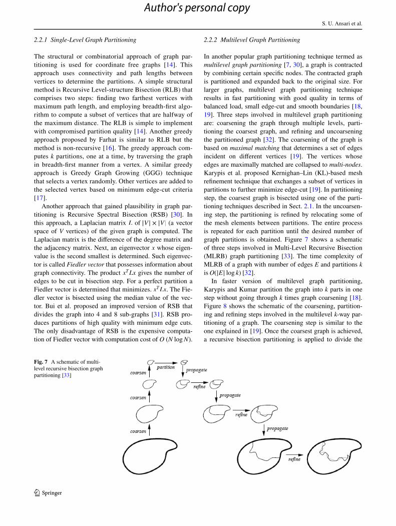
In another popular graph partitioning technique termed as multilevel graph partitioning [7, 30], a graph is contracted by combining certain specific nodes. The contracted graph is partitioned and expanded back to the original size. For larger graphs, multilevel graph partitioning technique results in fast partitioning with good quality in terms of balanced load, small edge-cut and smooth boundaries [18, 19]. Three steps involved in multilevel graph partitioning are: coarsening the graph through multiple levels, parti-tioning the coarsest graph, and refining and uncoarsening the partitioned graph [32]. The coarsening of the graph is based on maximal matching that determines a set of edges incident on different vertices [19]. The vertices whose edges are maximally matched are collapsed to multi-nodes. Karypis et al. proposed Kernighan–Lin (KL)-based mesh refinement technique that exchanges a subset of vertices in partitions to further minimize edge-cut [19]. In partitioning step, the coarsest graph is bisected using one of the parti-tioning techniques described in Sect. 2.1. In the uncoarsen-ing step, the partitioning is refined by relocating some of the mesh elements between partitions. The entire process is repeated for each partition until the desired number of graph partitions is obtained. Figure 7 shows a schematic of three steps involved in Multi-Level Recursive Bisection (MLRB) graph partitioning [33]. The time complexity of MLRB of a graph with number of edges E and partitions k is O(|E| log k) [32].

In faster version of multilevel graph partitioning, Karypis and Kumar partition the graph into k parts in one step without going through k times graph coarsening [18]. Figure 8 shows the schematic of the coarsening, partition-ing and refining steps involved in the multilevel k-way par-titioning of a graph. The coarsening step is similar to the one explained in [19]. Once the coarsest graph is achieved, a recursive bisection partitioning is applied to divide the

Fig. 7 A schematic of multi-level recursive bisection graph partitioning [33]



1 3

graph into k parts. In the refinement step a modified ver-sion of KL techniques are implemented. In KL technique a gain value for all the boundary vertices is computed by taking the difference between external degree and inter-nal degree of the graph. External degree is the sum of all weighted edges between the moving vertex in a partition and the vertices in other partitions. Similarly, the internal degree is the sum of all weighted edges between a moving vertex in a partition and the vertices inside the boundary of the same partition. The vertices with positive gain and the vertices that do not violate the balancing of the parti-tions are selected for migration. The scanning of the ver-tices is carried out using greedy KL refinement and global KL refinement [19]. In greedy KL refinement, the bound-ary vertices are traversed randomly and move a vertex with positive gain. However, the method of refinement lacks hill climbing strategy to avoid local minima, and thus the refinement algorithm settles with a suboptimal solution. The process of global KL refinement offers hill climbing strategy by storing vertices in a priority queue according to their gain and move the vertex with highest gain. If the bal-ancing conditions are not met, the vertex with second high-est gain is selected for movement. The time complexity of multi-level k-way partitioning (MLkP) is reduced to O(|E|) by a factor of log k when compared to MLRB.

Karypis et al. presented parallel implementation of coarsening, partitioning and refining of multilevel k-way partitioning [10, 13, 23]. Karypis et al. have used graph coloring to produce disjoint sets of vertices to simultane-ously coarsen and uncoarsen the graph on multiple proces-sors [10, 23]. The coloring of graph, that is a computation-ally intensive process, is implemented using Luby’s parallel algorithm [34]. In the coarsening step, vertices with the

same color are matched iteratively. A variable is defined for each vertex that stores the index number of the matched vertex. Colored graph resolve the issue of selecting various vertices for matching. Moreover, in partitioning phase, the parts of the coarsest graph are broadcasted using all-to-all operation (i.e., sends data from all-to-all processors). Fur-thermore, each processor partitions the graph using nested dissection [35] and greedy partitioning refinement. The nested dissection is a divide-and-conquer heuristic for the solution of sparse symmetric systems of linear equations using graph partitioning. The nested dissection gives worse partitioning when compared with serial recursive bisec-tion, however, it takes less time. The partition quality can be improved by mesh refinement in the uncoarsening phase [10, 23]. In uncoarsening phase, the vertices in the coarser graph are projected to the finer graph followed by partition-ing refinement. The parallel refinement approach is similar to the greedy refinement except the step of moving a group of vertices simultaneously [19]. The vertices of the same color make an independent set that are considered for the movement. Moreover, a subset of these vertices with posi-tive gain is moved to other partitions. The sum of individ-ual gain of each vertex is the overall gain of the group of vertices moved. However, the movement of group of ver-tices involves extensive inter-processor communication. To minimize the inter-processor communication, only the par-tition number associated with a vertex is changed without physically moving the vertex. The refinement process con-tinues in a loop for all colors in the graph [10, 13, 23]. The load balance constraint is also maintained by monitoring the continuously updated partition weight for every move-ment of the vertices [10, 13, 23].

Karypis and Kumar extended multilevel partitioning from single objective/single constraint to multi-constraint graph partitioning [20]. Single objective/single constraint graph partitioning can be defined as the partitioning of a graph where the objective is to minimize edge cut and the constraint is to balance the number of vertices [10, 23]. Multi-constraint graph partitioning has more than one con-straint. Karypis et al. have proposed two approaches for multi-constraint multilevel graph partitioning: multilevel recursive bisection for partitioning into two sub-graphs, and multilevel k-way partitioning for k sub-graphs [20]. In coarsening step, two approaches can be taken to collapse vertices into multi-nodes: heavy edge heuristic, and bal-anced edge heuristic. In heavy edge heuristic, the uniform-ity of weight vector is determined by computing the differ-ence between maximum and minimum weights of edges. In balanced edge approach, the difference is taken with respect to the average weight of the vector [19]. In parti-tioning step, a graph growing bisection technique is used. First, a vertex is randomly selected and added into bucket A while the remaining vertices are added into bucket B. All

Fig. 8 Multilevel k-way partition [11]


S. U. Ansari et al.

1 3

vertices in bucket B are moved to m (size of the weight vec-tor) priority queues based on the maximum weight in the weight vector. Finally, depending on the relative order of the weights of graph B, a vertex is moved from the top of a specific priority queue. The movement of vertices contin-ues until the weight of the graph A is greater than or equal to the half of weight of the original graph. The refinement step is implemented differently in recursive bisection and k-way partitioning. In recursive bisection, two priority queues are maintained, one for each bucket for storing gains of moving the vertices. Depending on the relative weights of two buckets, a vertex is selected from a queue in a partition and moved to other partition. Whereas, in k-way partition-ing, a set V ′ is built that contains the boundary vertices in a partition. Another set V ′′ of all vertices in the neighborhood is formed which satisfies the minimum edge-cut criteria. A set V ′′′ is extracted from V ′′ that fulfills the load balancing constraint. From V ′′′ a vertex is moved to the partition that gives the minimum edge-cut.

Schloegel et al. proposed a parallel algorithm for static multi-constraint multilevel graph partitioning [11]. The multi-constraint parallelization is an extension of the paral-lelization of single constraint graph partitioning presented by Karypis et al. [7]. The only difference is the implemen-tation of the refinement phase during uncoarsening the graph. The refinement phase is parallelized in two phases: a group of vertices with the same color is moved to other partitions with an update of a temporary data structure, and the balance constraints are validated after migration of ver-tices. If the balance constraints are not violated, the vertex movement is executed, otherwise, a portion of the moved vertices are recalled [20]. The recall may result in load imbalance. However, since the number of recalls is small, it is unlikely to have load imbalance after partitioning phase. The static partitioning can also be used effectively for dynamic multi-constraint multilevel graph partition-ing in conjunction with scratch-remap or locally matched scratch-remap. In dynamic load balancing, an additional constraint about minimization of data redistribution has to be satisfied. Initially, graph-based partitioning is imple-mented using sequential algorithm in the Metis library [18, 19]. The partitioning algorithm is parallelized using MPI library on distributed systems [10, 23]. LaSalle et al. extended graph partitioning to multithreaded algorithm for shared memory systems [6]. The multithreaded algorithms use multiple threads for independent computation but share the same data resources [36].

The so-called multilevel ant-colony algorithm, which is a relatively new metaheuristic search technique for solving optimization problems, was applied and studied in [37], and the possible parallelization of this algorithm is dis-cussed in [38]. The multilevel ant-colony algorithm per-formed well and is better than the classical k-METIS and

Chaco algorithms; it is comparable with the combined evo-lutionary/multilevel scheme used in the JOSTLE evolution-ary algorithm.

2.3 Solving System of Algebraic Equations

In an FEM system, a set of algebraic equations can be solved for unknown quantities using inverse of the stiff-ness matrix. However, taking inverse of a large and sparse stiffness matrix is a computationally expensive. Therefore, fast numerical techniques are used to determine the inverse matrix and solve for the unknown quantities. In the next two sections, some well-known linear and nonlinear equa-tion solving techniques are briefly discussed.

2.3.1 Linear System of Equations

Linear equation solving techniques can be classified as direct method and iterative method. The direct methods directly compute inverse of the stiffness matrix. These methods, however, become very expensive for large and sparse matrices. On the other hand, the iterative methods evaluate an approximate solution by updating the value of unknowns iteratively.

Direct approach

(i) Most commonly used direct method is called the Gaussian elimination method [39]. In Gaussian elim-ination method, the matrix is decomposed into upper and lower triangles using famous LU factorization [39].

(ii) The matrix decomposition can be made more effi-cient for some special matrices, such as, banded matrices or matrices that yield to Cholesky decompo-sition. The upper triangle is solved by backward sub-stitution of the computed coefficients. The drawback of Cholesky method is the propagation of round off errors originated from floating point operations [39].

(iii) The Gauss–Jordan elimination is a simple modifica-tion of the Gauss-elimination method that converts the coefficient matrix into reduced row echelon form [39]. The Gauss–Jordan method produces more accu-rate results in solving a system of linear equations and computing the inverse of the matrix simultane-ously.

Iterative approach

(i) One of the popular iterative methods is Jacobi method. The Jacobi method starts with an initial guess



1 3

to the solution and is solved iteratively until the solu-tion of desired precision is reached [40].

(ii) A more efficient iterative scheme is referred to as Gauss–Seidel iteration method [40]. In this method, the coefficient matrix is decomposed into lower and upper triangles before a variable is approximated. The decomposition matrix allows the Gauss–Seidel method to converge faster than the Gauss elimination method. However, the method is less stable and may oscillate indefinitely around the correct solution if the coefficient matrix is not strictly diagonally dominant [40]. Therefore, there is a trade-off between speed of convergence and the stability of the method [40].

(iii) Richardson method is another example of iterative method [1, 3]. In this method, � is a constant multi-plier and can be written as:

where I is an identity matrix. (5) leads to computation of parameter u in iterations as:

(iv) An iterative algorithm termed as conjugate gradient method is used for linear system of equations com-prising symmetric positive-definite matrix. The con-jugate gradient method is mostly employed for large sparse matrices that frequently result in the numerical (approximate) solution of BVPs [40, 41]. Suppose bn are n mutually conjugate vectors with respect to Ke forming a basis of ℝn in n dimensional real space, the solution to (16) can be expressed as:

If Ke in (16) is symmetric and positive definite then the coefficients �i can be computed as follows:

The quantity ⟨., .⟩ defines the inner product between two arguments. The first basis vector b0 is the negative of the gradient of f at an initial solution u0:

The second basis vector will be conjugate to the above gradient vector. Similarly, each new basis that is con-jugate to all the previously gradient vectors is com-puted iteratively.

(3)�Keui = �f e,

(4)ui +(�Ke − I

)ui = �f e,

(5)ui =(I − �Ke

)ui + �f e.

(6)ui+1 =(I − �Ke

)ui + �f e.

(7)u∗ =

n∑

i=1

�ibi.

(8)�i =⟨bi, f⟩⟨bi, biK⟩

.

(9)b0 = f − Ku0.

(v) The conjugate gradient method gives exact solutions. However, the conjugate method is unstable and the algorithm may oscillate around the exact solution [42, 43]. To stabilize the solution, a precondition matrix M, that is symmetric positive-definite and fixed, is used to compute the gradient vector. Multiplication of K with M results in the smaller condition number �(MK). The preconditioning leads to a well-known method called preconditioned conjugate gradient (PCG) to solve BVPs [42–45]. Mathematically, using (9), the PCG can be defined as follows:

2.3.2 Nonlinear System of Equations

Many physical systems, such as simulation of car crash, fluid–structure interaction and underground fluid flow, are inherently nonlinear. The nonlinear FEM systems result in nonlinear system of equations that are solved numerically [7]. The system of equations involving nonlinear functions, such as trigonometric, hyperbolic, exponential or logarith-mic functions, is called a system of nonlinear equations. The nonlinear equations are generally solved using numeri-cal techniques to produce inexact solution. The prime objective of these methods is to converge to exact solution in a smaller number of iterations with predefined error tol-erance � as discussed below:

(i) The most popular method for solving nonlinear equa-tions is Newtorn–Raphson method. Suppose the non-linear equation is presented as:

The solution of the above equation can be defined as:

The Newton–Raphson method iteratively computes improved solution of Eq. (12). The method requires initialization with one input value. If i is the iteration number, the general formula for iterative procedure for computing solution is given as:

Finally xi+1 is tested for convergence if the following condition is satisfied:

Newton–Raphson method converges quickly in rela-tively fewer numbers of iterations [46]. However, to

(10)b0 = M−1(f − Ku0).

(11)f (x) = 0

(12)|||f(xR)||| < 𝜀

(13)xi+1 = xi −f (xi)

f�(xi)

.

(14)|||f(xi+1

)||| < 𝜀.


S. U. Ansari et al.

1 3

use Newton–Raphson method one needs to compute the derivative of the given function.

(ii) The secant method is similar to Newton–Raphson method except the derivative of the given equation is approximated as:

Using Eq. (16) the secant method can be written as:

Equation (16) shows that, in contrast to Newton–Raphson method the secant method requires two ini-tial values as input to compute the current value of the solution.

(iii) The Richardson method discussed above can also be used for the solution of nonlinear equations if � is treated as a variable. Equation (6) converges if norm of I − �K is less than one. For maximum and mini-mum eigenvalues of K, �n and �1 respectively, the value of � is computed as:

(iv) In multi-physics, BVPs such as a moving structure in a fluid, the governing equations are first trans-formed into constrained variation problem. The prob-lem is converted into series of unconstrained prob-lems using Lagrange multiplier technique [47]. For instance, in an optimization problem, an objective function f (x, y) is needed to be maximized subject to the constraint g(x, y) = c for some constant c. The Lagrangian formulation can be written as:

where parameter � is called Lagrange multiplier. A penalty term � is added to Lagrangian formulation to retain the size of the system to that of primal vari-ables as:

The resulting expression in Eq. (19) is commonly referred to as augmented Lagrangian formulation [48, 49]. The augmented Lagrangian formulation can

(15)f�(xi)≈

f(xi)− f (xi−1)

xi − xi−1

(16)xi+1 = xi −f(xi)

f(xi)− f

(xi−1

) ⋅ (xi − xi−1).

(17)� =2

�n + �1.

(18)min�(x, y, �) = f (x, y) + �.(g(x, y) − c)

(19)min�(x, y, �,�) = f (x, y) + �.(g(x, y) − c)

+ �.((g(x, y) − c)2

).

be extended to multiple constraints, where � and � for each constraint have to be evaluated. If the (19) involves BVPs, it can be mapped to a discrete mesh and solved numerically using FEM.

2.4 Discussion

Various mesh partitioning techniques and a number of equation solving techniques for a distributed FEM system are reviewed. The following discussion compares and high-lights some of the intrinsic features of mesh partitioning methods and equation solving techniques that are crucial for the performance of a distributed FEM system.

2.4.1 Static Versus Dynamic Mesh Partitioning

If the number of FEM tasks to be distributed is fixed or change in a predictable fashion, the distribution can be done statically. A static mesh partitioning is a single-objective and single-constraint problem. The objective of the parti-tioning is to minimize the edge-cut while constraining the load balance. Such mesh partitioning is carried out prior to computations of mesh elements. Therefore, the partitioning can be done offline using sophisticated techniques that pro-duce better partitioning quality [50]. If the processing and memory requirements for a mesh computation are not too high, the static mesh partitioning can even be performed on a single processor.

The dynamic task distribution is used for load balancing if FEM workload on participating processors varies during the execution time. For instance, in adaptive mesh parti-tioning, the number of elements on each processor is modi-fied in runtime. Such runtime changes result load imbal-ance and require redistribution of mesh elements among PEs. The redistribution of mesh elements induces commu-nication overhead. For an efficient parallel system, the com-munication overhead must be kept minimum. Therefore, for dynamic mesh partitioning, time efficient algorithms are crucial to avoid deterioration of overall performance [50]. It is noteworthy that in dynamic mesh partitioning, the data is already distributed. Accordingly, the best strategy is to figure out the candidate elements that need to be relocated rather than gathering the entire mesh for repartitioning from scratch.

2.4.2 Spatial Versus Non-spatial Mesh Partitioning

A spatial FEM mesh is represented by a spatial grid with each node separated by a fixed distance [14]. The nodes



1 3

of the grid are described using (2D or 3D) spatial coordi-nates. The knowledge of spatial coordinates aids in defin-ing global relationship between elements. In spatial mesh, the proximity of elements is determined by computing, for instance, Euclidean distance [14]. In most cases, spatial distances truly represent the relationship between mesh ele-ments. However, in some cases, the path lengths between elements vary wildly from the computed spatial distances. Due to such discrepancies, the resulting partitioning from spatial methods may have quality issues [14]. Spatial meshes can also be transformed into graphs for employing graph theoretic partitioning techniques.

Non-spatial meshes cannot be distributed directly to a multiprocessor system due to their irregular geometry. Such meshes are initially mapped to some suitable struc-tures, such as, graphs before partitioning. The meshes represented by graphs can be distributed using graph-the-oretic partitioning algorithms. For instance, graph walking algorithm is a local-based graph traversing approach that allows access to the neighboring nodes. In such cases, sev-eral greedy techniques, such as greedy graph growing or graph growing bisection, are available to determine optimal graph partitioning. However, a greedy approach lacks the global view of a graph and possesses a potential tendency to fall into local minima [14]. To appease such problems, hill climbing methods may be incorporated into greedy techniques.

2.4.3 Graph Versus Tree Data Structures

Graph data structures are frequently used to represent spa-tial and non-spatial FEM meshes [19]. The graph represen-tation gives meshes an opportunity to use well established graph-theoretic approaches for mesh partitioning. The par-titioning of spatial meshes using graphs exploits geometri-cal topology of the meshes for improving partition quality [14]. Non-spatial graphs rely on neighborhood connectivity of the nodes and use greedy approaches for mesh partition-ing [19]. Graphs can be used in static as well as in dynamic mesh partitioning [11].

Tree data structures are commonly employed by spatial meshes in dynamic mesh partitioning [7, 9, 22–27]. Two- and three-dimensional FEM meshes can be conveniently mapped into quadtree and octree respectively. In tree-based partitioning, the tree is transformed into a 1-D array using space-filling curves, such as, Morton or Peano–Hilbert curves [51]. The space-filling curves ensure that the nearby nodes are proximally near in the 1-D array. The resulting 1-D array is subsequently bisected to achieve balanced mesh partitions. In tree-based partitioning approaches, the

load imbalance can also be computed using breadth-first or depth-first traversal [9, 25, 27].

2.4.4 Single Level Versus Multilevel Partitioning

For smaller meshes with uniformly distributed elements, the single level partitioning works more efficiently. In FEM mesh partitioning, there is a tradeoff between quality and complexity of mesh partitioning algorithm. Some mesh partitioning algorithms are less complex, such as recursive bisection or inertial bisection, however, the quality of par-titioning is compromised. Alternatively, more complex par-titioning algorithms, such as, recursive spectral bisection or refinement-based partitioning, generally produce partitions of optimum quality [14].

For large and non-spatial meshes, the multilevel par-titioning algorithms have proved to be faster with better partitioning quality [18, 19]. In multilevel partitioning, the coarsening and the uncoarsening steps take much less time than the partitioning of a mesh. Therefore, the multi-level partitioning is more economical and better than sin-gle-level partitioning if the size of the mesh is large [19]. Additionally, the coarsest mesh in multilevel partitioning is smaller compared to that of original one. Consequently, small meshes can afford more sophisticated mesh parti-tioning algorithms to improve quality [19]. Moreover, the refinement step in uncoarsening phase also aids partition-ing quality.

2.4.5 Serial Versus Parallel Partitioning

The mesh partitioning can be implemented offline in serial fashion using a single processor especially if the mesh size does not change [50]. Such mesh partitioning provides flexibility to employ complex and expensive algorithms to produce high quality partitioning. The partitioned mesh is subsequently distributed to processors for distributed FEM computations. Many of the algorithms developed for mesh partitioning are serial in nature. The advantages of serial approaches include no parallel computing overheads, such as, mesh partitioning and inter-processor communications among partitions. Small FEM meshes containing few thou-sand of elements do not generally require large memory and computing resources. Even if there is a need to dis-tribute the mesh over multiple processors, the partitioning of the mesh can be accomplished on a standalone machine either for static or dynamic meshes. Complex techniques for single-level partitioning, such as refine-based greedy approaches, can be employed for small meshes to achieve high partitioning quality.


S. U. Ansari et al.

1 3

In parallel implementation of FEM, some researchers assert that the available computing resources should also be utilized for partitioning of meshes [10, 29, 23]. Karypis et al. and Schloegel et al. proposed parallel multilevel mesh partitioning techniques to parallelize coarsening, parti-tioning and uncoarsening of a mesh [10, 11, 23]. Also, in dynamic mesh partitioning, a mesh is already in distributed form on multiple processors. The dynamic mesh partition-ing could be very costly if the mesh is gathered on a single processor and repartitioned repeatedly. Additionally, the number of elements to be migrated is small [7]. Therefore, it is wise to implement parallel dynamic mesh partition-ing scheme so that the redistribution of elements can be expedited. The large meshes pose a challenge in FEM solu-tion due to memory and processing power constraints. The natural choice for solving large meshes is to distribute the computing tasks over multiple processors. To take advan-tage of a parallel system, the partitioning algorithm should utilize the available computational power efficiently. The parallel algorithm implemented by Karypis et al. used less number of processors as it progresses in graph coarsening step [10]. In contrast, the parallel algorithm that Hussain et al. proposed utilizes all available processors in partition-ing a mesh [7].

2.4.6 Single-objective Versus Multi-objective Partitioning

The static mesh partitioning can be formulated as single-objective, single-constraint optimization problem with

an objective to minimize the edge cut under the con-straint of balanced partitioning [11]. In such problems, the physical properties of the domain do not change with time or space. There are many real life problems, such as, contact mechanics or crash simulation that include multi-phase and (multi-physics) domains. The FEM solution of such problems requires adaptive meshes which can be formulated as multi-objective, multi-constraint optimization problems. However, solving multi-objective, multi-constraint problems is generally challenging. An optimal solution is usually difficult to find due to the larger solution space, the large number of local optima, and the presence of often conflicting solutions.

2.4.7 Local Versus Global Partitioning

In greedy graph partitioning approaches, a partition tech-nique uses local information at the neighboring nodes to partition a mesh. Such approaches devoid information about the global structure of the mesh. The greedy par-titioning approaches are fast but have a potential to fall into local optima. The global information of the complete graph can be obtained from eigenvalues and eigenvectors of Laplacian matrix of the graph. The partition based on global information tends to be more accurate, however, requires more computations. For large FEM meshes, global partitioning techniques may be employed to partition the coarsest graph in multilevel graph partitioning.

Table 1 Comparison of Hussain et al. and Metis reordering algorithms using OpenMP

Procs Execution time (Hussain et al.)

EL = 15,625 EL = 12,167 EL = 10,648 EL = 8000 EL = 1000

1 2.94 2.21 1.94 1.42 0.17 4 0.62 0.56 0.50 0.37 0.04 8 0.38 0.29 0.25 0.19 0.03 12 0.28 0.21 0.18 0.14 0.02 16 0.23 0.17 0.15 0.12 0.02

Procs Execution time (Metis)

EL = 15,625 EL = 12,167 EL = 10,648 EL = 8000 EL = 1000

1 15.60 12.00 10.47 7.88 0.98 4 4.26 3.33 2.84 2.31 0.30 8 2.43 1.92 1.54 1.24 0.19 12 1.72 1.46 1.14 0.90 0.16 16 1.45 1.04 1.03 0.76 0.15



1 3

2.4.8 Computation Versus Communication

The distributed FEM computing provides large computing and storage resources. The parallel system gives an edge to the computation of complex scientific and engineering problems. Moreover, the parallel system with distributed memory also facilitates storage for problems with huge amount of data [36]. The parallel computation of distrib-uted tasks may require exchange of information between processors. Any form of communications between proces-sors is regarded overhead, and must be kept minimum to expedite the overall parallel processing [19]. Therefore, the main objective of the mesh partitioning techniques should be to minimize the inter-processor communications for effi-ciency and performance of a distributed FEM system.

Table 1 shows comparison of the two mesh reorder-ing algorithms for different meshes using OpenMP [52]. Table 2 summarizes the time complexities of various mesh partitioning algorithms on serial and parallel architectures (see Sect. 2.4.9).

2.4.9 Summary of Mesh Partitioning Techniques

The discussion so far deduces that there is no universal mesh partitioning method that works effectively and effi-ciently for all types of FEM meshes. Moreover, the mesh partitioning is highly application dependent, and there exists a trade-off between quality of partitioning (as a result of complex techniques) and partitioning speed [19, 30, 50]. In Table 3, a summary of the advantages and disadvantages of the mesh partitioning techniques is presented.

2.4.10 Equation Solvers Selection

The equation solvers take significant portion of FEM com-putations due to enormous size of coefficient matrices.

Therefore, a judicious selection of a solution is recom-mended. Often, the selection of an equation solver is based on the size and physics (linear or nonlinear) of the prob-lem on hand [53]. Other selection criteria for the equation solvers are symmetry, sparseness and of the coefficient matrix. In addition, a solver should be robust, general in scope, efficient, automated, scalable and predictable [53]. Direct methods used in equation solvers are robust but are computationally expensive. In contrast, iterative methods gradually converge to the optimal result based on speci-fied tolerance. The convergence tolerance should be chosen greater than the condition number of the coefficient matrix. If diagonal values of the coefficient matrix are close to zero (as is the case for sparse and ill-conditioned matrices), the computations become unstable. To ensure stability and accuracy, an equation solver should use ingrained proper-ties, such as, condition number, symmetry and positive definiteness, of the coefficient matrix. The diagonally dom-inant sparse coefficient matrices also minimize communi-cations between processors. A matrix can be converted into a diagonally dominant matrix using a pivoting scheme [53].

2.4.11 Equation Solvers’ Properties

In FEM, for steady state problems, the BVPs are trans-formed into a large system of algebraic equations. For sta-ble systems, the coefficient matrix is symmetric and posi-tive definite. Such properties of the matrix must be taken into account while solving the equations numerically to improve accuracy, stability and speed. The unstable sta-ble systems results in ill-conditioned or singular matrices that can be solved using a suitable matrix decomposi-tion method. Therefore, the type of solver used in FEM may also affect the overall performance of the system. In Table 4, a summssary of properties of equation solvers is presented.

Table 2 Time complexities of mesh partitioning techniques

Mesh partitioning technique Time complexity

Recursive orthogonal bisection [4] t(N) = O(d N logN)

Fiedler vector creation in recursive spectral bisection [30]

O(N logN)

Serial multilevel recursive bisection [32] O(|E| log k)Parallel multilevel recursive bisection [10] t(N) = O

(|E|Plog k

)

Serial multilevel k-way partitioning [18] O(|E|)Parallel multilevel k-way Partitioning [10] t(N) = O

(N

P

)+ O(P logN)

Serial mesh reordering [7] t(N) = O(N logN)

Parallel mesh reordering [7] t(N) = O(

N

P

)+ O(P logP) + O

(P2

)+ O

(N

Plog

N

P

)


S. U. Ansari et al.

1 3

Table 3 Summary of mesh partitioning techniques

Mesh partitioning technique Advantages Disadvantages

Spatial mesh partitioning Exploits geometry to capture global placement of vertices using spatial coordinates [14]

Geometrical distance between vertices may not be true descriptor of vertices proximity [14]

Non-spatial mesh partitioning Uses neighborhood of vertices for local con-nectivity [14]

Employ greedy approach for partitioning [16]

Blind to global placement of vertices [14]Vulnerable to local optima [16]

Single-level mesh partitioning Simple to implementFast for small meshes [16]

Slow for large meshesPoor partitioning quality for large meshes [7]

Multilevel mesh partitioning Efficient partitioning for large meshes [7]The refinement phase improves quality of parti-

tioning [19]

Complex in implementation due to coarsening and uncoarsening phases [7]

Partitioning of the coarsest mesh compromises quality [7]

Partitioning using optimization methods Multilevel ant-colony optimization works better than k-metis [83]

Fundamental issue with optimization methods is falling into local minima

Graph-based mesh partitioning Complex irregular FEM meshes are mapped to graphs [28]

Employs well-developed graph theoretic approaches for traversing and searching [29]

Uses only vertices connectivity for partitioning [14]

Could be costly in dynamic mesh partitioning [24]

Tree-based mesh partitioning Tree data structure assist in partitioning meshes [7]

Commonly employed in dynamic mesh partition-ing and mesh reordering [7]

Mapping of a mesh to a tree is time consuming [7]

Serial mesh partitioning Small meshes can be partitioned sequentially on a single machine [30]

No parallel overheadsSimple in coding

Not suitable for large meshes [11]Wastes computational and storage resources

Parallel mesh partitioning Utilizes available processing power and memoryAppropriate for large graphs for fast partitioning

[11]Employs well-known parallel libraries for shared

and distributed memory architectures [36]

Parallel overheads due to distribution of tasks [11]Complex implementation [11]Load balancing in an evolving distributed mesh is

complicated [11]

Single-objective mesh partitioning Most mesh partitioning is single objective and single constraint [7]

Easy to find optimal solution [30]Takes advantage of well-established optimization

theory [20]

Not suitable for multi-objective and multi-con-straint problems [20]

Multi-objective mesh partitioning Complex problems can be mapped to multi-objective, multi-constraint problems [20]

Helps in finding an optimal solution in large and difficult solution space [20]

Implementation is complexHighly potential for falling into local optima due to

large and multi-facet solution set [20]

Simple mesh partitioning Easy to program and modifyEasy to debugLess time consumingVery suitable for dynamic mesh partitioning [16]

May compromise quality of partitioning [16]

Complex mesh partitioning Produces good partitioning results [17] Complicated and requires longer time for execution [17]

Hard to code and debug [14]Mesh reordering Improves performance for distributed irregular

meshes by increasing cache hit rate [7]Time complexity is comparable to multilevel

mesh partitioning [7]

May not give significant results for regular meshes [7]



1 3

References

1. Hussain M, Kavokin A, (2009) A 2D parallel algorithm using MPICH for calculation of ground water flux at evaporation from water table. In: proceedings of FIT’09, Abbottabad.

2. Hussain M, (2011) ALE moving mesh generation and high per-formance implementation using OpenMP and MPI libraries for FSI and Darcy flow problems, PhD Thesis, Faculty of Computer Science and Engineering, Ghulam Ishaq Khan Institute

3. Hussain M, Kavokin A (2012) A calculation of 3D model of ground water flux at evaporation from water table using parallel algorithm—MPICH. Int J Math Phys 3(2):128–132

4. Salmon JK (1991) Parallel Hierarchical N-Body Methods,” PhD Thesis, California Institute of Technology

5. Keyser JD, Roose D (1992) Grid partition by inertial recursive bisection. Department of Computer Science, K. U. Leuven, Leuven

6. LaSalle D, Karypis G (2013) Multi-threaded graph partition-ing. 27th IEEE international parallel and distributed processing symposium

7. Karypis G, Kumar V (1996) Parallel multilevel k-way parti-tioning scheme for irregular graphs. In: Proceedings of IEEE Supercomputing

Table 4 Properties of numerical equation solvers

Type of equations Approach Methods Properties

Linear Direct approach for dense matrices [39] Gaussian elimination—LU factoriza-tion Requires

2

3n3 flops in transforming matrix

into echelon formGaussian elimination—Cholesky

decomposition Requires n3

3 flops and exploits symmetric positive definite property of the stiff-ness matrix

Gauss–Jordan methodRequires

4

3n3 flops, twice as many as

Gaussian elimination due to transfor-mation of stiffness matrix into reduced echelon form

Direct approach for sparse matrices Gaussian elimination For sparse matrix the time complexity reduces to O

(n1.5

) for 2D and O

(n2) for

3D meshesIterative approach for large sparse

matricesJacobi method Time complexity is O

(n2), solution may

diverge if the stiffness matrix is not strictly diagonally dominant [40]

Gauss–Seidel method -ditto-Richardson method Guarantees to converge if the norm of

I − �K is less than 1 for a stiffness matrix Kan arbitrary constant � [40]

Conjugate gradient method Faster than gradient descent method, converges in n steps, may take more than n steps or fail due to round off errors [40]

Preconditioned conjugate gradient method

Preconditioning improves convergence speed and stability [7]

Nonlinear Iterative approach for large sparse matrices

Newton–Raphson method Requires to compute derivatives, con-verges very fast if

||||f��(x)

f�(x)

|||| is not too large for a variable x [46]

Secant method Faster and more stable than Newton method and does not require deriva-tives, requires two initial points [46]

Regula–Falsi method Unlike Newton and secant methods root bracketing is guaranteed here [46]

Lagrange multiplier method Constrained optimization that works if critical points (maxima or minima) exist [47]

Augmented Lagrange multiplier Enjoys well established unconstrained optimization methods, however, the penalty coefficient should not increase without bound, otherwise, the unconstrained problem will become ill-conditioned [49]


S. U. Ansari et al.

1 3

8. Gilbert JR, Miller GL, Teng SH,(1995) Geometric mesh parti-tioning: implementation and experiments. In: proceedings of the 9th international parallel processing symposium, IEEE Com-puter Society Press, 418–427

9. Flaherty JE, Loy RM, Shephard MS, Szymanski BK, Teresko JD, Ziantz LH (1997) Adaptive local refinement with octree load balancing for the parallel solution of three-dimensional conservation laws. J Parallel Distrib Comput 47(2):139–152

10. Karypis G, Kumar V (1998) A parallel algorithm for multi-level graph partitioning and sparse matrix ordering. J Parallel Distrib Comput 48:71–85

11. Schloegel K, Karypis G, Kumar V (2002) Parallel static and dynamic multi-constraint graph partitioning. Concurr Comput 14:219–240

12. Boman EG, Catalyurek UV, Chevalier C, Devine KD, Safro I, Wolf MM (2009) Advances in parallel partitioning, load bal-ancing and matrix ordering for scientific computing. J Phys 180:12008

13. Karypis G, Schloegel K (2013) PARMETIS: parallel graph par-titioning and sparse matrix ordering library, version 4.0. Univer-sity of Minnesota, Minneapolis

14. Hussain M, Abid M, Ahmad M, Hussain SF (2013) A parallel 2D stabilized finite element method for darcy flow on distributed systems. World Appl Sci J 27(9):1119–1125

15. George A, Liu JW (1981) Computer solution of large sparse pos-itive definite systems. Prentice-Hall, Upper Saddle River

16. Farhat C (1988) A simple and efficient automatic FEM domain decomposer. Comput Struct 28(5):579–602

17. Pothen A, Simon HD, Liou K (1990) Partitioning sparse matri-ces with eigenvectors of graphs. SIAM J Matrix Anal Appl 11(3):430–452

18. Karypis G, Kumar V (1998) Multilevel k-way partition-ing scheme for irregular graphs. J Parallel Distrib Comput 48:96–129

19. Karypis G, Kumar V (1999) A fast and high quality multilevel scheme for partitioning irregular graphs. SIAM J Sci Comput 20(1):359–392

20. G. Karypis, V. Kumar (1998) Multilevel algorithm for multi-constraint graph partitioning.In: proceedings of ACM/IEEE on Supercomputing, 1–13

21. Hussain M, Abid M, Ahmad M (2012) Stabilized mixed finite elements for Darcy’s law on distributed memory systems. In: proceedings of international symposium on frontiers of compu-tational sciences, Islamabad. pp. 39–47

22. Chamberlain BL (1998) Graph partitioning algorithms for dis-tributing workloads of parallel computations. Technical Report UW-CSE-98-10-03, University of Washington

23. Karypis G, Kumar V (1999) Parallel Multilevel k-way partition-ing scheme for irregular graphs. SIAM J Comput 41(2):278–300

24. Warren MS, Salmon JK (1993) A parallel hashed oct-tree N-body algorithm. In: proceedings of supercomputing’93, ACM New York, NY,pp. 12–21

25. Flaherty JE, Loy RM, Ozturan C, Shephard MS, Szymanski BK, Teresko JD, Ziantz LH (1998) “Parallel structures and dynamic load balancing for adaptive finite element computation”. Appl Numer Math 26(1): 241–263

26. TU T, O’Hallaron DR, Ghattas O, Scalable parallel octree mesh-ing for terascale applications. In: proceedings of ACM/IEEE SC05, 2005

27. Mitchell WF (2007) A refinement-tree based partitioning method for dynamic load balancing with adaptively refined grids. J Par-allel Distrib Comput 67(4):417–429

28. Pellegrini F (2011) Current challenges in parallel graph parti-tioning. C R Mecanique 339:90–95

29. Bichot E, Siarry P (2013) Graph partitioning. Wiley, Hoboken, pp. 81–114

30. Hendrickson B, Leland R (1995) An improved spectral graph partitioning algorithm for mapping parallel computations. SIAM J Sci Comput 16(2):452–469

31. Bui T, Jones C (1993) A heuristic for reducing fill in sparse matrix factorization. In: proceedings of the 6th SIAM conference on parallel processing for scientific computing, pp. 445–452

32. Barnard ST (1995) A fast multilevel implementation of recursive spectral bisection for partitioning unstructured problems 1995

33. Barnard ST, Simon HD (1994) A fast multilevel implementation of recursive spectral bisection for partitioning unstructured prob-lems. Concurr Pract Exp 6(2):101–117

34. Luby M (1986) A simple parallel algorithm for the maximal independent set problem. SIAM J Comput 15:1036–1053

35. George A (1973) Nested dissection of a regular finite element mesh. SIAM J Num Anal 10:345–363

36. Grama A, Gupta A, Karypis G, Kumar V, (2003) Introduction to parallel computing. 2nd edn Addison-Wesley, Boston

37. Korošec P, Šilc J, Robič B (2004) Solving the mesh-partition-ing problem with an ant-colony algorithm. Parallel Comput 30(5–6):785–801

38. K. Taškova, P. Korošec, J. Šilc (2008) A distributed multilevel ant colonies approach. Informatica. 32(3):307–317

39. Davis TA (2006) Direct methods for sparse linear systems SIAM, Philadelphia

40. Saad Y (2003) Iterative methods for sparse linear systems. SIAM, Philadelphia

41. Ansari SU, Hussain M, Rashid A, Mazhar S, Ahmad SM (2015) Stabilized mixed galerkin method for transient analysis of Darcy flow. ICMSAO’15, Istanbul pp. 27–29

42. Hussain M, Ahmad M, Abid M, Khokhar A (2009) Implementa-tion of 2D parallel ale mesh generation technique in fsi problems using openmp. In: proceedings of fit’09, Abbottabad

43. Hussain M, Abid M, Ahmad M, Khokhar A, Masud A (2011) A parallel implementation of ALE moving mesh technique for FSI Problems using OpenMP. Int J Parallel Progr 30:717–745

44. Muhammad A, Khan A, Nash D, Hussain M, Wajid HA (2015) Simulation of optimized bolt tightening strategies for gasketed flanged pipe joints. In: proceedings of 14th International Confer-ence on Pressure Vessel Technology, 23–26 September

45. Muhammad A, Khan A, Hussain M, Wajid HA (2015) Optimized bolt tightening procedure for different tighten-ing strategies—FEA study. Proc Inst Mech Eng Part E. doi:10.1177/0954408915589687

46. Woodfords C, Philips C, (2012) Numerical methods with worked examples: Matlab edition. 2nd ed, Springer, Dordrecht

47. Lagrange JL (1811) Mécanique Analytique sect. IV 2 vol. Paris 48. Masud A, Bhagvanwala M, Khurram RA (2005) An adaptive

mesh rezoning scheme for moving boundary flows and fluid-structure interaction. Comput Fluids 36:77–91

49. Glowinski R (2008) Numerical methods for nonlinear variational problems Springer, Berlin/Heidelberg

50. Hendrickson B, Devine K (2000) Dynamic load balancing in computational mechanics. Comput Methods Appl Mech Eng 184(2–4):485–500

51. Schamberger S, Wierum JM (2005) Partitioning finite element meshes using space-filling curves. Future Gener Comput Syst 21:759–766

52. Ansari SU, Hussain M, Rashid A, Mazhar S, Ahmad SM (2015) Parallel stabilized mixed galerkin method for three-dimensional Darcy flow using openMp. NSEC Islamabad, Dec 17

53. Kaliakin VN (2001) Introduction to approximate solution tech-niques. In Numerical modeling, and finite element methods CRC Press


http://dx.doi.org/10.1177/0954408915589687

author's personal copy - ciit lahoreciitwah.edu.pk habibullah jamal [email protected] 1...

Documents