australian rainfall & runoff - geoscience...
TRANSCRIPT
Australian Rainfall & Runoff
Revision Projects
PROJECT 13
RATIONAL METHOD DEVELOPMENTS
Urban Rational Method Review
STAGE 3 REPORTDraft for discussion
P13/S3/001
FEBRUARY 2014

Engineers Australia Engineering House 11 National Circuit Barton ACT 2600 Tel: (02) 6270 6528 Fax: (02) 6273 2358 Email:[email protected] Web: www.engineersaustralia.org.au
PROJECT 13 STAGE 3: URBAN RATIONAL METHOD REVIEW
FEBRUARY, 2014
Project
Project 13: Urban Rational Method Review
AR&R Report Number
P13/S3/001
Date
12 February 2014
ISBN
Contractors
Dr Allan Goyen Cardno (NSW/ACT) Pty Ltd
Contractor Reference Number
W4913-002
Authors
Dr Allan Goyen Dr Brett C Phillips, Sahani Pathiraja
Verified by

Project 13: Rational Method Developments
P13/S3/001: 17 December 2013 i
ACKNOWLEDGEMENTS
This project was made possible by funding from the Federal Government through the Department of
Climate Change and Energy Efficiency. This report and the associated project are the result of a
significant amount of in kind hours provided by Engineers Australia Members.
CARDNO (NSW/ACT) PTY LTD
Level 9, 203 Pacific Highway ST LEONARDS NSW 2065
Telephone: 02 9496 7700 Facsimile: 02 9439 5170
Email: [email protected] Web: www.cardno.com.au

Project 13: Rational Method Developments
P13/S3/001: 17 December 2013 ii
FOREWORD
AR&R Revision Process
Since its first publication in 1958, Australian Rainfall and Runoff (ARR) has remained one of the most
influential and widely used guidelines published by Engineers Australia (EA). The current edition,
published in 1987, retained the same level of national and international acclaim as its predecessors.
With nationwide applicability, balancing the varied climates of Australia, the information and the
approaches presented in Australian Rainfall and Runoff are essential for policy decisions and projects
involving:
infrastructure such as roads, rail, airports, bridges, dams, stormwater and sewer
systems;
town planning;
mining;
developing flood management plans for urban and rural communities;
flood warnings and flood emergency management;
operation of regulated river systems; and
prediction of extreme flood levels.
However, many of the practices recommended in the 1987 edition of AR&R now are becoming
outdated, and no longer represent the accepted views of professionals, both in terms of technique and
approach to water management. This fact, coupled with greater understanding of climate and climatic
influences makes the securing of current and complete rainfall and streamflow data and expansion of
focus from flood events to the full spectrum of flows and rainfall events, crucial to maintaining an
adequate knowledge of the processes that govern Australian rainfall and streamflow in the broadest
sense, allowing better management, policy and planning decisions to be made.
One of the major responsibilities of the National Committee on Water Engineering of Engineers
Australia is the periodic revision of ARR. A recent and significant development has been that the
revision of ARR has been identified as a priority in the Council of Australian Governments endorsed
National Adaptation Framework for Climate Change.
The update will be completed in three stages. Twenty one revision projects have been identified and
will be undertaken with the aim of filling knowledge gaps. Of these 21 projects, ten projects
commenced in Stage 1 and an additional 9 projects commenced in Stage 2. The remaining two
projects will commence in Stage 3. The outcomes of the projects will assist the ARR Editorial Team
with the compiling and writing of chapters in the revised ARR.
Steering and Technical Committees have been established to assist the ARR Editorial Team in
guiding the projects to achieve desired outcomes. Funding for Stages 1 and 2 of the ARR revision
projects has been provided by the Federal Department of Climate Change and Energy Efficiency.
Funding for Stages 2 and 3 of Project 1 (Development of Intensity-Frequency-Duration information
across Australia) has been provided by the Bureau of Meteorology.

Project 13: Rational Method Developments
P13/S3/001: 17 December 2013 iii
Project 13: Rational Method Developments
Estimation of the peak flow on a small to medium sized rural catchment is probably one of the most
common applications of flood estimation as well as having a significant economic impact. While the
terms “small” and “medium” are difficult to define, upper limits of 25 km2 and 500 km
2 can be used as
guides. The Rational Method, which can be traced back to the mid-eighteenth century, is probably the
most commonly used method for estimating the peak flow of a flood. Most urban drainage systems
and culverts for rural roads, particularly those for small subdivisions, are designed using the Rational
Method.
However, there are a number of problems associated with the use of the Rational Method. Most of
these problems are associated with the estimation of parameter values such as the time of
concentration and the runoff coefficient. As a result, the rational method may be easy to implement,
but it is difficult to ensure that the predictions adequately represents processes occurring in the
catchment.
Mark Babister Associate Professor James Ball
Chair Technical Committee for AR&R Editor
ARR Research Projects

Project 13: Rational Method Developments
P13/S3/001: 17 December 2013 iv
AR&R REVISION PROJECTS
The 21 AR&R revision projects are listed below:
AR&R Project
No. Project Title
1 Development of intensity-frequency-duration information across Australia
2 Spatial patterns of rainfall
3 Temporal pattern of rainfall
4 Continuous rainfall sequences at a point
5 Regional flood methods
6 Loss models for catchment simulation
7 Baseflow for catchment simulation
8 Use of continuous simulation for design flow determination
9 Urban drainage system hydraulics
10 Appropriate safety criteria for people
11 Blockage of hydraulic structures
12 Selection of an approach
13 Rational Method developments
14 Large to extreme floods in urban areas
15 Two-dimensional (2D) modelling in urban areas.
16 Storm patterns for use in design events
17 Channel loss models
18 Interaction of coastal processes and severe weather events
19 Selection of climate change boundary conditions
20 Risk assessment and design life
21 IT Delivery and Communication Strategies
AR&R PROJECTS TECHNICAL COMMITTEE:
Chair: Mark Babister, WMAwater
Members: Associate Professor James Ball, Editor AR&R, UTS
Professor George Kuczera, University of Newcastle
Professor Martin Lambert, Chair NCWE, University of Adelaide
Dr Rory Nathan, SKM
Dr Bill Weeks, Department of Transport and Main Roads, Qld
Associate Professor Ashish Sharma, UNSW
Dr Bryson Bates, CSIRO
Steve Finlay, Engineers Australia
Related Appointments:
ARR Project Engineer: Monique Retallick, WMAwater
Assisting TC on Technical Matters: Dr Michael Leonard, University of Adelaide

Project 13: Rational Method Developments
P13/S3/001: 17 December 2013 v
EXECUTIVE SUMMARY
The broad aim of Project 13 Stage 3 was to consider the merits of the continued usage of the Rational
Method for estimating design flow peaks in urban catchments across Australia.
THE URBAN RATIONAL METHOD IN AUSTRALIA
The three editions of ARR (IEAust, 1958, 1977 and 1987) have each described the use of the urban
Rational Formula method. The main differences between the three editions have been the need to
assess partial area effects and the recommended procedures to estimate runoff coefficients and
overland flow times of concentration.
The 1958 ARR provided recommendations for the use of the Rational Formula based primarily around
the procedure introduced by Lloyd-Davies in England. Shortly after 1960 the original 1958 ARR
received a minor updating that included an amendment to the Figure which plotted the runoff
coefficients against rainfall intensity.
As described in the 1958 ARR:
“It is generally accepted that the values for the “coefficient of runoff are too high, primarily
because they do not make adequate allowance for storage effects. Reduced values are now
recommended. It is stressed, however, that these amended values are somewhat arbitrary,
and based on intuitive judgement rather than adequately controlled experiments”.
The 1977 ARR retained the same time of concentration procedure and runoff coefficients as included
in the 1958 ARR except for the change to metric units.
The 1987edition of ARR recommended changes to both the estimation of both time of concentration
and runoff coefficient in urban drainage design.
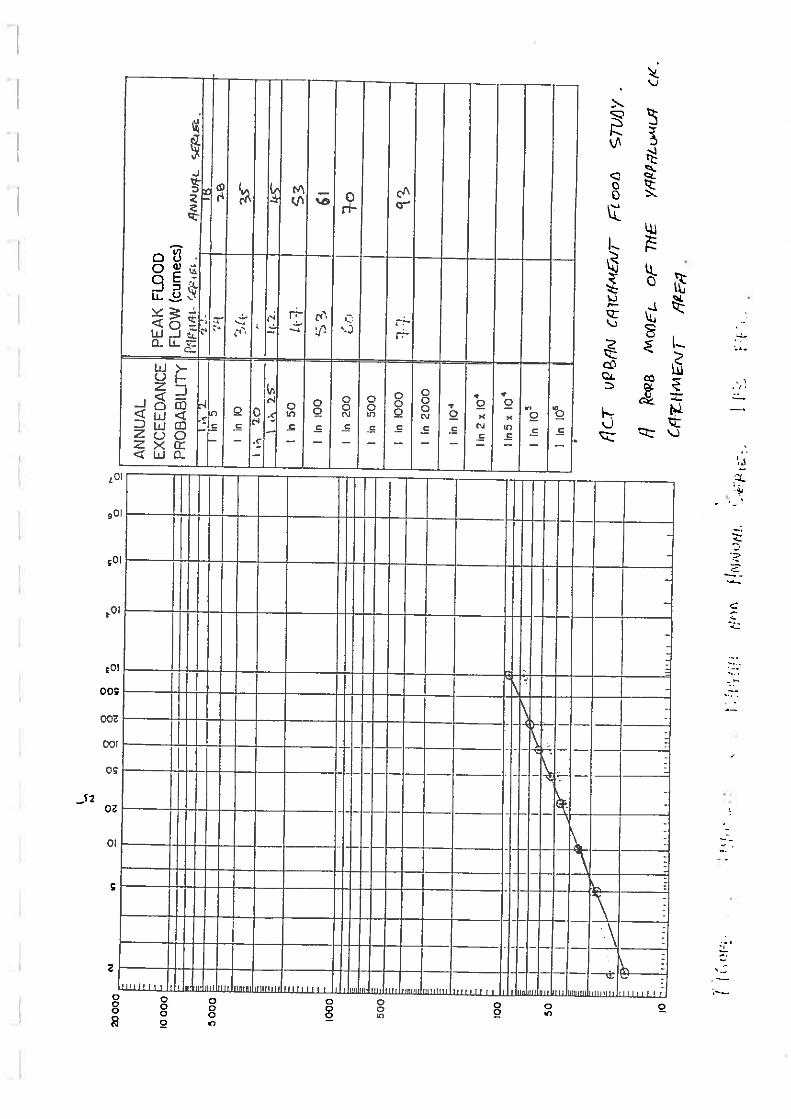
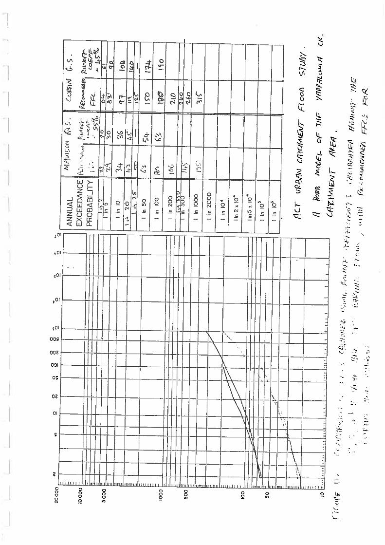
In late 1988 and early 1989 a study was undertaken in Canberra by the then Willing & Partners to
compare the methodologies for using the urban Rational Formula as recommended in both the 1977
and 1987 editions of Australian Rainfall and Runoff. Modelling was undertaken of both the Giralang
(64 ha urban in a 94 ha catchment) and Mawson (382 - 400 ha depending on storm severity) gauged
urban catchments and compared with flood frequency curves derived from gauged data. Both
gauged catchments had in excess of twelve years of runoff records in 1988.
In Giralang the 1977 recommendations were found to give a good fit to the gauged flood frequency
curve while the neither the runoff coefficient nor times of concentration for overland flow procedures
calculated using the 1987 procedures individually or in concert provided acceptable results. Analysis
of the Mawson catchment confirmed the findings from the Giralang catchment with the 1987
procedures giving peak design flows which were 40 - 60% lower than the flood frequency curve. In
effect, the 5 Yr ARI peak flood discharge predicted using the AR&R, 1987 procedures was in fact
equivalent to the gauged 1 Yr ARI peak flood discharge.

Project 13: Rational Method Developments
P13/S3/001: 17 December 2013 vi
In view of the absence of data to support the urban runoff coefficient estimation procedure proposed
in the 1987 ARR the comment of Munro (1956) may still apply:
"The literature abounds with tabulations of graphs of C for various conditions, but few
are observed from reliable evidence .... Apparently, Horner and Flynt (1936) are the
only ones to have carried out a really comprehensive set of measurements."
REVIEW OF GAUGED URBAN CATCHMENTS IN AUSTRALIA
The evolution of gauged urban catchments in Australia since the 1970s is overviewed in Section 3.
In 1977 a total of 69 urban catchments across Australia were being gauged in 1977 with a further 5
catchments being proposed for gauging (Black and Aitken (1977)). The breakdown of catchments
was:
ACT (Canberra) 7 NSW (Sydney) 3
QLD (Brisbane) 13 NT (Darwin) 3
VIC (Melbourne) 24 TAS (Hobart) 0
WA (Perth) 11 SA (Adelaide) 8
By 2009 only 24 urban gauged catchments were identified by Hicks et al. (2009) based on a number
of criteria:
Area less than 20 km2 (smaller areas preferable, in the order of 1 km
2);
Continuous records greater than 10 years in length;
Fairly urbanised (greater than 50%);
Acceptable gauge rating (max gauged flow: max recorded flow); and
Stationary upstream urbanisation.
The breakdown of gauged catchments is:
ACT (Canberra) 5 NSW (Sydney) 2
QLD (Brisbane) 3 NT (Darwin) 2
VIC (Melbourne) 3 TAS (Hobart) 2
WA (Perth) 2 SA (Adelaide) 5
Based on the review described herein it is recommended that:
(i) Engineers Australia consult with major stakeholders to formulate a strategy to ensure the
current collection of data is maintained and that data collection is expanded to encompass
representative urban catchments across Australia to ensure that sufficient good quality data is
available to allow the update of the Rational Formula method to reduce the potential error
levels in the peak flows estimated using the procedure and/or to improve the guidance on
rainfall-runoff model parameters for urban catchments;
(ii) Existing gauged urban catchments be reviewed to identify any features that may be distorting
gauging records (eg. basins) and that any review should include preliminary simulation
studies to quantify the effect of any features and the need or otherwise to develop a
procedure to correct the gauged data;

Project 13: Rational Method Developments
P13/S3/001: 17 December 2013 vii
(iii) Existing gauged catchments should be categorised based on regions, topography, geology
and/or drainage systems;
(iv) Identify possible urban catchments that could be gauged to provide data for any regions,
topography, geology and drainage systems not represented by existing gauged catchments;
(v) Undertake preliminary modelling of any new candidate gauged catchments;
(vi) Filter future potential gauged catchments to prioritize installations;
(vii) As a matter of priority seek to increase the density of rainfall gauges across existing gauged
catchments to further qualify areal effects within smaller urban catchments.
POSSIBLE USES OF CURRENT AVAILABLE GAUGED URBAN DATA
One of the objectives of this Discussion Paper was to identify potential uses of the gauged urban
streamflow data that is currently available. It was concluded that the current available gauged urban
streamflow data could be used to undertake Part I, Part II, Part III or Part IV studies as follows.
Part I Study
The Part I study approach is to calibrate relations for the estimation of time of concentration and
runoff coefficients for the urban Rational Method against flood quantiles derived from flood frequency
analysis (FFA) of flows recorded in one or more gauged urban catchments.
A Part I study was undertaken in the ACT in 1989 (refer Appendix E).
A key conclusion of the Part I study was that the runoff coefficient and time of concentration
relationships are paired ie. they both need to be derived concurrently using gauged data rather than
derived relationships independently.
The preliminary application of the Part I study approach to gauged urban catchments in Canberra,
Sydney, Melbourne and Darwin is described in Appendix C.
Part II Study
The Part II study approach is to calibrate parameter values for hydrological models by matching
predicted peak flows against flood quantiles derived from flood frequency analysis (FFA) of gauged
flows recorded in one or more gauged urban catchment.
A Part II study was undertaken in the ACT in 1993 (refer Appendix F).
In the case of the 1993 Part II study in the ACT it was found that in order to match the flow quantiles
obtained from FFA that the initial pervious rainfall loss needed to increase with increasing ARI ie. the
2 yr ARI peak flow was best fitted by a 5.0 mm initial pervious area rainfall loss while the 100 yr ARI
peak flow was best fitted by a 15.0 mm initial pervious area rainfall loss. This was counter-intuitive
and this issue was overcome by adopting a infiltration/water balance procedure based on the
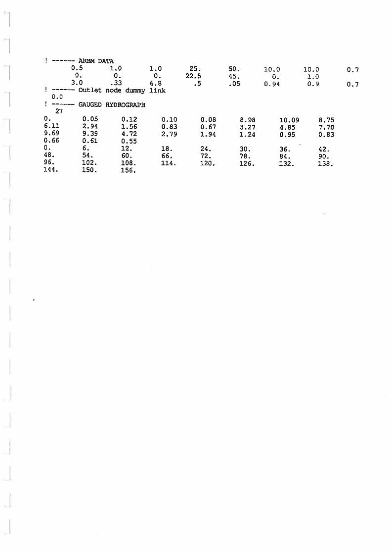
Australian Representative Basin Program (ARBM). A further potential problem with the Part II study in
the ACT was the recommended initial (high) values for moisture stores.

Project 13: Rational Method Developments
P13/S3/001: 17 December 2013 viii
These issues are explored in the analysis of the Giralang catchment (in Canberra) and Hewitt
catchment (in Sydney) in Appendix D.
Subsequent to the 1989 study Goyen (2000) incorporated an alternate sub-catchment analysis
procedure into the xprafts program. As presented in Appendix D, an excellent level of agreement was
achieved between gauged and predicted flows at the micro catchment and urban catchment scales in
Giralang and at the urban catchment scale in Hewitt by this model.
Part III Study
A possible approach to increase the number of test catchments would be to undertake rainfall and
flow gauging in new catchments for a period of 3-5 years only and to apply a Part III study approach
to create benchmark flood frequency curves for these new catchments as the basis for the testing of
runoff coefficient and time of concentration relations or identification of parameter values for
hydrological models ie. further Part I and/or Part II studies.
The Part III approach involves the calibration of a hydrological model (of the form assembled by
Goyen (2000) or a comparable model) against a range of storm events for which there is gauged
rainfall and runoff. A sufficient number of storm events would then be extracted from long term
pluviograph records and the calibrated model would be run to estimate peak flows. A FFA of the peak
flows could then be undertaken to estimate the flow quantiles.
This approach has been previously proposed by Aitken (1975) to utilize the available long term rainfall
pluviograph record nearest a catchment together with short term calibration records to simulate all the
major rainfall events in the rainfall record.
If multiple long term rainfall stations existed near or within the catchment the problems of rainfall
spatial variance could also be eliminated or at least minimized.
Part IV Study
The Part IV study approach is similar to the Part III study approach. However, instead of calibrating a
hydrological model (of the form assembled by Goyen (2000)) against a range of storm events for
which there is gauged rainfall and runoff, the hydrological model would be calibrated using full
continuous simulation for the period of gauging. This calibrated model would then be used to run the
long term pluviograph record(s) and predicted peak flows would then be extracted to allow a FFA to
be undertaken to estimate the flow quantiles.
Any continuous simulation would most likely rely on a scheme where the time step lengthens during
dry spells and reduces to a time step of say 1 minute during storm events.
APPLICATION OF THE URBAN RATIONAL METHOD
Should the Urban Rational Method continue to be included in ARR?
Since the publication of 1987 ARR a number of water authorities as well as Councils have also
published their own recommendations on how the Rational Method should be applied to urban
catchments in their jurisdiction. Typically these guidelines recommend procedures for estimating
runoff coefficient and time of concentration which differ from those recommended in the 1987 ARR. It
Project 13: Rational Method Developments
P13/S3/001: 17 December 2013 ix
is unclear if these guidelines are based on a comprehensive study of one or more gauged urban
catchments or whether values are somewhat arbitrary and based on intuitive judgement rather than
adequately controlled experiments (as concluded in the 1958 ARR).
Notwithstanding that the 1989 Part I study in the ACT concluded that the results from the study lent
further support to the continued use of the Rational Formula for drainage design in small to medium
sized urban catchments, this was on the basis that further studies be undertaken to further examine
possible modifications to the recommended 1987 ARR procedures to improve the estimation of
surface flow times of concentration and corresponding runoff coefficients. In particular, it
recommended that further studies should aim to determine appropriate surface roughness values for
use in the kinematic wave formulation for overland flow in Australia.
These further studies have not been undertaken in the 24 years since.
Notwithstanding the preliminary assessment of gauged urban catchments in Sydney, Melbourne and
Darwin disclosed that in general the 1977 ARR Rational Method gives peak flows which better match
the peak flows calculated by flood frequency analysis (FFA) than the peak flows estimated using 1987
ARR Rational Method (refer Appendix C) without carrying out Part I studies on a significant number of
additional gauged urban catchments it is the view of the authors that continued use of the Rational
Method for urban drainage analysis and design can no longer be justified.
Should the Urban Rational Method be used to Calibrate Hydrological Models?
With the advent of PCs in the 1980s and the improvements in computer speed and capabilities since
that time as well as the continued development of urban rainfall runoff catchment simulation models,
computer based modelling has almost totally supplanted the role of Rational Method calculations in
urban drainage design. Notwithstanding these advances some authorities still require urban
hydrological models to be “calibrated” to match peak flows estimated using the 1987 ARR urban
Rational Method.
It is the view of the authors that the urban Rational Method should not be used to calibrate urban
hydrological models unless it can be demonstrated that:
(i) A detailed Part I study has been undertaken on one or more gauged urban catchments in the
relevant city or town which has calibrated and validated relations for the calculation of runoff
coefficients and times of concentration; and
(ii) The urban catchment which is being modelled is subject to a similar hydrological regime and
has a level of imperviousness comparable to the gauged urban catchment(s) analysed in the
Part I study; and
(iii) WSUD measures are not present in the urban catchment which is being modelled.
CONSISTENCY WITH REGIONAL RURAL FLOOD METHOD
One of the objectives of this Discussion Paper was to investigate if it is practical to develop a method
to adjust the procedures recommended in Project 5 Regional Flood Methods to estimate peak flows in
small to medium sized urban catchments. .
An initial benchmark annual and partial series analysis of gauged flows has been undertaken for nine
urban catchments and one paired rural catchment as described in Appendix B. At the same time the

Project 13: Rational Method Developments
P13/S3/001: 17 December 2013 x
peak flows for each catchment under pre-development (rural) conditions for 2, 5, 10, 20, 50 and 100
yr ARIs were estimated for most of these catchments using the procedures recommended under
Project 5.
It was concluded from a comparison of flow quantiles for selected gauged urban catchments derived
from FFA and estimated peak flows for the selected catchments under rural conditions (estimated
using the Project 5 procedures) that:
The 2yr ARI peak flows for all urban catchments (derived from FFA) are higher than the
estimated 2 yr ARI peak flows under pre-development (rural) conditions (derived from
Project 5);
The ratio of urban to rural peak flows decreases as ARI increases;
In the case of the Canberra urban catchments the 100 yr ARI peak flow (derived from FFA)
are higher than the estimated 100 yr ARI peak flow under pre-development (rural) conditions
(derived from Project 5);
In the case of the Gungahlin paired rural catchment the Project 5 quantiles were consistently
and significantly higher than the corresponding FFA quantiles;
In the case of the Sydney, Melbourne, and Darwin urban catchments the 100 yr ARI peak flow
(derived from FFA) are lower than the estimated 100 yr ARI peak flow under pre-development
(rural) conditions (derived from Project 5).
It was further concluded that based on the scatter of the calculated ratios of urban to rural peak flows
and the overestimation of rural peak flows in comparison with urban peak flows derived from FFA in
major events in a number of catchments that it is not practical to develop a simple method to adjust
the peak flows from rural catchments to give reliable estimates of peak flows in urban catchments at
this time.

Project 13: Rational Method Developments
P9/S1/005: 12 February 2014
TABLE OF CONTENTS
............................................................................................................................................... Page
ACKNOWLEDGEMENTS (i)
FOREWORD (ii)
ARR PROJECTS (iii)
EXECUTIVE SUMMARY (iv)
TABLE OF CONTENTS
LIST OF TABLES
LIST OF FIGURES
1 INTRODUCTION ......................................................................................................... 1
1.1 AIM ..................................................................................................................................... 2
1.2 REPORT STRUCTURE ..................................................................................................... 3
2 URBAN RATIONAL METHOD IN AUSTRALIA .......................................................... 4
2.1 1958 EDITION .................................................................................................................... 4
2.2 1977 EDITION .................................................................................................................... 8
2.3 1987 ARR ........................................................................................................................... 8
2.4 DISCUSSION ................................................................................................................... 10
3 REVIEW OF GAUGED URBAN CATCHMENTS ....................................................... 12
3.1 GAUGED URBAN CATCHMENTS IN THE 1970s ........................................................... 12
3.2 GAUGED URBAN CATCHMENTS IN THE 1980s & 1990s ............................................ 14
3.3 GAUGED URBAN CATCHMENTS IN THE 2000s ........................................................... 14
3.4 DISCUSSION ................................................................................................................... 16
3.5 RECOMMENDATIONS .................................................................................................... 18
4 POSSIBLE USES OF CURRENT AVAILABLE GAUGED URBAN DATA ................ 19
4.1 PART I STUDIES.............................................................................................................. 19
4.2 PART II STUDIES............................................................................................................. 22
4.3 PART III STUDIES............................................................................................................ 23
4.4 PART IV STUDIES ........................................................................................................... 23
5 APPLICATION OF THE URBAN RATIONAL METHOD ........................................... 24
5.1 SHOULD THE URBAN RATIONAL METHOD CONTINUE TO BE INCLUDED IN ARR 24
5.2 SHOULD THE URBAN RATIONAL METHOD BE USED TO CALIBRATE
HYDROLOGICAL MODELS ............................................................................................. 25
6 CONSISTENCY WITH REGIONAL RURAL FLOOD METHOD ................................ 26
7 REFERENCES .......................................................................................................... 29

Project 13: Rational Method Developments
P9/S1/005: 12 February 2014
APPENDICES
APPENDIX A ARR PROJECT 5 REGIONAL FLOOD METHODS
APPENDIX B FLOOD FREQUENCY ANALYSIS IN SELECTED GAUGED URBAN
CATCHMENTS
APPENDIX C PRELIMINARY PART I STUDY – CANBERRA, SYDNEY, MELBOURNE, DARWIN
APPENDIX D PRELIMINARY PART II STUDY – CANBERRA & SYDNEY
APPENDIX E WILLING AND PARTNERS (1989) DRAINAGE DESIGN PRACTICE FOR LAND
DEVELOPMENT IN THE ACT. PART I: RATIONAL FORMULA PROCEDURES
APPENDIX F WILLING AND PARTNERS (1993) DRAINAGE DESIGN PRACTICE PART II

Project 13: Rational Method Developments
P9/S1/005: 12 February 2014
LIST OF TABLES
Table 1.1 Gauged Urban Catchment Descriptions (after 1987 ARR)
Table 1.2 Frequency Factors for Rational Method Runoff Coefficients
(after 1987 ARR)
Table 1.2 Gauged Urban Catchments in 1975 (after Aitken, 1975)
Table 1.2 Gauged Urban Catchments in Australia in 1977 (after Black and Aitken, 1977)
Table 1.3 Gauged Urban Catchments in Australia in 1989 (after Bufill, 1989)
Table 1.4 Gauged Urban Catchments in Australia in 2009 (after Hicks et al, 2009)
Table 1.5 2013 Study Catchment Details
Table 1.1 Estimated Urban and Rural Peak Flows in Selected Gauged Catchments
LIST OF FIGURES
Figure 1.1 Times for Surface Flow from Top of Catchment (after Figure 2-3, 1958 ARR)
Figure 1.2 Runoff Coefficients – Urban Catchments (after Figure 2-2, 1958 ARR)
Figure 1.3 Runoff Coefficients – Urban Catchments Amended (after Figure 2-2 (Amended), 1958
ARR)
Figure 1.4 10 year ARI Runoff Coefficients (after 1987 ARR)
Figure 1.2 Ratio of Urban to Rural Peak Flows against Urban Area
LIST OF ABBREVIATIONS
AEP Annual Exceedance Probability
ARI Average recurrence interval
ARR Australian Rainfall and Runoff
FFA Flood Frequency Analysis
QRT Quantile Regression Technique
RFFA Regional flood frequency analysis

Project 13: Rational Method Developments
P9/S1/005: 12 February 2014 1
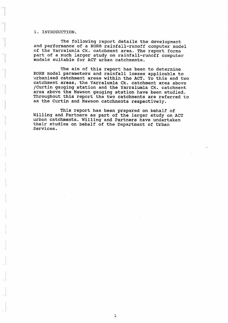
1 INTRODUCTION
Estimation of the peak flow on a small to medium sized rural catchment is probably one of the most
common applications of flood estimation as well as having a significant economic impact. While the
terms “small” and “medium” are difficult to define, upper limits of 25 km2 and 500 km
2 can be used as
guides. The Rational Method, which can be traced back to the mid-eighteenth century, is probably the
most commonly used method for estimating the peak flow of a flood. Most urban drainage systems
and culverts for rural roads, particularly those for small subdivisions, are designed using the Rational
Method.
The Rational Formula has been included in each of the Australian Rainfall and Runoff documents
since the release of the first edition in 1958. The method has been recommended for smaller urban
drainage design projects with an emphasis of providing a simple method that can be carried out
generally using hand calculations.
There are, however, a number of problems associated with the use of the Rational Method. Most of
these problems are associated with the estimation of parameter values such as the time of
concentration and the runoff coefficient. As a result, the Rational Method may be easy to implement,
but it is difficult to ensure that the predictions adequately represents processes occurring in the
catchment.
With the advent of PCs in the 1980s and the improvements in computer speed and capabilities since
that time as well as the continued development of urban rainfall runoff catchment simulation models,
computer based modelling has almost totally supplanted the role of hand calculations in urban
drainage design. Notwithstanding these advances some authorities still require urban hydrological
models to be “calibrated” to match peak flows estimated using the Rational Method.
In late 1988 and early 1989 a study was undertaken in Canberra by the then Willing & Partners to
compare the methodologies for using the urban Rational Formula as recommended in both the 1977
and 1987 editions of Australian Rainfall and Runoff.
The two documents differed significantly in their specific recommendations for estimating both the
subarea time of concentration for overland flow and the appropriate subcatchment runoff coefficient.
To test the acceptability of either the 1977 or 1987 recommendations, modelling was undertaken of
both the Giralang (64 ha urban in a 94 ha catchment) and Mawson (382 - 400 ha depending on storm
severity) gauged urban catchments and compared with flood frequency curves derived from gauged
data. Both gauged catchments had in excess of twelve years of runoff records in 1988.
In Giralang the 1977 recommendations were found to give a good fit to the gauged flood frequency
curve while the neither the runoff coefficient nor times of concentration for overland flow procedures
calculated using the 1987 procedures individually or in concert provided acceptable results. In the
Giralang analysis in particular, it was shown that it was essential to estimate peak flood flows from
partial areas. The peak flood flow at the catchment outlet was underestimated by 33% when only the
total area was considered.
Project 13: Rational Method Developments
P9/S1/005: 12 February 2014 2
To verify these findings, similar simulations were undertaken of the second gauged urban catchment
at Mawson. This catchment confirmed the findings from the Giralang catchment with the 1987
procedures giving peak design flows which were 40 - 60% lower than the flood frequency curve. In
effect, the 5 Yr ARI peak flood discharge predicted using the AR&R, 1987 procedures was in fact
equivalent to the gauged 1 Yr ARI peak flood discharge.
A number of lag times were also determined from recorded hydrographs from the Giralang and
Mawson gauging stations. These lag times lend further support to the acceptability of the AR&R,
1977 procedure for the estimation of surface flow times of concentration.
Notwithstanding that the 1989 review concluded that the results from the study lent further support to
the continued use of the Rational Formula for drainage design in small to medium sized urban
catchments this was on the basis that further studies be undertaken to further examine possible
modifications to the recommended AR&R, 1987 procedures to improve the estimation of surface flow
times of concentration and corresponding runoff coefficients.
In particular, further studies should aim to determine appropriate surface roughness values for use in
the kinematic wave formulation for overland flow in Australia.
These further studies have not been undertaken in the 24 years since.
In 1958 Professor Crawford Munro the lead author of the first edition of Australian Rainfall and Runoff
described in particular the runoff coefficients recommended in ARR as “intuition” based and nothing
has changed to date.
The proposition put forward by Tony Aitken in 1975 in AWRC Technical Paper 10 that Rational
Method parameters should be based on calibrated catchment simulation using long term rainfall
pluviograph data has now become practical, It is paradoxical that at a point in time when we can now
extract the maximum out of existing data collected over the last 40 years to recommend more factual
parameters for the Rational Method it is also the time to consider whether there is any merit in
continuing to clasp to the Rational Method for urban drainage system analysis or design.
1.1 AIM
The broad aim of Project 13 Stage 3 was to consider the merits of the continued usage of the Rational
Method for estimating design flow peaks in urban catchments across Australia.
This was considered in five steps as follows:
1. Assess the current availability of long term urban streamflow data to support the calibration
and verification of the urban Rational Method and the merit of continued collection of urban
streamflow data in the long term;
2. Identify appropriate uses of the gauged urban streamflow data that is currently available;
3. Identify possible limitations on the application of the urban Rational Method eg. catchment
size, event frequency, retarding basin analysis, etc and/or the need to include a factor of
safety when using the urban Rational Method;

Project 13: Rational Method Developments
P9/S1/005: 12 February 2014 3
4. Review the current practice of some authorities that require other hydrological methods to be
“calibrated” to the peak flows estimated using the using the urban Rational Method; and
5. Investigate if it is practical to develop a method adjust the procedures recommended in
Project 5 Regional Flood Methods to estimate peak flows in small to medium sized urban
catchments.
Related ARR Projects include:
ARR Project No. 13 Stage 1
ARR Project No. 5 Regional Flood Methods
1.2 REPORT STRUCTURE
This report is structured as follows:
Section 2 Urban Rational Method in Australia
Section 3 Review of Gauged Urban Catchments
Section 4 Possible Uses of Current Available Gauged Urban Data
Section 5 Application of The Urban Rational Method
Section 6 Consistency with Rural Regional Flood Method
Further information is also provided in the Appendices.

Project 13: Rational Method Developments
P9/S1/005: 12 February 2014 4
2 URBAN RATIONAL METHOD IN AUSTRALIA
The three editions of ARR (IEAust, 1958, 1977 and 1987) have each described the use of the urban
Rational Formula method. The main differences between the three editions have been the need to
assess partial area effects and the recommended procedures to estimate runoff coefficients and
overland flow times of concentration.
2.1 1958 EDITION
The first edition of ARR released in 1958 provided only two basic methods to estimate design flow
magnitudes within urban catchments in Australia. These were the Rational Method as prescribed by
Lloyd Davies for smaller urban drainage system design and the Unit Hydrograph procedure for larger
catchments for bridges and major drains. Both methods were considered to be deterministic models
of the rainfall-runoff process.
ARR, 1958 provided recommendations for the use of the Rational Formula based primarily around the
procedure introduced by Lloyd-Davies in England.
The Rational Formula for the peak discharge at the outlet of a drainage area was described as
(IEAust, 1958):
q = A C p (1)
where q = peak discharge (cusecs)
A = drainage area (acres)
C = a non-dimensional coefficient of runoff
p = temporal mean point-rainfall intensity (inches per hour) for a duration equal to the
time of concentration and for a specified storm recurrence interval.”
A nomograph and formula for the time of concentration was provided on Figure 2-3 in the 1958 ARR.
This nomograph is reproduced in Figure 2.1. Note the following attribution on the nomograph:
Data attributed to US Dept.of Agriculture. 1942,
Nomograph published in “Municipal Utilities”, Sept 1951
Formula and values of “n” added by J.A. Friend 19th Nov 1954.
For permeable areas the coefficient of runoff was plotted in Figure 2-2 in the 1958 ARR. This Figure
is reproduced in Figure 2.2.
Shortly after 1960 the original 1958 ARR received a minor updating that included an amendment to
Figure 2-2. The amended Figure 2-2 is reproduced in Figure 2.3. This figure changed from the
previous ASCE Hydrology Handbook figure to one based on a figure published by Ordon in 1954.
This amendment was described as follows: “Pending the collection of further data FIG 2-2 (amended)
is submitted as an interim improvement. This is the figure utilised by the metropolitan Water,
Sewerage and Drainage Board, Sydney N.S.W. and even this may give results somewhat on the high
side” ….

Project 13: Rational Method Developments
P9/S1/005: 12 February 2014 5
As described in the 1958 ARR:
“It is generally accepted that the values for the “coefficient of runoff are too high, primarily because
they do not make adequate allowance for storage effects. Reduced values are now recommended. It
is stressed, however, that these amended values are somewhat arbitrary, and based on intuitive
judgement rather than adequately controlled experiments”.
Figure 2.1 Times for Surface Flow from Top of Catchment (after Figure 2-3, 1958 ARR)

Project 13: Rational Method Developments
P9/S1/005: 12 February 2014 6
Figure 2.2 Runoff Coefficients – Urban Catchments (after Figure 2-2, 1958 ARR)

Project 13: Rational Method Developments
P9/S1/005: 12 February 2014 7
Figure 2.3 Runoff Coefficients – Urban Catchments Amended (after Figure 2-2 (Amended), 1958 ARR)

Project 13: Rational Method Developments
P9/S1/005: 12 February 2014 8
2.2 1977 EDITION
The 1977 edition of ARR retained the same time of concentration procedure and runoff coefficients as
included in the 1958 ARR except for the change to metric units.
The AR&R, 1958 nomograph also presented a formula for the calculation of the overland flow time
which was attributed to Friend, 1954. This equation is as follows (S.I. units):
to = 107 n L0.333
(2)
S0.2
where to = overland flow travel time (minutes)
L = flow path length (m)
n = Horton's roughness value for the surface
S = slope of surface (%)
2.3 1987 ARR
The 1987edition of ARR recommended changes to both the estimation of both time of concentration
and runoff coefficient in urban drainage design.
1987 ARR departed from the empirical relationship given in Equation 2. Instead, it recommended the
use of the "kinematic wave" equation for overland flow time previously described by Ragan & Duru
(1972). This equation is as follows:
to = 6.94 (L n*)0.6
I0.4
S0.3
(3)
where to = overland flow travel time (minutes)
L = flow path length (m)
n* = surface roughness
I = rainfall intensity (mm/h)
S = slope (m/m)
While the later equation for estimating overland flow times is based on a rigorous solution of the
shallow overland flow equations, the appropriate values particularly for the surface roughness, n*, are
not well defined. The reported roughness values for pervious surfaces range between 0.05 and 0.70.
Reported values for Horton's roughness values in Equation 3 are similar to Manning 'n' roughness
values and range between 0.015 for paved surfaces up to 0.06 for densely grassed surfaces.
The estimation of overland flow times can have a significant effect on the predicted peak flow due to
its influence on the value of rainfall intensity input into the Rational Formula.
The 1987 ARR varies from the 1958 and 1977 editions in its presentation of runoff coefficients for
design purposes. This edition presents a:
"composite relationship reflecting experience of drainage authorities and evidence from
the few gauged urban catchments with suitable lengths of record ..."

Project 13: Rational Method Developments
P9/S1/005: 12 February 2014 9
It is stated that:
"it should be used in preference to the runoff coefficient relationships given in previous
editions..."
The 10 Year ARI runoff coefficients recommended in the 1987 AR&R are presented in Figure 2.4.
Also shown for comparison are the data used to define the upper and lower bounds of the
interpolation zone. The location of the gauged catchments, their size and representative rainfall
intensity are given in Table 2.1.
Figure 2.4 10 year ARI Runoff Coefficients (after 1987 ARR)
Table 2.1 Gauged Urban Catchment Descriptions (after 1987 ARR)
Gauged Urban
Catchment No. Location
Catchment Area
(ha)
10I1
(mm/h)
1 Powells Creek, Strathfield, Sydney 231 48.9
2 Box Hill Main Drain, Box Hill, Melbourne 113 28.0
3 Vine Street Main Drain, Braybrook, Melbourne 70 29.0
4 Ashmore Ave Main Drain, Mordialloc, Melbourne 53 26.5
5 Gardenia Road Main Drain, Doncaster, Melbourne 80 28.1
6 Yarralumla Creek, Mawson, Canberra 382-400 32.2

Project 13: Rational Method Developments
P9/S1/005: 12 February 2014 10
The graphical relationship is further supplemented by the following numerical relationships:
C10 = 0.9 f + C110 (1 - f) (4)
and
C110 = 0.1 + 0.0133 (
10I1 -25) (5)
where C10 = 10 year ARI runoff coefficient
C110 = pervious area 10 Year ARI runoff coefficient
f = fraction impervious (0.0 to 1.0)
10
I1 = 10 year ARI, 1 hour rainfall intensity
For ARIs other than 10 years the C10 value is multiplied by a frequency factor from Table 2.2. Hence:
Cy = Fy C10 (6)
where Fy = Frequency factor.
Table 2.2 Frequency Factors for Rational Method Runoff Coefficients
(after 1987 ARR)
ARI (Years) Frequency Factor, Fy
1 0.80
2 0.85
5 0.95
10 1.00
20 1.05
50 1.15
100 1.20
In view of the absence of data to support the urban runoff coefficient estimation procedure proposed
in the 1987 ARR the comment of Munro (1956) may still apply:
"The literature abounds with tabulations of graphs of C for various conditions, but few
are observed from reliable evidence .... Apparently, Horner and Flynt (1936) are the
only ones to have carried out a really comprehensive set of measurements."
2.4 DISCUSSION
At the time of publication of the 1987 ARR the Rational Formula continued to attract wide spread use
both in Australia and overseas as indicated by Mein and Goyen (1988).
As indicated by Hicks et al (2009) the urban Rational Method presented in 1987 ARR remained in its
deterministic form notwithstanding a probabilistic version of the rural Rational Method was presented I
the 1987 ARR based on the fitting of regionally varying C values based on a large number of rural
gauged flow data records. This method was based on the research by Pilgrim and McDermott (1983)
who formulated a probabilistic version of the Rational Method for small rural catchments in Eastern
NSW.

Project 13: Rational Method Developments
P9/S1/005: 12 February 2014 11
It was considered in 1987 that there were insufficient gauged flow records to attempt to introduce a
regionally based probabilistic urban Rational Method.
During the consultation period held prior to the release of 1987 ARR a study was carried out in the
ACT at the request of the ACT Government to review the possible effects of differences between the
urban Rational Method procedures as recommended in 1977 ARR and 1987 ARR. This review is
described in a report titled “Drainage Design Practice for Land Development in the ACT. Part I:
Rational Formula Procedures”, Willing and Partners (1989) which is attached in Appendix E.
This report ultimately recommended a semi-probabilistic based procedure for urban drainage design
undertaken using the Rational Method in the ACT. The recommended procedure was based on the
outcomes of testing different combinations of the 1977 and 1987 procedures for estimating runoff
coefficient and time of concentration for estimating runoff coefficient to estimate flow peak quantiles in
two gauged urban catchments. The estimated flow quantiles were then compared with peak flows
determined using a flood frequency analysis. It was found that the combination of the procedures for
estimating runoff coefficient and time of concentration given in the 1977 ARR best fitted the flood
frequency curves from 2 yr ARI to 100 yr ARI.
The 1958 ARR provided a comprehensive procedure known as the "Tangent Check" to determine the
critical time for an area and the appropriate partial area to be applied in the Rational Formula
procedure. It was argued that a portion of the catchment area when multiplied by the higher rainfall
intensity resulting from a shorter time of concentration could provide a higher peak flow than the peak
flow contributed by the total area.
The 1977 ARR subjectively recommended against the use of partial area assessments including the
"Tangent Check" on the premise that the Rational Method was not accurate enough to warrant such a
check.
The 1987 ARR re-assessed the partial area question and recommended a single partial area check
by calculating a partial area based on the times of concentration of impervious zones directly
connected to the pipe system. Hence, 1987 ARR falls significantly short of the 1958 ARR
recommendations for the checking of partial areas.
This deficiency is particularly important since it has been previously reported (Willing & Partners,
1983) that peak flows in urban stormwater systems can be seriously underestimated by ignoring
partial area effects.
Since the publication of 1987 ARR a number of water authorities as well as Councils have also
published their own recommendations for how the Rational Formula should be applied to urban
catchments in their jurisdiction. Typically these guidelines recommend procedures for estimating
runoff coefficient and time of concentration which differ from those recommended in the 1987 ARR.

Project 13: Rational Method Developments
P9/S1/005: 12 February 2014 12
3 REVIEW OF GAUGED URBAN CATCHMENTS
The availability of good quality gauged data gauged in urban catchments is a pre-requisite to any
update of the Rational Formula method to reduce the potential error levels in the peak flows estimated
using the procedure and/or to provide guidance on rainfall-runoff model parameters.
Urban catchments with long term flow gauging of say over 20 years or more in Australia, as in most
western countries, are relatively rare. Even the number of urban catchments across Australia that
have been gauged for even shorter periods to facilitate the calibration of catchment models using
discrete storm events has also been limited.
The evolution of gauged urban catchments in Australia since the 1970s is overviewed as follows.
3.1 GAUGED URBAN CATCHMENTS IN THE 1970s
In 1975 only six urban or urbanising catchments were identified by Aitken in a study to investigate the
hydrology and design of urban stormwater drainage systems for the Australian Water Resources
Council Technical Paper No 10 (Aitkken, 1975)
These six catchments are reproduced in Table 3.1.
Table 3.1 Gauged Urban Catchments in 1975 (after Aitken, 1975)
Catchment Area (ha)
Urbanisation Fraction
Slope (%)
Vine Street, Main Drain, Victoria 76.7 1.00 0.22
Yarralumla Creek at Mawson, ACT 510 0.72 2.9
Yarralumla Creek at Curtin, ACT 2770 0.57 1.3
Elsternwick Main Drain, Victoria 3210 1.00 0.44
Bulimba Creek at Mansfield, Queensland 5440 0.25 0.31
Kedron Brook at Technical College, Queensland 5620 0.56 0.43
There was a very limited available data set however it still allowed the probable responses of the total
catchments to a number of individual gauged storm events to be investigated.
In a following AWRC study undertaken in 1977, Black and Aitken summarised the available gauged
urban catchments in Australia at the time. The table has been reproduced in Table 3.2. It discloses a
significant increase in the number of gauged urban catchments in comparison with the six catchments
identified by Aitken in 1975. In fact, a total of 69 urban catchments across Australia were being
gauged in 1977 with a further 5 catchments being proposed for gauging. The breakdown of candidate
catchments was:
ACT (Canberra) 7 NSW (Sydney) 3
QLD (Brisbane) 13 NT (Darwin) 3
VIC (Melbourne) 24 TAS (Hobart) 0
WA (Perth) 11 SA (Adelaide) 8

Project 13: Rational Method Developments
P9/S1/005: 12 February 2014 13
Black and Aitken, 1975 stated that on the basis of the listed gauged catchments the “the situation is
potentially a very good one”.
Table 3.2 Gauged Urban Catchments in Australia in 1977 (after Black and Aitken, 1977)

Project 13: Rational Method Developments
P9/S1/005: 12 February 2014 14
3.2 GAUGED URBAN CATCHMENTS IN THE 1980s & 1990s
Boyd et al (1994) included a table listing Australian as well as overseas gauged urban catchments.
Only nine gauged urban catchments in Australia were identified (refer to the first nine catchments
summarised in Table 3.3). A tenth catchment was analysed by Bufill, 1989 (refer Table 3.3).
It is unclear whether more catchments were available for the research undertaken by Bufill, 1989.
Table 3.3 Gauged Urban Catchments in Australia in 1989 (after Bufill, 1989)
Catchment Area (ha)
Imp Fraction.
No. of Events
Ratio of mean peak flows*
Maximum Event Difference Fraction
+
Qp (predicted) Qp (observed)
Negative Positive
Maroubra, NSW 57.26 0.52 39 0.97 0.62 2.05
Strathfield, NSW 234 0.50 78 0.94 0.30 1.63
Jamison Park, NSW 20.58 0.357 85 0.98 0.17 2.56
Fisher’s Ghost Creek, NSW 226 0.36 23 1.06 0.72 1.30
Giralang, ACT 96 0.25 14 0.77 0.29 1.05
Long Gully Ck, ACT 502 0.0478 14 - - -
Yarralumla Ck - Mawson, ACT 445 0.2584 11 0.84 0.56 1.34
Yarralumla Ck - Curtin, ACT 2690 0.1710 14 1.13 0.75 1.50
Vine Street, Victoria 70 0.314 11 1.21 0.83 1.5
Elster Ck, Victoria 3175 0.21 3 0.98 0.66 1.28
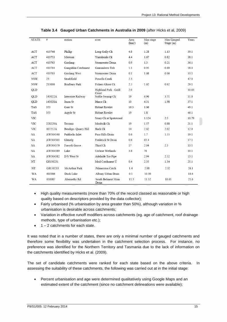
3.3 GAUGED URBAN CATCHMENTS IN THE 2000s
Hicks et al. (2009) identified 24 urban gauged catchments based on a number of criteria:
Area less than 20 km2 (smaller areas preferable, in the order of 1 km
2);
Continuous records greater than 10 years in length;
Fairly urbanised (greater than 50%);
Acceptable gauge rating (max gauged flow: max recorded flow); and
Stationary upstream urbanisation.
The table has been reproduced in Table 3.4. The breakdown of candidate catchments is:
ACT (Canberra) 5 NSW (Sydney) 2
QLD (Brisbane) 3 NT (Darwin) 2
VIC (Melbourne) 3 TAS (Hobart) 2
WA (Perth) 2 SA (Adelaide) 5
Most recently as part of an assessment of urban rainfall losses under ARR Project 6 Stage 2 – Losses
for Design Flood Estimation, the Hicks et al (2009) criteria were adopted for the identification of
candidate gauged urban catchments with some minor adjustments as follows:
Area less than 5km2 (500 ha), so that spatial variability in rainfall has less of an impact on the
analysis (due to the use of point rainfall data);
Record lengths of at least 10 years;
Project 13: Rational Method Developments
P9/S1/005: 12 February 2014 15
Table 3.4 Gauged Urban Catchments in Australia in 2009 (after Hicks et al, 2009)
High quality measurements (more than 70% of the record classed as reasonable or high
quality based on descriptors provided by the data collector);
Fairly urbanised (% urbanisation by area greater than 50%), although variation in %
urbanisation is desirable across catchments;
Variation in effective runoff modifiers across catchments (eg. age of catchment, roof drainage
methods, type of urbanisation etc.);
1 – 2 catchments for each state.
It was noted that in a number of states, there are only a minimal number of gauged catchments and
therefore some flexibility was undertaken in the catchment selection process. For instance, no
preference was identified for the Northern Territory and Tasmania due to the lack of information on
the catchments identified by Hicks et al. (2009).
The set of candidate catchments were ranked for each state based on the above criteria. In
assessing the suitability of these catchments, the following was carried out at in the initial stage:
Percent urbanisation and age were determined qualitatively using Google Maps and an
estimated extent of the catchment (since no catchment delineations were available);

Project 13: Rational Method Developments
P9/S1/005: 12 February 2014 16
Where available, data quality was analysed based on descriptors provided by the data
collector which consider the quality of measurement and correction methods.
Table 3.5 summarises the details of the selected urban catchments.
Table 3.5 2013 Study Catchment Details
State Catchment Name
Total
Area*
(TA) (ha)
Urban
Area^
(UA) (ha)
Total Impervious
Area
(TIA) (ha)
Urban
TIA
Fraction#
ACT Giralang 90.98 61.8 28.4 46%
NSW Powells Creek 231.9 223.4 151.7 68%
NT McArthur Park 143.7 120.2 53.7 45%
QLD Ithaca Creek 925.7 262.1 127.6 49%
SA Parra Hills Drain 55.1 48.5 26.9 55%
TAS Hobart City – Argyle Street 1,895.6 490.6 291.8 59%
VIC Kinkora Road 202.1 184.2 121.9 66%
WA Albany Drain near Duck Lake 8.2 8.2 2.9 35%
*Determined using the desktop GIS method
^The Urban Area is classified as the total developed area excluding large open space #The TIA fraction is defined as the percentage of impervious area in the urban area and was based on the
desktop GIS method.
3.4 DISCUSSION
It is obvious from the above overview of gauged urban catchments that the early predictions of Black
and Aitken (1977) that “the situation is potentially a very good one” has not been borne out over the
subsequent 35 years.
The obvious conclusion is that there still remains a scarcity of suitable gauged urban catchment with
sufficient data to update the Rational Formula method in order to reduce the potential error levels in
the peak flows estimated using the procedure. This is not to say that additional analysis using the
limited data already available could not lead to significant insights into the varying hydrologic
responses experienced in urban catchments across Australia.
As in 1975 there still remains an urgent need for the collection of long term rainfall and flow data in
gauged urban catchments to facilitate the updating of the Rational Method and/or other urban rainfall-
runoff estimation procedures. However before considering any additional gauging of urban
catchments in Australia it is important that the current catchments identified by Hicks et al, (2009) be
carefully reviewed to consider the utility of the data which has already been collected and/or identify
measures that need to be put in place to maximise the value of the data already collected and to be
collected in the future. This could include identifying the impact of any retarding basins or other
measures in a gauged urban catchment. A basin can modify the catchment runoff response by
infiltrating any overland flows into the grassed base of a basin in frequent events and by reducing
peak flows in major events eg. the basin in the McArthur Park catchment in Palmerston, NT.

Project 13: Rational Method Developments
P9/S1/005: 12 February 2014 17
In some cities such as Sydney for example, there may be also three or more distinct regions (eg.
coastal catchments on sand, inland catchments on heavier loam clays, catchments with steeper
slopes and/or ridgeline development only). Additionally drainage strategies can range from older
systems in older suburbs (eg. Powells Creek catchment) to newer suburbs (eg. Hewitt catchment)
only 30 km away, that includes a more contemporary, directly connected drainage scheme which in
some new subdivisions include significant WSUD measures.
To this end catchment simulation models should be established for each of the listed urban
catchments and an attempt be made to carry out a preliminary study on each similar to those
described in Appendix D. These studies would test the utility of the data already collected and
identify any issues with existing infrastructure that may distort the data or identify data that should be
also collected. This would allow either the addition of additional infrastructure to overcome any
existing problems or provide missing data or in some cases justify the cessation of the collection of
data at the current site. Additional catchments could then be considered with future gauging sites only
being selected after first passing a preliminary catchment analysis.
If the approach described in Sections 4.3 or 4.4 was adopted it may well be possible to minimize the
number of additional gauged catchments that would need to be established and monitored. Using
long term rainfall records rather than long term flow gauging records may allow short term (3-5 years)
snap shots of urban catchment which may be changing over time to be analysed to allow sufficient
calibration of a rainfall-runoff model that could then be used to estimate flow quantiles. It is
anticipated that there is a large amount of valuable event data available in many of the gauged
catchments identified above that could be extracted and used to facilitate the updating of the Rational
Method and/or other urban rainfall-runoff estimation procedures. This methodology is further
described in Section 4.3.
The first priority in any future gauging initiatives should be therefore to increase the number of
pluviographs located within existing gauged catchments to facilitate improved calibration of catchment
models.
It is important that any future gauging be recorded at time steps far shorter than 6 minute interval
which is currently accepted generally. This is extremely important for the simulation of urban
catchments less than say 300 ha in area.
Questions relating to future gauging that still need to be quantified include:
What is it worth to the taxpayer?
What is the return on investment?
Are there any future liabilities for Authorities and or Engineers Australia in recommending
design methods based on intuition rather than gauged data?
It would appear that past editions of ARR have not highlighted likely possible errors due to the
scarcity of data to quantify errors.
While the scarcity of data has continued the complexity of drainage systems continues to evolve. We
have moved from simple pipes and pits to widespread use of retarding basins, on-site detention
(OSD) and WSUD measures at lot, neighbourhood and regional scales. Additionally the average size
of lots has reduced substantially while the size of houses leading the imperviousness of urban
catchments to substantially increase over time.

Project 13: Rational Method Developments
P9/S1/005: 12 February 2014 18
Urban gauging in the past has been carried out by many different government and private
organizations at different times. This has often led to many gauging programs, which are
enthusiastically supported in the beginning, falling by the wayside before the maximum benefit could
be derived from the gauging program.
It may be possible Engineers Australia could co-ordinate or even project manage ongoing urban data
collection as a legacy of the current revision of ARR to ensure the next few decades provide far more
fruitful data then the last 30-40 years. This data could be then made available to universities and
hydrologists to support the development of improved urban flow estimation and design procedures.
The aim would be to significantly reduce the potential error bands when recommending suitable urban
drainage management solutions to meet both current and future demands in any urbanising
catchment in Australia. The challenge is how best to fund any data collection that will be sustainable
into the future.
3.5 RECOMMENDATIONS
Based on the review of gauged urban catchments in Australia since the 1970s it is recommended
that:
(viii) Engineers Australia consult with major stakeholders to formulate a strategy to ensure the
current collection of data is maintained and that data collection is expanded to encompass
representative urban catchments across Australia to ensure that sufficient good quality data is
available to allow the update of the Rational Formula method to reduce the potential error
levels in the peak flows estimated using the procedure and/or to improve the guidance on
rainfall-runoff model parameters for urban catchments;
(ix) Existing gauged urban catchments be reviewed to identify any features that may be distorting
gauging records (eg. basins) and that any review should include preliminary simulation
studies to quantify the effect of any features and the need or otherwise to develop a
procedure to correct the gauged data;
(x) Existing gauged catchments should be categorised based on regions, topography, geology
and/or drainage systems;
(xi) Identify possible urban catchments that could be gauged to provide data for any regions,
topography, geology and drainage systems not represented by existing gauged catchments;
(xii) Undertake preliminary modelling of any new candidate gauged catchments;
(xiii) Filter future potential gauged catchments to prioritize installations;
(xiv) As a matter of priority seek to increase the density of rainfall gauges across existing gauged
catchments to further qualify areal effects within smaller urban catchments.
Project 13: Rational Method Developments
P9/S1/005: 12 February 2014 19
4 POSSIBLE USES OF CURRENT AVAILABLE GAUGED URBAN DATA
One of the aims of this Discussion Paper was to identify potential uses of the gauged urban
streamflow data that is currently available. The current available gauged urban streamflow data could
be used to undertake Part I, Part II, Part III or Part IV studies of current gauged urban catchments as
discussed below.
4.1 PART I STUDIES
In 1989 a review the possible effects of differences between the urban Rational Method procedures
recommended in 1977 ARR and 1987 ARR was undertaken in the ACT (Willing & Partners, 1989).
This review is described in a report titled “Drainage Design Practice for Land Development in the
ACT. Part I: Rational Formula Procedures (Part I Study) which is attached in Appendix E.
This report ultimately recommended a semi-probabilistic based procedure for urban drainage design
undertaken using the urban Rational Method in the ACT. The recommended procedure was based on
the outcomes of testing different combinations of the 1977 and 1987 procedures for estimating runoff
coefficient and time of concentration for estimating runoff coefficient to estimate flow peak quantiles in
two gauged urban catchments. The estimated flow quantiles were then compared with peak flows
determined using a flood frequency analysis. It was found that the combination of the procedures for
estimating runoff coefficient and time of concentration given in the 1977 ARR best fitted the flood
frequency curves from 2 yr ARI to 100 yr ARI.
A key conclusion of the Part I study was that the runoff coefficient and time of concentration
relationships are paired ie. they both need to be derived concurrently using gauged data rather than
derived relationships independently.
Since 1989 additional data has been collected in the Giralang catchment which has allowed the
updating of the 1987 analysis as well as the preliminary testing of the sensitivity of the predicted peak
flows to characterising a catchment based on total impervious area (TIA) or effective impervious area
(EIA) as assessed in ARR Project 6 Stage 2 - Analysis of Effective Impervious Area & Pilot Study of
Losses in Urban Catchments.
The preliminary application of the Part I study approach to gauged urban catchments in Canberra,
Sydney, Melbourne and Darwin is described in Appendix C. The peak flows were estimated for
various representations of each urban catchment using a single node xprathgl model of each
catchment.
The conclusions from these preliminary analyses are as follows.
4.1.1 Canberra and Sydney
It was concluded from a comparison of the various Giralang catchment results that:
The 1977 ARR procedures give peak flows which match the peak flows adopted for the
composite series based on flood frequency analysis (FFA) except for flows based on EIA only;
For 10 yr ARI and above the 1987 ARR procedures give similar peak flows to the ARR Project
5 procedures for rural catchments;
Project 13: Rational Method Developments
P9/S1/005: 12 February 2014 20
The 1987 procedures give peak flows lower than the peak flows adopted for the composite
series based on flood frequency analysis with the estimated 100 yr ARI peak flow comparable
to the 10 yr ARI peak flow from the FFA;
It was concluded from a comparison of the various Hewitt catchment results that:
The 1977 ARR procedures give peak flows which are slightly lower than the peak flows adopted
for the composite series with the estimated 100 yr ARI peak flow being comparable to the 50 yr
ARI peak flow from the FFA.
The 1987 procedures give peak flows lower than the peak flows adopted for the composite
series with the estimated 100 yr ARI peak flow being comparable to the 10 yr ARI peak flow
from the FFA.
It was concluded from a comparison of the various Powells Creek catchment results that:
The 1977 ARR procedures give peak flows which are higher than the peak flows obtained from
an annual series analysis of gauged flows with the peak flows estimated for frequent runoff up
to 10 yr ARI being significantly higher;
One approach to improve agreement would be to test Curve No. 6 in comparison with the
adopted Curve No. 5;
The 1987 procedures give peak flows slightly higher than the peak flows adopted for the
annual series but in good agreement.
4.1.2 Melbourne
Based on the results presented in Table C.8 it is apparent all Rational Method peak flows are
significantly higher than corresponding flood frequency peak flow estimates except where agreement
is forced by adjusting the runoff coefficient or the time of concentration.
Based on the work of Pomeroy et al (2013) the Kinkora Road urban catchment shares many
characteristics with the Powells Creek urban catchment in Sydney. The peak flows in both
catchments appear to derive mostly from the EIA only. This may well encompass only the roads
themselves plus very limited amounts of in block hard surfaces.
This also highlights the potential problems of adopting a limited number of long term gauged urban
catchments as representative of all urban catchments. The Kinkora Road and Powells Creek
catchments are probably representative of many older suburbs which were first developed in the
1950s or 1960s. They are however not representative of newer catchments with high degrees of
directly connected impervious areas including the Hewitt catchment in Sydney and the Giralang
catchment in ACT.
4.1.3 Darwin
It should be noted that roof drainage guttering across the Moil catchment is very limited with the
majority of runoff simply falling into the allotment yard. It was concluded from a comparison of the
various results for the Moil catchment that:
The 1977 ARR procedures give peak flows which are slightly higher than the peak flows
adopted for the composite series (based on the adoption of Curve 6 for runoff coefficients);
Project 13: Rational Method Developments
P9/S1/005: 12 February 2014 21
The 1987 procedures give peak flows higher than the peak flows adopted for the composite
series for events greater than a 10 yr ARI event.
In the case of the McArthur Park catchment in Palmerston, it was found that most predicted peak
flows estimated using the 1977 ARR or 1987 ARR procedures gave peak flows considerably higher
than the peak flows estimated by FFA of the gauged flows from the McArthur Park catchment.
While one approach to improve agreement would be to test Curve No. 5 in comparison with the
adopted Curve No. 4 it was noted however that these FFA results are problematic due to the
presence of a large retarding basin located upstream of the gauging station which can modify
the runoff response from a significant proportion of the catchment by infiltrating any overland
flows into the grassed base of the basin in frequent events and by reducing peak flows in major
events.
4.1.4 Discussion
Since the publication of 1987 ARR a number of water authorities as well as Councils have also
published their own recommendations for how the Rational Formula should be applied to urban
catchments in their jurisdiction. Typically these guidelines recommend procedures for estimating
runoff coefficient and time of concentration which differ from those recommended in the 1987 ARR. It
is unclear if these guidelines are based on a comprehensive Part I study where the runoff coefficient
and time of concentration relationships were derived concurrently or are values which are somewhat
arbitrary and based on intuitive judgement rather than adequately controlled experiments (as
highlighted in the 1958 ARR).
It is apparent from a comparison of the discussion in Section 3 and Appendix A that in the past
considerably greater effort has gone into flow gauging in rural catchments compared to flow gauging
in urban catchments notwithstanding 70% of the population of Australia lives in Sydney, Melbourne,
Brisbane, Perth, Adelaide, Canberra, Hobart and Darwin.
Stage 2 of Project 5 has assembled a quality controlled national database consisting of 727 stations
located in rural catchments while Hicks et al (2009) identified 24 gauged urban catchments across
Australia ie. there are 30 rural flow gauging stations for every 1 urban gauging station in Australia.
The length of record at stations in urban catchments is also often restricted to 10 years or less.
As disclosed by Hicks et al (2009) the number of urban catchments (500 ha or less) with 20
years of records is only 11, with 30 years of record is 7, with 40 years of record is 4 and with 50
years record is 1 only.
Even if all the urban catchments listed in Table 3.4 were studied using the Part I Study approach this
would still only result in some 24 catchments to cover all of Australia. The results would also be
specific to each catchment’s hydrological regime, topography, geology and its stormwater drainage
management strategy.
A possible approach to increase the number of test catchments would be to undertake rainfall and
flow gauging in new catchments for a period of 3-5 years only and to apply a Part III or Part IV study
approach (refer Sections 4.3 and 4.4) to create benchmark flood frequency curves for these new
catchments as the basis for the testing of runoff coefficient and time of concentration relations within a
catchment ie. further Part I studies.
Project 13: Rational Method Developments
P9/S1/005: 12 February 2014 22
4.2 PART II STUDIES
In 1993 a study was undertaken in Canberra to provide practice guidelines when utilising hydrograph
based estimation procedures in urban drainage projects in the ACT (Willing & Partners, 1993). The
work followed on from the earlier Part I study. It is described in a report titled “Drainage Design
Practice Part II”, Willing and Partners (1993) which is attached in Appendix F.
The goal of the Part II study was to test several currently available rainfall/runoff computer programs
including RAFTS, RORB and IlSAX on Canberra's gauged urban catchments.
In particular, the objectives were to determine appropriate:
(i) design rainfall loss rate estimation parameters applicable to individual programs,
(ii) surface runoff routing parameters for pervious and impervious areas specific to each program
tested, and
(iii) design storm event modelling procedures specific to each program tested.
Since the 1993 study was completed an addition of 20+ years of rainfall and runoff data collected
including 3 years of data collected on micro catchments embedded within the Giralang urban
catchment. Data from the micro catchments was collected and reported in the PhD thesis submitted
by Goyen in 2000. The research reported by Goyen, 2000 further examined the processes within the
Giralang catchment as well as the Hewitt urban catchment located near Penrith in Sydney.
A potential problem with the Part II study in the ACT was the recommended initial (and high) values
for moisture stores. An embedded approach has been assessed to establish if it performs better than
fixed initial values in a vertical water balance loss model.
These issues are explored in the analysis of the Giralang catchment (in Canberra) and Hewitt
catchment (in Sydney) in Appendix D. These investigations applied a modified sub-catchment
hydrograph estimation module from xprafts as described by Goyen (2000).
The modifications to the xprafts analysis procedure included an alternate sub-catchment analysis
procedure that is indicated diagrammatically in Figure D.4. Runoff is estimated separately for the roof
and gutter, adjacent road surface and paving and pervious gardens and lawn areas. A virtual
allotment drainage network is constructed to represent lagging, bypass, capture and additional
storage routing and infiltration/ evapotranspiration within the various WSUD facilities. The outputs
from each structure as well as any bypass flows are combined to give the total runoff hydrograph from
a typical allotment.
The method allows the definition of a wide range of WSUD/LID facilities including allotment storage
devices, infiltration beds and rain water tanks. The procedures allows for variable structure sizes as
well as variable capture and bypass percentages. Additional parameters to define the percentage
breakdown in impervious surfaces between roofs, paving and road surfaces was also included.
The models as described by Goyen (2000) were adopted without any modification apart from the
addition of evaporation from impervious surfaces during the extended duration summer daytime
events.

Project 13: Rational Method Developments
P9/S1/005: 12 February 2014 23
An excellent level of agreement was achieved between gauged and predicted flows at the micro
catchment and urban catchment scale in Giralang and at the urban catchment scale in Hewitt.
As discussed in Appendix D, if the simulation of historical storms is able to match the observed
events as closely as achieved by Goyen (2000) in the Giralang catchment in the period 1993 – 1995
then the resulting flow quantiles obtained from FFA of the simulated peak flows should closely match
the flow quantiles derived from the gauged peak flows. This creates an opportunity to use a calibrated
hydrological model (of the form assembled by Goyen (2000)) to estimate peak flows from storm
events extracted from long term pluviograph records and to then undertake FFA of the synthetic peak
flows to estimate flow quantiles ie. a Part III or Part IV study approach.
This in turn could inform the determination of parameter values for other hydrological models (a Part II
study).
4.3 PART III STUDIES
A possible approach to increase the number of test catchments would be to undertake rainfall and
flow gauging in new catchments for a period of 3-5 years only and to apply a Part III study approach
to create benchmark flood frequency curves for these new catchments as the basis for the testing of
runoff coefficient and time of concentration relations within a catchment ie. further Part I and/or Part II
studies.
The Part III method involves the calibration of a hydrological model (of the form assembled by Goyen
(2000)) against a range of storm events for which there is gauged rainfall and runoff. A sufficient
number of storm events would then be extracted from long term pluviograph records and the
calibrated model would be run to estimate peak flows. A FFA of the peak flows could then be
undertaken to estimate the flow quantiles.
This approach has been previously proposed by Aitken (1975) to utilize the available long term rainfall
pluviograph record nearest a catchment together with short term calibration records to simulate all the
major rainfall events in the rainfall record.
If multiple long term rainfall stations existed near or within the catchment the problems of rainfall
spatial variance could also be eliminated or at least minimized.
4.4 PART IV STUDIES
The Part IV study approach is similar to the Part III study approach. However, instead of calibrating a
hydrological model (of the form assembled by Goyen (2000)) against a range of storm events for
which there is gauged rainfall and runoff the hydrological model would be calibrated using continuous
simulation for the period of gauging. This calibrated model would then be used to run the long term
pluviograph record(s) and predicted peak flows would then be extracted to allow a FFA to be
undertaken to estimate the flow quantiles.
Any continuous simulation would most likely rely on a scheme where the time step lengthens during
dry spells and reduces to a time step of say 1 minute during storm events.

Project 13: Rational Method Developments
P9/S1/005: 12 February 2014 24
5 APPLICATION OF THE URBAN RATIONAL METHOD
5.1 SHOULD THE URBAN RATIONAL METHOD CONTINUE TO BE INCLUDED IN ARR
The Rational Method has been included in each of the Australian Rainfall and Runoff documents
since the release of the first edition in 1958. The ARR 1987 recommendations for the application of
the urban Rational Formula are somewhat vague. They state that appropriate uses include design of
small and medium street drainage systems, and large property drainage systems. Other authorities
restrict the application of the urban Ration Method to urban catchments less than 400 hectares and in
the case of some Councils this is further restricted to less than 1 hectare.
Since the publication of 1987 ARR a number of water authorities as well as Councils have also
published their own recommendations on how the Rational Method should be applied to urban
catchments in their jurisdiction. Typically these guidelines recommend procedures for estimating
runoff coefficient and time of concentration which differ from those recommended in the 1987 ARR. It
is unclear if these guidelines are based on a comprehensive study of one or more gauged urban
catchments or whether values which are somewhat arbitrary and based on intuitive judgement rather
than adequately controlled experiments (as concluded in the 1958 ARR).
There are, however, a number of problems associated with the use of the Rational Method. Most of
these problems are associated with the estimation of parameter values such as the time of
concentration and the runoff coefficient. As a result, the Rational Method may be easy to implement,
but it is difficult to ensure that the predictions adequately represents processes occurring in the
catchment.
In 1989 a review the possible effects of differences between the urban Rational Method procedures
recommended in 1977 ARR and 1987 ARR was undertaken in the ACT. A key conclusion of this
Part I study was that the runoff coefficient and time of concentration relationships are paired ie. they
both need to be derived concurrently using gauged data rather than derived relationships
independently.
It was concluded from a preliminary updated analysis of the Giralang catchment in the ACT that
The 1977 ARR procedures give peak flows which match the peak flows adopted for the
composite series based on flood frequency analysis (FFA) except for flows based on EIA only;
The 1987 procedures give peak flows lower than the peak flows adopted for the composite
series based on flood frequency analysis with the estimated 100 yr ARI peak flow comparable
to the 10 yr ARI peak flow from the FFA;
For 10 yr ARI and above the 1987 ARR procedures give similar peak flows to the ARR Project
5 procedures for rural catchments.
The preliminary assessment of gauged urban catchments in Sydney, Melbourne and Darwin
disclosed that in general the 1977 ARR Rational Method gives peak flows which better match the
peak flows calculated by flood frequency analysis (FFA) than the 1987 ARR Rational Method (refer
Appendix C).
Notwithstanding that the 1989 Part I study concluded that the results from the study lent further
support to the continued use of the Rational Formula for drainage design in small to medium sized
urban catchments this was on the basis that further studies be undertaken to further examine possible

Project 13: Rational Method Developments
P9/S1/005: 12 February 2014 25
modifications to the recommended 1987 ARR procedures to improve the estimation of surface flow
times of concentration and corresponding runoff coefficients. In particular, it recommended that
further studies should aim to determine appropriate surface roughness values for use in the kinematic
wave formulation for overland flow in Australia.
These further studies have not been undertaken in the 24 years since.
Without carrying out similar studies to the Part I study undertaken in the ACT on a significant number
of additional gauged urban catchments then it is the view of the authors that continued use of the
Rational Method for urban drainage analysis and design can no longer be justified.
5.2 SHOULD THE URBAN RATIONAL METHOD BE USED TO CALIBRATE HYDROLOGICAL
MODELS
With the advent of PCs in the 1980s and the improvements in computer speed and capabilities since
that time as well as the continued development of urban rainfall runoff catchment simulation models,
computer based modelling has almost totally supplanted the role of Rational Method calculations in
urban drainage design. Notwithstanding these advances some authorities still require urban
hydrological models to be “calibrated” to match peak flows estimated using the 1987 ARR urban
Rational Method.
It is the view of the authors that the urban Rational Method should not be used to calibrate urban
hydrological models unless it can be demonstrated that:
(iv) A detailed Part I study has been undertaken on one or more gauged urban catchments in the
relevant city or town which has calibrated and validated relations for the calculation of runoff
coefficients and times of concentration; and
(v) The urban catchment which is being modelled is subject to a similar hydrological regime and
has a level of imperviousness comparable to the gauged urban catchment(s) analysed in the
Part I study; and
(vi) WSUD measures are not present in the urban catchment which is being modelled.
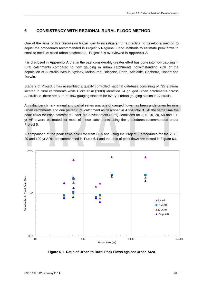
Project 13: Rational Method Developments
P9/S1/005: 12 February 2014 26
0.10
1.00
10.00
10 100 1,000 10,000
Ra
tio
Ura
bn
to
Ru
ral
Pe
ak
Flo
w
Urban Area (ha)
Ratio of Urban to Rural Peak Flow
2 yr ARI
10 yr ARI
20 yr ARI
100 yr ARI
6 CONSISTENCY WITH REGIONAL RURAL FLOOD METHOD
One of the aims of this Discussion Paper was to investigate if it is practical to develop a method to
adjust the procedures recommended in Project 5 Regional Flood Methods to estimate peak flows in
small to medium sized urban catchments. Project 5 is overviewed in Appendix A.
It is disclosed in Appendix A that in the past considerably greater effort has gone into flow gauging in
rural catchments compared to flow gauging in urban catchments notwithstanding 70% of the
population of Australia lives in Sydney, Melbourne, Brisbane, Perth, Adelaide, Canberra, Hobart and
Darwin.
Stage 2 of Project 5 has assembled a quality controlled national database consisting of 727 stations
located in rural catchments while Hicks et al (2009) identified 24 gauged urban catchments across
Australia ie. there are 30 rural flow gauging stations for every 1 urban gauging station in Australia.
An initial benchmark annual and partial series analysis of gauged flows has been undertaken for nine
urban catchments and one paired rural catchment as described in Appendix B. At the same time the
peak flows for each catchment under pre-development (rural) conditions for 2, 5, 10, 20, 50 and 100
yr ARIs were estimated for most of these catchments using the procedures recommended under
Project 5.
A comparison of the peak flows calculate from FFA and using the Project 5 procedures for the 2, 10,
20 and 100 yr ARIs are summarised in Table 6.1 and the ratio of peak flows are plotted in Figure 6.1.
Figure 6-1 Ratio of Urban to Rural Peak Flows against Urban Area
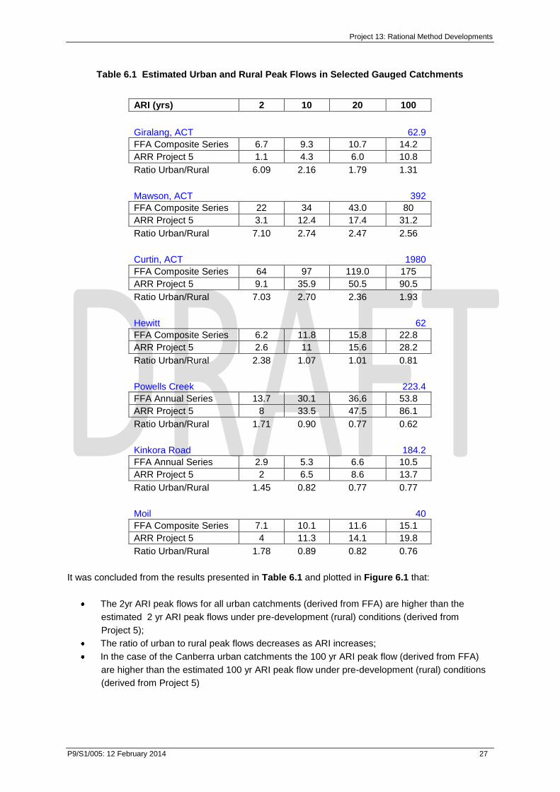
Project 13: Rational Method Developments
P9/S1/005: 12 February 2014 27
Table 6.1 Estimated Urban and Rural Peak Flows in Selected Gauged Catchments
ARI (yrs) 2 10 20 100
Giralang, ACT
62.9
FFA Composite Series 6.7 9.3 10.7 14.2
ARR Project 5 1.1 4.3 6.0 10.8
Ratio Urban/Rural 6.09 2.16 1.79 1.31
Mawson, ACT
392
FFA Composite Series 22 34 43.0 80
ARR Project 5 3.1 12.4 17.4 31.2
Ratio Urban/Rural 7.10 2.74 2.47 2.56
Curtin, ACT
1980
FFA Composite Series 64 97 119.0 175
ARR Project 5 9.1 35.9 50.5 90.5
Ratio Urban/Rural 7.03 2.70 2.36 1.93
Hewitt
62
FFA Composite Series 6.2 11.8 15.8 22.8
ARR Project 5 2.6 11 15.6 28.2
Ratio Urban/Rural 2.38 1.07 1.01 0.81
Powells Creek
223.4
FFA Annual Series 13.7 30.1 36.6 53.8
ARR Project 5 8 33.5 47.5 86.1
Ratio Urban/Rural 1.71 0.90 0.77 0.62
Kinkora Road
184.2
FFA Annual Series 2.9 5.3 6.6 10.5
ARR Project 5 2 6.5 8.6 13.7
Ratio Urban/Rural 1.45 0.82 0.77 0.77
Moil
40
FFA Composite Series 7.1 10.1 11.6 15.1
ARR Project 5 4 11.3 14.1 19.8
Ratio Urban/Rural 1.78 0.89 0.82 0.76
It was concluded from the results presented in Table 6.1 and plotted in Figure 6.1 that:
The 2yr ARI peak flows for all urban catchments (derived from FFA) are higher than the
estimated 2 yr ARI peak flows under pre-development (rural) conditions (derived from
Project 5);
The ratio of urban to rural peak flows decreases as ARI increases;
In the case of the Canberra urban catchments the 100 yr ARI peak flow (derived from FFA)
are higher than the estimated 100 yr ARI peak flow under pre-development (rural) conditions
(derived from Project 5)

Project 13: Rational Method Developments
P9/S1/005: 12 February 2014 28
In the case of the Sydney, Melbourne, and Darwin urban catchments the 100 yr ARI peak flow
(derived from FFA) are lower than the estimated 100 yr ARI peak flow under pre-development
(rural) conditions (derived from Project 5).
It was further concluded that based on the scatter of the calculated ratios of urban to rural peak flows
and the overestimation of rural peak flows in comparison with urban peak flows derived from FFA in
major events in a number of catchments that it is not practical to develop a simple method to adjust
the peak flows from rural catchments to give reliable estimates of peak flows in urban catchments at
this time.

Project 13: Rational Method Developments
P9/S1/005: 12 February 2014 29
7 REFERENCES
Aitken, A.P. (1973) “Hydrologic investigation and design in urban areas - A Review”, AWRC
Technical Paper No 5. Australian Government Publishing Service Canberra
Aitken, A.P. (1975) “Hydrologic investigation and design of urban stormwater drainage systems”,
AWRC Technical Paper No 10. Australian Government Publishing Service Canberra
Black, D.C. and Aitken, A.P. (1977) “Simulation of the urban runoff process”, AWRC Technical Paper
No 26. Australian Government Publishing Service Canberra.
Chapman, T.G. (1968) “Catchment Parameters for a Deterministic Rainfall-Runoff Model in Land
Evaluation”, (ed. G.A. Stewart), MacMillan, Melbourne, pp 312 – 323.
Chapman, T.G. (1970) “Optimization of a Rainfall-Runoff Model for an Arid Catchment”. IASH-
UNESCO Symposium, Wellington, NZ Publication No 96, pp 126 – 124.
City of Canterbury (1995) Stormwater Management Manual – Specification, 9th Edition.
Goyen, A. (1981) “Determination of Rainfall/Runoff Model Parameters”, Thesis submitted for
fulfilment of Master of Engineering, University of technology Sydney.
Goyen, A. (2000) “Spatial and Temporal effects on Urban Rainfall/runoff Modelling”, Thesis submitted
for fulfilment of Doctor of Philosophy, University of Technology Sydney.
Hall, A.G. and Kneen, T.H, (1973) “Design Temporal Patterns of Storm Rainfall in Australia”,
Proceedings, Hydrology Symposium, Engineers Australia, Perth, August, pp 77 – 84.
Hicks, B., Grey, S. and Ball, J. (2009) “A Critical Review of the Urban Rational Method”, Proceedings,
32nd
Hydrology and Water Resources Symposium. Newcastle, November 30 - December 3,
2009, pp 1424 – 1433.
Institution of Engineers Australia (1958) "Australian Rainfall and Runoff", First Report of the
Stormwater Standards Committee of the Institution of Engineers, Australia, 68 pp.
Institution of Engineers Australia (1977) "Australian Rainfall and Runoff Flood Analysis and Design",
IEAust., 159 pp.
Institution of Engineers Australia (1987) "Australian Rainfall and Runoff - A Guide to Flood
Estimation", Editor-in Chief: D.H. Pilgrim, 2 Vols, 374 pp.
Munro, C.H, Vallentine, H.R, and Body, D.N. (1958). “A Method of Design of Urban Storm Drainage
Systems”, Civil Engineering Publication No.5, The University of New South Wales.
Ordon. C. J. (1954) “A Modified Rational Formula for Stormwater Runoff”, Journal of Water and
Sewerage Works.
Phillips, B.C., Lees, S.J. and Lynch, S.J. (1994). “Embedded Design Storms – An Improved
Procedure for Design Flood Level Estimation?” Proceedings, Water Down Under '94, IEAust.,
21-25 November, 1994 Adelaide, pp 235-240.
Pomeroy L, J, M., Swan, R., Thomson, R., Phillips, B., Ball, J., Pathiraja, S. (2013) “Estimation of
imperviousness for a Victorian urban catchment”, Proceedings, 8th Victoria Flood Conference.
February.
Rigby, T., Boyd, M., Roso, S and VanDrie, R (2003) “Storms, Storm Bursts and Flood Estimation - A
need for Review of the ARR Procedures”, Proceedings, 28th International Hydrology and Water
Resources Symposium, 10 - 14 November pp 17 - 24

Project 13: Rational Method Developments
P9/S1/005: 12 February 2014 30
Roso, S. and Rigby, T, (2006). “The Impact of Embedded Design Storms on Flows within a
Catchment”, Proceedings, 30th Hydrology and Water Resources Symposium, 4-7 December
2006, Launceston.
Willing and Partners (1989) Drainage Design Practice for Land Development in the ACT. Part I:
Rational Formula Procedures. National Capital Development Commission, January, 39 pp.
Willing and Partners (1993) Drainage Design Practice Part II: Dept. of Urban Services, ACT City
Services Group, Roads and Transport Branch, Stormwater Section, December, 45 pp + Apps.

APPENDIX A
ARR PROJECT 5 REGIONAL FLOOD METHODS

Project 13: Urban Rational Method Review
P13/S3/001: 12 February 2014 A.1
In Australia, there are many streams where there is little/no recorded streamflow data. In these
ungauged and poorly gauged catchments, there is insufficient information/data to obtain design
flood estimates which are needed to size hydraulic structures, plan and design other water
infrastructure and undertake various environmental and ecological studies. Regional flood
frequency analysis (RFFA) is the most commonly adopted technique to derive design flood estimates
on the ungauged catchments. A RFFA method attempts to transfer flood characteristics
information from a group of gauged catchments to an ungauged catchment of interest. The
RFFA methods recommended in the Australian Rainfall and Runoff (ARR) in 1987 need updating
to reflect the advancements in RFFA methods and new additional streamflow data. To update the
RFFA methods in the ARR, a project team was formed in 2008 and since then the team has been
carrying out research and investigations, which have now formed part of Project 5 „Regional
Flood Methods in Australia in the ARR revision projects.
So far, Stage I and Stage II of Project 5 have been completed.
A.1 PROJECT 5 STAGE 1
The major outcomes of Stage I project were as follows.
Formation of Project 5 team and establishment of contacts and cooperations with various
state agencies to obtain necessary streamflow data and relevant information. About 31
researchers/engineers from over 14 organisations of various Australian states directly
contributed to Project 5 Stage I;
Preparation of initial version of national database which involved examination of a large
number of potential stations from each state, short-listing of the stations, infilling the gaps in
annual maximum flood series, test for outliers, test for trends and test for rating curve
extrapolation error. In Stage I, databases for Victoria, NSW, Qld, Tasmania and SA were
prepared;
Based on detailed literature review, consultation with Project 5 team and various state
representatives and ARR Technical Committee, a number of RFFA methods were selected
for detailed investigation which included the Probabilistic Rational Method, Quantile
Regression Technique and Parameter Regression Technique. For the regression-based
methods, both ordinary least squares and generalised least squares methods were
considered. For the formation of regions, fixed state-based regions and region-of-influence
(based on geographical proximity) were considered.
From initial trend analysis, a good number of stations showed trends in the annual maximum
flood series data; these stations were not included in the development and testing of the
RFFA methods. However, it was decided to conduct further investigation e.g. impact of serial
and cross-correlation on the trends, and relationship between the identified trends and
catchment and climate change/variability indices and impacts of the identified trends on
regional flood estimates with respect to locations and ARIs of the flood estimates.

Project 13: Urban Rational Method Review
P13/S3/001: 12 February 2014 A.2
A.2 PROJECT 5 STAGE 2
The major achievements and/or findings from the Stage II project were as follows.
A quality controlled national database consisting of 727 stations;
That regression-based RFFA methods (such as the quantile regression technique (QRT) or
parameter regression technique (PRT)) are preferable to the Probabilistic Rational Method;
That that Bayesian QRT and Bayesian PRT methods perform very similarly for various
Australian states. Since the PRT method offers several additional advantages over the QRT
(namely, in the PRT flood quantiles increase smoothly with increasing ARIs and from the
regional LP3 distribution, flood quantiles of any ARI (in the range of 2 to 100 years) can be
estimated), this has been recommended for general application in Australia.
From the comparison of fixed regions and region-of-influence (ROI) approaches, it has been
found that, where a region contains a sufficient number of sites, the ROI approach
outperforms the fixed regions. The mean annual flood model generally has the highest model
error as compared to the SD and skew models. However, the SD and skew estimates are
suffered greatly by sampling errors.
The developed RFFA methods in Stage II require data of two or three climatic and physical
catchment characteristics (i.e. catchment area, representative design rainfall intensity and
mean annual rainfall), which are easy to obtain. This would make the application of the
recommended RFFA methods easy and simple.
It has been found that the recommended RFFA methods i.e. GLS-PRT-ROI and GLS-PRT-
fixed region perform quite well for the smaller catchments in the database where there is no
evidence that smaller catchments perform poorly than the medium and larger catchments.
The possibility of extending the RFFA method to very small catchments beyond the limit of
the current Project 5 database has been examined; however, further study is needed to
develop an acceptable method.
The development of a simple Large Flood Regionalisation Model for regional flood estimation
in the major flood range was investigated in Stage I of the project (see Stage I report), which
however did not consider the impacts of inter-station correlation of the annual maximum flood
series among different pairs of stations on final design flood estimates. Some preliminary
investigations on inter-station correlation have been undertaken in this report, which however
needs further investigation.
There is insufficient streamflow data availability at both temporal and spatial scales in the
arid and semi-arid regions of Australia that can be used to develop statistically meaningful
RFFA methods. A simplified index type RFFA is recommended for arid/semi-arid regions of
Australia where four separate regions are recommended at this stage (this needs further
development and testing before inclusion in the ARR).

Project 13: Urban Rational Method Review
P13/S3/001: 12 February 2014 A.3
In the preliminary investigation (see Stage I report), about 13% of the selected stations (for Project 5)
showed a trend in the annual maximum flood series data. In the Stage II report, the impacts of
serial and cross-correlation on trend analysis have been investigated. At the significance level of
10% and with the consideration of the cross-correlation among the sites in the network, the field
significance of downward trends in the annual maximum flood series was detected over the whole
country. However, the field significance of upward trends was discovered to be statistically non-
significant at 10% significant level. The impacts of the identified trends on regional flood quantile
estimates for ARIs in the range of 2 to 100 years will be investigated in Stage III of the project. This is
expected to produce climate change adjustment factors as a function of ARIs and locations across
Australia.
The testing of the recommended RFFA methods for Australia by various states/stakeholders in
cooperation with the Project 5 team has been recommended. A set of future tasks has been
identified. Also, the scope of developing an application tool/software has been indicated.
Stage II developed a firm basis for recommendations on the RFFA methods to be included in the
revised ARR Chapter (4th
edition). It has also identified future research and development work in
Stage III of the Project, required to develop the Stage II findings into a final set of methods, design
databases, user guidelines and application tools.
The results presented in this report are applicable to the rural catchments in the vicinity of the catchments
selected in this study; this should not be applied to urban catchments.
APPENDIX B
FLOOD FREQUENCY ANALYSIS IN SELECTED GAUGED URBAN CATCHMENTS

Project 9: Urban Drainage System Hydraulics
P9/S1/005: 12 February 2014 B.1
B.1 DISPARITY BETWEEN NUMBER OF RURAL AND URBAN GAUGED CATCHMENTS
It is apparent from a comparison of the discussion in Section 3 and Appendix A that in the past
considerably greater effort has gone into flow gauging in rural catchments compared to flow gauging
in urban catchments notwithstanding 70% of the population of Australia lives in Sydney, Melbourne,
Brisbane, Perth, Adelaide, Canberra, Hobart and Darwin.
Stage 2 of Project 5 has assembled a quality controlled national database consisting of 727 stations
located in rural catchments while Hicks et al (2009) identified 24 gauged urban catchments across
Australia ie. there are 30 rural flow gauging stations for every 1 urban gauging station in Australia.
The length of record at stations in urban catchments is also often restricted to 10 years or less.
As disclosed by Hicks et al (2009) the number of urban catchments (500 ha or less) with 20
years of records is only 11, with 30 years of record is 7, with 40 years of record is 4 and with 50
years record is 1 only.
The length of record can have a significant effect on the flood frequency curve.
When developing and testing a rainfall-runoff estimation procedure including a simple statistical
form of the Rational Formula, the flood frequency curve derived from gauged flows or individual
peak flow quantiles are the objective function.
Even if the quality of the gauged data is of a very high standard and the annual maximum peaks
as well as any additional significant peak values are judged to be of high accuracy, this does not
mean that the flood frequency curve calculated using a limited record length will be accurate
over the full range of AEPs eg. up to 1% AEP.
B.2 FLOOD FREQUENCY ANALYSIS
The updating of the Rational Formula method to reduce the potential error levels in the peak flows
estimated using the procedure and/or to improve the guidance on rainfall-runoff model parameters for
urban catchments can only occur if there is a flood frequency curve available for the gauged
catchment to provide the benchmark against which peak flow predictions can be tested in accordance
with the approaches adopted in the Part I and Part II studies conducted in the ACT (Willing &
Partners, 1989 and 1993). These studies are attached in Appendix E and F respectively.
In the 1987 edition of ARR, Chapter 10 on flood frequency analysis extensively discusses the
methodology, limitations and qualifications associated with estimating a flood frequency curve
from data of varying quality, inclusive outliers, and record length. The roles of partial and annual
series in flood frequency analysis is described. The importance of the partial series is explained
particularly when considering the frequent floods of say less than 10% AEP.
An initial benchmark has been created for nine urban catchments and one paired rural
catchment based on annual and partial series analysis of gauged flows for each urban
catchment. The catchments that have been analysed are summarised in Table B.1.
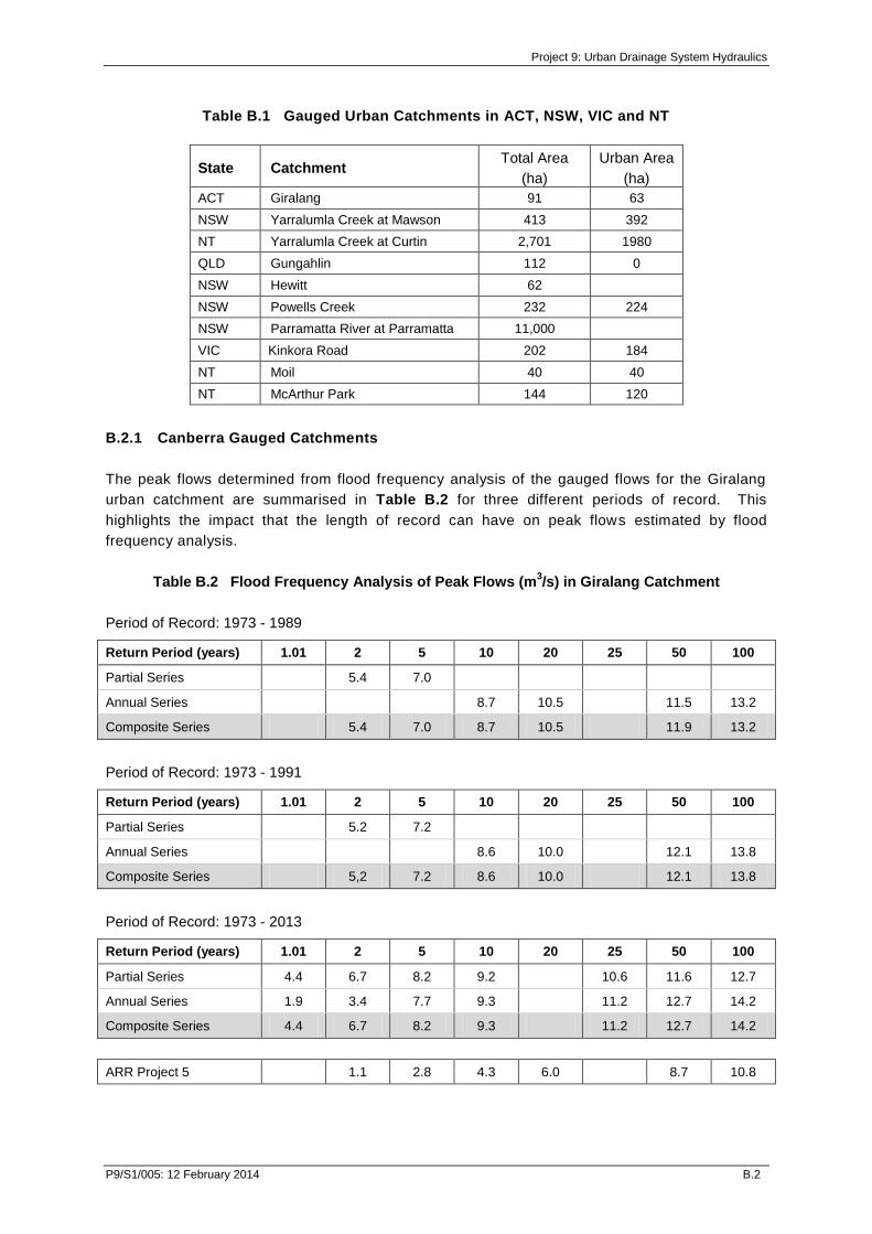
Project 9: Urban Drainage System Hydraulics
P9/S1/005: 12 February 2014 B.2
Table B.1 Gauged Urban Catchments in ACT, NSW, VIC and NT
State Catchment Total Area
(ha)
Urban Area
(ha)
ACT Giralang 91 63
NSW Yarralumla Creek at Mawson 413 392
NT Yarralumla Creek at Curtin 2,701 1980
QLD Gungahlin 112 0
NSW Hewitt 62
NSW Powells Creek 232 224
NSW Parramatta River at Parramatta 11,000
VIC Kinkora Road 202 184
NT Moil 40 40
NT McArthur Park 144 120
B.2.1 Canberra Gauged Catchments
The peak flows determined from flood frequency analysis of the gauged flows for the Giralang
urban catchment are summarised in Table B.2 for three different periods of record. This
highlights the impact that the length of record can have on peak flows estimated by flood
frequency analysis.
Table B.2 Flood Frequency Analysis of Peak Flows (m3/s) in Giralang Catchment
Period of Record: 1973 - 1989
Return Period (years) 1.01 2 5 10 20 25 50 100
Partial Series 5.4 7.0
Annual Series 8.7 10.5 11.5 13.2
Composite Series 5.4 7.0 8.7 10.5 11.9 13.2
Period of Record: 1973 - 1991
Return Period (years) 1.01 2 5 10 20 25 50 100
Partial Series 5.2 7.2
Annual Series 8.6 10.0 12.1 13.8
Composite Series 5,2 7.2 8.6 10.0 12.1 13.8
Period of Record: 1973 - 2013
Return Period (years) 1.01 2 5 10 20 25 50 100
Partial Series 4.4 6.7 8.2 9.2 10.6 11.6 12.7
Annual Series 1.9 3.4 7.7 9.3 11.2 12.7 14.2
Composite Series 4.4 6.7 8.2 9.3 11.2 12.7 14.2
ARR Project 5 1.1 2.8 4.3 6.0 8.7 10.8

Project 9: Urban Drainage System Hydraulics
P9/S1/005: 12 February 2014 B.3
Table B.3 Flood Frequency Analysis of Peak Flows (m3/s) in
Yarralumla Creek Catchment at Mawson
Period of Record: 1971 - 1992
Return Period (years) 1.01 2 5 10 20 25 50 100
Partial Series 22 29 34 42 47 53
Annual Series 18 28 35 45 53 61
Composite Series 22 29 34 43 50 63 80
ARR Project 5 3.1 8.0 12.4 17.4 24.9 31.2
The peak flows determined from flood frequency analysis of the gauged flows for the Yarralumla
Creek catchment at Mawson are summarised in Table B.3. The 2, 5 and 10 yr ARI values in the
composite series were based on a LP3 partial series analysis. The 20, 25, 50 and 100 yr ARI peak
flows in the composite series were scaled off a graph with the highest (outlier) peak flow of 195 m3/s
recorded in the 1971 flood plotted at an estimated position of 1,000 year ARI.
The peak flows determined from flood frequency analysis of the gauged flows for the Yarralumla
Creek catchment at Curtin are summarised in Table B.4. The 2, 5 and 10 yr ARI values in the
composite series were based on a LP3 partial series analysis. The 20, 25, 50 and 100 yr ARI peak
flows in the composite series were scaled off a graph with the highest (outlier) peak flow of 240 m3/s
recorded in the 1971 flood plotted at an estimated position of 350 year ARI.
The peak flows determined from flood frequency analysis of the gauged flows for the Gungahlin
rural catchment are summarised in Table B.5.
Table B.4 Flood Frequency Analysis of Peak Flows (m3/s) in
Yarralumla Creek Catchment at Curtin
Period of Record: 1970 - 1992
Return Period (years) 1.01 2 5 10 20 25 50 100
Partial Series 64 83 97 118 135 154
Annual Series 54 76 93 115 135 156
Composite Series 64 83 97 119 125 150 175
ARR Project 5 9.1 23.1 35.9 50.5 72.3 90.5
Table B.5 Flood Frequency Analysis of Peak Flows (m3/s) in Gungahlin Catchment
Period of Record: 1973 - 1991
Return Period (years) 1.01 2 5 10 20 25 50 100
Partial Series 0.25 0.90 1.6 2.3 3.3 4.3 5.5
Annual Series 0.03 0.46 1.2 1.9 3.0 4.1 5.4
Composite Series 0.25 0.90 1.6 1.9 3.0 4.1 5.4
ARR Project 5 1.5 3.8 6.0 8.4 12.0 15.0

Project 9: Urban Drainage System Hydraulics
P9/S1/005: 12 February 2014 B.4
B.2.2 Sydney Gauged Urban Catchments
The estimated peak flows for the Hewitt catchment are summarised in Table B.6. The estimated
series is based on the results from catchment simulation as described in Appendix D.
Table B.6 Estimated Peak Flows (m3/s) in Hewitt Catchment
Period of Record: 1993 - 1995
Return Period (years) 1.01 2 5 10 20 25 50 100
Partial Series
Annual Series
Estimated Series 4.5 6.2 10.1 11.8 15.8 18.3 22.8
ARR Project 5 2.6 7.0 11.0 15.6 22.5 28.2
The peak flows determined from flood frequency analysis of the gauged flows for the Powells
Creek catchment are summarised in Table B.7. At the time of preparation of this Discussion Paper
only the annual series results were available. The slope of the annual series flood frequency curve is
significantly flatter than the curve for the Parramatta River at Parramatta (refer Table B.8).
The peak flows determined from flood frequency analysis of the gauged flows for the Parramatta
River catchment at Parramatta are summarised in Table B.8. No data was available for partial
series over the period 1979 – 2000. The highest peak on record over the 21 years of record was
781 m3/s during the 1988 flood. It is likely that if the partial series analysis over the same period
was included the peak flows for floods less than 10 year ARI would be higher. It is also likely
that the 100 yr ARI peak flow could decrease significantly as the length of record increases.
Table B.7 Flood Frequency Analysis of Peak Flows (m3/s) in the Powells Creek Catchment
Period of Record: 1973 - 1989
Return Period (years) 1.01 2 5 10 20 25 50 100
Partial Series
Annual Series 4.4 13.7 23.9 30.1 36.6 46.0 53.8
Composite Series
ARR Project 5 8.0 21.2 33.5 47.5 68.5 86.1
Table B.8 Flood Frequency Analysis of Peak Flows (m3/s) in the
Parramatta River Catchment at Parramatta
Period of Record: 1979 - 2000
Return Period (years) 1.01 2 5 10 20 25 50 100
Partial Series
Annual Series 25 130 293 469 710 1,165 1,647
Composite Series
ARR Project 5 76 202 318 451 651 818

Project 9: Urban Drainage System Hydraulics
P9/S1/005: 12 February 2014 B.5
Probability
0.9999 0.999 0.99 0.9 0.5 0.2 0.1 0.02 0.005 0.001 0.0001
Return Period
1.0 1.1 2 5 10 50 200 1000 10000
nu
ll in
UN
SP
EC
IF
1.0
10.0
100.0
General Frequency Analytical Plot for kink
Computed Curve Expected Probability Curve
5 Percent Confidence Limit 95 Percent Confidence Limit
Observed Events (Weibull plotting positions) High Outlier
Probability
0.9999 0.999 0.99 0.9 0.5 0.2 0.1 0.02 0.005 0.001 0.0001
Return Period
1.0 1.1 2 5 10 50 200 1000 10000
nu
ll in
UN
SP
EC
IF
1.0
10.0
100.0
General Frequency Analytical Plot for kink
Computed Curve Expected Probability Curve
5 Percent Confidence Limit 95 Percent Confidence Limit
Observed Events (Weibull plotting positions) Low Outlier
B.2.3 Melbourne Gauged Urban Catchment
Rainfall and streamflow records spanned 35 years (1977 to 2012) in six-minute intervals at the
Kinkora Road Retarding Basin (Gauge Station 229636A). The retarding basin located at the base of
the catchment is not included within the catchment boundary and the inflows to the station are not
influenced by the retarding basin (Pomeroy et al, 2013). An analysis of the peak flows recorded in the
Kinkora Road urban catchment was undertaken using HEC-SSP.
Figure B.1 Flood Frequency Curve for Kinkora Road Catchment including 1997 Outlier
Figure B.2 Flood Frequency Curve for Kinkora Road Catchment with
2.5 m3/s substituted for 1977 Outlier

Project 9: Urban Drainage System Hydraulics
P9/S1/005: 12 February 2014 B.6
The analysis presented in Figure B.1 highlighted that the peak flow of 19.69 m3/s recorded in 1977 is
an outlier. A review of the gauged flow records found that a peak flow of 19.69 m3/s was recorded at
four separate times during the same event. These peak flows were recorded at 15:16 hours on 27
July 1977 at, at 18:48 hours on 29 July1977, at 00:06 hours on 30 July 1977 and at 04:48 hours on 30
July 1977. A review of the rainfall data for the same period disclosed that there was only low rainfall
of several millimetres was recorded. Additionally many data crashes were observed during this event.
The peak flow of 5.92 m3/s recorded in 1984 was also examined. In this instance recorded flow event
aligned with in excess of 20 mm of rainfall immediately prior to the recorded peak flow. It was
concluded that this observed rainfall and runoff in 1984 was consistent and that the recorded peak
flows in July 1977 were not supported by the rainfall record and are highly suspect.
The peak flows were re-analysed based on substituting a nominal peak flow of 2.5 m3/s for the 1977
event and gave the flood frequency curve presented in Figure B.2. This is the annual series reported
in Table B.9.
The peak flows determined from flood frequency analysis of the gauged flows for the Kinkora
Road catchment are summarised in Table B.9. It is likely that if the partial series analysis over
the same period was included the peak flows for floods less than 10 year ARI would be higher.
Table B.9 Flood Frequency Analysis of Peak Flows (m3/s) in the Kinkora Road Catchment
Period of Record: 1977 - 2012
Return Period (years) 1.01 2 5 10 20 25 50 100
Partial Series
Annual Series 1.8 2.9 4.2 5.3 6.6 8.6 10.5
Composite Series
ARR Project 5 2.0 4.5 6.5 8.6 11.5 13.7
B.2.4 Darwin Gauged Urban Catchments
The peak flows determined from flood frequency analysis of the gauged flows for the Moil urban
catchment are summarised in Table B.10. In this analysis the partial series analysis was
approximated by an analysis of monthly peak flows. A peak over threshold style approach was
adopted by selecting only monthly peaks within a year that exceeded a certain threshold. This
threshold was selected so that there was the same number of peak flows as there were years.
Table B.10 Flood Frequency Analysis of Peak Flows (m3/s) in the Moil Catchment
Period of Record: 1984 - 2010
Return Period (years) 1.01 2 5 10 20 25 50 100
Partial Series 4.43 7.1 8.9 10.1
Annual Series 1.83 5.8 8.4 10.1 11.6 13.6 15.1
Composite Series 4.43 7.1 8.9 10.1 11.6 13.6 15.1
ARR Project 5 4.0 8.3 11.3 14.1 17.4 19.8
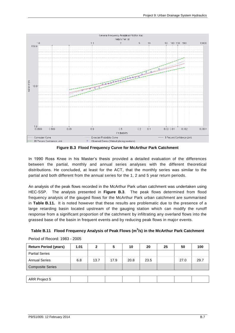
Project 9: Urban Drainage System Hydraulics
P9/S1/005: 12 February 2014 B.7
Figure B.3 Flood Frequency Curve for McArthur Park Catchment
In 1990 Ross Knee in his Master’s thesis provided a detailed evaluation of the differences
between the partial, monthly and annual series analyses with the different theoretical
distributions. He concluded, at least for the ACT, that the monthly series was similar to the
partial and both different from the annual series for the 1, 2 and 5 year return periods.
An analysis of the peak flows recorded in the McArthur Park urban catchment was undertaken using
HEC-SSP. The analysis presented in Figure B.3. The peak flows determined from flood
frequency analysis of the gauged flows for the McArthur Park urban catchment are summarised
in Table B.11. It is noted however that these results are problematic due to the presence of a
large retarding basin located upstream of the gauging station which can modify the runoff
response from a significant proportion of the catchment by infiltrating any overland flows into the
grassed base of the basin in frequent events and by reducing peak flows in major events.
Table B.11 Flood Frequency Analysis of Peak Flows (m3/s) in the McArthur Park Catchment
Period of Record: 1983 - 2005
Return Period (years) 1.01 2 5 10 20 25 50 100
Partial Series
Annual Series 6.8 13.7 17.9 20.8 23.5 27.0 29.7
Composite Series
ARR Project 5

APPENDIX C
PRELIMINARY PART I STUDY – CANBERRA, SYDNEY, MELBOURNE, DARWIN

Project 9: Urban Drainage System Hydraulics
P9/S1/005: 12 February 2014 C.1
C.1 BACKGROUND
The 1987edition of ARR recommended changes to both the estimation of both time of concentration
and runoff coefficient in urban drainage design. 1987 ARR departed from the empirical relationship
given in Equation 2. Instead, it recommended the use of the "kinematic wave" equation for overland
flow time previously described by Ragan & Duru (1972). The 1987 ARR varies from the 1958 and
1977 editions in its presentation of runoff coefficients for design purposes. This edition presents a:
"composite relationship reflecting experience of drainage authorities and evidence from
the few gauged urban catchments with suitable lengths of record ..."
During the consultation period held prior to the release of 1987 ARR a study was carried out in the
ACT at the request of the ACT Government to review the possible effects of differences between the
urban Rational Method procedures as recommended in 1977 ARR and 1987 ARR. This review is
described in a report titled “Drainage Design Practice for Land Development in the ACT. Part I:
Rational Formula Procedures”, Willing and Partners (1989) which is attached in Appendix E.
This report ultimately recommended a semi-probabilistic based procedure for urban drainage design
undertaken using the Rational Method in the ACT. The recommended procedure was based on the
outcomes of testing different combinations of the 1977 and 1987 procedures for estimating runoff
coefficient and time of concentration for estimating runoff coefficient to estimate flow peak quantiles in
two gauged urban catchments. The estimated flow quantiles were then compared with peak flows
determined using a flood frequency analysis. It was found that the combination of the procedures for
estimating runoff coefficient and time of concentration given in the 1977 ARR best fitted the flood
frequency curves from 2 yr ARI to 100 yr ARI.
Since the publication of 1987 ARR a number of water authorities as well as Councils have also
published their own recommendations for how the Rational Formula should be applied to urban
catchments in their jurisdiction. Typically these guidelines recommend procedures for estimating
runoff coefficient and time of concentration which differ from those recommended in the 1987 ARR.
Since 1989 additional data has been collected in the Giralang catchment which has allowed the
updating of the 1987 analysis as well as the preliminary testing of the sensitivity of the predicted peak
flows to characterising a catchment based on total impervious area (TIA) or effective impervious area
(EIA) as assessed in ARR Project 6 Stage 2 - Analysis of Effective Impervious Area & Pilot Study of
Losses in Urban Catchments.
C.2 CANBERRA
The Giralang catchment assessment was updated based on the following catchment properties.
Catchment Year Total Area*
(TA) (ha)
Urban Area^
(UA) (ha)
Total Impervious
Area* (TIA) (ha)
Effective Impervious
Area# (EIA) (ha)
Giralang 1990 90.74 62.9 19.8
Giralang 2013 90.98 61.8 28.4 21.0 – 22.7
*Determined using the desktop GIS method
^The Urban Area is classified as the total developed area excluding large open space #EIA varies based on rainfall gauge adopted for analysis in period 1973 - 2012

Project 9: Urban Drainage System Hydraulics
P9/S1/005: 12 February 2014 C.2
Table C.1
Adopted Design IFD parameters for the Giralang Catchment
Parameter Value
2 Year ARI 1 hour Intensity 22.0 mm/hr
2 Year ARI 12 hour Intensity 4.3 mm/hr
2 Year ARI 72 hour Intensity 1.14 mm/hr
50 Year ARI 1 hour Intensity 43.0 mm/hr
50 Year ARI 12 hour Intensity 8.0 mm/hr
50 Year ARI 72 hour Intensity 2.25 mm/hr
Location Skew 0.24
F2 4.28
F50 15.55
The adopted IFD parameter values are given in Table C.1.
In the case of assessment undertaken using the 1977 ARR runoff coefficients the adopted runoff
coefficient curve number was No. 4 (refer Figure 2.3)
The overland flow time was calculated using the following equation (S.I. units):
to = 107 n L0.333
(C.1)
S0.2
where to = overland flow travel time (minutes)
L = flow path length (m)
n = Horton's roughness value for the surface
S = slope of surface (%)
The adopted parameter values for assessment purposes were:
L = 50 m
n = 0.015 for impervious surfaces
n = 0.04 for pervious surfaces
S = 4.5 %
Giving to = 15.7 mins for pervious surfaces including an estimated 4 mins travel
time
to = 8.4 mins for impervious surfaces including an estimated 4 mins travel
time
In the case of the 1987 ARR procedures, runoff coefficients were estimated using Equations 4, 5 and
6 (refer Section 2).
1987 ARR recommended the use of the "kinematic wave" equation for overland flow time previously
described by Ragan & Duru (1972). This equation is as follows:
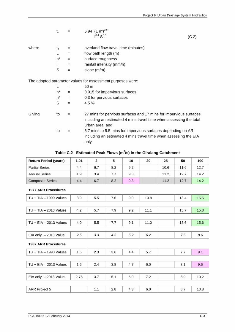
Project 9: Urban Drainage System Hydraulics
P9/S1/005: 12 February 2014 C.3
to = 6.94 (L n*)0.6
I0.4
S0.3
(C.2)
where to = overland flow travel time (minutes)
L = flow path length (m)
n* = surface roughness
I = rainfall intensity (mm/h)
S = slope (m/m)
The adopted parameter values for assessment purposes were:
L = 50 m
n* = 0.015 for impervious surfaces
n* = 0.3 for pervious surfaces
S = 4.5 %
Giving to = 27 mins for pervious surfaces and 17 mins for impervious surfaces
including an estimated 4 mins travel time when assessing the total
urban area; and
to = 6.7 mins to 5.5 mins for impervious surfaces depending on ARI
including an estimated 4 mins travel time when assessing the EIA
only
Table C.2 Estimated Peak Flows (m3/s) in the Giralang Catchment
Return Period (years) 1.01 2 5 10 20 25 50 100
Partial Series 4.4 6.7 8.2 9.2 10.6 11.6 12.7
Annual Series 1.9 3.4 7.7 9.3 11.2 12.7 14.2
Composite Series 4.4 6.7 8.2 9.3 11.2 12.7 14.2
1977 ARR Procedures
TU + TIA – 1990 Values 3.9 5.5 7.6 9.0 10.8 13.4 15.5
TU + TIA – 2013 Values 4.2 5.7 7.9 9.2 11.1 13.7 15.8
TU + EIA – 2013 Values 4.0 5.5 7.7 9.1 11.0 13.6 15.6
EIA only – 2013 Value 2.5 3.3 4.5 5.2 6.2 7.5 8.6
1987 ARR Procedures
TU + TIA – 1990 Values 1.5 2.3 3.6 4.4 5.7 7.7 9.1
TU + EIA – 2013 Values 1.6 2.4 3.8 4.7 6.0 8.1 9.6
EIA only – 2013 Value 2.78 3.7 5.1 6.0 7.2 8.9 10.2
ARR Project 5 1.1 2.8 4.3 6.0 8.7 10.8

Project 9: Urban Drainage System Hydraulics
P9/S1/005: 12 February 2014 C.4
The peak flows reported in Table C.2 were estimated using a single node xprathgl model of the
Giralang catchment.
It was concluded from a comparison of the various results that:
The 1977 ARR procedures give peak flows which match the peak flows adopted for the
composite series based on flood frequency analysis (FFA) except for flows based on EIA only;
The 1987 procedures give peak flows lower than the peak flows adopted for the composite
series based on flood frequency analysis with the estimated 100 yr ARI peak flow comparable
to the 10 yr ARI peak flow from the FFA;
For 10 yr ARI and above the 1987 ARR procedures give similar peak flows to the ARR Project
5 procedures for rural catchments.
C.3 SYDNEY
The Hewitt catchment assessment was based on the following catchment properties.
Catchment Year Total Area
(TA) (ha)
Urban Area
(UA) (ha)
Total Impervious
Area* (TIA) (ha)
Effective Impervious
Area (EIA) (ha)
Hewitt 2013 62.0 62.0 19.8
Table C.3
Adopted Design IFD parameters for the Powells Creek Catchment
Parameter Value
2 Year ARI 1 hour Intensity 29.69 mm/hr
2 Year ARI 12 hour Intensity 6.53 mm/hr
2 Year ARI 72 hour Intensity 1.89 mm/hr
50 Year ARI 1 hour Intensity 59.06 mm/hr
50 Year ARI 12 hour Intensity 12.79 mm/hr
50 Year ARI 72 hour Intensity 4.32 mm/hr
Location Skew 0.02
F2 4.3
F50 15.8
The adopted IFD parameter values are given in Table C.3.
In the case of assessment undertaken using the 1977 ARR runoff coefficients the adopted runoff
coefficient curve number was No. 4 (refer Figure 2.3).
For 1977 ARR procedures the adopted parameter values for assessment of time of concentration
were:
L = 50 m
n = 0.015 for impervious surfaces
n = 0.04 for pervious surfaces
S = 2.5 %
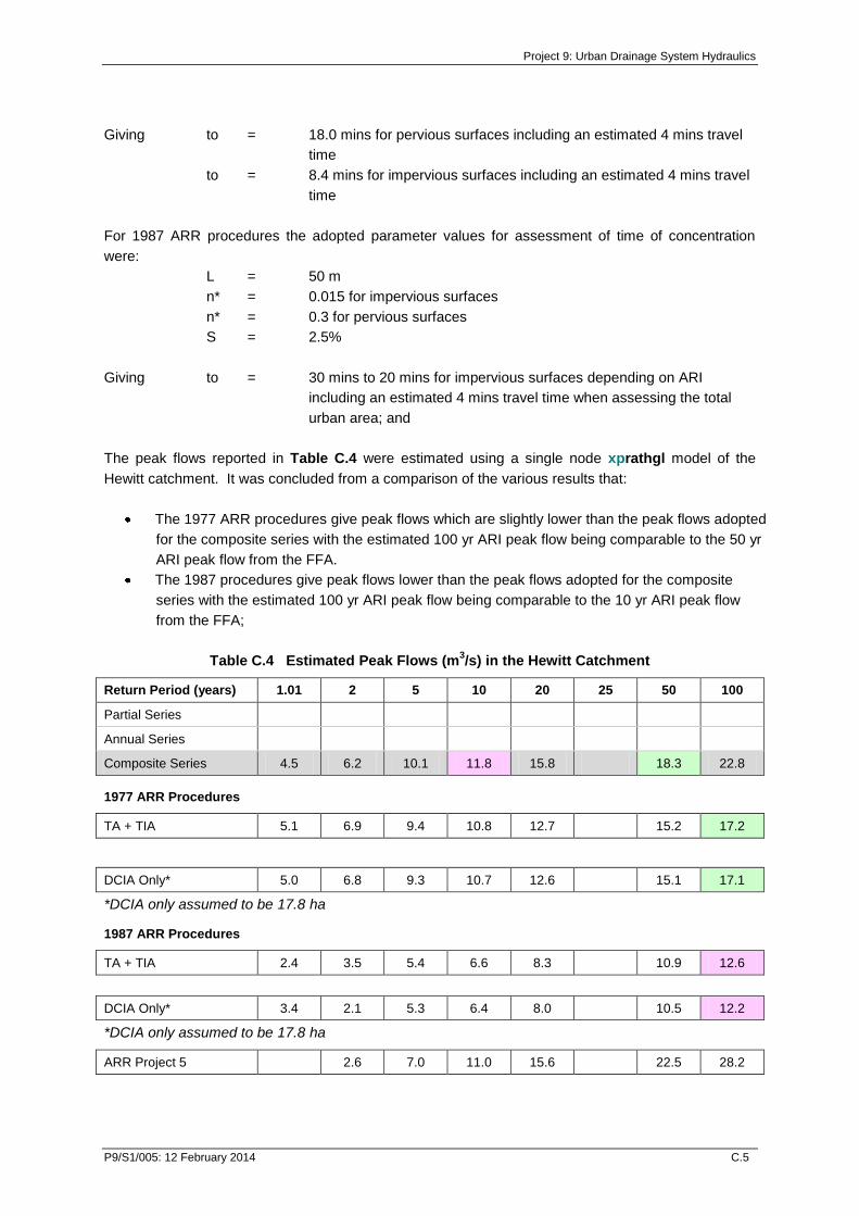
Project 9: Urban Drainage System Hydraulics
P9/S1/005: 12 February 2014 C.5
Giving to = 18.0 mins for pervious surfaces including an estimated 4 mins travel
time
to = 8.4 mins for impervious surfaces including an estimated 4 mins travel
time
For 1987 ARR procedures the adopted parameter values for assessment of time of concentration
were:
L = 50 m
n* = 0.015 for impervious surfaces
n* = 0.3 for pervious surfaces
S = 2.5%
Giving to = 30 mins to 20 mins for impervious surfaces depending on ARI
including an estimated 4 mins travel time when assessing the total
urban area; and
The peak flows reported in Table C.4 were estimated using a single node xprathgl model of the
Hewitt catchment. It was concluded from a comparison of the various results that:
The 1977 ARR procedures give peak flows which are slightly lower than the peak flows adopted
for the composite series with the estimated 100 yr ARI peak flow being comparable to the 50 yr
ARI peak flow from the FFA.
The 1987 procedures give peak flows lower than the peak flows adopted for the composite
series with the estimated 100 yr ARI peak flow being comparable to the 10 yr ARI peak flow
from the FFA;
Table C.4 Estimated Peak Flows (m3/s) in the Hewitt Catchment
Return Period (years) 1.01 2 5 10 20 25 50 100
Partial Series
Annual Series
Composite Series 4.5 6.2 10.1 11.8 15.8 18.3 22.8
1977 ARR Procedures
TA + TIA 5.1 6.9 9.4 10.8 12.7 15.2 17.2
DCIA Only* 5.0 6.8 9.3 10.7 12.6 15.1 17.1
*DCIA only assumed to be 17.8 ha
1987 ARR Procedures
TA + TIA 2.4 3.5 5.4 6.6 8.3 10.9 12.6
DCIA Only* 3.4 2.1 5.3 6.4 8.0 10.5 12.2
*DCIA only assumed to be 17.8 ha
ARR Project 5 2.6 7.0 11.0 15.6 22.5 28.2

Project 9: Urban Drainage System Hydraulics
P9/S1/005: 12 February 2014 C.6
The Powells Creek catchment assessment was based on the following catchment properties.
Catchment Year Total Area*
(TA) (ha)
Urban Area^
(UA) (ha)
Total Impervious
Area* (TIA) (ha)
Effective Impervious
Area# (EIA) (ha)
Powells Creek 1990 234 223.4 117.0
Powells Creek 2013 231.9 223.4 151.7 90.6 – 95.1
*Determined using the desktop GIS method
^The Urban Area is classified as the total developed area excluding large open space #EIA based on analysis in period 1973 - 1989
Table C.5
Adopted Design IFD parameters for the Powells Creek Catchment
Parameter Value
2 Year ARI 1 hour Intensity 34.45 mm/hr
2 Year ARI 12 hour Intensity 7.31 mm/hr
2 Year ARI 72 hour Intensity 2.41 mm/hr
50 Year ARI 1 hour Intensity 65.94 mm/hr
50 Year ARI 12 hour Intensity 15.53 mm/hr
50 Year ARI 72 hour Intensity 5.04 mm/hr
Location Skew 0.0
F2 4.3
F50 18.84
The adopted IFD parameter values are given in Table C.5.
In the case of assessment undertaken using the 1977 ARR runoff coefficients the adopted runoff
coefficient curve number was No. 5 (refer Figure 2.3)
For 1977 ARR procedures the adopted parameter values for assessment of time of concentration
were:
L = 50 m
n = 0.015 for impervious surfaces
n = 0.04 for pervious surfaces
S = 1 %
Giving to = 22.7 mins for pervious surfaces including an estimated 7 mins travel
time
to = 12.9 mins for impervious surfaces including an estimated 7 mins
travel time

Project 9: Urban Drainage System Hydraulics
P9/S1/005: 12 February 2014 C.7
For 1987 ARR procedures the adopted parameter values for assessment of time of concentration
were:
L = 50 m
n* = 0.015 for impervious surfaces
n* = 0.3 for pervious surfaces
S = 1 %
Giving to = 40 mins for pervious surfaces and 27 mins for impervious surfaces
including an estimated 7 mins travel time when assessing the total
urban area; and
to = 11 mins to 9 mins for impervious surfaces depending on ARI
including an estimated 7 mins travel time when assessing the EIA
only.
The peak flows reported in Table C.6 were estimated using a single node xprathgl model of the
Powells Creek catchment.
Table C.6 Estimated Peak Flows (m3/s) in the Powells Creek Catchment
Return Period (years) 1.01 2 5 10 20 25 50 100
Partial Series
Annual Series 4.4 13.7 23.9 30.1 36.6 46.0 53.8
Composite Series
1977 ARR Procedures
TA + TIA – 1990 Values 19.9 26.5 35.0 39.5 45.9 54.2 60.6
TU + DCIA Road Only* – 2013 Values
15.7 21.7 29.5 33.7 39.7 47.6 53.6
*DCIA Road only estimated to be 42 ha
TA + EIA# 18.9 25.4 33.7 38.2 44.5 52.7 59.0
#EIA assumed to be 100 ha
EIA only # 14.9 19.0 24.3 27.0 31.0 36.0 39.8
#EIA assumed to be 100 ha
1987 ARR Procedures
TA + TIA – 1990 Values 11.6 16.7 25.2 30.3 37.5 48.1 55.0
TA + EIA# 11.0 15.9 23.9 28.7 35.5 45.7 52.4
#EIA assumed to be 100 ha
EIA only # 16.1 21.0 27.1 30.4 35.0 41.0 45.5
#EIA assumed to be 100 ha
ARR Project 5 8.0 21.2 33.5 47.5 68.5 86.1

Project 9: Urban Drainage System Hydraulics
P9/S1/005: 12 February 2014 C.8
C.3 MELBOURNE
Melbourne Water provides guidelines on the application of the Rational Method in urban catchments
as follows.
The Rational Method is generally used to calculate design peak flow rates throughout the
pipeline drainage system, provided the drainage catchment is less than 400 hectares. The
method does not allow for flood storage effects. Therefore, when there are or will be retarding
basins in the system, suitable adjustments must be made for the basin outflows, or an
alternative method that provides for flood storage effects must be used.
The Rational Method is described in Book 8 of Australian Rainfall and Runoff. ……
The following guidelines are provided for use of the Rational Method, including values that
Melbourne Water requires to be used:
1. The downstream design peak flow rate should not be less than the upstream flow rate
for a piped system
2. Partial area effects should be considered in the design (refer Australian Rainfall and
Runoff Book 8 for guidance)
3. The applicable average recurrence interval, runoff coefficient, area of catchment and
design average rainfall intensity will be determined as shown below.
Table 1 below presents a range of coefficients to be applied to various land use. The values
presented are slightly higher than the values that would be obtained by following the method
prescribed by ARR. They contain adjustments to suit Melbourne's conditions and must be used
in preference to the ARR values.
Table 1 Runoff Coefficients
Land Use C (5 Year ARI) C (100 Year ARI)
Major open space 0.20 0.30
Residential (avg lot size):
4000 m2 0.30 0.40
750 m2 0.40 0.50
500 m2 0.50 0.65
350 m2 0.60 0.75
< 350 m2 0.70 to 0.90 0.9
Major road reserves 0.50 to 0.80 0.65 to 0.9
Commercial/industrial 0.70 to 0.90 0.9
If different ARIs are required, and for situations in which there are a range in values in the table,
or where the proposed land use is different to that prescribed, the fraction impervious must be
estimated and taken into consideration. In such instances the method prescribed by ARR
Book 8 should be followed.
The time of concentration at a particular location is generally the time required for runoff to
travel by the longest available flowpath to that location.

Project 9: Urban Drainage System Hydraulics
P9/S1/005: 12 February 2014 C.9
In many cases however a "partial area" affect occurs through the lower part of the catchment,
where flows are higher than those calculated for the entire catchment, because the time of
concentration is lower and the design rainfall intensity is higher.
The method prescribed by 1998 ARR Book 8 is exactly the same as the method detailed in
Chapter 14 of 1987 ARR.
The Kinkora Road catchment assessment was based on the following catchment properties.
Catchment Year Total Area*
(TA) (ha)
Urban Area^
(UA) (ha)
Total Impervious
Area* (TIA) (ha)
Effective Impervious
Area# (EIA) (ha)
Kinkora Road 202.1 184.2 121.9 72.3 ha
*Determined using the desktop GIS method
^The Urban Area is classified as the total developed area excluding large open space
#EIA based on analysis of period 1977 - 2012
Table C.7
Adopted Design IFD parameters for the Kinkora Road Catchment
Parameter Value
2 Year ARI 1 hour Intensity 19.12 mm/hr
2 Year ARI 12 hour Intensity 4.22 mm/hr
2 Year ARI 72 hour Intensity 1.23 mm/hr
50 Year ARI 1 hour Intensity 37.42 mm/hr
50 Year ARI 12 hour Intensity 7.25 mm/hr
50 Year ARI 72 hour Intensity 2.30 mm/hr
Location Skew 0.36
F2 4.28
F50 14.97
The adopted IFD parameter values are given in Table C.7.
In the case of assessment undertaken using the 1977 ARR runoff coefficients the adopted runoff
coefficient curve number was No. 4 (refer Figure 2.3).
For 1977 ARR procedures the adopted parameter values for assessment of time of concentration
were:
L = 50 m
n = 0.015 for impervious surfaces
n = 0.04 for pervious surfaces
S = 1.8 %
Giving to = 21.0 mins for pervious surfaces including an estimated 7 mins travel
time
to = 12.3 mins for impervious surfaces including an estimated 7 mins
travel time

Project 9: Urban Drainage System Hydraulics
P9/S1/005: 12 February 2014 C.10
For 1987 ARR procedures the adopted parameter values for assessment of time of concentration
were:
L = 50 m
n* = 0.015 for impervious surfaces
n* = 0.3 for pervious surfaces
S = 1.8 %
Giving to = 43 mins for pervious surfaces and 26 mins for impervious surfaces in
the 100 yr ARI event including an estimated 7 mins travel time when
assessing the total urban area; and
to = 11 mins to 9 mins for impervious surfaces depending on ARI
including an estimated 7 mins travel time when assessing the EIA
only.
The peak flows reported in Table C.8 were estimated using a single node xprathgl model of the
Kinkora Road catchment. The annual series peak flows were based on substituting a nominal peak
flow of 2.5 m3/s for the 1977 event.
Table C.8 Estimated Peak Flows (m3/s) in the Kinkora Road Catchment
Return Period (years) 1.01 2 5 10 20 25 50 100
Partial Series
Annual Series 1.8 2.9 4.2 5.3 6.6 8.6 10.5
Composite Series
1977 ARR Procedures
TA + TIA 9.8 13.3 18.3 21.5 26.0 32.3 37.6
EIA only
# 5.5 7.2 9.8 11.4 13.7 17.0 19.6
#EIA assumed to be 66 ha from Pomeroy et al, 2013
EIA only
# 2.7 3.6 4.9 5.7 6.8 8.5 9.8*
#EIA assumed to be 66 ha from Pomeroy et al, 2013
*FFA results matched by reducing C value by 50% ie. to 0.45
EIA only # 2.9 3.8 5.0 5.8 6.9 8.3 9.6^
#EIA assumed to be 100 ha
^ FFA results matched by increasing time of concentration from 12.3 mins to 42.3 mins. C value = 0.9
1987 ARR Procedures
TIA only 4.6 6.8 10.8 13.6 17.6 24.0 28.7
EIA only
# 5.7 7.7 10.7 12.7 15.4 19.3 22.6
#EIA assumed to be 66 ha from Pomeroy et al, 2013
EIA only 5.2 6.8 9.2 10.7 12.8 15.8 18.3^^
^^Adopted Melbourne Water minimum time to entry of 7 mins giving to = 13 mins
ARR Project 5 2.0 4.5 6.5 8.6 11.5 13.7

Project 9: Urban Drainage System Hydraulics
P9/S1/005: 12 February 2014 C.11
C.3 DARWIN
The Moil catchment assessment was based on the following catchment properties.
Catchment Year Total Area
(TA) (ha)
Urban Area
(UA) (ha)
Total Impervious
Area* (TIA) (ha)
Effective Impervious
Area (EIA) (ha)
Moil 2013 40.0 40.0 12.4 9.08^
* Assumed to have same imperviousness as Giralang ie. 31%
^ EIA assumed equal to (Road + Paths + 50% roof area only because a roof typically does not have a gutter and instead sheds runoff onto the ground
Table C.9
Adopted Design IFD parameters for the Moil Catchment
Parameter Value
2 Year ARI 1 hour Intensity 63.0 mm/hr
2 Year ARI 12 hour Intensity 9.80 mm/hr
2 Year ARI 72 hour Intensity 3.00 mm/hr
50 Year ARI 1 hour Intensity 100.0 mm/hr
50 Year ARI 12 hour Intensity 16.0 mm/hr
50 Year ARI 72 hour Intensity 6.0 mm/hr
Location Skew 0.37
F2 4.37
F50 18.5
The adopted IFD parameter values are given in Table C.9.
In the case of assessment undertaken using the 1977 ARR runoff coefficients the adopted runoff
coefficient curve number was No. 6 (refer Figure 2.3). Curve No. 4 was tested but it was found the
Curve No. 4 gave a better fit to the FFA.
For 1977 ARR procedures the adopted parameter values for assessment of time of concentration
were:
L = 50 m
n = 0.015 for impervious surfaces
n = 0.04 for pervious surfaces
S = 1 %
Giving to = 19.8 mins for pervious surfaces including an estimated 4 mins travel time
to = 9.9 mins for impervious surfaces including an estimated 4 mins travel time
For 1987 ARR procedures the adopted parameter values for assessment of time of concentration
were:
L = 50 m
n* = 0.015 for impervious surfaces
n* = 0.3 for pervious surfaces
S = 1%

Project 9: Urban Drainage System Hydraulics
P9/S1/005: 12 February 2014 C.12
Giving to = 28.5 mins to 19.9 mins for impervious surfaces depending on ARI
including an estimated 4 mins travel time when assessing the total urban
area; and
The peak flows reported in Table C.10 were estimated using a single node xprathgl model of the
Moil catchment. It was concluded from a comparison of the various results that:
The 1977 ARR procedures give peak flows which are slightly higher than the peak flows
adopted for the composite series (based on the adoption of Curve 6 for runoff coefficients);
The 1987 procedures give peak flows higher than the peak flows adopted for the composite
series for events greater than a 10 yr ARI event.
Table C.10 Estimated Peak Flows (m3/s) in the Moil Catchment
Return Period (years) 1.01 2 5 10 20 25 50 100
Partial Series 4.4 7.1 8.9 10.1
Annual Series 1.8 5.8 8.4 10.1 11.6 13.6 15.1
Composite Series 4.4 7.1 8.9 10.1 11.6 13.6 15.1
1977 ARR Procedures
TA + TIA 5.9 7.7 9.6 10.6 12.2 14.3 16.0
TA + EIA 5.5 7.3 9.1 10.1 11.7 13.8 15.5
1987 ARR Procedures
TA + TIA 4.9 6.9 9.7 11.3 13.8 17.8 20.6
TA + EIA 4.8 6.8 9.5 11.1 13.5 17.4 20.3
ARR Project 5 4.0 8.3 11.3 14.1 17.4 19.8
The McArthur Park catchment assessment was based on the following catchment properties.
Catchment Year Total Area*
(TA) (ha)
Urban Area^
(UA) (ha)
Total Impervious
Area* (TIA) (ha)
Effective Impervious
Area# (EIA) (ha)
McArthur Park 1990 23.0
McArthur Park 2013 143.7 120.2 53.7 35.3
*Determined using the desktop GIS method
^The Urban Area is classified as the total developed area excluding large open space #EIA based on analysis in period 1983 to 2004
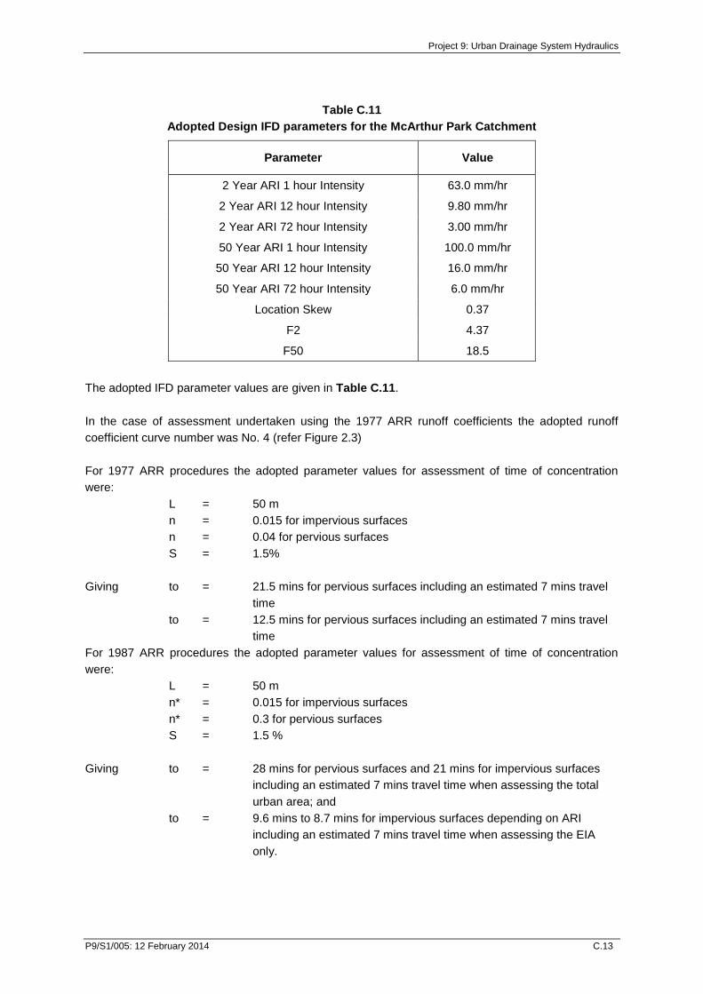
Project 9: Urban Drainage System Hydraulics
P9/S1/005: 12 February 2014 C.13
Table C.11
Adopted Design IFD parameters for the McArthur Park Catchment
Parameter Value
2 Year ARI 1 hour Intensity 63.0 mm/hr
2 Year ARI 12 hour Intensity 9.80 mm/hr
2 Year ARI 72 hour Intensity 3.00 mm/hr
50 Year ARI 1 hour Intensity 100.0 mm/hr
50 Year ARI 12 hour Intensity 16.0 mm/hr
50 Year ARI 72 hour Intensity 6.0 mm/hr
Location Skew 0.37
F2 4.37
F50 18.5
The adopted IFD parameter values are given in Table C.11.
In the case of assessment undertaken using the 1977 ARR runoff coefficients the adopted runoff
coefficient curve number was No. 4 (refer Figure 2.3)
For 1977 ARR procedures the adopted parameter values for assessment of time of concentration
were:
L = 50 m
n = 0.015 for impervious surfaces
n = 0.04 for pervious surfaces
S = 1.5%
Giving to = 21.5 mins for pervious surfaces including an estimated 7 mins travel
time
to = 12.5 mins for pervious surfaces including an estimated 7 mins travel
time
For 1987 ARR procedures the adopted parameter values for assessment of time of concentration
were:
L = 50 m
n* = 0.015 for impervious surfaces
n* = 0.3 for pervious surfaces
S = 1.5 %
Giving to = 28 mins for pervious surfaces and 21 mins for impervious surfaces
including an estimated 7 mins travel time when assessing the total
urban area; and
to = 9.6 mins to 8.7 mins for impervious surfaces depending on ARI
including an estimated 7 mins travel time when assessing the EIA
only.
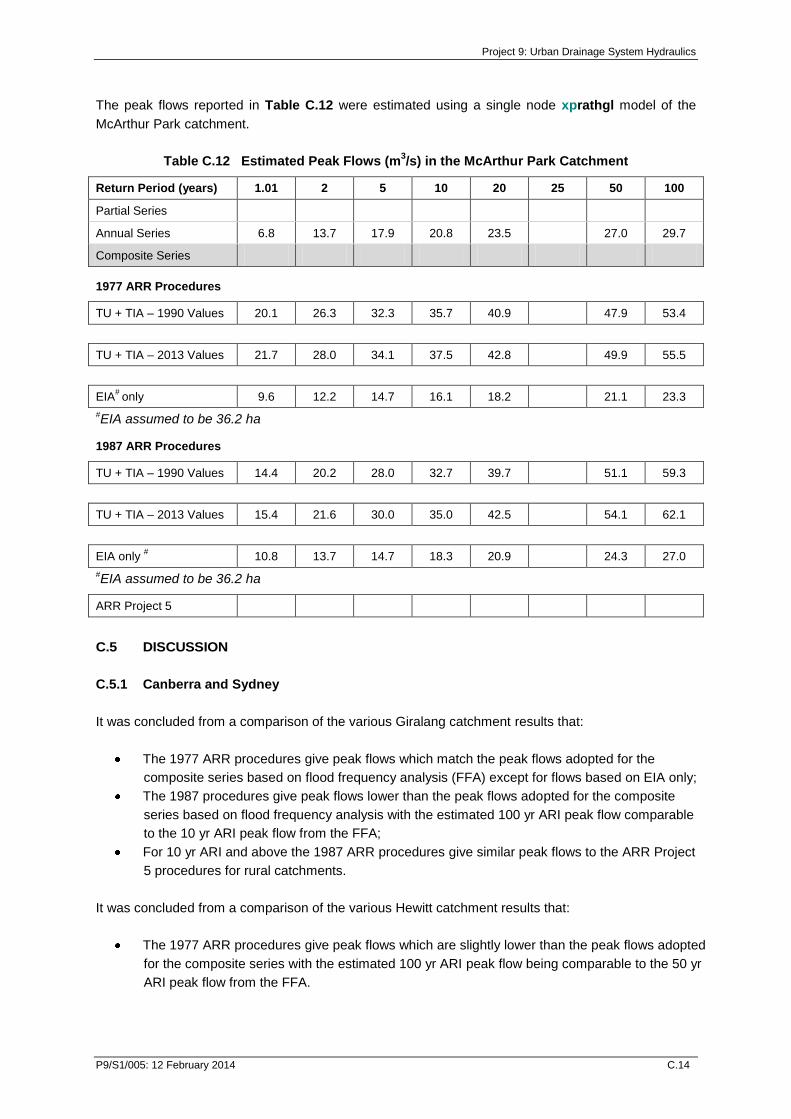
Project 9: Urban Drainage System Hydraulics
P9/S1/005: 12 February 2014 C.14
The peak flows reported in Table C.12 were estimated using a single node xprathgl model of the
McArthur Park catchment.
Table C.12 Estimated Peak Flows (m3/s) in the McArthur Park Catchment
Return Period (years) 1.01 2 5 10 20 25 50 100
Partial Series
Annual Series 6.8 13.7 17.9 20.8 23.5 27.0 29.7
Composite Series
1977 ARR Procedures
TU + TIA – 1990 Values 20.1 26.3 32.3 35.7 40.9 47.9 53.4
TU + TIA – 2013 Values 21.7 28.0 34.1 37.5 42.8 49.9 55.5
EIA#
only 9.6 12.2 14.7 16.1 18.2 21.1 23.3
#EIA assumed to be 36.2 ha
1987 ARR Procedures
TU + TIA – 1990 Values 14.4 20.2 28.0 32.7 39.7 51.1 59.3
TU + TIA – 2013 Values 15.4 21.6 30.0 35.0 42.5 54.1 62.1
EIA only # 10.8 13.7 14.7 18.3 20.9 24.3 27.0
#EIA assumed to be 36.2 ha
ARR Project 5
C.5 DISCUSSION
C.5.1 Canberra and Sydney
It was concluded from a comparison of the various Giralang catchment results that:
The 1977 ARR procedures give peak flows which match the peak flows adopted for the
composite series based on flood frequency analysis (FFA) except for flows based on EIA only;
The 1987 procedures give peak flows lower than the peak flows adopted for the composite
series based on flood frequency analysis with the estimated 100 yr ARI peak flow comparable
to the 10 yr ARI peak flow from the FFA;
For 10 yr ARI and above the 1987 ARR procedures give similar peak flows to the ARR Project
5 procedures for rural catchments.
It was concluded from a comparison of the various Hewitt catchment results that:
The 1977 ARR procedures give peak flows which are slightly lower than the peak flows adopted
for the composite series with the estimated 100 yr ARI peak flow being comparable to the 50 yr
ARI peak flow from the FFA.

Project 9: Urban Drainage System Hydraulics
P9/S1/005: 12 February 2014 C.15
The 1987 procedures give peak flows lower than the peak flows adopted for the composite
series with the estimated 100 yr ARI peak flow being comparable to the 10 yr ARI peak flow
from the FFA.
It was concluded from a comparison of the various Powells Creek catchment results that:
The 1977 ARR procedures give peak flows which are higher than the peak flows obtained from
an annual series analysis of gauged flows with the peak flows estimated for frequent runoff up
to 10 yr ARI being significantly higher;
One approach to improve agreement would be to test Curve No. 6 in comparison with the
adopted Curve No. 5;
The 1987 procedures give peak flows slightly higher than the peak flows adopted for the
annual series but in good agreement.
It was concluded in the 1989 Part I study in the ACT that the runoff coefficients and the time of
concentration are paired ie. any procedure to estimate each in a gauged urban catchments needs to
be undertaken simultaneously not independently as occurred when preparing the 1987 ARR. This
conclusion is further supported by these preliminary analyses.
C.5.2 Melbourne
Based on the results presented in Table C.8 it is apparent all Rational Method peak flows are
significantly higher than corresponding flood frequency peak flow estimates except where agreement
is forced by adjusting the runoff coefficient or the time of concentration.
Based on the work of Pomeroy et al (2013) the Kinkora Road urban catchment shares many
characteristics with the Powells Creek urban catchment in Sydney. The peak flows in both
catchments appear to derive mostly from the EIA only. This may well encompass only the roads
themselves plus very limited amounts of in block hard surfaces.
This also highlights the potential problems of adopting a limited number of long term gauged urban
catchments as representative of all urban catchments. The Kinkora Road and Powells Creek
catchments are probably representative of many older suburbs which were first developed in the
1950s or 1960s. They are however not representative of newer catchments with high degrees of
directly connected impervious areas including the Hewitt catchment in Sydney and the Giralang
catchment in ACT.
C.5.3 Darwin
It was concluded from a comparison of the various Moil results that:
The 1977 ARR procedures give peak flows which are slightly higher than the peak flows
adopted for the composite series (based on the adoption of Curve 6 for runoff coefficients);
The 1987 procedures give peak flows higher than the peak flows adopted for the composite
series for events greater than a 10 yr ARI event.
It was found that most predicted peak flows estimated using the 1977 ARR or 1987 ARR procedures
gave peak flows considerably higher than the peak flows estimated using FFA of the gauged flows
from the McArthur Park.

Project 9: Urban Drainage System Hydraulics
P9/S1/005: 12 February 2014 C.16
While one approach to improve agreement would be to test Curve No. 5 in comparison with the
adopted Curve No. 4 it was noted however that these FFA results are problematic due to the
presence of a large retarding basin located upstream of the gauging station which can modify
the runoff response from a significant proportion of the catchment by infiltrating any overland
flows into the grassed base of the basin in frequent events and by reducing peak flows in major
events.

APPENDIX D
PRELIMINARY PART II STUDY – CANBERRA & SYDNEY

Project 9: Urban Drainage System Hydraulics
P9/S1/005: 12 February 2014 D.1
D.1 BACKGROUND
In 1993 a study was undertaken in Canberra to provide practice guidelines when utilising hydrograph
based estimation procedures in urban drainage projects in the ACT. The work followed on from the
earlier Part I study. It is described in a report titled “Drainage Design Practice Part II”, Willing and
Partners (1993) which is attached in Appendix F.
The goal of the Part II study was to test several currently available rainfall/runoff computer programs
including RAFTS, RORB and IlSAX on Canberra's gauged urban catchments.
In particular, the objectives were to determine appropriate:
(iv) design rainfall loss rate estimation parameters applicable to individual programs,
(v) surface runoff routing parameters for pervious and impervious areas specific to each program
tested, and
(vi) design storm event modelling procedures specific to each program tested.
The assessment of RAFTS model parameters was summarised as follows (Willing & Partners, 1993):
The RAFTS analysis in this study involved the use of two approaches to rainfall loss estimation. They
were the initial/continuing loss approach and the infiltration/water balance procedure approach which
utilizes the Australian Representative Basin Program (ARBM).
The Giralang catchment analysis results were based on a 41 node RAFTS-XP network which is
equivalent to an average sub-catchment size of approximately 2.2 hectares. The Mawson catchment
analysis results were based on a 180 node network which is equivalent to an average sub-catchment
size of approximately 2,3 hectares.
The initial/continuing loss model analysis failed to produce a single set of loss rates which were able
to model the full range of flood frequency curve flows on the catchments modelled. The results
indicated the peak flows are sensitive to the losses adopted.
Analysis was carried out on the Giralang and Mawson catchments to determine the effect of the level
of sub-catchment discretisation adopted. The conclusion to be drawn from this analysis was that the
modelled peak flow increases with increasing catchment discretisation. Alternatively the modelled
peak flows decrease with decreasing catchment discretisation.
The RAFTS ARBM loss model approach to calibration was to vary the initial catchment wetness
conditions until a volume calibration was achieved against the targeted flood hydrograph.
Following this a further calibration against the targeted peak flow was carried out by varying the
catchment surface roughness parameters.
The results of the RAFTS ARBM modelling produced a high level of calibration achievement particular
on the Giralang catchment which is well gauged. The design storm event modelling against the
catchment flood frequency curves also revealed that single set of model parameter values was able to
reasonably predict a full range of the ARI flood frequency flows. The results of the design storm
analysis should be viewed with some caution due to the uncertainty which exists regarding the
catchment flood frequency curves, particularly at the higher magnitude ARI events.

Project 9: Urban Drainage System Hydraulics
P9/S1/005: 12 February 2014 D.2
The ACT Department of Urban Services publication titled “Design Standards for Urban Infrastructure,
1 Stormwater” subsequently specified recommended parameters and procedures for hydrograph
estimation to be used instead of values and procedures recommended in program documentation and
related reports. The guidance was as follows.
Rainfall Loss Rates
The XP-RAFTS program offers a choice between two approaches to rainfall loss estimation.
They are the initial/continuing loss model and the infiltration/water balance procedure which
utilises the Australian Representative Basins Model (ARBM). The use of the ARBM loss model
shall be used in preference to the initial/continuing loss model due to the ability of ARBM to
model a range of ARI events with a single set of model parameters.
The values for the ARBM loss model to be adopted are as follows.
Parameter
Adopted
Value
Initial
Value
Storage Capacities
Impervious (IMP) 0.50 0.0
Interception (ISC) 1.00 0.0
Depression (DSC) 1.00 0.0
Upper soil (USC) 25.00 20.00
Lower soil (LSC) 50.00 40.00
Infiltration
Dry soil sorptivity (SO) 3.00
Hydraulic conductivity (K0) 0.33
Lower soil drainage factor (LDF) 0.05
Groundwater recession;
constant rate (KG) 0.94
variable rate (GN) 1.00
Evapo-Transpiration
Proportion of rainfall intercepted by vegetation (IAR) 0.70
Max potential evapo-transpiration;
upper soil (UH) 10.00
lower soil (LH) 10.00
Proportion of evapo-transpiration from upper soil zone (ER) 0.70
Ratio of potential evaporation to A class pan (ECOR) 0.90
Surface Runoff Routing
The following surface runoff routing parameters shall be adopted.
Parameter Value
Impervious surface roughness 0.015
Pervious surface roughness 0.040
Non-linearity coefficient (default) 0.285

Project 9: Urban Drainage System Hydraulics
P9/S1/005: 12 February 2014 D.3
Rainfall Gauge
Flow Gauge
Rural Area
Outlet Paired micro catchments
Isochronal Contours
160
140
120
100
80
60
40
20
180
120
140
160
140
60
40
Since the 1993 study was completed an addition of 20+ years of rainfall and runoff data collected
including 3 years of data collected on micro catchments embedded within the Giralang urban
catchment. Data from the micro catchments was collected and reported in the PhD thesis submitted
by Goyen in 2000. The research reported by Goyen, 2000 further examined the processes within the
Giralang catchment as well as the Hewitt urban catchment located near Penrith in Sydney.
A potential problem with Part II study was the recommended initial (and high) values for moisture
stores. An embedded approach has been assessed to establish if it performs better than fixed initial
values in a vertical water balance loss model.
D.2 GIRALANG
The details of the Giralang urban catchment and its gauging stations are provided by Goyen (2000).
An overview of the Giralang catchment is given in Figure D.1 while details on the paired micro
catchments are given in Figures D.2 and D.3.
As part of the preparation of this position paper both the ACT Part II study carried out in 1993 as well
as the research carried out by Goyen (2000) was revisited.
Figure D.1 Giralang Gauged Urban Catchment
ACTEW Flow
Gauging Station
No. 410763
ACTEW
Rainfall Station
No. 570987
ACTEW
Rainfall Station
No. 570991
ACTEW
Rainfall Station
No. 570992
(2.47 ha)
(19.6 ha)
Fully Urban Area
(62.9 ha)

Project 9: Urban Drainage System Hydraulics
P9/S1/005: 12 February 2014 D.4
Figure D.2 Giralang Gauged Urban Micro Catchments (after Goyen, 2000)
Figure D.3 Giralang Gauged Urban Micro Catchment Gauges (after Goyen, 2000)
Paling fences run along rear
boundaries to prevent most yard
water entering lower allotments Rainfall Gauge
12 Lot roofs only
Micro catchment No. 1
14 Lot roofs, yards and
roadway
Micro catchment No. 2
12 Lot Flow Gauge located
on 300mm pipe outlet
14 Lot Flow Gauge located
on 450mm pipe outlet
Rainfall Gauge

Project 9: Urban Drainage System Hydraulics
P9/S1/005: 12 February 2014 D.5
Figure D.4 Conceptual Representation of Isochronal Modelling Approach
applied to xprafts
The methods described by Goyen, 2000 have been incorporated into the sub-catchment hydrograph
estimation module of xprafts. The modifications to the xprafts analysis procedure included an
alternate sub-catchment analysis procedure that is indicated diagrammatically in Figure D.4.
Runoff is estimated separately for the roof and gutter, adjacent road surface and paving and pervious
gardens and lawn areas. A virtual allotment drainage network is constructed to represent lagging,
bypass, capture and additional storage routing and infiltration/ evapotranspiration within the various
WSUD facilities. The outputs from each structure as well as any bypass flows are combined to give
the total runoff hydrograph from a typical allotment.
The method allows the definition of a wide range of WSUD/LID facilities including allotment storage
devices, infiltration beds and rain water tanks. The procedures allows for variable structure sizes as
well as variable capture and bypass percentages. Additional parameters to define the percentage
breakdown in impervious surfaces between roofs, paving and road surfaces was also included.
The models as described by Goyen (2000) were adopted without any modification apart from the
addition of evaporation from impervious surfaces during the extended duration summer daytime
events.
The RAFTS model developed as part of the research, which analysed gauging data collected in the
micro catchments in the period 1993-1995, has been used in this analysis together with the updated
total catchment flow gauging up to 2013.
A review of the original calibration was carried out using four separate storm events from the 1993 –
1995 dataset. These included events on the 3 January 1993, 6 March 1993, 5 April 1993 and 13 May
1995 that represented a range of events between <1 yr ARI to around 8 yr ARI.
Allotments
in Isochronal
Slice
6
13
20
27
39
33
26
19
18
5
Sub-Catchment Outlet
Single Allotment with
WSUD/LID Facilities

Project 9: Urban Drainage System Hydraulics
P9/S1/005: 12 February 2014 D.6
This allowed a review of events that were predominately impervious area runoff only through to
events that only had pervious area runoff in the later portions of the event to an event that had a
significant proportion of pervious area runoff. Figures D.5 – D.8 show the fit between the simulated
flows and the gauged flows for both the 1.27ha embedded Micro catchment No. 1 (14 Lots), and the
62.9 ha urban catchment (526 Lots).
(a) Micro Catchment No. 1 (R2 = 0.924)
(b) Giralang Urban Catchment ((R2 = 0.894)
Figure D.5 Observed and Predicted Flows during Storm of 13 May 1995

Project 9: Urban Drainage System Hydraulics
P9/S1/005: 12 February 2014 D.7
Micro Catchment No. 1 (R2 = 0.992)
Figure D.6 Observed and Predicted Flows during Storm of 5 April 1993
Micro Catchment No. 1 ((R2 = 0.977)
Figure D.7 Observed and Predicted Flows during Storm of 6 March 1993

Project 9: Urban Drainage System Hydraulics
P9/S1/005: 12 February 2014 D.8
(a) Micro Catchment No. 1 (R2 = 0.945)
(b) Giralang Urban Catchment ((R2 = 0900)
Figure D.8 Observed and Predicted Flows during Storm of 3 January 1993

Project 9: Urban Drainage System Hydraulics
P9/S1/005: 12 February 2014 D.9
The above review and the 2000 analysis used only the micro catchment rainfall gauge that is located
near the centre of the overall catchment.
The coefficient of determination (R2) for Micro catchment No. 1 for all events was in excess of 0.92
with minimal rainfall variation across the micro catchment. The coefficient of determination R2 for the
urban catchment for both events reviewed were greater than 0.9. The differences in level of
agreement between observed and predicted flows from Micro catchment No. 1 and the urban
catchment were mainly attributed to spatial variations in rainfall across the overall catchment.
Goyen, 200 reported that the area ratio between Micro catchment No. 1 and the urban catchment was
49.5 the ratio of the peak flows observed peak flows varied between 27.9 and 49.4. Of the 8 larger
events in excess of a 1 yr ARI event the average ratio was 35.3 while the average ratio for the 24
smaller events was 37.0. The variation was attributed to spatial variance both in rainfall depths as
well as variance in the temporal distribution of rainfall.
Based on the 1993 – 1995 gauging period the above variations suggest that when rainfall variation is
not explicitly taken into account the errors in estimated peak flows could be up to +/-30%. This spatial
variation over small urban catchments was much larger than reported in the literature. While
Project 2 Spatial Patterns of Design Rainfall provides guidance on areal reduction factors the
minimum catchment area is 100 ha and the minimum storm duration is 1 hour. In the case of the ACT
the latest guidance would give a 3.3% reduction of the point rainfall intensity.
Despite the above reservations in respect to rainfall variance over even small urban catchments the
above the calibration review above demonstrates that it is possible to calibrate urban catchments to
historical events to an acceptable level of accuracy. This has been made possible mainly via the
replacement of simple initial loss/continuing loss rate model with a more physically based water
balance model with separate testing of infiltration and saturation/drainage at each modelling time
step.
This review was of complete storms and could have just as easily been applied to complete
continuous rainfall records as has been undertaken in other studies.
In the past it has been difficult to transfer calibrated urban catchment models into a design mode to
estimate flow quantiles usually between 1 yr ARI and 100 yr ARI.
The current practice when using rainfall-runoff models to estimate flow quantiles in ungauged
catchments is the apply a dimensionless design rainfall burst temporal pattern to the rainfall intensity
return period of interest determined in accordance with ARR procedures..
The main issues in this regard have been the lack of recommendations for appropriate rainfall losses
to apply when assessing each of the flow quantiles. Additionally, while the rainfall losses which have
been applied are intended to represent infiltration they also tend to try and compensate for areal
rainfall variance and for any difficulties in the calibration. In the case of the 1993 Part II study it was
found that in order to match the flow quantiles obtained from FFA that the initial pervious rainfall loss
needed to increase with increasing ARI ie. the 2 yr ARI peak flow was best fitted by a 5.0 mm initial
pervious area rainfall loss while the 100 yr ARI peak flow was best fitted by a 15.0 mm initial pervious
area rainfall loss.

Project 9: Urban Drainage System Hydraulics
P9/S1/005: 12 February 2014 D.10
Since the 1993 Part II study in the ACT further development has occurred within the RAFTS
modelling system as described by Goyen (2000). In particular development of the ARBM based
rainfall loss and water balance model was altered to allow a distribution of porosity across the
pervious surfaces to better reflect the variation experienced across urban allotments. This behaviour
was previously postulated as far back as 1965 by Lindsay and Crawford in their development of the
Stanford Watershed Model.
In the 1993 Part II study the ARBM did not contain the distribution capability and as such only a single
set of values were provided (refer Appendix D.1). The distribution of porosity has allowed a more
realistic calibration tool that now better simulates the commencement of pervious runoff by varying
infiltration rates across pervious areas.
The design storm concept in this discussion paper was further tested using the calibrated Giralang
catchment (enhanced) RAFTS model and embedding the ARR design storm burst temporal patterns
in the storm recorded on 3 January 1993. The 25 minute ARR design burst pattern was embedded
first at the commencement of the event and then separately at the commencement of the first major
peak some 1 hour and 15 minutes into the event.
The results from this analysis of the Giralang urban catchment (62.9 ha) are summarised in
Table D.1.
Table D.1 Estimated Peak Flows for Embedded Storm of 3 January 1993
on Giralang Catchment
ARI Rainfall Rainfall 5 minute Temporal Partition Peak Flow
(yrs) Intensity
(mm/h)
Depth
(mm)
No. 1
(mm)
No. 2
(mm)
No. 3
(mm)
No. 4
(mm)
No. 5
(mm)
FFA
(m3/s)
Early*
(m3/s)
Middle**
(m3/s)
1 27.1 11.3 1.92 3.16 4.41 1.02 0.79 4.3 3.10 4.15
2 35.5 14.8 2.51 4.14 5.77 1.33 1.04 6.7 4.38 5.56
5 46.9 19.5 3.32 5.47 7.62 1.76 1.37 8.2 6,78 8.12
10 54.2 22.6 3.84 6.33 8.81 2.03 1.58 9.2 7.55 9.44
20 64.0 26.6 4.53 7.46 10.39 2.40 1.87 11.3 10.06 12.11
50 77.4 32.3 5.81 8.39 11.29 3.55 3.22 12.7 12.51 13.82
100 88.3 36.8 6.62 9.56 12.87 4.04 3.68 14.2 16.05 17.16
* “Early” refers to embedment of the ARR storm burst at the start of the storm
**“Middle” refers to the embedment of the ARR storm burst at the commencement of the first major
peak some 1 hour and 15 minutes into the event
It was also found that when the design storm was embedded under the second major historical peak
around 3 hours and 15 minutes after the commencement of the storm the resulting 10 yr ARI peak
flow was found to be 9.40 m3/s or slightly less than the embedment under the first major peak. This
was due to the intervening dry period that allowed the re-establishment of the infiltration capacity and
the degree of saturation of the soil upper store.
It was concluded that “middle” embedment gave peak flows which were the best overall fit to the peak
flows calculated by FFA.

Project 9: Urban Drainage System Hydraulics
P9/S1/005: 12 February 2014 D.11
While it was expected that the estimated peak flows would be higher than the FFA estimates due to
the use of point IFD data it was found that the estimated peak flows for events up to the 5 yr ARI were
slightly lower than the FFA estimates while the estimated peak flows for events greater than or equal
to 10 yr ARI were slightly higher than the FFA estimates. The steeper slope of the estimated flood
frequency curve may be due to the design storm burst temporal pattern. It may also be due to the
expectation that analysing the storm burst of a given ARI yields a peak runoff of the same ARI which
may not be correct on average.
The only way that estimated peaks could better match the peak flows estimated by FFA would be to
abandon the design storm approach and instead directly model the annual maximum runoff events as
well as additional events to create partial series data ie. to create a synthetic database of peak flows
which could be analysed using FFA.
If the simulation of historical storms is able to match the observed events as closely as achieved in
the Giralang catchment in the period 1993 – 1995 then the resulting flow quantiles obtained from FFA
of the simulated peak flows should closely match the flow quantiles derived from the gauged peak
flows.
D.2 HEWITT
The details of the Hewitt urban catchment and its gauging stations are provided by Goyen (2000). An
overview of the Hewitt catchment is given in Figure D.9.
Figure D.9 Hewitt Urban Catchment (after Figure 4.1, Wilkinson (1995))
Raingauges
Flowgauge

Project 9: Urban Drainage System Hydraulics
P9/S1/005: 12 February 2014 D.12
Hewitt Urban Catchment ((R2 = 0.903)
Figure D.11 Observed and Predicted Flows during Storm of 15 February 1994
The original calibration was carried out using three separate storm events including the storm of
15 February 1994. Figure D.11 shows the fit between the simulated flows and the gauged flows for
the 62 ha urban catchment (556 Lots).
The design storm concept in this discussion paper was further tested using the calibrated Hewitt
catchment (enhanced) RAFTS model and embedding the ARR design storm burst temporal patterns
in the storm recorded on 15 February 1994. The results from this analysis of the Hewitt urban
catchment (62 ha) are summarised in Table D.2.
Table D.2 Estimated Peak Flows for Embedded Storm of 3 January 1993
on Hewitt Catchment
ARI Rainfall Rainfall 5 minute Temporal Partition Peak Flow
(yrs) Intensity
(mm/h)
Depth
(mm)
No. 1
(mm)
No. 2
(mm)
No. 3
(mm)
No. 4
(mm)
No. 5
(mm)
FFA
(m3/s)
Early*
(m3/s)
Middle**
(m3/s)
1 37.2 15.5 2.64 4.34 6.05 1.40 1.08 3.85 4.49
2 48.1 20.0 3.41 5.61 7.82 1.80 1.40 5.00 6.22
5 62.4 26.0 4.42 7.29 10.15 2.34 1.82 7.57 10.07
10 70.9 29.5 5.02 8.27 11.52 2.66 2.07 8.95 11.76
20 82.0 34.2 5.81 9.56 13.32 3.07 2.39 13.38 15.80
50 96.6 40.2 7.24 10.46 14.08 4.43 4.02 16.22 18.32
100 107.8 44.9 8.08 11.67 15.72 4.94 4.49 20.96 22.80

Project 9: Urban Drainage System Hydraulics
P9/S1/005: 12 February 2014 D.13
It should be noted that the depth of rainfall in the Hewitt catchment is between 22% and 37% higher
than Giralang. This not only increases flow peaks due to increased rainfall intensity it also potentially
saturates the upper soil stores within pervious areas during an event. This could have the effect of
increasing flow peaks if the primary storm burst is embedded later in the event.

APPENDIX E
WILLING AND PARTNERS (1989) DRAINAGE DESIGN PRACTICE FOR LAND DEVELOPMENT IN THE ACT.
PART I: RATIONAL FORMULA PROCEDURES


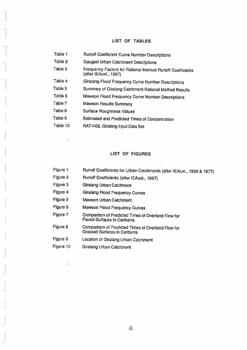
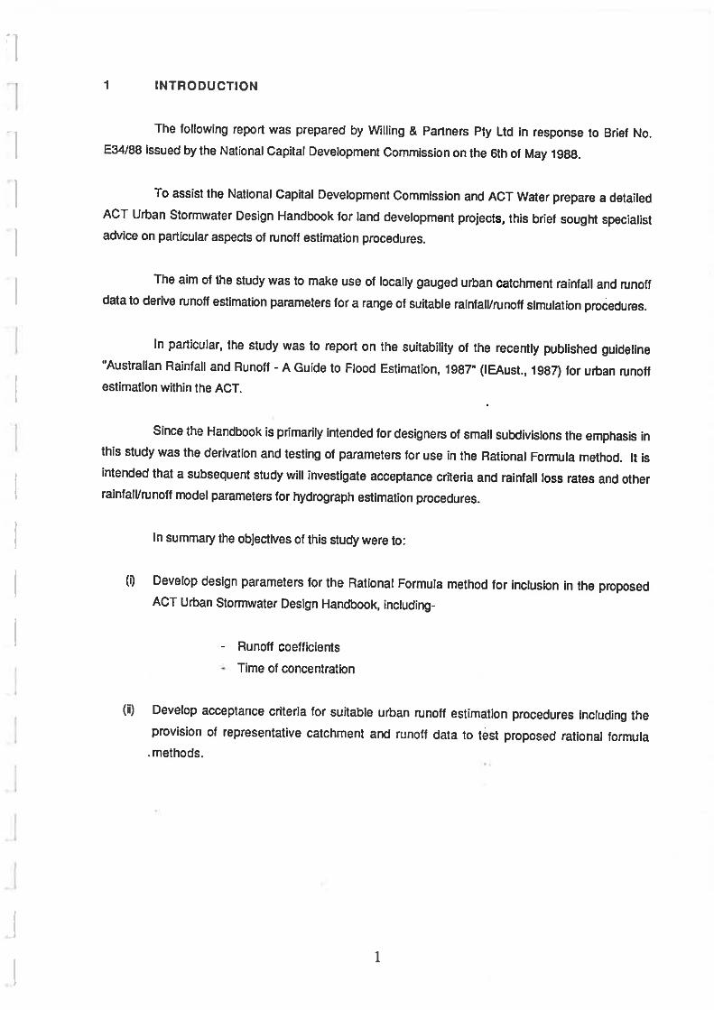


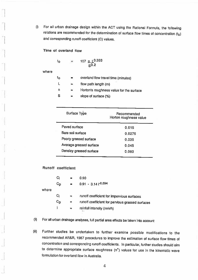


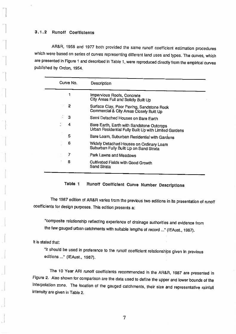


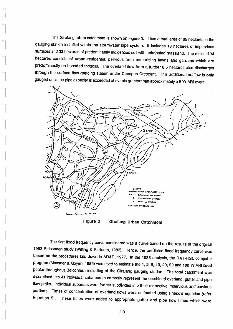


APPENDIX F
WILLING AND PARTNERS (1993) DRAINAGE DESIGN PRACTICE PART II