aus hamburg gottingen, 2006¨
TRANSCRIPT
Quantendynamik von SN2–Reaktionen
Dissertation
zur Erlangung des Doktorgradesder Mathematisch–Naturwissenschaftlichen Fakultaten
der Georg–August–Universitat zu Gottingen
vorgelegt von
Carsten Hennig
aus Hamburg
Gottingen, 2006
D7
Referent: Priv.–Doz. Dr. Stefan Schmatz
Korreferent: Prof. Dr. Michael Buback
Tag der mundlichen Prufung: 01.11.2006
Quantum Dynamics of SN2 Reactions
Dissertation
submitted to theCombined Faculties for the Natural Sciences
and for Mathematicsof the Georg–August–Universitat of Gottingen
for the degree ofDoctor of Natural Sciences
presented by
Carsten Hennig
born in Hamburg
Gottingen, 2006
Referees: Priv.–Doz. Dr. Stefan SchmatzProf. Dr. Michael Buback

Kurzfassung
In dieser Arbeit werden einige quantenmechanische Untersuchungen des Reak-tionsmechanismus in nukleophilen bimolekularen Substitutionsreaktionen (SN2–Reak-tionen) vorgestellt. Der SN2–Mechanismus ist sowohl fur zahlreiche Gebiete der ex-perimentellen Chemie als auch fur die theoretischen Konzepte der Reaktionsdynamikvon Bedeutung. Entlang der Reaktionskoordinate befinden sich in der Gasphase zweitiefe Potentialtopfe, und Bindungsbruch und –bildung finden gleichzeitig statt. Da-durch weist die Reaktion einige interessante Besonderheiten wie Resonanzen ver-schiedenen Typs und die Moglichkeit zur Ruckkehr uber die Barriere auf. Mittelszeitunabhangiger quantenmechanischer Streurechnungen wird der Einfluss der sym-metrischen Schwingungen der Methylgruppe sowie von Rotationen des angegriffenenMethylhalogenids an zwei Beispielreaktionen in der Gasphase untersucht. Im erstenFall kann eine aktive Teilnahme der Moden an der Reaktion festgestellt und somitdas Konzept der Beobachtermoden dafur in Frage gestellt werden. Der zweite Fallzeigt die Bedeutung der Kopplung der Rotationsbewegung mit den reaktiven Freiheits-graden.
Abstract
This thesis presents quantum mechanical investigations of the mechanism involvedin nucleophilic bimolecular substitution reactions (SN2 reactions). The SN2 mech-anism is important both for applications in a wide field of chemistry as well as forthe theoretical concepts in reaction dynamics. In the gas phase, the presence of twodeep wells in the reaction profile before and after passage of the central barrier andthe simultaneous breaking and forming of bonds give rise to several interesting fea-tures like resonances of different types and the possibility of recrossing the barrier.Time–independent quantum mechanical scattering theory is applied to investigate therole of the symmetric vibrations of the methyl group and of rotations of the attackedmethyl halide for two model reactions in the gas phase. While the former can be shownto actively participate in the reaction, questioning the spectator mode concept in thiscase, the investigation of the latter reveals the importance of the coupling of rotationalmotion with the reactive degrees of freedom.
Contents
1 Introduction 1
2 Theoretical Framework 52.1 Coordinate Systems and Hamiltonians . . . . . . . . . . . . . . . . . 5
2.1.1 Jacobi Coordinates . . . . . . . . . . . . . . . . . . . . . . . 52.1.2 Hyperspherical Coordinates . . . . . . . . . . . . . . . . . . 8
2.2 Scattering Formalism . . . . . . . . . . . . . . . . . . . . . . . . . . 82.3 Strategies for the Treatment of Rotation . . . . . . . . . . . . . . . . 9
3 Numerical Methods 113.1 R–Matrix Propagation . . . . . . . . . . . . . . . . . . . . . . . . . 113.2 Collocation Method: Basic Properties . . . . . . . . . . . . . . . . . 12
3.2.1 A Simple Example . . . . . . . . . . . . . . . . . . . . . . . 123.2.2 Spectral Accuracy . . . . . . . . . . . . . . . . . . . . . . . 143.2.3 Generating a Matrix Representation . . . . . . . . . . . . . . 15
3.3 Collocation Method and Orthogonal Polynomials . . . . . . . . . . . 173.3.1 Orthogonal Polynomials . . . . . . . . . . . . . . . . . . . . 173.3.2 Collocation Basis . . . . . . . . . . . . . . . . . . . . . . . . 21
3.4 Generalizations . . . . . . . . . . . . . . . . . . . . . . . . . . . . . 283.4.1 Several Dimensions . . . . . . . . . . . . . . . . . . . . . . . 283.4.2 Arbitrary Orthogonal Functions . . . . . . . . . . . . . . . . 303.4.3 Comparison to Finite Elements . . . . . . . . . . . . . . . . . 33
3.5 PODVR of the Schroedinger Equation . . . . . . . . . . . . . . . . . 343.6 Diagonalization Techniques . . . . . . . . . . . . . . . . . . . . . . . 35
3.6.1 Error Measure . . . . . . . . . . . . . . . . . . . . . . . . . 363.6.2 Lanczos with Partial Reorthogonalization . . . . . . . . . . . 363.6.3 The Jacobi–Davidson Method . . . . . . . . . . . . . . . . . 383.6.4 Combining Lanczos and Jacobi–Davidson . . . . . . . . . . . 39
4 Results 414.1 Cl–Cl Exchange Reaction . . . . . . . . . . . . . . . . . . . . . . . . 41
4.1.1 Abstract . . . . . . . . . . . . . . . . . . . . . . . . . . . . . 414.1.2 Introduction . . . . . . . . . . . . . . . . . . . . . . . . . . . 42

CONTENTS ii
4.1.3 Results . . . . . . . . . . . . . . . . . . . . . . . . . . . . . 434.1.4 Conclusions . . . . . . . . . . . . . . . . . . . . . . . . . . . 61
4.2 Cl–Br Exchange Reaction . . . . . . . . . . . . . . . . . . . . . . . . 624.2.1 Abstract . . . . . . . . . . . . . . . . . . . . . . . . . . . . . 624.2.2 Introduction . . . . . . . . . . . . . . . . . . . . . . . . . . . 634.2.3 Results . . . . . . . . . . . . . . . . . . . . . . . . . . . . . 644.2.4 Conclusions . . . . . . . . . . . . . . . . . . . . . . . . . . . 80
4.3 Rate Constants in the Cl–Cl Exchange Reaction . . . . . . . . . . . . 814.3.1 Abstract . . . . . . . . . . . . . . . . . . . . . . . . . . . . . 814.3.2 Introduction . . . . . . . . . . . . . . . . . . . . . . . . . . . 824.3.3 Results . . . . . . . . . . . . . . . . . . . . . . . . . . . . . 834.3.4 Conclusions . . . . . . . . . . . . . . . . . . . . . . . . . . . 93
4.4 Rotational Effects in the Cl–Br Reaction . . . . . . . . . . . . . . . . 944.4.1 Potential Energy Surface . . . . . . . . . . . . . . . . . . . . 944.4.2 Numerical Details . . . . . . . . . . . . . . . . . . . . . . . 974.4.3 Results . . . . . . . . . . . . . . . . . . . . . . . . . . . . . 98
5 Summary and Outlook 103
Bibliography 107
Chapter 1
Introduction
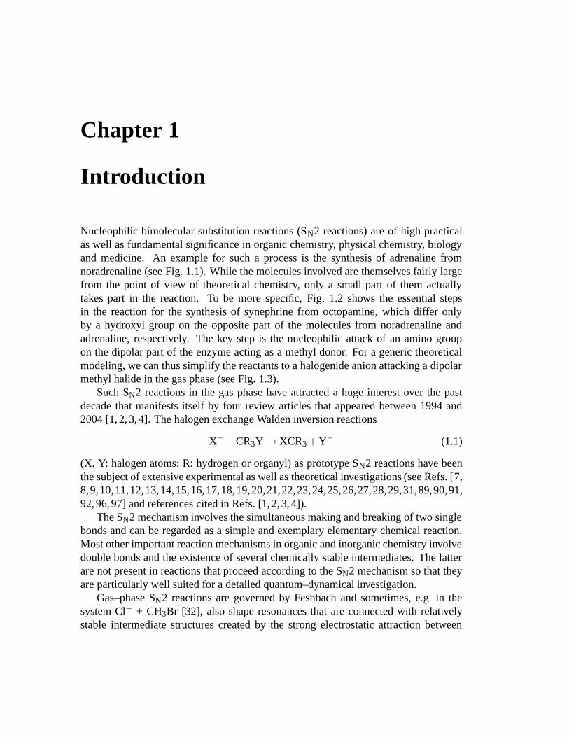
Nucleophilic bimolecular substitution reactions (SN2 reactions) are of high practicalas well as fundamental significance in organic chemistry, physical chemistry, biologyand medicine. An example for such a process is the synthesis of adrenaline fromnoradrenaline (see Fig. 1.1). While the molecules involved are themselves fairly largefrom the point of view of theoretical chemistry, only a small part of them actuallytakes part in the reaction. To be more specific, Fig. 1.2 shows the essential stepsin the reaction for the synthesis of synephrine from octopamine, which differ onlyby a hydroxyl group on the opposite part of the molecules from noradrenaline andadrenaline, respectively. The key step is the nucleophilic attack of an amino groupon the dipolar part of the enzyme acting as a methyl donor. For a generic theoreticalmodeling, we can thus simplify the reactants to a halogenide anion attacking a dipolarmethyl halide in the gas phase (see Fig. 1.3).
Such SN2 reactions in the gas phase have attracted a huge interest over the pastdecade that manifests itself by four review articles that appeared between 1994 and2004 [1, 2, 3, 4]. The halogen exchange Walden inversion reactions
X− +CR3Y → XCR3 +Y− (1.1)
(X, Y: halogen atoms; R: hydrogen or organyl) as prototype SN2 reactions have beenthe subject of extensive experimental as well as theoretical investigations (see Refs. [7,8,9,10,11,12,13,14,15,16,17,18,19,20,21,22,23,24,25,26,27,28,29,31,89,90,91,92, 96, 97] and references cited in Refs. [1, 2, 3, 4]).
The SN2 mechanism involves the simultaneous making and breaking of two singlebonds and can be regarded as a simple and exemplary elementary chemical reaction.Most other important reaction mechanisms in organic and inorganic chemistry involvedouble bonds and the existence of several chemically stable intermediates. The latterare not present in reactions that proceed according to the SN2 mechanism so that theyare particularly well suited for a detailed quantum–dynamical investigation.
Gas–phase SN2 reactions are governed by Feshbach and sometimes, e.g. in thesystem Cl− + CH3Br [32], also shape resonances that are connected with relativelystable intermediate structures created by the strong electrostatic attraction between

CHAPTER 1. INTRODUCTION 2
Figure 1.1: Synthesis of adrenaline from noradrenaline by addition of a methyl groupwhich proceeds via an SN2 mechanism [5].
Figure 1.2: Detailed steps in the synthesis of synephrine from octopamine [6].

3
Figure 1.3: Potential along the reaction coordinate for the Cl–Br exchange reactionCl−+CH3Br→Br−+CH3Cl (see [102]).
the attacking nucleophile, mostly an ion, and the dipolar substrate molecule, often amethyl halide. As is well known [1, 2, 3, 4, 7, 8, 9], two relatively deep wells (ca. 0.5eV) are present in the reaction profile that correspond to two complexes X− · · · CH3Yand XCH3 · · · Y− being formed before and after passage of the central barrier.
It was shown by Hase and co–workers in a series of papers on classical dynamicscalculations on these reactions [20, 21, 22, 25, 26, 27, 28, 30, 97] that there is only avery limited energy flow between the inter– and intramolecular modes of the collisioncomplex so that a detailed quantum–dynamical study is required. In particular, it isworth investigating whether excitation of particular vibrational and/or rotational modesin the reactant molecule result in a non–negligible influence on the reactivity in gas–phase SN2 reactions. Moreover, state–selected reaction probabilities and cross sectionsgive valuable information on vibrational and/or rotational product distributions.
This thesis presents quantum mechanical studies on two model systems, the sym-metric chlorine–chlorine exchange reaction
Cl− + CH3Cl′ → ClCH3 + Cl′−
and the exothermic bromine–chlorine substitution
Cl− + CH3Br → ClCH3 + Br−.
Using time–independent quantum mechanical scattering theory, the symmetric vibra-tions of the methyl group (umbrella bend and C–H stretch) are treated exactly within

CHAPTER 1. INTRODUCTION 4
C3v symmetry for the first time, shedding more light on the active role of the methylgroup in the Walden inversion. In addition, methods and results on the inclusion ofthe rotational motion of the methyl halide are shown, providing the first state–selectivetreatment of spatial degrees of freedom beyond collinearity in heavy six–atom reac-tions with long–range interaction potentials. For that purpose, numerical techniquesare presented in detail and suitable extensions are proposed.
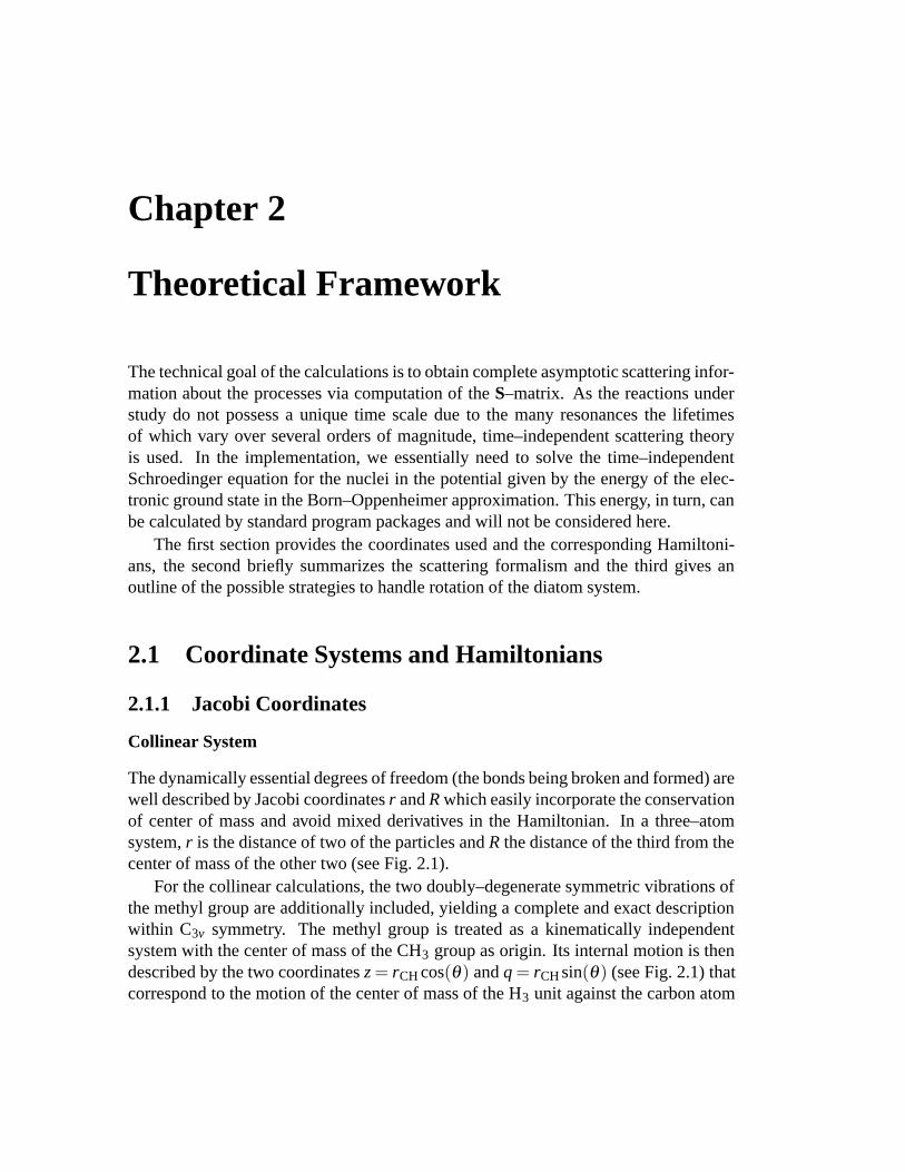
Chapter 2
Theoretical Framework
The technical goal of the calculations is to obtain complete asymptotic scattering infor-mation about the processes via computation of the S–matrix. As the reactions understudy do not possess a unique time scale due to the many resonances the lifetimesof which vary over several orders of magnitude, time–independent scattering theoryis used. In the implementation, we essentially need to solve the time–independentSchroedinger equation for the nuclei in the potential given by the energy of the elec-tronic ground state in the Born–Oppenheimer approximation. This energy, in turn, canbe calculated by standard program packages and will not be considered here.
The first section provides the coordinates used and the corresponding Hamiltoni-ans, the second briefly summarizes the scattering formalism and the third gives anoutline of the possible strategies to handle rotation of the diatom system.
2.1 Coordinate Systems and Hamiltonians
2.1.1 Jacobi Coordinates
Collinear System
The dynamically essential degrees of freedom (the bonds being broken and formed) arewell described by Jacobi coordinates r and R which easily incorporate the conservationof center of mass and avoid mixed derivatives in the Hamiltonian. In a three–atomsystem, r is the distance of two of the particles and R the distance of the third from thecenter of mass of the other two (see Fig. 2.1).
For the collinear calculations, the two doubly–degenerate symmetric vibrations ofthe methyl group are additionally included, yielding a complete and exact descriptionwithin C3v symmetry. The methyl group is treated as a kinematically independentsystem with the center of mass of the CH3 group as origin. Its internal motion is thendescribed by the two coordinates z = rCH cos(θ) and q = rCH sin(θ) (see Fig. 2.1) thatcorrespond to the motion of the center of mass of the H3 unit against the carbon atom

CHAPTER 2. THEORETICAL FRAMEWORK 6
Figure 2.1: Definition of the coordinate system for the four–dimensional collinearcalculations.
(z) and the ’breathing’ motion of the D3h–symmetric H3 unit in a plane perpendicularto the molecular axis of symmetry (q).
In these coordinates, the kinetic energy is completely decoupled and the Hamilto-nian reads
H = − h2
2μ1
∂ 2
∂R2 −h2
2μ2
∂ 2
∂ r2 −h2
2μ3
∂ 2
∂ z2 −h2
2μ4
∂ 2
∂q2 +V (R,r,z,q), (2.1)
where the reduced masses are given by
μ1 =mXmCH3Y
mX +mCH3Y, (2.2)
μ2 =mCH3mY
mCH3 +mY, (2.3)
μ3 =3mHmC
3mH +mC, (2.4)
andμ4 = 3mH. (2.5)
Here, mX and mY denote the masses of the two halogen atoms (i.e. the isotopes 35Cl or79Br) and mC and mH refer to the masses of the carbon and hydrogen atoms. V (R,r,z,q)is the energy of the electronic ground state with the nuclei at the positions specified by(R,r,z,q).
Three–Dimensional Coordinates
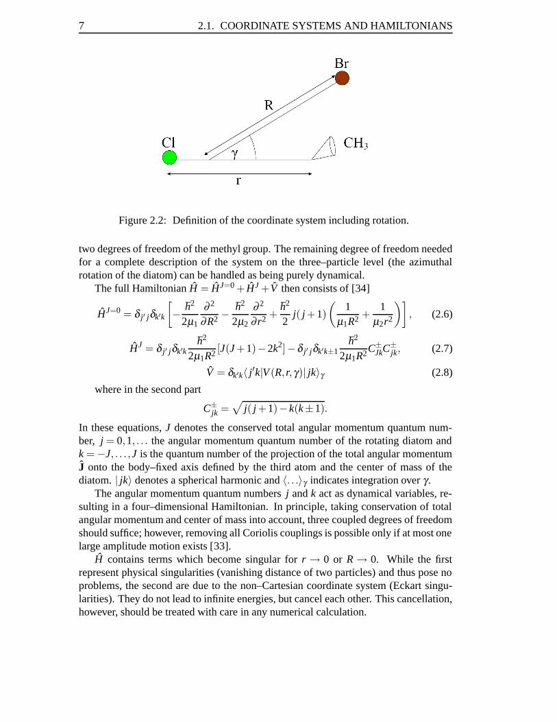
To properly treat the rotation of the diatomic part, we additionally include the angle γdescribing the position of the third particle w.r.t. the diatom (see Fig. 2.2) and omit the
7 2.1. COORDINATE SYSTEMS AND HAMILTONIANS
Figure 2.2: Definition of the coordinate system including rotation.
two degrees of freedom of the methyl group. The remaining degree of freedom neededfor a complete description of the system on the three–particle level (the azimuthalrotation of the diatom) can be handled as being purely dynamical.
The full Hamiltonian H = HJ=0 + HJ +V then consists of [34]
HJ=0 = δ j′ jδk′k
[− h2
2μ1
∂ 2
∂R2 −h2
2μ2
∂ 2
∂ r2 +h2
2j( j +1)
(1
μ1R2 +1
μ2r2
)], (2.6)
HJ = δ j′ jδk′kh2
2μ1R2 [J(J +1)−2k2]−δ j′ jδk′k±1h2
2μ1R2C±JkC
±jk, (2.7)
V = δk′k〈 j′k|V (R,r,γ)| jk〉γ (2.8)
where in the second part
C±jk =
√j( j +1)− k(k±1).
In these equations, J denotes the conserved total angular momentum quantum num-ber, j = 0,1, . . . the angular momentum quantum number of the rotating diatom andk = −J, . . . ,J is the quantum number of the projection of the total angular momentumJ onto the body–fixed axis defined by the third atom and the center of mass of thediatom. | jk〉 denotes a spherical harmonic and 〈. . .〉γ indicates integration over γ .
The angular momentum quantum numbers j and k act as dynamical variables, re-sulting in a four–dimensional Hamiltonian. In principle, taking conservation of totalangular momentum and center of mass into account, three coupled degrees of freedomshould suffice; however, removing all Coriolis couplings is possible only if at most onelarge amplitude motion exists [33].
H contains terms which become singular for r → 0 or R → 0. While the firstrepresent physical singularities (vanishing distance of two particles) and thus pose noproblems, the second are due to the non–Cartesian coordinate system (Eckart singu-larities). They do not lead to infinite energies, but cancel each other. This cancellation,however, should be treated with care in any numerical calculation.
CHAPTER 2. THEORETICAL FRAMEWORK 8
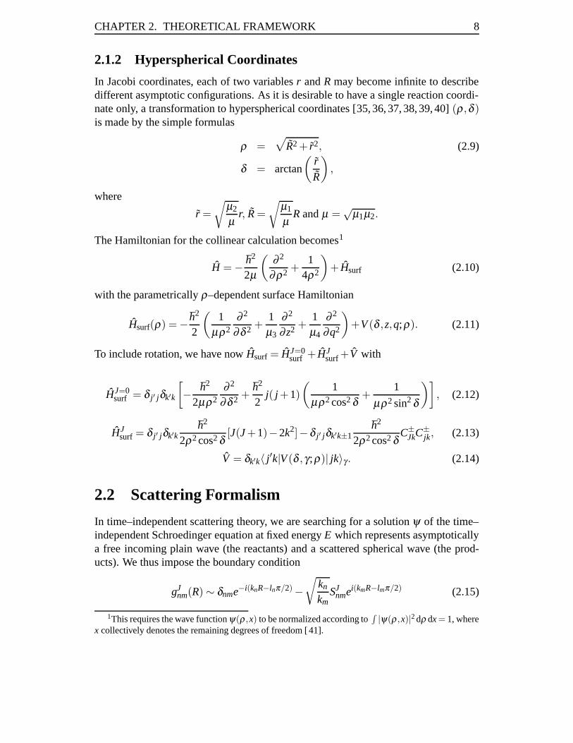
2.1.2 Hyperspherical Coordinates
In Jacobi coordinates, each of two variables r and R may become infinite to describedifferent asymptotic configurations. As it is desirable to have a single reaction coordi-nate only, a transformation to hyperspherical coordinates [35, 36, 37, 38, 39, 40] (ρ,δ )is made by the simple formulas
ρ =√
R2 + r2, (2.9)
δ = arctan
(r
R
),
where
r =√
μ2
μr, R =
√μ1
μR and μ =
√μ1μ2.
The Hamiltonian for the collinear calculation becomes1
H = − h2
2μ
(∂ 2
∂ρ2 +1
4ρ2
)+ Hsurf (2.10)
with the parametrically ρ–dependent surface Hamiltonian
Hsurf(ρ) = − h2
2
(1
μρ2
∂ 2
∂δ 2 +1μ3
∂ 2
∂ z2 +1μ4
∂ 2
∂q2
)+V (δ ,z,q;ρ). (2.11)
To include rotation, we have now Hsurf = HJ=0surf + HJ
surf +V with
HJ=0surf = δ j′ jδk′k
[− h2
2μρ2
∂ 2
∂δ 2 +h2
2j( j +1)
(1
μρ2 cos2 δ+
1
μρ2 sin2 δ
)], (2.12)
HJsurf = δ j′ jδk′k
h2
2ρ2 cos2 δ[J(J +1)−2k2]−δ j′ jδk′k±1
h2
2ρ2 cos2 δC±
JkC±jk, (2.13)
V = δk′k〈 j′k|V (δ ,γ;ρ)| jk〉γ . (2.14)
2.2 Scattering Formalism
In time–independent scattering theory, we are searching for a solution ψ of the time–independent Schroedinger equation at fixed energy E which represents asymptoticallya free incoming plain wave (the reactants) and a scattered spherical wave (the prod-ucts). We thus impose the boundary condition
gJnm(R) ∼ δnme−i(knR−lnπ/2)−
√kn
kmSJ
nmei(kmR−lmπ/2) (2.15)
1This requires the wave function ψ(ρ ,x) to be normalized according to∫ |ψ(ρ ,x)|2 dρ dx = 1, where
x collectively denotes the remaining degrees of freedom [ 41].
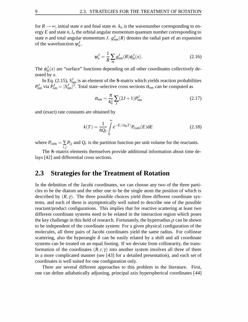
9 2.3. STRATEGIES FOR THE TREATMENT OF ROTATION
for R → ∞, initial state n and final state m. kn is the wavenumber corresponding to en-ergy E and state n, ln the orbital angular momentum quantum number corresponding tostate n and total angular momentum J. gJ
nm(R) denotes the radial part of an expansionof the wavefunction ψJ
n ,
ψJn =
1R ∑
mgJ
nm(R)φ Jm(x). (2.16)
The φ Jm(x) are “surface” functions depending on all other coordinates collectively de-
noted by x.In Eq. (2.15), SJ
nm is an element of the S-matrix which yields reaction probabilitiesPJ
nm via PJnm = |SJ
nm|2. Total state–selective cross sections σnm can be computed as
σnm =πk2
n∑J
(2J +1)PJnm (2.17)
and (exact) rate constants are obtained by
k(T ) =1
hQr
∞∫0
e−E/(kBT )Pcum(E)dE (2.18)
where Pcum = ∑i, j
Pi j and Qr is the partition function per unit volume for the reactants.
The S–matrix elements themselves provide additional information about time de-lays [42] and differential cross sections.
2.3 Strategies for the Treatment of Rotation
In the definition of the Jacobi coordinates, we can choose any two of the three parti-cles to be the diatom and the other one to be the single atom the position of which isdescribed by (R,γ). The three possible choices yield three different coordinate sys-tems, and each of these is asymptotically well suited to describe one of the possiblereactant/product configurations. This implies that for reactive scattering at least twodifferent coordinate systems need to be related in the interaction region which posesthe key challenge in this field of research. Fortunately, the hyperradius ρ can be shownto be independent of the coordinate system: For a given physical configuration of themolecules, all three pairs of Jacobi coordinates yield the same radius. For collinearscattering, also the hyperangle δ can be easily related by a shift and all coordinatesystems can be treated on an equal footing. If we deviate from collinearity, the trans-formation of the coordinates (R,r,γ) into another system involves all three of themin a more complicated manner (see [43] for a detailed presentation), and each set ofcoordinates is well suited for one configuration only.
There are several different approaches to this problem in the literature. First,one can define adiabatically adjusting, principal axis hyperspherical coordinates [44]

CHAPTER 2. THEORETICAL FRAMEWORK 10
which treat all arrangements equivalently. In addition, they can avoid Eckart singu-larities in linear transition state configurations. However, the Hamiltonian contains amixed derivative, and the transformation to Jacobi coordinates needed for the boundarycondition in the asymptotic region is more complicated. Fortunately, for SN2 systems,in the configurations leading to singular terms in the Hamiltonian both halogen atomsare on the same side of the methyl group; therefore, this situation is important forhigh energies only. Other sets of hyperspherical coordinates can be used which arealso less biased towards one of the arrangement configurations (cf. [45]); however,the drawback will be a more complicated transformation to the appropriate asymptoticcoordinates.
Second, the wavefunctions can be computed in different coordinate systems and beconnected by computing an overlap matrix [38]. This requires the choice of referencepotentials which might be critical for a proper description of the interaction region.
In this thesis, we use a third approach to compute the wavefunctions based onone of the (biased) hyperspherical coordinate systems in the interaction region. Thismethod has already been used directly in Jacobi coordinates [54]. By a proper basisset adaptation, we can still accurately describe all arrangement configurations. For anexact Hamiltonian, at fixed hyperradius ρ all arrangement channel coordinates willyield the same eigenstates (with a different parametrization) such that matching ontothe (different) asymptotic coordinate systems is feasible once the interaction region isleft.

Chapter 3
Numerical Methods
This chapter treats the different numerical strategies employed in the calculations. Wefirst outline the solution of the scattering problem after eigenfunctions have been com-puted. The following sections deal with the necessary basis set techniques which arecrucial for a satisfactory performance. As a conceptually complete review could notbe found, the presentation is set to derive the algorithm from general principles oforthogonal polynomials as it was first discovered in [50]. The text should give infor-mation on the efficient implementation of this method and bridge the gap between themathematical and the physical point of view. The last section gives material aboutdiagonalization techniques and possible combinations of these to achieve an improvedperformance for the systems under study.
3.1 R–Matrix Propagation
In solving the scattering problem, we used the technique of R–matrix propagation[46]. The R–matrix relates a matrix valued wavefunction ψnm and its derivatives byRψ ′ = ψ . If such a matrix Rasym is available asymptotically, the S–matrix can beobtained by
S = (RasymO′ −O)−1(RasymI′ − I), (3.1)
where I and O are diagonal matrices representing the incoming and outcoming waves,resp., according to Eq. (2.15). The advantage of using the R–matrix lies in the factthat it is stable and not affected by the exponential behavior of closed (energeticallyforbidden) channels.
For exact results, Rasym needs to be obtained at a large value of the Jacobi coor-dinate R. However, if only reaction probabilities are needed, it is usually sufficient toevaluate the S–matrix directly in hyperspherical coordinates ρ and average [40].
For the construction of Rasym, the reaction coordinate ρ is divided into small sec-tors with midpoints1 ρi. For each ρi, the wavefunction is expanded in a finite product
1This puts some restriction on the distribution of the ρ i and the equations should be rewritten if
CHAPTER 3. NUMERICAL METHODS 12
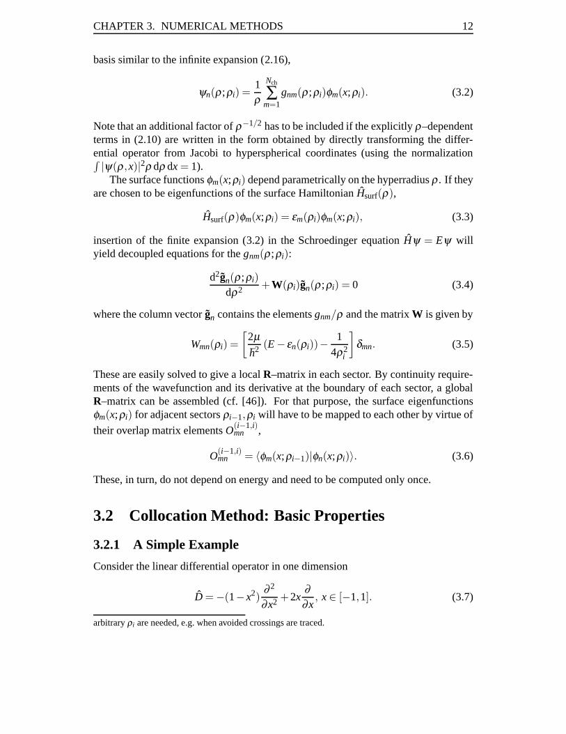
basis similar to the infinite expansion (2.16),
ψn(ρ;ρi) =1ρ
Nch
∑m=1
gnm(ρ;ρi)φm(x;ρi). (3.2)
Note that an additional factor of ρ−1/2 has to be included if the explicitly ρ–dependentterms in (2.10) are written in the form obtained by directly transforming the differ-ential operator from Jacobi to hyperspherical coordinates (using the normalization∫ |ψ(ρ,x)|2ρ dρ dx = 1).
The surface functions φm(x;ρi) depend parametrically on the hyperradius ρ . If theyare chosen to be eigenfunctions of the surface Hamiltonian Hsurf(ρ),
Hsurf(ρ)φm(x;ρi) = εm(ρi)φm(x;ρi), (3.3)
insertion of the finite expansion (3.2) in the Schroedinger equation Hψ = Eψ willyield decoupled equations for the gnm(ρ;ρi):
d2gn(ρ;ρi)dρ2 +W(ρi)gn(ρ;ρi) = 0 (3.4)
where the column vector gn contains the elements gnm/ρ and the matrix W is given by
Wmn(ρi) =[
2μh2 (E − εn(ρi))− 1
4ρ2i
]δmn. (3.5)
These are easily solved to give a local R–matrix in each sector. By continuity require-ments of the wavefunction and its derivative at the boundary of each sector, a globalR–matrix can be assembled (cf. [46]). For that purpose, the surface eigenfunctionsφm(x;ρi) for adjacent sectors ρi−1,ρi will have to be mapped to each other by virtue of
their overlap matrix elements O(i−1,i)mn ,
O(i−1,i)mn = 〈φm(x;ρi−1)|φn(x;ρi)〉. (3.6)
These, in turn, do not depend on energy and need to be computed only once.
3.2 Collocation Method: Basic Properties
3.2.1 A Simple Example
Consider the linear differential operator in one dimension
D = −(1− x2)∂ 2
∂x2 +2x∂∂x
, x ∈ [−1,1]. (3.7)
arbitrary ρi are needed, e.g. when avoided crossings are traced.
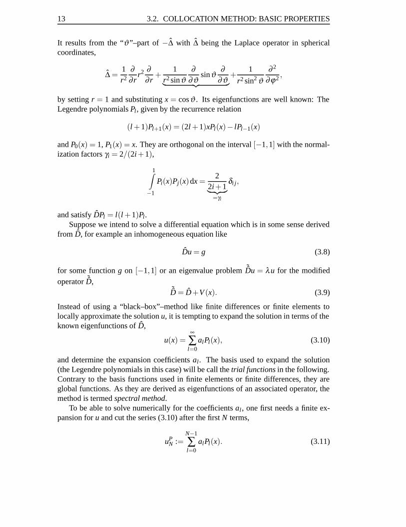
13 3.2. COLLOCATION METHOD: BASIC PROPERTIES
It results from the “ϑ”–part of −Δ with Δ being the Laplace operator in sphericalcoordinates,
Δ =1r2
∂∂ r
r2 ∂∂ r
+1
r2 sinϑ∂
∂ϑsinϑ
∂∂ϑ︸ ︷︷ ︸+
1
r2 sin2 ϑ∂ 2
∂ϕ2 ,
by setting r = 1 and substituting x = cosϑ . Its eigenfunctions are well known: TheLegendre polynomials Pl, given by the recurrence relation
(l +1)Pl+1(x) = (2l +1)xPl(x)− lPl−1(x)
and P0(x) = 1, P1(x) = x. They are orthogonal on the interval [−1,1] with the normal-ization factors γi = 2/(2i+1),
1∫−1
Pi(x)Pj(x)dx =2
2i+1︸ ︷︷ ︸=γi
δi j,
and satisfy DPl = l(l +1)Pl.Suppose we intend to solve a differential equation which is in some sense derived
from D, for example an inhomogeneous equation like
Du = g (3.8)
for some function g on [−1,1] or an eigenvalue problem ˜Du = λu for the modifiedoperator ˜D,
˜D = D+V (x). (3.9)
Instead of using a “black–box”–method like finite differences or finite elements tolocally approximate the solution u, it is tempting to expand the solution in terms of theknown eigenfunctions of D,
u(x) =∞
∑l=0
alPl(x), (3.10)
and determine the expansion coefficients al. The basis used to expand the solution(the Legendre polynomials in this case) will be call the trial functions in the following.Contrary to the basis functions used in finite elements or finite differences, they areglobal functions. As they are derived as eigenfunctions of an associated operator, themethod is termed spectral method.
To be able to solve numerically for the coefficients al , one first needs a finite ex-pansion for u and cut the series (3.10) after the first N terms,
uPN :=
N−1
∑l=0
alPl(x). (3.11)

CHAPTER 3. NUMERICAL METHODS 14
Formally, uPN is obtained by applying a projection operator PN to u, PNu = uP
N , wherePN will project each continuous function onto the first N Legendre polynomials, i.e. inDirac notation
PN :=N−1
∑l=0
|Pl ><Pl|. (3.12)
The efficiency of the method will depend on the convergence speed of the expansion(3.10) which, in turn, is determined by the decay rate of the expansion coefficients al.In the next section, we can see in a quite general setting that our ansatz is promising.
3.2.2 Spectral Accuracy
Suppose we have some linear differential operator ˜D and we would like to solve adifferential equation
˜Du = g. (3.13)
If we know the eigenfunctions φk of a “similar” operator D,
Dφk = λkφk, (3.14)
then it is reasonable to expand the solution u of the differential equation (3.13) in termsof the φk:
u = ∑k
ukφk. (3.15)
If the eigenfunctions of D are orthonormal w.r.t. a scalar product (,), the expansioncoefficients uk are obtained from uk = (u,φk). Now, if the operator is hermitian, wecan write
uk = (u,φk) =1λk
(u, Dφk) =1λk
(Du,φk)
and by iteration
uk =1
λ mk
(Dmu,φk)
for every m ≥ 1. If Dmu is still “well–behaved”, i.e. ‖Dmu‖ exists, we get by Cauchy–Schwarz the inequality
|uk| ≤ 1|λk|m‖Dmu‖. (3.16)
If the eigenvalues λk grow at least like kα , α > 0 (which is the case for the usualorthogonal polynomials) and ‖Dmu‖ remains bounded for m → ∞, the expansion co-efficients |uk| will decay faster than any inverse power of k (exponential convergence,spectral accuracy).
The main assumptions made in this argument concern the hermiticity of the op-erator D and the growth of ‖Dmu‖. The first assumption can be closely related toappropriate boundary conditions if we think in terms of partial integration. For the

15 3.2. COLLOCATION METHOD: BASIC PROPERTIES
second, note that the expansion coefficients uk can be linked to the difference D− ˜Dof the operators D and ˜D and also to the expansion coefficients of g:
uk = (u,φk) =1λk
(Du,φk) =1λk
(((D− ˜D)+ ˜D)u,φk
)=
1λk
((D− ˜D)u+g,φk
).
In general, spectral accuracy is an asymptotic statement for large k, i.e. it need notimply an efficient numerical behavior. However, if the trial functions φk are chosenproperly, fast convergence will in practice often be achieved [47, 67]. An example isgiven in Sec. 3.4.3. In theory, the expansion coefficients of Tschebyscheff series ofentire functions converge to zero even faster than exponential; in case of singularitiesoff the real line, the convergence is exponential, and with singularities in the domain ofdefinition [−1,1], only algebraic convergence is achieved (see [48] for a brief summaryand further references).
3.2.3 Generating a Matrix Representation
To generate a numerical solution for our examples in Eq. (3.8) or (3.9), resp., we willsubstitute u by the finite expansion uP
N , Eq. (3.11),
DuPN(x) ≈ g(x), (3.17)
or(D+V (x))uP
N(x) ≈ λuPN(x), (3.18)
and then solve for the expansion coefficients al, l = 0, . . . ,N − 1. For this purpose,additional procedures have to be invented to reduce each remaining trial function toa finite set and to ensure that the approximate solution will satisfy the differentialequation as closely as possible. The various choices for minimizing the residual errorwill create the difference between one spectral method and another. In general, theobtained solutions al, l = 0, . . . ,N −1 will differ from the coefficients al in the exactsolution and depend on the procedure invented.
One possibility is to form matrix elements with test functions and solve the result-ing matrix equation or matrix eigenvalue problem, respectively. If we use the trialfunctions as test functions, the approach is called Galerkin in the context of fluiddynamics [47], variational or a Variational Basis Representation (VBR) in quantummechanics [60]. (The procedure is essentially the same as for finite elements, the dif-ference lies in the choice of the functions.) We obtain a system of linear equations forthe expansion coefficients al which in matrix form reads for (3.17)
Dlmam = gl (3.19)
CHAPTER 3. NUMERICAL METHODS 16
with
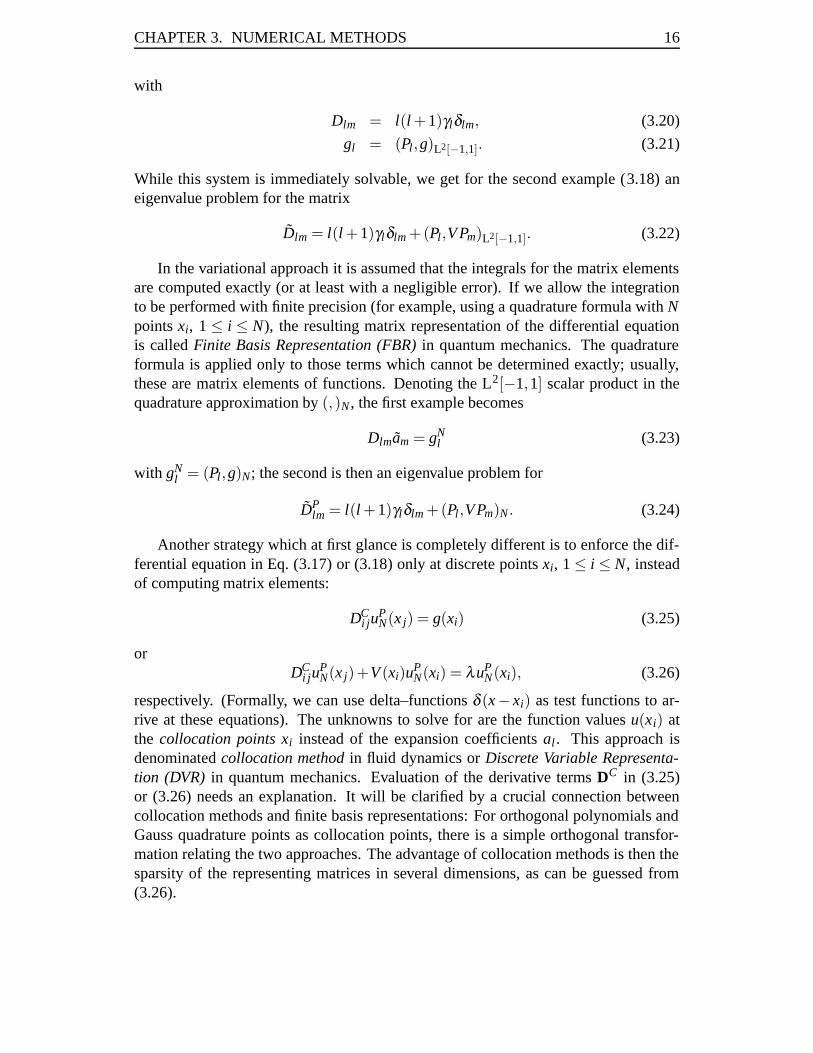
Dlm = l(l +1)γlδlm, (3.20)
gl = (Pl,g)L2[−1,1]. (3.21)
While this system is immediately solvable, we get for the second example (3.18) aneigenvalue problem for the matrix
Dlm = l(l +1)γlδlm +(Pl,VPm)L2[−1,1]. (3.22)
In the variational approach it is assumed that the integrals for the matrix elementsare computed exactly (or at least with a negligible error). If we allow the integrationto be performed with finite precision (for example, using a quadrature formula with Npoints xi, 1 ≤ i ≤ N), the resulting matrix representation of the differential equationis called Finite Basis Representation (FBR) in quantum mechanics. The quadratureformula is applied only to those terms which cannot be determined exactly; usually,these are matrix elements of functions. Denoting the L2[−1,1] scalar product in thequadrature approximation by (,)N , the first example becomes
Dlmam = gNl (3.23)
with gNl = (Pl,g)N; the second is then an eigenvalue problem for
DPlm = l(l +1)γlδlm +(Pl,VPm)N. (3.24)
Another strategy which at first glance is completely different is to enforce the dif-ferential equation in Eq. (3.17) or (3.18) only at discrete points xi, 1 ≤ i ≤ N, insteadof computing matrix elements:
DCi ju
PN(x j) = g(xi) (3.25)
orDC
i juPN(x j)+V (xi)uP
N(xi) = λuPN(xi), (3.26)
respectively. (Formally, we can use delta–functions δ (x− xi) as test functions to ar-rive at these equations). The unknowns to solve for are the function values u(xi) atthe collocation points xi instead of the expansion coefficients al . This approach isdenominated collocation method in fluid dynamics or Discrete Variable Representa-tion (DVR) in quantum mechanics. Evaluation of the derivative terms DC in (3.25)or (3.26) needs an explanation. It will be clarified by a crucial connection betweencollocation methods and finite basis representations: For orthogonal polynomials andGauss quadrature points as collocation points, there is a simple orthogonal transfor-mation relating the two approaches. The advantage of collocation methods is then thesparsity of the representing matrices in several dimensions, as can be guessed from(3.26).
17 3.3. COLLOCATION METHOD AND ORTHOGONAL POLYNOMIALS
3.3 Collocation Method and Orthogonal Polynomials
3.3.1 Orthogonal Polynomials
Collocations methods can be best understood in the framework of orthogonal polyno-mials. For this reason we first collect some properties of these, following [51].
Basic Properties
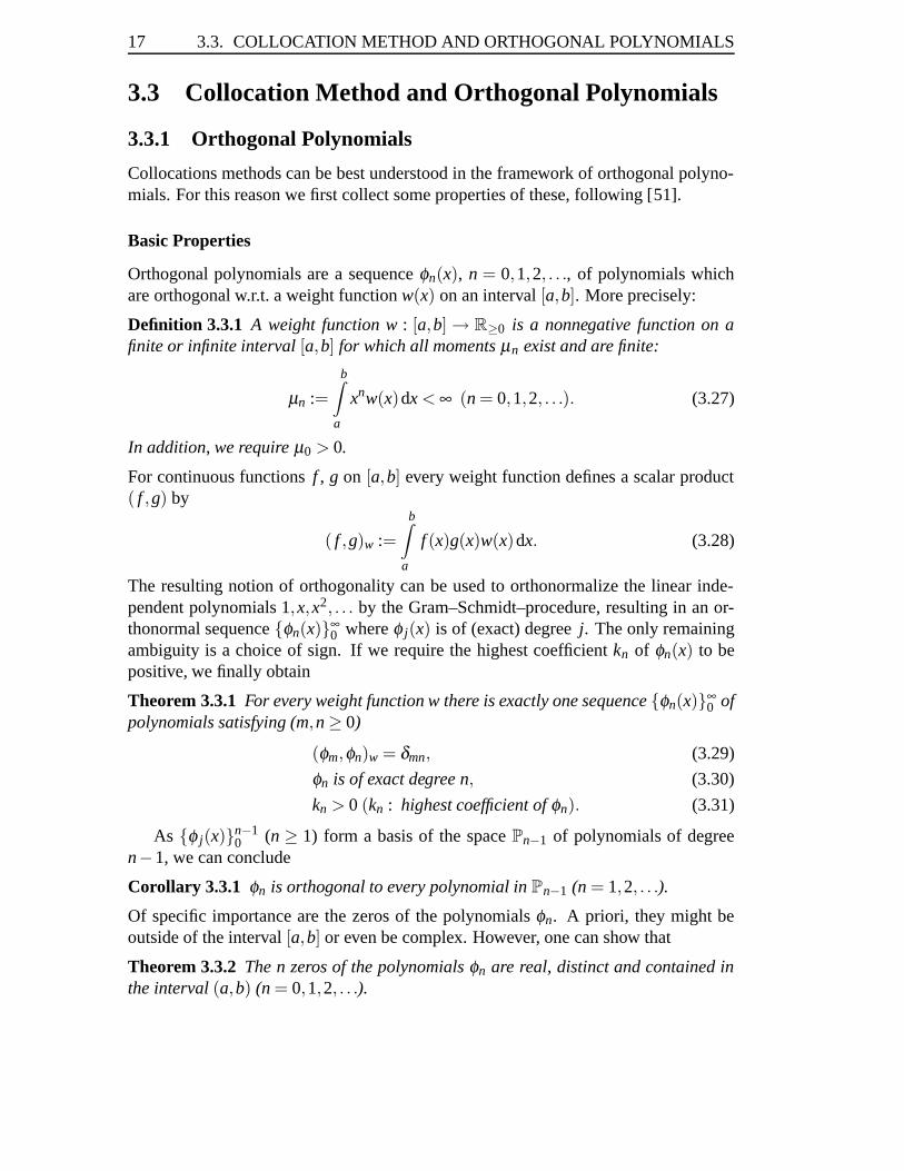
Orthogonal polynomials are a sequence φn(x), n = 0,1,2, . . ., of polynomials whichare orthogonal w.r.t. a weight function w(x) on an interval [a,b]. More precisely:
Definition 3.3.1 A weight function w : [a,b] → R≥0 is a nonnegative function on afinite or infinite interval [a,b] for which all moments μn exist and are finite:
μn :=b∫
a
xnw(x)dx < ∞ (n = 0,1,2, . . .). (3.27)
In addition, we require μ0 > 0.
For continuous functions f , g on [a,b] every weight function defines a scalar product( f ,g) by
( f ,g)w :=b∫
a
f (x)g(x)w(x)dx. (3.28)
The resulting notion of orthogonality can be used to orthonormalize the linear inde-pendent polynomials 1,x,x2, . . . by the Gram–Schmidt–procedure, resulting in an or-thonormal sequence {φn(x)}∞
0 where φ j(x) is of (exact) degree j. The only remainingambiguity is a choice of sign. If we require the highest coefficient kn of φn(x) to bepositive, we finally obtain
Theorem 3.3.1 For every weight function w there is exactly one sequence {φn(x)}∞0 of
polynomials satisfying (m,n ≥ 0)
(φm,φn)w = δmn, (3.29)
φn is of exact degree n, (3.30)
kn > 0 (kn : highest coefficient of φn). (3.31)
As {φ j(x)}n−10 (n ≥ 1) form a basis of the space Pn−1 of polynomials of degree
n−1, we can conclude
Corollary 3.3.1 φn is orthogonal to every polynomial in Pn−1 (n = 1,2, . . .).
Of specific importance are the zeros of the polynomials φn. A priori, they might beoutside of the interval [a,b] or even be complex. However, one can show that
Theorem 3.3.2 The n zeros of the polynomials φn are real, distinct and contained inthe interval (a,b) (n = 0,1,2, . . .).
CHAPTER 3. NUMERICAL METHODS 18
Recurrence Relation
In a sequence {φ j(x)}∞0 of orthogonal polynomials, each φn(x) (n ≥ 1) can be ex-
pressed as a linear combination of φ0(x), . . . ,φn−1(x) and xφn−1(x). However, due tothe orthogonality property of each φn to all polynomials of lower degree (corollary3.3.1), none of the φ j(x) with j < n−2 are needed:
Theorem 3.3.3 Every sequence {φ j(x)}∞0 of orthogonal polynomials satisfies a three–
term–recurrence of the form (n ≥ 2)
φn(x) =(
kn
kn−1x+Bn
)φn−1(x)− knkn−2
k2n−1
φn−2(x), Bn ∈ R. (3.32)
Note that this form requires the polynomials to be normalized according to (3.29). Ifwe set φ−1 ≡ 0, it extends to n = 1.
Jacobi Matrix
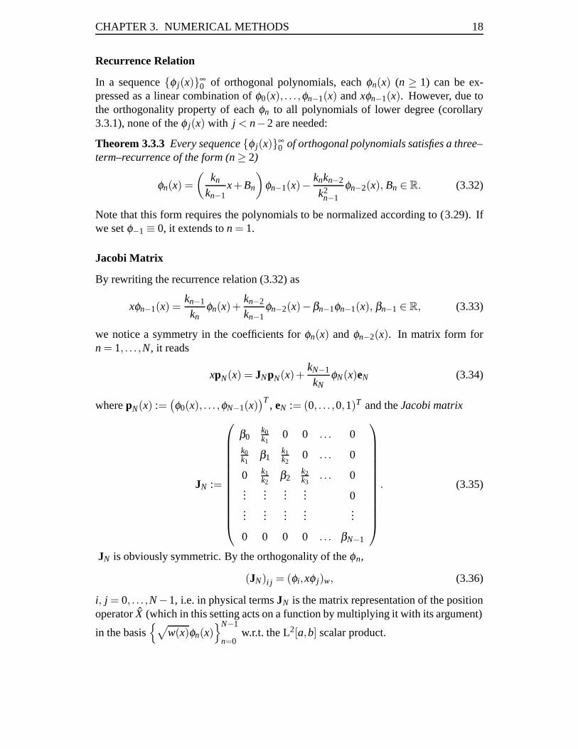
By rewriting the recurrence relation (3.32) as
xφn−1(x) =kn−1
knφn(x)+
kn−2
kn−1φn−2(x)−βn−1φn−1(x), βn−1 ∈ R, (3.33)
we notice a symmetry in the coefficients for φn(x) and φn−2(x). In matrix form forn = 1, . . . ,N, it reads
xpN(x) = JNpN(x)+kN−1
kNφN(x)eN (3.34)
where pN(x) :=(φ0(x), . . . ,φN−1(x)
)T, eN := (0, . . . ,0,1)T and the Jacobi matrix
JN :=
⎛⎜⎜⎜⎜⎜⎜⎜⎜⎜⎜⎜⎜⎝
β0k0k1
0 0 . . . 0k0k1
β1k1k2
0 . . . 0
0 k1k2
β2k2k3
. . . 0...
......
... 0...
......
......
0 0 0 0 . . . βN−1
⎞⎟⎟⎟⎟⎟⎟⎟⎟⎟⎟⎟⎟⎠
. (3.35)
JN is obviously symmetric. By the orthogonality of the φn,
(JN)i j = (φi,xφ j)w, (3.36)
i, j = 0, . . . ,N−1, i.e. in physical terms JN is the matrix representation of the positionoperator X (which in this setting acts on a function by multiplying it with its argument)
in the basis{√
w(x)φn(x)}N−1
n=0w.r.t. the L2[a,b] scalar product.
19 3.3. COLLOCATION METHOD AND ORTHOGONAL POLYNOMIALS
Christoffel–Darboux–Identity
The matrix form (3.34) of the recurrence relation enables us to establish an explicitexpression for “scalar products” of polynomials with fixed arguments which will becrucial in the following:
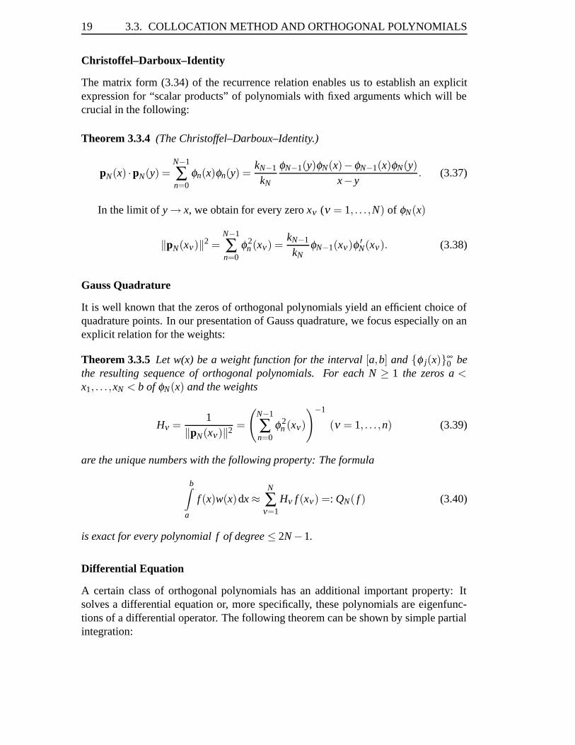
Theorem 3.3.4 (The Christoffel–Darboux–Identity.)
pN(x) ·pN(y) =N−1
∑n=0
φn(x)φn(y) =kN−1
kN
φN−1(y)φN(x)−φN−1(x)φN(y)x− y
. (3.37)
In the limit of y → x, we obtain for every zero xν (ν = 1, . . . ,N) of φN(x)
‖pN(xν)‖2 =N−1
∑n=0
φ 2n (xν) =
kN−1
kNφN−1(xν)φ ′
N(xν). (3.38)
Gauss Quadrature
It is well known that the zeros of orthogonal polynomials yield an efficient choice ofquadrature points. In our presentation of Gauss quadrature, we focus especially on anexplicit relation for the weights:
Theorem 3.3.5 Let w(x) be a weight function for the interval [a,b] and {φ j(x)}∞0 be
the resulting sequence of orthogonal polynomials. For each N ≥ 1 the zeros a <x1, . . . ,xN < b of φN(x) and the weights
Hν =1
‖pN(xν)‖2 =
(N−1
∑n=0
φ 2n (xν)
)−1
(ν = 1, . . . ,n) (3.39)
are the unique numbers with the following property: The formula
b∫a
f (x)w(x)dx ≈N
∑ν=1
Hν f (xν) =: QN( f ) (3.40)
is exact for every polynomial f of degree ≤ 2N −1.
Differential Equation
A certain class of orthogonal polynomials has an additional important property: Itsolves a differential equation or, more specifically, these polynomials are eigenfunc-tions of a differential operator. The following theorem can be shown by simple partialintegration:
CHAPTER 3. NUMERICAL METHODS 20
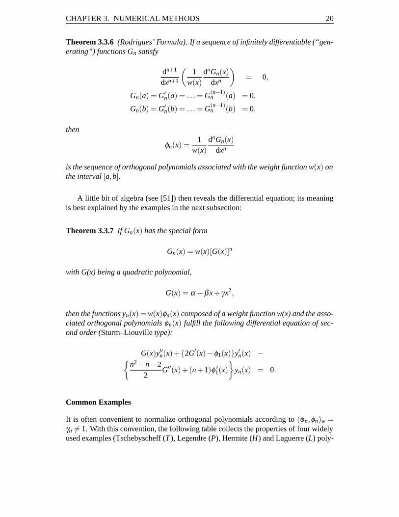
Theorem 3.3.6 (Rodrigues’ Formula). If a sequence of infinitely differentiable (“gen-erating”) functions Gn satisfy
dn+1
dxn+1
(1
w(x)dnGn(x)
dxn
)= 0,
Gn(a) = G′n(a) = . . . = G(n−1)
n (a) = 0,
Gn(b) = G′n(b) = . . . = G(n−1)
n (b) = 0,
then
φn(x) =1
w(x)dnGn(x)
dxn
is the sequence of orthogonal polynomials associated with the weight function w(x) onthe interval [a,b].
A little bit of algebra (see [51]) then reveals the differential equation; its meaningis best explained by the examples in the next subsection:
Theorem 3.3.7 If Gn(x) has the special form
Gn(x) = w(x)[G(x)]n
with G(x) being a quadratic polynomial,
G(x) = α +βx+ γx2,
then the functions yn(x) = w(x)φn(x) composed of a weight function w(x) and the asso-ciated orthogonal polynomials φn(x) fulfill the following differential equation of sec-ond order (Sturm–Liouville type):
G(x)y′′n(x)+{2G′(x)−φ1(x)}y′n(x) −{n2 −n−2
2G′′(x)+(n+1)φ ′
1(x)}
yn(x) = 0.
Common Examples
It is often convenient to normalize orthogonal polynomials according to (φn,φn)w =γn �= 1. With this convention, the following table collects the properties of four widelyused examples (Tschebyscheff (T ), Legendre (P), Hermite (H) and Laguerre (L) poly-
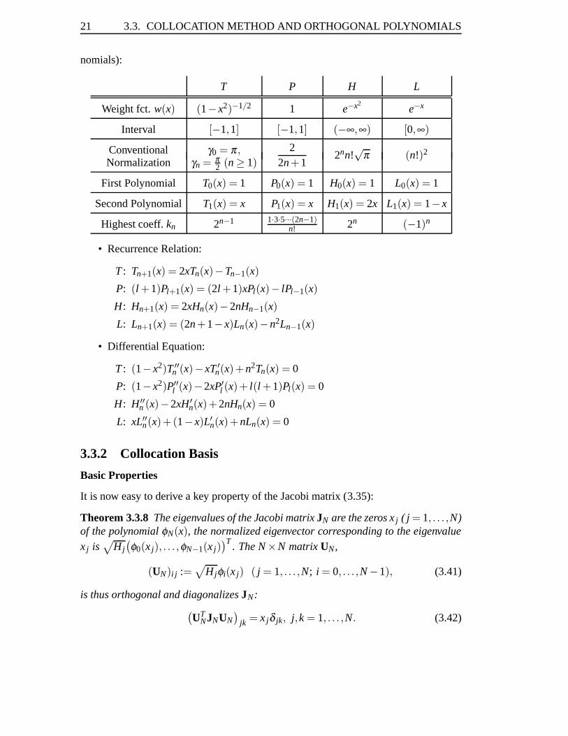
21 3.3. COLLOCATION METHOD AND ORTHOGONAL POLYNOMIALS
nomials):
T P H L
Weight fct. w(x) (1− x2)−1/2 1 e−x2e−x
Interval [−1,1] [−1,1] (−∞,∞) [0,∞)
Conventional γ0 = π,Normalization γn = π
2 (n ≥ 1)2
2n+12nn!
√π (n!)2
First Polynomial T0(x) = 1 P0(x) = 1 H0(x) = 1 L0(x) = 1
Second Polynomial T1(x) = x P1(x) = x H1(x) = 2x L1(x) = 1− x
Highest coeff. kn 2n−1 1·3·5···(2n−1)n! 2n (−1)n
• Recurrence Relation:
T : Tn+1(x) = 2xTn(x)−Tn−1(x)
P: (l +1)Pl+1(x) = (2l +1)xPl(x)− lPl−1(x)
H: Hn+1(x) = 2xHn(x)−2nHn−1(x)
L: Ln+1(x) = (2n+1− x)Ln(x)−n2Ln−1(x)
• Differential Equation:
T : (1− x2)T ′′n (x)− xT ′
n(x)+n2Tn(x) = 0
P: (1− x2)P′′l (x)−2xP′
l (x)+ l(l +1)Pl(x) = 0
H: H ′′n (x)−2xH ′
n(x)+2nHn(x) = 0
L: xL′′n(x)+(1− x)L′
n(x)+nLn(x) = 0
3.3.2 Collocation Basis
Basic Properties
It is now easy to derive a key property of the Jacobi matrix (3.35):
Theorem 3.3.8 The eigenvalues of the Jacobi matrix JN are the zeros x j ( j = 1, . . . ,N)of the polynomial φN(x), the normalized eigenvector corresponding to the eigenvalue
x j is√
Hj(φ0(x j), . . . ,φN−1(x j)
)T. The N ×N matrix UN,
(UN)i j :=√
Hjφi(x j) ( j = 1, . . . ,N; i = 0, . . . ,N −1), (3.41)
is thus orthogonal and diagonalizes JN:(UT
NJNUN)
jk = x jδ jk, j,k = 1, . . . ,N. (3.42)
CHAPTER 3. NUMERICAL METHODS 22
Proof: From (3.34), we obtain by substituting a zero x j for x
x jpN(x j) = JNpN(x j),
i e.(φ0(x j), . . . ,φN−1(x j)
)Tis eigenvector of JN corresponding to the eigenvalue x j.
The normalization of the rows and columns, resp., of UN follows from the explicitformula (3.39) for the weights of the associated Gauss quadrature. �
While the properties (3.41) and (3.42) are interesting in themselves and providea numerically stable algorithm to compute roots and weights for a Gauss quadra-ture [55, 56], their importance extend to the option of performing orthogonal basistransformations via the matrix UN [50]. In particular, we can apply this transforma-tion to the orthogonal basis {φn(x)}N−1
n=0 of the space PN−1 of polynomials with degree≤ N −1:
Definition 3.3.2 For every sequence {φn(x)}∞n=0 and every N ≥ 1, the associated col-
location basis is given by
ψNn :=
(UT
NpN
)n (n = 1, . . . ,N). (3.43)
Note that the collocation basis depends on N in the sense that – contrary to the orthog-onal polynomials – enlarging the basis will not simply add another basis function, butchange all of them. The shape of these functions is clarified by
Theorem 3.3.9 Every collocation basis{
ψNn
}N−1n=0 associated to a weight function
w(x) on an interval [a,b] has the following properties (m,n ≥ 0, f any continuousfunction):
(ψNm ,ψN
n )w = δmn, (3.44)
ψNn (xm) =
1√Hn
δmn, (3.45)
(ψNn , f )w ≈ QN(ψN
m f ) =√
Hn f (xn), (3.46)
(ψNm , f ψN
n )w ≈ QN(ψNm f ψN
n ) = f (xn)δmn. (3.47)
Proof: The first statement immediately follows from the orthogonality of UN and theorthonormality (3.29) of the orthogonal polynomials φn(x). For the second, note theexplicit formula
ψNn (x) =
√Hn
N−1
∑i=0
φi(xn)φi(x) (3.48)
and the orthonormality of the columns of UN . The third and fourth are easy conse-quences then; the latter, for example, follows from
(ψNm , f ψN
n )w =b∫
a
ψNm (x) f (x)ψN
n (x)w(x)dx
23 3.3. COLLOCATION METHOD AND ORTHOGONAL POLYNOMIALS
≈ QN(ψNm f ψN
n )
=N
∑ν=1
HνψNm (xν) f (xν)ψN
n (xν)
=N
∑ν=1
Hνδmν1√Hm
f (xν)δnν1√Hn
= f (xn)δmn.
�
Eq. (3.45) reveals the collocation basis to be suitably weighted Lagrange polyno-mials for the roots of the relevant Gauss quadrature,
ψNn (x) =
1√Hn
N
∏i=1i�=k
x− xi
xn− xi. (3.49)
(In particular, each ψNn (x) is a polynomial of (exact) degree N −1). In this sense, the
collocation points xi themselves can be regarded as the basis (instead of viewing themas simple technical quantities needed to evaluate integrals), and the mesh created bythem is called a Lagrange Mesh [57].
Algorithm
Of special interest is the last property (3.47) as it yields a diagonal matrix representa-tion for terms without derivatives in a partial differential equation. In the case of anoperator D containing derivatives, the corresponding matrix elements in the colloca-tion basis are
DCi j = (ψN
i , DψNj )w. (3.50)
They can either be computed directly (based on the explicit formula (3.49) for thebasis functions) or be evaluated in the basis of orthogonal polynomials (where theyoften have a simple shape, cf. (3.20)),
DPi j = (φi, Dφ j)w, (3.51)
and then transformed via the matrix UN:
DC = UNDPUTN. (3.52)
The algorithm to approximately solve a linear differential equation (cf. (3.8)) or eigen-value problem of a differential operator (cf. (3.9)) for uP
N in the collocation method canbe summarized as follows:
1. Choose an appropriate basis of orthogonal polynomials φn2 and the basis size N.
2A generally useful choice is provided by the Tschebyscheff polynomials, see Sec. 3.4.2.
CHAPTER 3. NUMERICAL METHODS 24
2. Set up the Jacobi matrix JN (3.35) with the coefficients kn, βn from the normal-ized recursion relation (3.33).
3. Diagonalize JN as in (3.42) to obtain the transformation matrix UN and colloca-tion points xi.
4. Set up the problem in the collocation basis:
(a) Derivatives: Transform by (3.52) from the finite basis representation orcompute directly using (3.49);
(a) Functions as multiplicative operators: Evaluate at the collocation pointsaccording to (3.47), yielding a diagonal matrix representation;
(a) Functions g as vectors on the right hand side: Evaluate pointwise in eachentry as
√Hig(xi), see (3.46).
5. Solve the resulting matrix problem. The solution vector(s) u contain√
HiuPN(xi)
as entries, see (3.45).
In our examples (3.8) and (3.9), the diagonal entries in the Jacobi matrix JN are βi = 0(see Sec. 3.3.1). For the off-diagonal ones, note that the sequence needs to be normal-ized by φl = Pl/
√γl . The highest coefficient of the polynomial φl is then kl/√γl and
the matrix entries turn out to be
(JN)i j =
⎧⎪⎪⎪⎪⎨⎪⎪⎪⎪⎩
i√4i2 −1
for i = j−1,
j√4 j2 −1
for j = i−1,
0 otherwise.
(3.53)
After transforming the derivative matrix DPlm = l(l +1)δlm in the collocation basis via
(3.52) to yield DC, we finally get the matrix equation
DCu = g (3.54)
with gi =√
Hig(xi) or the matrix eigenvalue problem for
DC +V (3.55)
with Vi j = V (xi)δi j. (Note that both (3.25) and (3.26) imply a different normalization).
25 3.3. COLLOCATION METHOD AND ORTHOGONAL POLYNOMIALS
Convergence Properties
• Convergence of the Expansion
For a sequence of orthogonal polynomials {φn(x)}∞0 and a function f , we can try to
expand the function in terms of the polynomials, i.e.
f (x) ∼∞
∑n=0
cnφn(x) (3.56)
with
cn = (φ , f )w =b∫
a
φn(x) f (x)w(x)dx. (3.57)
While the general answer to the problem of what ∼ means in (3.56) opens up the fieldof approximation theory which shall not be considered here, an interesting statementcan be given for the case that a and b are finite [61] (similar to the Dini–Lipschitz testfor the pointwise convergence of Fourier–series):
Theorem 3.3.10 Let f be continuous on the finite interval [a,b] and satisfy a Lipschitz–condition at x0, i.e. | f (x)− f (x0)| ≤ K|x− x0| for some K > 0. Suppose in additionthat φn(x0) remains bounded for n → ∞. Then (3.56) holds pointwise at x0.
Proof: The partial sum SN(x) is
SN(x0) =N
∑n=0
(φ , f )wφn(x0)
=N
∑n=0
b∫a
φn(y) f (y)w(y)dy φn(x0)
=b∫
a
f (y)w(y)
(N
∑n=0
φn(x0)φn(y)
)dy.
For the term in brackets, we can insert the Christoffel–Darboux–Identity (3.37). Bymultiplying this identity with w(y) and integrating over y, we get by orthogonality
1 =kN
kN+1
b∫a
φN(y)φN+1(x0)−φN(x0)φN+1(y)x0 − y
w(y)dy.
After multiplying with f (x0) and subtracting from SN(x0), we obtain for the difference
SN(x0)− f (x0) =
kN
kN+1
b∫a
[ f (y)− f (x0)]φN(y)φN+1(x0)−φN(x0)φN+1(y)
x0 − yw(y)dy.
CHAPTER 3. NUMERICAL METHODS 26
The fraction kN/kN+1 can be estimated to remain bounded: It is an entry of the Jacobimatrix the eigenvalues of which are the zeros of φN and thus lie in the finite interval[a,b]; as the diagonal entries βn are positive, kN/kN+1 is bounded by the largest zeroxmax as can be seen with a suitably chosen test vector x in
xmax ≥ (x,JNx)(x,x)
.
Therefore it remains to show that the integral tends to zero. The expression can berewritten as
SN(x0)− f (x0) =kN
kN+1
((h,φN+1)wφN(x0)− (h,φN)wφN+1(x0)
)where h(y) = ( f (y)− f (x0))/(y−x0). By the Lipschitz–condition for f , h is boundedand continuous (except, possibly, at x0); the numbers (h,φN)w as the generalizedFourier coefficients of h thus tend to zero for N → ∞. As φN(x0) remains bounded,the total right hand side vanishes for N → ∞. �
• Error Classification
The principle error in every spectral method will be caused by using only a finiteexpansion uP
N like (3.11) to generate the approximate solution. As pointed out inthe introduction, Sec. 3.2.3, the expansion coefficients uN
k in the numerical solutionwill depend on N itself. In other words, if u is a solution for a differential equationlike Du = g, then PNu, the solution projected onto the first N orthogonal polynomials(with PN as in (3.12)), will in general not be a solution of the reduced matrix equationPNDPNu = PNg. However, the difference u− PNu between the exact and the projectedsolution can serve to analyze the error by looking at its norm,
‖u− PNu‖w, (3.58)
where ‖ · ‖w is derived from the scalar product (,)w.A second type of error arises from the approximate evaluation of the matrix el-
ements by (Gauss) quadrature. Note that this error is the same for the collocationmethod and the finite basis representation which are related by an orthogonal transfor-mation. To shed more light on this error, we exploit the special integration property(3.47) of the collocation basis to define an adapted discrete scalar product [47]:
Definition 3.3.3 For any two continuous functions f , g on [a,b], we define
( f ,g)N := QN( f g) =N
∑ν=1
Hν f (xν)g(xν). (3.59)

27 3.3. COLLOCATION METHOD AND ORTHOGONAL POLYNOMIALS
For two polynomials f , g the product of which has a degree of at most 2N −1, we get
( f ,g)N = ( f ,g)w (3.60)
by the Gaussian integration property (3.40). Thus, (,)N is a scalar product on thespace PN−1 of polynomials of degree ≤ N−1 and we have orthonormality of the finitepolynomial basis φn for n = 0, . . . ,N−1 and the collocation basis ψN
n for n = 1, . . . ,N:
(φn,φm)N = (ψNn ,ψN
m )N = δmn. (3.61)
The collocation aims at finding the values u(xi) of the solution u at the collocationpoints. If we again neglect the fact that the numerically obtained values will differ fromthe exact ones for finite N, the collocation solution can essentially be described by aninterpolation polynomial INu of degree N −1 which agrees with the exact solution inall xi:
(INu)(xi) = u(xi), 1 ≤ i ≤ N, INu ∈ PN−1. (3.62)
(The additional factor√
Hi contained in the solution vectors is not relevant for thisanalysis). In terms of the finite basis φn, we can write
INu =N−1
∑i=0
uiφi
with the discrete polynomial coefficients ui; their difference to the expansion coeffi-cients describes the quadrature error. For every continuous f , we have
(INu, f )N = (u, f )N, (3.63)
i.e. INu is the projection of u onto PN−1 w.r.t. the discrete scalar product (,)N , whereasPNu projects w.r.t. (,)w. As a consequence, we can compute the discrete polynomialcoefficients from
ui = (u,φi)N,
and by (3.61) we can express them as
ui =
(∞
∑k=0
ukφk,φi
)N
= ui +∞
∑k=N
(φk,φi)Nuk.
Multiplying with φi and summing from i = 0 to N −1, this reads
INu = PNu+ RNu (3.64)
with the quadrature error or aliasing error
RNu :=N−1
∑i=0
(∞
∑k=N
(φk,φi)Nuk
)φi. (3.65)

CHAPTER 3. NUMERICAL METHODS 28
Now RNu is orthogonal to u− PNu w.r.t. (,)w as the former is a linear combination ofpolynomials φi up to index N −1 and the latter starts at index N. Therefore
‖u− INu‖2w = ‖u− PNu‖2
w +‖RNu‖2w. (3.66)
By (3.65), the additional error ‖RNu‖2w is caused by quadrature instead of exact inte-
gration and will crucially depend on the decay of the expansion coefficients uk which,in case of spectral accuracy, can be expected to be faster than polynomial.
• Spectral Accuracy Revisited
A qualitative argument in addition to the one given in Sec. 3.2.2 might support theexpected fast convergence of the method [63]. In the analysis of the convergenceproperties of finite differences or finite elements, the error is usually of the form O(hα),where h refers to the spacing of the points and α > 0 depends on the method chosen,i.e. the polynomial degree. For collocation methods, increasing the size N of the basiswill both decrease the grid spacing h≈ 1/N and increase the polynomial degree N ≈α ,so that the resulting error is
≈ O[(1/N)N],
i.e. it decreases faster than any finite power of N.
3.4 Generalizations
3.4.1 Several Dimensions
Passing from one to d dimensions (and thus from ordinary to partial differential equa-tions), the sparsity (3.47) of matrix elements of functions is the key element for effi-ciency of the collocation method. More precisely, let T be a linear partial differentialoperator in d coordinates q1, . . . ,qd of the form
T =g
∑i=1
d
∏j=1
d(i, j)(q j), (3.67)
where d(i, j)(q j) is supposed to act on coordinate q j only, i.e. T is a sum of products ofsuch operators. This involves mixed partial derivatives of arbitrary order, multipliedwith functions in one of the coordinate, for example terms like
∂ 2
∂x2 ,∂ 3
∂x∂y2 , f (x)g(y)∂ 2
∂x∂y.
In addition, we allow operators V which consist of functions of all variables as multi-plicative operators (with possibly a derivative term in one of the variables), for example
V (x,y,z), f (x,y)∂∂x
.
29 3.4. GENERALIZATIONS
Let the total operator be D = T + V . (An example for an operator of this type is theHamiltonian in quantum mechanics. For several particles, the dimension d will not berestricted to three). In order to solve a differential equation or the eigenvalue problemfor D by the collocation method, we choose Ni orthogonal polynomials for coordinateqi (possibly different) and form the product basis
ψ(n1,...,nd)(q1, . . . ,qd) =d
∏i=1
ψNini
(x), 1 ≤ ni ≤ Ni. (3.68)
This basis has a size of N = N1 · · ·Nd . For computationally demanding problems, itis not feasible to solve the resulting matrix equation or matrix eigenvalue problemby black box algorithms like the Gauss algorithm or Householder tridiagonalizationwhich scale like N3 and are by far too costly. Instead, iterative procedures (Krylov–space algorithms like the Lanczos tridiagonalization or others) come into play whichdo not need the matrix representation of D itself, but evaluate matrix–vector productsDv for arbitrary vectors v. For simplicity of the presentation, let us assume that N1 =. . . = Nd = n. A full matrix would require N2 = n2d operations (flops) for a matrixvector product whereas the product collocation basis scales much better [62]:
Theorem 3.4.1 In a product collocation basis like (3.68), the number of flops F for amatrix–vector product Dv will scale like
F(Dv) ∼ dnd+1 (3.69)
with the number of dimensions d and the one–dimensional basis size n.
Proof: Due to the product structure of the basis, a single derivative term like ∂/∂qi
has a matrix representation like
(ψ(n1,...,nd),
∂∂qi
ψ(n′1,...,n′d))
= (ψni ,∂
∂qiψn′i)
d
∏j=1j �=i
δn jn′j ,
i.e. it has n2 · nd−1 = nd+1 nonvanishing matrix elements. Mixed derivatives have amore dense matrix representation; however, this representation consists of products ofmatrices with nd+1 nonzero elements and the matrix vector product can be evaluatedsequentially. The number of derivatives terms will be roughly d in d dimensions sothat the numerical effort for the T–part of D scales like dnd+1. While these argumentssimply rely on the product structure of the basis, for the V–part of the operator weexploit the property (3.47) of the collocation basis: Matrix elements with functionsV (q1, . . . ,qd) as operators turn out to be
(ψ(n1,...,nd),Vψ(n′1,...,n
′d))
= V (qn1,1, . . . ,qnd ,d)d
∏j=1
δn jn′j (3.70)
CHAPTER 3. NUMERICAL METHODS 30
where qni,i is the ni–th collocation point in coordinate qi. In other words, the matrixrepresentation of such a term is diagonal and the contribution to the matrix–vectorproduct scales like nd which is negligible. (If in addition a derivative appears, wearrive at the same scaling as for terms in T ). �
As an example, consider d = 3 and n = 50 basis functions in each coordinate forthe operator
− ∂ 2
∂x2 − ∂ 2
∂y2 −∂ 2
∂ z2 +V (x,y,z).
A full matrix representation has ≈ 1010 elements requiring ≈ 10 seconds of computingtime for one matrix–vector product on a processor with a gigaflop performance, whilein a collocation product basis only ≈ 107 flops, i.e. ≈ 10−2 seconds of computing timeare needed. In addition, it is of high practical importance that the representation of theindividual derivatives consists of smaller submatrices. If the vectors are blocked ac-cordingly, matrix–vector products can be computed as several matrix–matrix productsof smaller size, allowing the use of high–performance BLAS 3–routines.
3.4.2 Arbitrary Orthogonal Functions
An Adaptive Algorithm
While the properties of collocation methods can be best described in the framework oforthogonal polynomials, it is of a high practical importance to extend these conceptsto orthogonal functions in general.
First, the algorithm presented in Sec. 3.3.2 allows for a straightforward generaliza-tion to a sequence { fn(x)}∞
0 of orthogonal functions. The key ingredient is the Jacobimatrix JN which provides the collocation points as eigenvalues and the transformationto the collocation basis via its eigenvectors. The general sequence { fn(x)}∞
0 will notsatisfy a three–term recursion by which we introduced JN; however, Eq. (3.36) pro-vides an alternative characterization for JN as the matrix elements of the coordinate asa multiplicative operator. Thus, if we define
(J fN)i j := ( fi,x f j), 0 ≤ i, j ≤ N −1, (3.71)
a collocation method can be set up for an arbitrary sequence of orthogonal func-tions [49]. As it suffices to compute the matrix elements in (3.71), the sequencemay even consist of only numerically known functions, for example one–dimensionaleigenfunctions of suitable “reference differential operators” to a higher dimensionalproblem. This opens up the possibility for an efficient adaptive algorithm [52].
Of course, the question of the validity of using (3.71) arises. It can be shown thatthe quadrature obtained in this way is a Gauss quadrature w.r.t. a suitably chosen setof orthogonal polynomials [59]. In this sense, (3.71) generalizes the concept of an op-timal quadrature to arbitrary orthogonal functions. However, regarding the collocationmethod, we will demonstrate that a general set of orthogonal functions will not havethe same properties as orthogonal polynomials do.

31 3.4. GENERALIZATIONS
General Conditions
A decisive property of the collocation basis is Eq. (3.45) which states that the collo-cation basis function behave essentially like finite dimensional delta functions withinthe space of the first N orthogonal polynomials. The projection operator PN onto Northogonal functions f0, . . . , fN−1, Eq. (3.12), has the kernel
pN(x,y) =N−1
∑n=0
fn(x) fn(y) (3.72)
which allows to compute matrix elements of PN with functions g and h by
(g, PNh) =b∫
a
g(x)pN(x,y)h(y)dxdy (3.73)
(formally pN(x,y) = (δx, PNδy)). The projection of a δ–function δxi centered aroundxi has then the form
(PNδxi)(x) =N−1
∑n=0
fn(x) fn(xi) (3.74)
(apart from normalization which is different in Eq. (3.48)). In order to retain orthogo-nality between two such functions centered around xi and x j for i �= j, we need(
N−1
∑n=0
fn(x) fn(xi),N−1
∑n=0
fn(x) fn(x j)
)=
N−1
∑n=0
fn(xi) fn(x j)
= 0 (3.75)
where in the first step we assumed orthonormality of the fn. These equations give1/2N(N −1) conditions for the N points x1, . . . ,xN which in general cannot be satisfied[57]. For orthogonal polynomials, however, the kernel pN has a simple shape givenby the Christoffel–Darboux Identity (3.37), and the conditions (3.75) are fulfilled byusing the zeros of φN . Collocation methods can nevertheless be set up (less efficiently)with non–orthogonal basis sets [68], and generalizations of this formula might serve tocharacterize the class of orthogonal functions with the same properties as orthogonalpolynomials and help to find a multidimensional extension [58].
A Generic Basis
In the search of a suitable basis for a specific problem, the following Fourier–typefunctions derived from Tschebyscheff polynomials will yield an often useful possibil-ity. First, note that the Tschebyscheff polynomials Tk can also be expressed as
Tk(x) = cos(kcos−1(x)
)(3.76)
CHAPTER 3. NUMERICAL METHODS 32
on the interval [−1,1]. A collocation basis derived from these polynomials will cer-tainly satisfy the orthogonality condition (3.75), and so do the functions Tk(cosϕ) =cos(kϕ) on the interval [0,π] [57] w.r.t. a modified weight function which turns outto be constant in our case. To get a basis that vanishes at the endpoints of an interval[a,b] (which is a suitable boundary condition for functions that vanish at infinity), weswitch to
fk(x) =
√2
b−asin
(kπ(x−a)
b−a
)(3.77)
with k = 1, . . . ,N−1 and the grid points xi = a+ iΔx, i = 1, . . . ,N−1 having a distanceΔx = (b−a)/N [53]. These function are orthonormal w.r.t. a unit weight function. BySec. 3.4.2, the collocation basis is
ψN−1i (x) =
N−1
∑n=0
2b−a
sin
(kπ(x−a)
b−a
)sin
(kπ(xi −a)
b−a
)
=1
2(b−a)
sin(
π(xi−a)b−a
)sin(
π(x−xi)Δx
)cos(
π(xi−a)b−a
)− cos
(π(x−a)
b−a
) (3.78)
after a bit of algebra. These functions still satisfy the orthogonality condition (3.75)and a nice result is obtained in the limit of infinite intervals b− a → ∞ and infiniteorder N → ∞, but finite spacing Δx = (b−a)/N:
ψN−1i (x) →
sin(
π(x−xi)Δx
)π(x− xi)
=1
Δxsinc
(π(x− xi)
Δx
)(3.79)
with xi = iΔx, i = 0,±1,±2, . . . and sinc(x) := sin(x)/x. This “sinc”–basis can beseen as an analytic version of “hat”–functions used in finite elements. Of course, theinfinitely many collocation points have to be reduced to a finite set, correspondingto setting the solution to zero everywhere else. Matrix elements of derivatives canbe evaluated analytically in this basis [53] (with the proper normalization of 1/
√Δx
instead of 1/Δx [54]):
(ψNk ,
∂∂x
ψNl ) =
1(Δx)
(−1)k−l
{0 k = l
1(k− l) k �= l
}, (3.80)
(ψNk ,
∂ 2
∂x2 ψNl ) =
−1(Δx)2 (−1)k−l
{π2/3 k = l
2(k− l)2 k �= l
}. (3.81)
33 3.4. GENERALIZATIONS
101
102
103
104
10−16
10−14
10−12
10−10
10−8
10−6
10−4
10−2
100
102
Nonvanishing matrix elements
rela
tive
erro
r of
10t
h ei
genv
alue
Harmonic Oszillator: Comparison of FEM and DVR
1
2
3
4 (Order FEM)
5
6
7
sinc−DVR
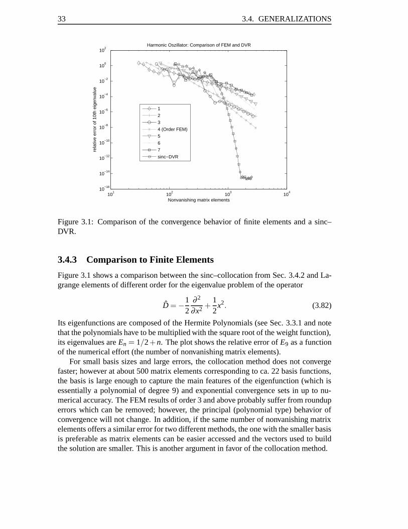
Figure 3.1: Comparison of the convergence behavior of finite elements and a sinc–DVR.
3.4.3 Comparison to Finite Elements
Figure 3.1 shows a comparison between the sinc–collocation from Sec. 3.4.2 and La-grange elements of different order for the eigenvalue problem of the operator
D = −12
∂ 2
∂x2 +12
x2. (3.82)
Its eigenfunctions are composed of the Hermite Polynomials (see Sec. 3.3.1 and notethat the polynomials have to be multiplied with the square root of the weight function),its eigenvalues are En = 1/2+n. The plot shows the relative error of E9 as a functionof the numerical effort (the number of nonvanishing matrix elements).
For small basis sizes and large errors, the collocation method does not convergefaster; however at about 500 matrix elements corresponding to ca. 22 basis functions,the basis is large enough to capture the main features of the eigenfunction (which isessentially a polynomial of degree 9) and exponential convergence sets in up to nu-merical accuracy. The FEM results of order 3 and above probably suffer from rounduperrors which can be removed; however, the principal (polynomial type) behavior ofconvergence will not change. In addition, if the same number of nonvanishing matrixelements offers a similar error for two different methods, the one with the smaller basisis preferable as matrix elements can be easier accessed and the vectors used to buildthe solution are smaller. This is another argument in favor of the collocation method.
CHAPTER 3. NUMERICAL METHODS 34
In the literature, an absolute accuracy of ≈ 10−9 has been reported for E9 whenusing 20 [65] and 28 [64] Lagrange elements of order eight, corresponding to about20 · 8 · 10 = 1600 and 28 · 8 · 10 = 2240 nonvanishing matrix elements; for the latter,a nonuniform grid was used. In the first case, also mean–square and maximum–normerrors of the eigenfunctions were computed to be of the order 10−6. For a productansatz, the FEM error is restricted to these figures while in a collocation basis the (true)eigenfunctions up to an arbitrary high precision can be used. Taking into account thatquadrature errors will induce spurious states at about 3/4 of the maximum eigenvalue[66], a collocation method can accurately represent the eigenfunction to the aboveproblem with ≈ 14 basis functions having 196 nonvanishing matrix elements only.
Of course, the global ansatz functions of spectral methods induce certain limita-tions. First, one is restricted to essentially rectangular geometries (“essentially” in-tends that in the collocation method, grid points in regions where the solution (nearly)vanishes can be omitted [53]; see Sec. 3.5). Second, boundary conditions are deter-mined by the orthogonal functions used to build the collocation basis so that varyingthe boundary values requires further effort. Especially, Gauss quadrature points neverlie on the boundary by theorem 3.3.2; to enforce a (Dirichlet) boundary conditionnot automatically satisfied by the basis, Gauss–Lobatto or Gauss–Radau quadratureschemes need to be used [47].
3.5 PODVR of the Schroedinger Equation
In view of the general background outlined in sections 3.2, 3.3 and 3.4, the potentialoptimized discrete variable representation (PODVR) of the Hamiltonian presented asa numerical recipe in [52] can be associated with its general background. Specifically,consider a Hamiltonian of the form
H =n
∑i=1
Di︸ ︷︷ ︸T
+V (x1, . . . ,xn) (3.83)
with T representing the kinetic energy operator in n degrees of freedom. Each Di is aderivative operator depending on one coordinate xi only and V (x1, . . . ,xn) a function(acting as a multiplicative operator) representing the potential energy of the configura-tion specified by x1, . . . ,xn. Finally, we would like to compute the lower spectrum ofthis operator (a fixed number of eigenfunctions or all eigenfunctions below a certainenergy, resp.). For that purpose, we use a product collocation basis of the form ofEq. (3.68); the individual collocation basis functions ψ Ni
ni are not derived from orthog-onal polynomials, but from a more general set of orthogonal functions as described inSec. 3.4.2. These, in turn, are chosen to be the Ni lowest eigenfunctions of a suitableone–dimensional symmetric operator for each degree of freedom. While the choiceof the kinetic energy part for these “reference Hamiltonians” is obvious, the potential
35 3.6. DIAGONALIZATION TECHNIQUES
energy part needs some consideration. A possibility that often works is to minimizethe potential energy V along all other coordinates,
V iref(x
i) := minx j, j �=i
V (x1, . . . ,xn). (3.84)
For each degree of freedom, we then diagonalize the reference Hamiltonian
ˆHiref(x
i) := Di +V iref(x
i), (3.85)
yielding Ni (orthogonal) eigenfunctions fi which, in a next step, are used in Eq. (3.71).The fi can in turn be conveniently computed by using the generic sinc–DVR, Eq. (3.80)and (3.81), for radial degrees of freedom and Legendre polynomials (see Eq. (3.53))for angular variables. The matrix elements of the fi with the position operator neededin Eq. (3.71) are then consistently evaluated in a quadrature approximation by repre-senting the position operator in the collocation basis as diagonal and transforming thisrepresentation to the basis of the fi functions.
In a last step, all product collocation basis functions are discarded for which thecorresponding collocation points (x1
i1, . . . ,xnin) satisfy
V (x1i1, . . . ,x
nin) > Vcut (3.86)
with a suitably chosen energy Vcut which can be considered infinite for the purposeof the calculation. This amounts to setting the wavefunction to zero at these points.Blocking of the vectors to use BLAS 3–routines (cf. Sec. 3.4.1) requires these pointsto be filled with zeros; nevertheless, storage requirements are less and the condition ofthe matrix will be improved.
3.6 Diagonalization Techniques
The choice of a proper method to diagonalize the matrix representation of the Hamil-tonian is another key issue for the efficiency of the entire algorithm. The appropri-ate class of diagonalization techniques consists in matrix–vector algorithms owing tothe sparsity of the (large) matrices. A standard program package for that purpose isARPACK [69].
In the first subsection, we discuss the error measure to be used in approximatematrix–vector algorithms. A measure different from the one used in the ARPACKpackage is proposed. The second subsection contains a summary of the algorithmused in the present calculations (Lanczos with Partial Reorthogonalization). The thirdbriefly summarizes another strategy (the Jacobi–Davidson method) and investigatesits criterion to determine the number of iteration steps. The fourth finally contains aproposal to better exploit the search subspaces build in the Jacobi–Davidson methodin order to obtain an efficient method for many eigenvalues.
CHAPTER 3. NUMERICAL METHODS 36
3.6.1 Error Measure
For any approximation x of an eigenvector x of a (symmetric) matrix H, the residual ris given by
r = Hx−θ x, (3.87)
where θ = (x,Hx) is a (Ritz) approximation for the true eigenvalue λ , Hx = λx (alleigenvectors and approximate eigenvectors assumed normalized). If a specific toler-ance ε is allowed for the approximation of x, the first idea is to compare ε to the norm||r|| of the residual. This measure, however, would not be scale invariant. ARPACKessentially uses the criterion
1θ||r|| ≤ ε (3.88)
which solves the problem of scale invariance. However, this measure still does notaccount properly for clustered eigenvalues. We thus propose
rλ :=1δ||r|| ≤ ε (3.89)
where δ := minj|θ − θ j| and the θ j summarize all other Ritz values. This criterion,
being both shift–and scale invariant, gives reliable error bounds on scalar products ofapproximate eigenvectors. To be more specific, we have the following error bound forthe eigenvector approximation x [70, 71, 72]:
sin(x, x) ≤ ||r||δe
(3.90)
with δe := minj|θ − λ j| and λ j being the exact eigenvalues. For the overlap matrix
elements of two eigenvectors x1,x2 in two adjacent sectors, this gives an error estimate
|(x1, x2)− (x1,x2)| <∼ 2rλ (3.91)
where the estimate would hold exactly if, on the one hand, x1 and x2 referred to thesame matrix (the difference of adjacent surface Hamiltonians is small, however). Onthe other hand, we would have to use δe instead of δ in the definition of rλ ; again, inpractice this will not cause problems: The Ritz values are close to the true eigenvaluesas they usually are better converged than the approximations for the eigenvectors.
Along the same line of argument, the non–orthogonality of two approximate eigen-vectors will also be bound by this quantity such that one can be sure of a certain levelof orthogonality without (re–)orthogonalization of all eigenvectors.
3.6.2 Lanczos with Partial Reorthogonalization
To obtain the first Nch eigenvalues and eigenstates used in the scattering calculations,we can exploit the sparsity of the resulting PODVR Hamiltonian matrix and implement
37 3.6. DIAGONALIZATION TECHNIQUES
a slight variation of the Lanczos algorithm [73] with partial reorthogonalization [74].The latter procedure in its original form has, for example, been already used by Yu andNyman [75] in quantum-chemical calculations.
By the well–known Lanczos recursion relation,
Hqk = βk−1qk−1 +αkqk +βkqk+1, (3.92)
with β0q0 = 0 and an initial vector q1 we generate a tridiagonal matrix representationTn = QT
n HQn, Qn = (q1, . . . ,qn) with orthonormal columns qk,
Tn =
⎛⎜⎜⎜⎜⎝
α1 β2 . . . 0
β2 α2. . .
.... . . . . . . . .
.... . . . . . βn
0 . . . βn αn
⎞⎟⎟⎟⎟⎠ . (3.93)
Tn is the orthogonal projection of the PODVR Hamiltonian matrix H onto the Krylovsubspace K (q1,H,n) = span{q1,Hq1, . . . ,H
nq1} with basis Qn. Evaluation of therecursion relation, Eq. (3.92), uses matrix–vector multiplications only, thus exploitingthe sparsity of H. The eigenvalues θk and eigenvectors sk of Tn can be determinedat low computational cost. If n equals the number of rows resp. columns of H, theeigenvalues are the same as those of H and the eigenvectors can be easily transformedto yield yk = Qnsk. For smaller n, we have an error bound
res(k) = ||Hyk −θkyk||2 = |βn||snk| (3.94)
where snk is the last component of the k-th eigenvector of Tn.The common problem of numerical non–orthogonality of the qk can be handled by
full reorthogonalization of each new qn against all previous ones. However, this com-putationally demanding procedure is unnecessary as non–orthogonality usually arisesfrom the convergence of an eigenvector (cf. Eq. (3.94) and (3.92)) which does not oc-cur in every Lanczos step. If n+1 steps are performed, partial reorthogonalization [74]estimates the orthogonality components in the (n+1)–th step, ωn+1,k = qT
n+1qk, by therecurrence relation
ωkk = 1, k = 1, . . . ,n,
ωk,k−1 = Ψk, k = 2, . . . ,n, (3.95)
ωn+1,k =1
βn+1
(βk+1ωn,k+1 +(αk −αn)ωnk +βkωn,k−1 −βnωn−1,k
)+ϑnk
for 1≤ k < n, with ωn0 = 0. Ψk and ϑnk are suitably chosen random numbers to accountfor the roundoff errors. This relation avoids to compute the scalar products qT
n+1qk inevery step.
Non–orthogonal vectors usually come in batches; we intend to keep semi–ortho-gonality at a level
√εmach where εmach is the machine precision. Reorthogonalization
CHAPTER 3. NUMERICAL METHODS 38
is performed for qn+1 if |ωn+1,k| ≥ √εmach against all neighboring qi, k − s < i <
k + r, where r and s are the smallest positive indices such that |ωn+1,k−s| < η and
|ωn+1,k+r| < η , with η being usually chosen as η = ε 3/4mach. If a batch has been found,
it is used in two consecutive Lanczos steps for reorthogonalization. After reorthogo-nalization, ωn+1,i is reset to a random value reflecting the regained orthogonality up toround-off level.
To our experience, Eq. (3.95) estimates the round-off errors quite well, but smallunderestimations which are randomly occurring might nevertheless destroy orthogo-nality at a certain point. We thus use the absolute values in the last line of Eq. (3.95),i.e.
ωn+1,k =1
βn+1
(|βk+1ωn,k+1|+ |(αk −αn)ωnk|+ |βkωn,k−1|+ |βnωn−1,k|
)+ |ϑnk|
(3.96)and replace ϑnk (proposed by Simon [74] as ϑnk = εmach(βk+1 + βn+1)Θ, where Θis normally distributed with mean 0 and standard deviation 0.3) by the non–randomquantity ϑnk = εmach(βk+1 + βn+1). (Note that βk > 0 for all k). ωn+1,n is evaluatedas scalar product instead of using a random number Ψn+1. While this formula largelyoverestimates the orthogonality components, no random underestimations will occurin our calculation that could destroy orthogonality. After orthogonalization of qn+1against qi, ωn+1,i is set to εmach.
It is reasonable to test for convergence of the first Nch eigenvectors in regular inter-vals, for example after each integer multiple of Nch. The iteration will then be stoppedat a step NLanczos = MrepNch if maxk=1,...,n res(k) ≤ rmax (this can be replaced by thecriterion (3.89)).
For the initial vector q1, we observe a slight increase in convergence speed whenit is computed as the normalized average of the first Nch eigenvectors of the previoussector instead of a randomly chosen vector. Overall, the performance is superior toARPACK due to the many eigenvectors computed such that contraction of the searchspace is unfavorable.
3.6.3 The Jacobi–Davidson Method
In the Jacobi–Davidson method [76], the Ritz approximation (x,θ ) to an eigenpair(x,λ ) is not obtained in a Krylov subspace, but in a more general search space Vn =span{v1, . . . ,vn}. The interesting property of this ansatz is that several starting vec-tors instead of just one can be provided so that the eigenvector information from theprevious sector does not have to be collapsed into a single vector. This is especiallyinteresting for the proper resolution of avoided crossings occurring in a small range ofthe reaction coordinate.
The space Vn is expanded by computing a Jacobi–Davidson update [77] to the Ritzapproximation x:
(I− xx∗)(H−θI)(I− xx∗)t = −r (3.97)
39 3.6. DIAGONALIZATION TECHNIQUES
where x∗ denotes transposition. x+ t is then a better approximation for x.Eq. (3.97), in turn, has to be solved by some approximate method; a possible choice
is MINRES [78]. In this algorithm, a Krylov subspace of size m is build up by theLanczos recursion and the correction equation is solved approximately in this space.The (maximum) iteration number mmax need not be guessed: The norm of the residualof x + t is composed of the norm ||r2|| of the residual resulting from the approximatesolution of (3.97) and an error contribution from the deviation of θ from the trueeigenvalue:
||H(x+ t)−θ(x+ t)||2 = (x,Ht)2 + ||r2||2. (3.98)
The Krylov subspace in MINRES can then be expanded as long as ||r2||2 domi-nates. Otherwise, it is better to restart with the optimized Ritz value obtained ei-ther directly from x + t or from rediagonalization of H in the extended subspaceVn+1 = span{v1, . . . ,vn, t}.
3.6.4 Combining Lanczos and Jacobi–Davidson
The drawback we experienced in using the Jacobi–Davidson method lies in the factthat for many eigenvectors to be computed, during the update of a single vector, theKrylov subspace of MINRES will also generate information about the other vectorswhich is lost once the correction equation (3.97) has been solved. In addition, thesubspace Vn and thus the matrix to be diagonalized might become very large.
A possible way to tackle these problems is to first replace x by x + t instead ofaugmenting Vn by t. Second, we can solve the correction equation for the othereigenvector approximations in the same Krylov subspace. More specifically, let ybe such an eigenvector approximation with Ritz value σ , residual s and assume Wm =span{w1, . . . ,wm} to be a reasonable part of this Krylov subspace (for example, com-posed of the m lowest eigenvectors of the tridiagonal matrix Tn, Eq. (3.93)), projectedonto the space orthogonal to y. In view of Eq. (3.98), we then need to find a solutionto
minw∈Wm
(||b−Hσ w||2 +(y,Hw)2) (3.99)
with Hσ = (I− yy∗)(H−σI)(I− yy∗) and b = −s. Writing
w =m
∑i=1
aiwi,
and setting the partial derivatives w.r.t the ai to zero, we obtain the matrix equation
Hreda = bred (3.100)
with
(Hred)i j = (Hσ wi,Hσ w j)+(y,Hwi)(y,Hw j) and (3.101)
(bred)i = (−s,Hσ wi). (3.102)
CHAPTER 3. NUMERICAL METHODS 40
We can rewrite Hred as
(Hred)i j =((H−σI)wi,(H−σI)w j
)(3.103)
showing the positive definiteness (unless σ is an exact eigenvalue) and thus the exis-tence of a local minimum. Solution of the (lower dimensional) equation (3.100) givesthe vector w which can then be used to update y as y+w.
The benefit of this procedure lies in the possibility of using several smaller sub-spaces instead of one large space, and this will decrease reorthogonalization effortwhich scales quadratically with the number of basis vectors. The Lanczos algorithmusually converges the eigenvalues at the outer parts of the spectrum first; therefore, re-peated construction of Krylov subspaces recomputes very similar information. We canof course orthogonalize against converged eigenvector approximations, but doing thisin every Lanczos step will introduce unnecessary overhead. In an exact calculation, itshould suffice to start with an orthogonalized vector q1: If the eigenvector approxima-tion x of x to be orthogonalized against were exact and if exact arithmetic were used,all consecutive Lanczos vectors would remain orthogonal to x. In practice, similar to(3.91), the scalar product of the initial vector q1 with x will be no larger than ε1 = rλif q1 is numerically orthogonal to x; and the analogous quantities εk for the vectors qkfulfill a recursion relation
βkεk+1 = (λ −αk)εk −βk−1εk−1 (3.104)
where λ is the exact eigenvalue corresponding to x. By monitoring the components ofthe qk in the directions of the converged eigenvectors in this way, we should have toreorthogonalize only when necessary.

Chapter 4
Results
The contents of the first three sections of this chapter have been published [79,82,83].For the sake of brevity, theoretical particularities and numerical details can be found inthe corresponding papers. Additional material concerning cross sections can be foundin [81] and kinetic isotope effects are studied in [80, 84].
4.1 Cl–Cl Exchange Reaction
4.1.1 Abstract
Time–independent quantum scattering calculations have been carried out on the Wal-den inversion SN2 reaction Cl− + CH3Cl′ (v1,v2,v3) → ClCH3 (v′1,v
′2,v
′3) + Cl′−. The
two C–Cl stretching modes (quantum numbers v3 and v′3) and the totally symmetricinternal modes of the methyl group (C–H stretching vibration, v1 and v′1, and inver-sion bending vibration, v2 and v′2) are treated explicitly. A four–dimensional coupledcluster potential energy surface is employed. The scattering problem is formulated inhyperspherical coordinates using the exact Hamiltonian and exploiting the full sym-metry of the problem. Converged state–selected reaction probabilities and productdistributions have been calculated up to ca. 6000 cm−1 above the vibrational groundstate of CH3Cl, i.e. up to initial vibrational excitation (2,0,0). In order to extract allscattering resonances, the energetic grid was chosen to be very fine, partly down toa resolution of 10−12 cm−1. Up to 2500 cm−1 translational energy, initial excitationof the umbrella bending vibration, (0,1,0), is more efficient for reaction then excitingthe C–Cl stretching mode, (0,0,1). The combined excitation of both vibrations resultsin a synergic effect, i.e. a considerably higher reaction probability than expected fromthe sum of both independent excitations, even higher than (0,0,2) up to 1500 cm−1
translational energy. Product distributions show that the umbrella mode is stronglycoupled to the C–Cl stretching mode and cannot be treated as a spectator mode. Thereaction probability rises almost linearly with increasing initial excitation of the um-brella bending mode. The effect with respect to the C–Cl stretch is five times larger for
CHAPTER 4. RESULTS 42
more than two quanta in this mode, and in agreement with previous work saturationis found. Exciting the high–frequency C–H stretching mode, (1,0,0), yields a largeincrease for small energies (more than two orders of magnitude larger than (0,0,0)),while for translational energies higher than 2000 cm−1, it becomes a pure spectatormode. For combined initial excitations including the symmetric C–H stretch, the spec-tator character of the latter is even more pronounced. However, up to more than 1500cm−1 translational energy, the C–H vibration does not behave adiabatically during thecourse of reaction because only 20 % of the initial energy is found in the same modein the product molecule. The distribution of resonance widths and peak heights is dis-cussed, and it is found that individual resonances pertinent to intermediate complexesCl− · · ·CH3Cl show product distributions independent of the initial vibrational state ofthe reactant molecule. The relatively high reactivity, with respect to excitation of anymode, of resonance states found in previous work is confirmed in the present calcula-tions. However, reactivity of intermediate states and reactivity with respect to initialvibrational excitation have to be distinguished. There is a strong mixing between thevibrational states reflected in numerous avoided crossings of the hyperspherical adia-batic curves.
4.1.2 Introduction
Clary and Palma [91] performed the first quantum scattering and additional classicaltrajectory calculations on the symmetric chlorine exchange SN2 reaction
Cl− +CH3Cl′ → ClCH3 +Cl′ (4.1)
including three internal degrees of freedom: the broken and the formed C–Cl bondsand the CH3 umbrella bending angle. The kinetic energy of the latter mode was ex-pressed in terms of an approximate operator with Legendre polynomials as eigenfunc-tions. These authors found that excitation of the inversion mode apparently does nothave a large influence on the reaction probability. These three–mode calculations wererepeated by Yu and Nyman [92] employing a different Hamiltonian that was based ontheir rotating line umbrella (RLU) method and was exact within the chosen 3D modelfor the reaction. Here, the umbrella mode was considered as a stretching–type mo-tion of the carbon atom against the three hydrogens with the other degrees of freedomoptimized. Yu and Nyman obtained a conclusion very similar to that of Clary andPalma.
In this work, the Hamiltonian developed for the filter–diagonalization calculationsof resonances states [94] is used in four–mode quantum scattering calculations on theWalden inversion reaction Cl−+CH3Cl′ →ClCH3 +Cl′. To our best knowledge, theseare the first four–dimensional (4D) time–independent quantum scattering calculationson a complex–forming bimolecular reaction. They require a high energy resolutionand are thus very CPU-intensive.
For an exact description of the Cl− + CH3Cl′ SN2 system, twelve degrees of free-dom have to be taken into account explicitly so that a rigorous state–selective quantum
43 4.1. CL–CL EXCHANGE REACTION
mechanical treatment appears to be impossible at present. Furthermore, if the rota-tional motion of the whole system were included, the three Euler angles would haveto be considered additionally. We thus reduce the dimensionality of the Cl− + CH3Cl′→ ClCH3 + Cl′− reaction and study the system under the restriction that C3v sym-metry is maintained throughout the reactive process. Since the minimum energy pathpertinent to the Walden inversion reaction is collinear and the potential energy rises inall directions perpendicular to the minimum energy path, we adopt a model that ex-plicitly takes into account the two carbon–chlorine distances and the totally symmetriccoordinates of the methyl group (corresponding to umbrella bending and symmetricC–H stretching vibrations). As was described in Ref. [94], the motion of the atomsunder the restriction of C3v symmetry (for total angular momentum J = 0) can be de-scribed exactly, i.e., without any further dynamical approximation. However, evenin this symmetry–restricted dimensionality–reduced model, the present SN2 system iscomputationally rather demanding because the clusters exhibit low intermolecular fre-quencies in conjunction with far–reaching ion–dipole potentials. Time–independentquantum scattering calculations in four dimensions have been reported for the reactionO (3P) + CH4 → OH + CH3 by Palma and Clary [85, 86] and Yu and Nyman [87].However, in this reaction not the methyl group but only a hydrogen atom is trans-ferred and resonances do not play any role because intermediate complexes betweenthe open-shell atom and the spherical top methane are not formed. Palma and Clarystudied the influence of excitation of umbrella bending and symmetric and antisym-metric C–H stretching modes on the reaction probability and found that all modespromote the reaction. While this effect is evident for O + CH4 because one C–H bondis broken and both symmetric and antisymmetric C–H stretch in CH4 affect this bond,the nature of the C–H stretch in an SN2 process is entirely different: it does not changeduring the course of reaction and thus a spectator–like behavior is expected.
Experiments on the detailed, state–selective dynamics of gas–phase SN2 reactionsare scarce. Ervin and co–workers studied the promotion of the Cl− + CH3Cl′ → ClCH3+ Cl′ reaction by kinetic energy via guided ion beam tandem mass spectrometry [14].Bierbaum and coworkers [10] could determine the thermal rate coefficient at 300 K tobe k = (3.5±1.8)×10−14 cm3 s−1.
4.1.3 Results
Potential and Surface Eigenstates
Plots along the hyperangle δ with z and q optimized are shown in Fig. 4.1. The cut forρ = 10 a0 has a local maximum in the saddle point region of the PES. For very largevalues of ρ , two deep wells corresponding to reactants and products are separated by abroad and high potential barrier. Due to the symmetry of the potential, the wavefunc-tions are either symmetric (gerade) or antisymmetric (ungerade) with respect to 1
2δmax.In order to localize the wavefunctions in either of the asymptotic channels, appropriatelinear combinations of gerade and ungerade wavefunctions are formed. Note that the
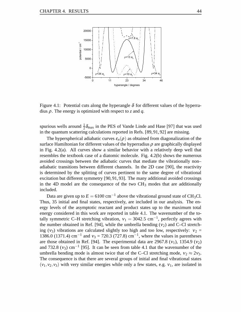
CHAPTER 4. RESULTS 44
ρ
ρ
ρ
ρ ρ
Figure 4.1: Potential cuts along the hyperangle δ for different values of the hyperra-dius ρ . The energy is optimized with respect to z and q.
spurious wells around 12δmax in the PES of Vande Linde and Hase [97] that was used
in the quantum scattering calculations reported in Refs. [89, 91, 92] are missing.The hyperspherical adiabatic curves εn(ρ) as obtained from diagonalization of the
surface Hamiltonian for different values of the hyperradius ρ are graphically displayedin Fig. 4.2(a). All curves show a similar behavior with a relatively deep well thatresembles the textbook case of a diatomic molecule. Fig. 4.2(b) shows the numerousavoided crossings between the adiabatic curves that mediate the vibrationally non–adiabatic transitions between different channels. In the 2D case [90], the reactivityis determined by the splitting of curves pertinent to the same degree of vibrationalexcitation but different symmetry [90, 91, 93]. The many additional avoided crossingsin the 4D model are the consequence of the two CH3 modes that are additionallyincluded.
Data are given up to E = 6100 cm−1 above the vibrational ground state of CH3Cl.Thus, 35 initial and final states, respectively, are included in our analysis. The en-ergy levels of the asymptotic reactant and product states up to the maximum totalenergy considered in this work are reported in table 4.1. The wavenumber of the to-tally symmetric C–H stretching vibration, ν1 = 3042.5 cm−1, perfectly agrees withthe number obtained in Ref. [94], while the umbrella bending (ν2) and C–Cl stretch-ing (ν3) vibrations are calculated slightly too high and too low, respectively: ν2 =1386.0 (1371.4) cm−1 and ν3 = 720.3 (727.8) cm−1, where the values in parenthesesare those obtained in Ref. [94]. The experimental data are 2967.8 (ν1), 1354.9 (ν2)and 732.8 (ν3) cm−1 [95]. It can be seen from table 4.1 that the wavenumber of theumbrella bending mode is almost twice that of the C–Cl stretching mode, ν2 ≈ 2ν3.The consequence is that there are several groups of initial and final vibrational states(v1,v2,v3) with very similar energies while only a few states, e.g. ν1, are isolated in
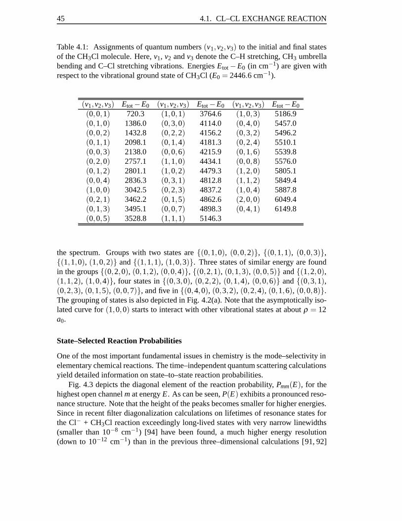
45 4.1. CL–CL EXCHANGE REACTION
Table 4.1: Assignments of quantum numbers (v1,v2,v3) to the initial and final statesof the CH3Cl molecule. Here, v1, v2 and v3 denote the C–H stretching, CH3 umbrellabending and C–Cl stretching vibrations. Energies Etot −E0 (in cm−1) are given withrespect to the vibrational ground state of CH3Cl (E0 = 2446.6 cm−1).
(v1,v2,v3) Etot −E0 (v1,v2,v3) Etot −E0 (v1,v2,v3) Etot −E0
(0,0,1) 720.3 (1,0,1) 3764.6 (1,0,3) 5186.9(0,1,0) 1386.0 (0,3,0) 4114.0 (0,4,0) 5457.0(0,0,2) 1432.8 (0,2,2) 4156.2 (0,3,2) 5496.2(0,1,1) 2098.1 (0,1,4) 4181.3 (0,2,4) 5510.1(0,0,3) 2138.0 (0,0,6) 4215.9 (0,1,6) 5539.8(0,2,0) 2757.1 (1,1,0) 4434.1 (0,0,8) 5576.0(0,1,2) 2801.1 (1,0,2) 4479.3 (1,2,0) 5805.1(0,0,4) 2836.3 (0,3,1) 4812.8 (1,1,2) 5849.4(1,0,0) 3042.5 (0,2,3) 4837.2 (1,0,4) 5887.8(0,2,1) 3462.2 (0,1,5) 4862.6 (2,0,0) 6049.4(0,1,3) 3495.1 (0,0,7) 4898.3 (0,4,1) 6149.8(0,0,5) 3528.8 (1,1,1) 5146.3
the spectrum. Groups with two states are {(0,1,0), (0,0,2)}, {(0,1,1), (0,0,3)},{(1,1,0), (1,0,2)} and {(1,1,1), (1,0,3)}. Three states of similar energy are foundin the groups {(0,2,0), (0,1,2), (0,0,4)}, {(0,2,1), (0,1,3), (0,0,5)} and {(1,2,0),(1,1,2), (1,0,4)}, four states in {(0,3,0), (0,2,2), (0,1,4), (0,0,6)} and {(0,3,1),(0,2,3), (0,1,5), (0,0,7)}, and five in {(0,4,0), (0,3,2), (0,2,4), (0,1,6), (0,0,8)}.The grouping of states is also depicted in Fig. 4.2(a). Note that the asymptotically iso-lated curve for (1,0,0) starts to interact with other vibrational states at about ρ = 12a0.
State–Selected Reaction Probabilities
One of the most important fundamental issues in chemistry is the mode–selectivity inelementary chemical reactions. The time–independent quantum scattering calculationsyield detailed information on state–to–state reaction probabilities.
Fig. 4.3 depicts the diagonal element of the reaction probability, Pmm(E), for thehighest open channel m at energy E. As can be seen, P(E) exhibits a pronounced reso-nance structure. Note that the height of the peaks becomes smaller for higher energies.Since in recent filter diagonalization calculations on lifetimes of resonance states forthe Cl− + CH3Cl reaction exceedingly long-lived states with very narrow linewidths(smaller than 10−8 cm−1) [94] have been found, a much higher energy resolution(down to 10−12 cm−1) than in the previous three–dimensional calculations [91, 92]
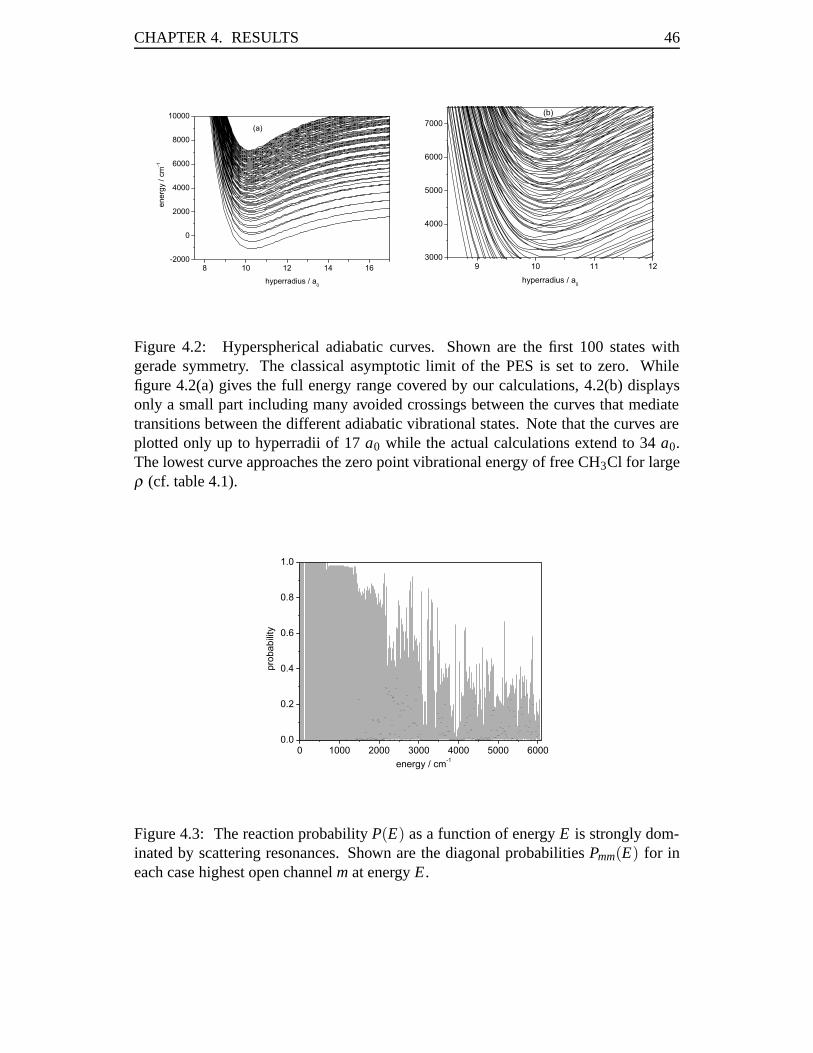
CHAPTER 4. RESULTS 46
Figure 4.2: Hyperspherical adiabatic curves. Shown are the first 100 states withgerade symmetry. The classical asymptotic limit of the PES is set to zero. Whilefigure 4.2(a) gives the full energy range covered by our calculations, 4.2(b) displaysonly a small part including many avoided crossings between the curves that mediatetransitions between the different adiabatic vibrational states. Note that the curves areplotted only up to hyperradii of 17 a0 while the actual calculations extend to 34 a0.The lowest curve approaches the zero point vibrational energy of free CH3Cl for largeρ (cf. table 4.1).
Figure 4.3: The reaction probability P(E) as a function of energy E is strongly dom-inated by scattering resonances. Shown are the diagonal probabilities Pmm(E) for ineach case highest open channel m at energy E.

47 4.1. CL–CL EXCHANGE REACTION
Figure 4.4: Initial state–selected reaction probabilities Pm(E) for Cl− + CH3Cl′(v1,v2,v3)→ ClCH3 + Cl′− as functions of translational energy Etrans. The data issmoothed over intervals of 80 cm−1. Pmn(E) is summed over all accessible productchannels n. The dashed curves belong to initial excitation with one quantum in thehigh–frequency C–H stretching vibration.
was used in order to detect all resonances. In order to be able to quantitatively com-pare the influence of different initial vibrational excitations in the reactant molecules,in the following the strongly fluctuating probabilities were averaged over intervals ofΔ = 80 cm−1, i.e. each point P(E) is the average of the probability in the energeticrange [E − 1
2Δ, E + 12Δ].
The initial state–selected reaction probabilities Pm(E), summed over all productstates,
Pm(E) = ∑n
Pmn(E) = ∑n|Smn(E)|2 (4.2)
as functions of translational energy Etrans are graphically displayed in Figs. 4.4 and4.5. Since the curves are not shown as functions of total energy, their energetic range isdifferent. To obtain the probabilities as functions of Etot, shift the energetic scale by therespective level energies given in table 4.1. As anticipated from the two–dimensionalresults [96], the reaction probability increases with excitation of the intramolecularC–Cl stretching mode ν3.
As seen from Fig. 4.4, the probability with initial excitation (0,0,0) rises withsome fluctuations continuously and exponentially. When the C–Cl stretching modeis excited by one quantum, P(E) becomes larger by 2–3 orders of magnitude. Forsmall translational energies, the reaction probability for initial excitation (0,0,2) is
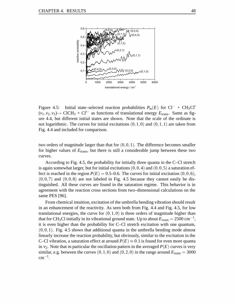
CHAPTER 4. RESULTS 48
Figure 4.5: Initial state–selected reaction probabilities Pm(E) for Cl− + CH3Cl′(v1,v2,v3)→ ClCH3 + Cl′− as functions of translational energy Etrans. Same as fig-ure 4.4, but different initial states are shown. Note that the scale of the ordinate isnot logarithmic. The curves for initial excitations (0,1,0) and (0,1,1) are taken fromFig. 4.4 and included for comparison.
two orders of magnitude larger than that for (0,0,1). The difference becomes smallerfor higher values of Etrans, but there is still a considerable jump between these twocurves.
According to Fig. 4.5, the probability for initially three quanta in the C–Cl stretchis again somewhat larger, but for initial excitations (0,0,4) and (0,0,5) a saturation ef-fect is reached in the region P(E) = 0.5–0.6. The curves for initial excitation (0,0,6),(0,0,7) and (0,0,8) are not labeled in Fig. 4.5 because they cannot easily be dis-tinguished. All these curves are found in the saturation regime. This behavior is inagreement with the reaction cross sections from two–dimensional calculations on thesame PES [96].
From chemical intuition, excitation of the umbrella bending vibration should resultin an enhancement of the reactivity. As seen both from Fig. 4.4 and Fig. 4.5, for lowtranslational energies, the curve for (0,1,0) is three orders of magnitude higher thanthat for CH3Cl initially in its vibrational ground state. Up to about E trans = 2500 cm−1,it is even higher than the probability for C–Cl stretch excitation with one quantum,(0,0,1). Fig. 4.5 shows that additional quanta in the umbrella bending mode almostlinearly increase the reaction probability, but obviously, similar to the excitation in theC–Cl vibration, a saturation effect at around P(E)≈ 0.1 is found for even more quantain ν2. Note that in particular the oscillation pattern in the averaged P(E) curves is verysimilar, e.g. between the curves (0,1,0) and (0,2,0) in the range around Etrans = 3000cm−1.
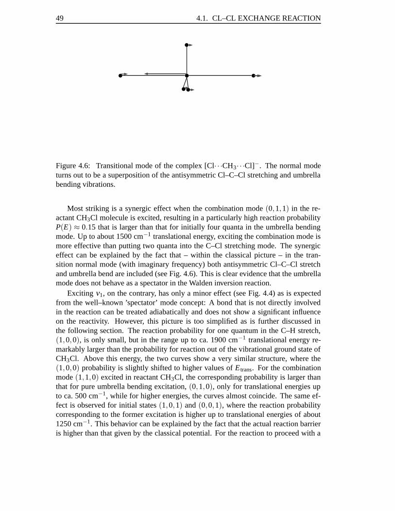
49 4.1. CL–CL EXCHANGE REACTION
Figure 4.6: Transitional mode of the complex [Cl· · ·CH3· · ·Cl]−. The normal modeturns out to be a superposition of the antisymmetric Cl–C–Cl stretching and umbrellabending vibrations.
Most striking is a synergic effect when the combination mode (0,1,1) in the re-actant CH3Cl molecule is excited, resulting in a particularly high reaction probabilityP(E) ≈ 0.15 that is larger than that for initially four quanta in the umbrella bendingmode. Up to about 1500 cm−1 translational energy, exciting the combination mode ismore effective than putting two quanta into the C–Cl stretching mode. The synergiceffect can be explained by the fact that – within the classical picture – in the tran-sition normal mode (with imaginary frequency) both antisymmetric Cl–C–Cl stretchand umbrella bend are included (see Fig. 4.6). This is clear evidence that the umbrellamode does not behave as a spectator in the Walden inversion reaction.
Exciting ν1, on the contrary, has only a minor effect (see Fig. 4.4) as is expectedfrom the well–known ’spectator’ mode concept: A bond that is not directly involvedin the reaction can be treated adiabatically and does not show a significant influenceon the reactivity. However, this picture is too simplified as is further discussed inthe following section. The reaction probability for one quantum in the C–H stretch,(1,0,0), is only small, but in the range up to ca. 1900 cm−1 translational energy re-markably larger than the probability for reaction out of the vibrational ground state ofCH3Cl. Above this energy, the two curves show a very similar structure, where the(1,0,0) probability is slightly shifted to higher values of E trans. For the combinationmode (1,1,0) excited in reactant CH3Cl, the corresponding probability is larger thanthat for pure umbrella bending excitation, (0,1,0), only for translational energies upto ca. 500 cm−1, while for higher energies, the curves almost coincide. The same ef-fect is observed for initial states (1,0,1) and (0,0,1), where the reaction probabilitycorresponding to the former excitation is higher up to translational energies of about1250 cm−1. This behavior can be explained by the fact that the actual reaction barrieris higher than that given by the classical potential. For the reaction to proceed with a
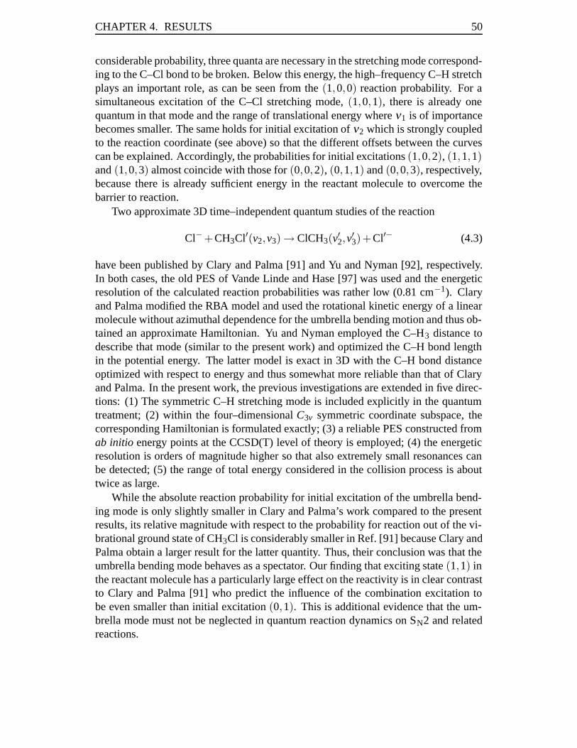
CHAPTER 4. RESULTS 50
considerable probability, three quanta are necessary in the stretching mode correspond-ing to the C–Cl bond to be broken. Below this energy, the high–frequency C–H stretchplays an important role, as can be seen from the (1,0,0) reaction probability. For asimultaneous excitation of the C–Cl stretching mode, (1,0,1), there is already onequantum in that mode and the range of translational energy where ν1 is of importancebecomes smaller. The same holds for initial excitation of ν2 which is strongly coupledto the reaction coordinate (see above) so that the different offsets between the curvescan be explained. Accordingly, the probabilities for initial excitations (1,0,2), (1,1,1)and (1,0,3) almost coincide with those for (0,0,2), (0,1,1) and (0,0,3), respectively,because there is already sufficient energy in the reactant molecule to overcome thebarrier to reaction.
Two approximate 3D time–independent quantum studies of the reaction
Cl− +CH3Cl′(v2,v3) → ClCH3(v′2,v′3)+Cl′− (4.3)
have been published by Clary and Palma [91] and Yu and Nyman [92], respectively.In both cases, the old PES of Vande Linde and Hase [97] was used and the energeticresolution of the calculated reaction probabilities was rather low (0.81 cm−1). Claryand Palma modified the RBA model and used the rotational kinetic energy of a linearmolecule without azimuthal dependence for the umbrella bending motion and thus ob-tained an approximate Hamiltonian. Yu and Nyman employed the C–H3 distance todescribe that mode (similar to the present work) and optimized the C–H bond lengthin the potential energy. The latter model is exact in 3D with the C–H bond distanceoptimized with respect to energy and thus somewhat more reliable than that of Claryand Palma. In the present work, the previous investigations are extended in five direc-tions: (1) The symmetric C–H stretching mode is included explicitly in the quantumtreatment; (2) within the four–dimensional C3v symmetric coordinate subspace, thecorresponding Hamiltonian is formulated exactly; (3) a reliable PES constructed fromab initio energy points at the CCSD(T) level of theory is employed; (4) the energeticresolution is orders of magnitude higher so that also extremely small resonances canbe detected; (5) the range of total energy considered in the collision process is abouttwice as large.
While the absolute reaction probability for initial excitation of the umbrella bend-ing mode is only slightly smaller in Clary and Palma’s work compared to the presentresults, its relative magnitude with respect to the probability for reaction out of the vi-brational ground state of CH3Cl is considerably smaller in Ref. [91] because Clary andPalma obtain a larger result for the latter quantity. Thus, their conclusion was that theumbrella bending mode behaves as a spectator. Our finding that exciting state (1,1) inthe reactant molecule has a particularly large effect on the reactivity is in clear contrastto Clary and Palma [91] who predict the influence of the combination excitation tobe even smaller than initial excitation (0,1). This is additional evidence that the um-brella mode must not be neglected in quantum reaction dynamics on SN2 and relatedreactions.
51 4.1. CL–CL EXCHANGE REACTION
Yu and Nyman1 cover translational energies for initial excitation (0,0) up to ca.3200 cm−1 and correspondingly smaller ranges for (0,1) and (1,0). The reactionprobability for initial excitation of the umbrella bending mode rises from 0.1 to 0.2at Etrans = 1600 cm−1, in good agreement with the results of the present work. Theprobability for (0,0) is slightly larger than that of the present work, while that for (0,1)is considerably increased. The present results show that in the energetic regime of Yuand Nyman’s work, the reaction probability for initial excitation (0,1) is throughoutbelow that for (1,0), while Yu and Nyman, on the contrary, obtain the reverse result forEtrans > 700 cm−1. Results on the effect of a combined excitation of ν2 and ν3 on thereactivity of the SN2 reaction are not reported by Yu and Nyman. Since their Hamil-tonian was exact within their 3D model, the differences to the reaction probabilitiesfrom the present work are mainly due to the disparate potential energy surfaces.
Product Distributions
If state–to–state reaction probabilities are normalized, Pmn(E)/Pm(E), product distri-butions are obtained. They are equivalent to relative probabilities with respect to aparticular initial state. Absolute state–to–state reaction probabilities can be recoveredby multiplying the summed absolute values in Figs. 4.4 and 4.5 with the percentageamounts of the product distributions.
Product distributions for the Cl− + CH3Cl′ (v1,v2,v3) → ClCH3Cl (v′1,v′2,v
′3) +
Cl′− reaction are graphically displayed in Figs. 4.7–4.11. Only the most importantproduct channels are shown, the curves corresponding to channels which are populatedonly to a very minor extent are not shown in the figures.
From Fig. 4.7, it is obvious that the reaction out of the vibrational ground stateof CH3Cl is most likely to end in product states with a high degree of vibrationalexcitation in the C–Cl stretching mode. Of course, for low translational energies, theonly open channel is (0,0,0). When a new channel with pure excitation in ν3 opensup, it becomes dominating in the product distribution until the next one opens (up tov3 = 4). However, for Etrans larger than 4000 cm−1, the product states (0,0,1) and(0,0,2) become most important. Also, the umbrella mode, (0,1,0), and the combinedexcitation (0,1,1) exhibit significant values in the product distribution.
Inspecting the product distributions for initial vibrational states (0,0, i), i = 1,2,3(Fig. 4.8), a similar behavior is observed, in particular for initially one quantum inthe C–Cl stretching vibration; for high Etrans, product excitations (0,0,1) and (0,0,2)dominate, while all other product vibrational states have only small probabilities.Thus, the transfer from vibrational energy (V) into translational energy (T) is onlyweak. For initial state (0,0,2), reaction in the equivalent product state is most likely,but also final state (0,0,3) is important for Etrans between 700 and 3000 cm−1. Forhigher translational energies, it is most likely to find the same number of quanta in
1Note that in their work, Yu and Nyman use the convention (v 3,v2) instead of the spectroscopicallymotivated nomenclature (v2,v3).
CHAPTER 4. RESULTS 52
Figure 4.7: Product distribution for Cl− + CH3Cl′ (0,0,0) → ClCH3 (v′1,v′2,v
′3) +
Cl′− for CH3Cl being initially in its vibrational ground state. The data is smoothedover intervals of 80 cm−1.
ν3 in reactant and product CH3Cl. Note that also product states with excitation of theumbrella bending mode play an important role, indicating the active role of this modein the reaction. For initial excitation (0,0,3), a similar effect can be seen. The sameproduct state as in the reactant molecule dominates up to 3000 cm−1. Also, the near–resonant mode (0,1,1) has a significant role, as well as the neighboring states (0,0,2)and (0,0,4) and the combined excitation (0,1,2). Again, V → T energy transfer is notobserved.
As can be seen from Fig. 4.9, exciting the umbrella bending mode in reactantCH3Cl favors products in the near–resonant state (0,0,2) while the state (0,1,0) isimportant only for low translational energies and shows a low population indicatingthat ν2 is not to be considered as a spectator mode. Also the states (0,0,3), and to aminor extent, (0,0,1) and (0,0,4) are populated in the product molecule. Furthermore,the combined excitations (0,1,1) and (0,1,2) are found in the product, indicating astrong tendency for T → V energy transfer when the umbrella mode is initially excited.Analogously, two quanta in the umbrella bending mode yield the product most likelyin the state (0,0,4), but also in the neighboring states (0,0,3) and (0,0,5). The near–resonant product state (0,1,2) is particularly important; its contribution drops from40 to 5% at 1500 cm−1 and then slowly rises again. The percentage of product state(0,2,1) is also remarkable, confirming the tendency to T → V energy transfer. Threeor four quanta in ν2 yield preferably a product with a high degree of excitation in theC–Cl mode, viz. (0,0,6) and (0,0,8), respectively. Initially v2 = 3 populates also thenear–resonant product states (0,1,4) and (0,2,2) as well as (0,0,7) and (0,3,1) whilev2 = 4 prefers the near–resonant states (0,1,6), (0,2,4) and (0,3,2) and a state with

53 4.1. CL–CL EXCHANGE REACTION
Figure 4.8: Product distribution for Cl− + CH3Cl′ (0,0, i)→ ClCH3 (v′1,v′2,v
′3) + Cl′−
with the C–Cl stretching vibration in CH3Cl initially excited with i = 1, 2, or 3 quanta,respectively. The data is smoothed over intervals of 80 cm−1.
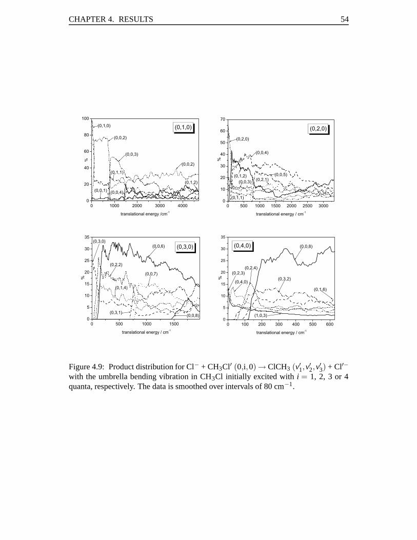
CHAPTER 4. RESULTS 54
Figure 4.9: Product distribution for Cl− + CH3Cl′ (0,i,0)→ ClCH3 (v′1,v′2,v
′3) + Cl′−
with the umbrella bending vibration in CH3Cl initially excited with i = 1, 2, 3 or 4quanta, respectively. The data is smoothed over intervals of 80 cm−1.
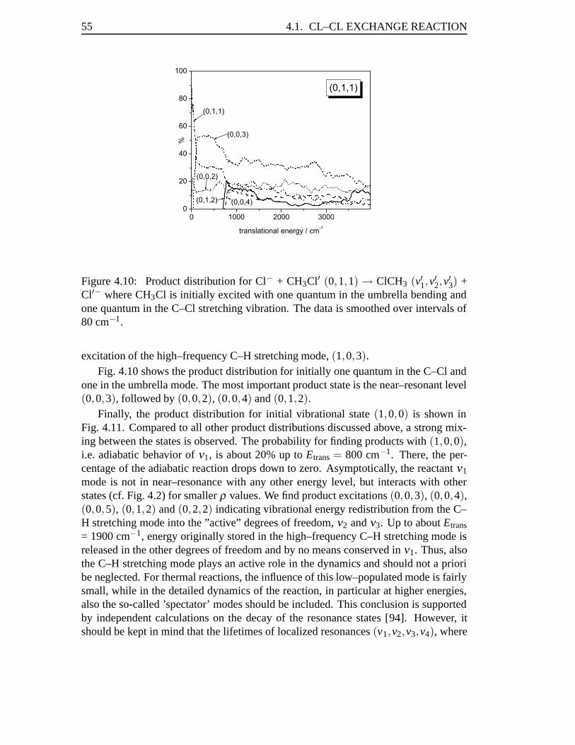
55 4.1. CL–CL EXCHANGE REACTION
Figure 4.10: Product distribution for Cl− + CH3Cl′ (0,1,1) → ClCH3 (v′1,v′2,v
′3) +
Cl′− where CH3Cl is initially excited with one quantum in the umbrella bending andone quantum in the C–Cl stretching vibration. The data is smoothed over intervals of80 cm−1.
excitation of the high–frequency C–H stretching mode, (1,0,3).Fig. 4.10 shows the product distribution for initially one quantum in the C–Cl and
one in the umbrella mode. The most important product state is the near–resonant level(0,0,3), followed by (0,0,2), (0,0,4) and (0,1,2).
Finally, the product distribution for initial vibrational state (1,0,0) is shown inFig. 4.11. Compared to all other product distributions discussed above, a strong mix-ing between the states is observed. The probability for finding products with (1,0,0),i.e. adiabatic behavior of ν1, is about 20% up to Etrans = 800 cm−1. There, the per-centage of the adiabatic reaction drops down to zero. Asymptotically, the reactant ν1
mode is not in near–resonance with any other energy level, but interacts with otherstates (cf. Fig. 4.2) for smaller ρ values. We find product excitations (0,0,3), (0,0,4),(0,0,5), (0,1,2) and (0,2,2) indicating vibrational energy redistribution from the C–H stretching mode into the ”active” degrees of freedom, ν2 and ν3. Up to about Etrans
= 1900 cm−1, energy originally stored in the high–frequency C–H stretching mode isreleased in the other degrees of freedom and by no means conserved in ν1. Thus, alsothe C–H stretching mode plays an active role in the dynamics and should not a prioribe neglected. For thermal reactions, the influence of this low–populated mode is fairlysmall, while in the detailed dynamics of the reaction, in particular at higher energies,also the so-called ’spectator’ modes should be included. This conclusion is supportedby independent calculations on the decay of the resonance states [94]. However, itshould be kept in mind that the lifetimes of localized resonances (v1,v2,v3,v4), where
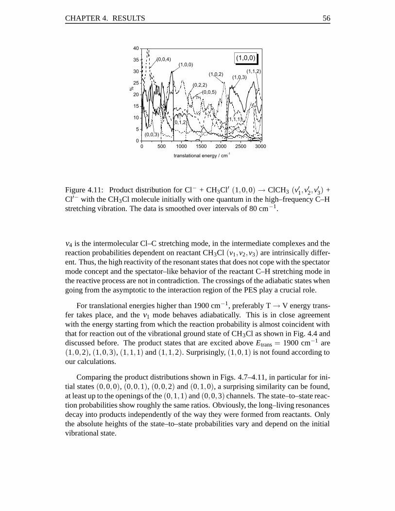
CHAPTER 4. RESULTS 56
Figure 4.11: Product distribution for Cl− + CH3Cl′ (1,0,0) → ClCH3 (v′1,v′2,v
′3) +
Cl′− with the CH3Cl molecule initially with one quantum in the high–frequency C–Hstretching vibration. The data is smoothed over intervals of 80 cm−1.
ν4 is the intermolecular Cl–C stretching mode, in the intermediate complexes and thereaction probabilities dependent on reactant CH3Cl (v1,v2,v3) are intrinsically differ-ent. Thus, the high reactivity of the resonant states that does not cope with the spectatormode concept and the spectator–like behavior of the reactant C–H stretching mode inthe reactive process are not in contradiction. The crossings of the adiabatic states whengoing from the asymptotic to the interaction region of the PES play a crucial role.
For translational energies higher than 1900 cm−1, preferably T → V energy trans-fer takes place, and the ν1 mode behaves adiabatically. This is in close agreementwith the energy starting from which the reaction probability is almost coincident withthat for reaction out of the vibrational ground state of CH3Cl as shown in Fig. 4.4 anddiscussed before. The product states that are excited above Etrans = 1900 cm−1 are(1,0,2), (1,0,3), (1,1,1) and (1,1,2). Surprisingly, (1,0,1) is not found according toour calculations.
Comparing the product distributions shown in Figs. 4.7–4.11, in particular for ini-tial states (0,0,0), (0,0,1), (0,0,2) and (0,1,0), a surprising similarity can be found,at least up to the openings of the (0,1,1) and (0,0,3) channels. The state–to–state reac-tion probabilities show roughly the same ratios. Obviously, the long–living resonancesdecay into products independently of the way they were formed from reactants. Onlythe absolute heights of the state–to–state probabilities vary and depend on the initialvibrational state.
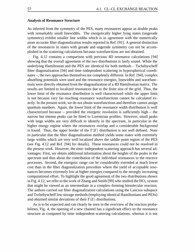
57 4.1. CL–CL EXCHANGE REACTION
Analysis of Resonance Structure
As inferred from the symmetry of the PES, many resonances appear as double peakswith remarkably small linewidths. The energetically higher lying states (ungeradesymmetry) exhibit smaller line widths which is in agreement with the numericallymore accurate filter diagonalization results reported in Ref. [91]. A general distinctionof the resonances in states with gerade and ungerade symmetry can not be accom-plished in the scattering calculations because wavefunctions are not obtained.
Fig. 4.12 contains a comparison with previous 4D resonance calculations [94]showing that the overall agreement of the two distributions is fairly sound. While theunderlying Hamiltonian and the PES are identical for both methods – Tschebyschefffilter diagonalization [94] and time–independent scattering in hyperspherical coordi-nates –, the two approaches themselves are completely different. In Ref. [94], complexabsorbing potentials were used and the resonance energies, linewidths and wavefunc-tions were directly obtained from the diagonalization of a 4D Hamiltonian matrix. Theresults are limited to localized resonances due to the finite size of the grid. Thus, thelower limit of the resonance distribution is well characterized while the upper limitis not because very far–reaching resonance wavefunctions cannot be calculated ex-actly. In the present work, we do not obtain wavefunctions and therefore cannot assignquantum numbers. Again, the lower limit of the resonance width distribution is wellcharacterized because – provided the energetic resolution is sufficiently high – thenarrow but intense peaks can be fitted to Lorentzian profiles. However, small peakswith large widths are very difficult to identify in the spectrum, in particular in thehigher energy regime where the resonances overlap and a considerable backgroundis found. Thus, the upper border of the Γ(E) distribution is not well defined. Notein particular that the filter diagonalization method yields some states with extremelylarge widths which are very well localized above the saddle point region of the PES(see Fig. 4.12 and Ref. [94] for details). These resonances could not be resolved inthe present work. However, the time–independent scattering approach has several ad-vantages: First, we obtain additional information about the heights of the peaks in thespectrum and thus about the contribution of the individual resonances to the reactiveprocesses. Second, the energetic range can be considerably extended at much lowercost than in the filter diagonalization procedure where the yield of acceptable reso-nances becomes extremely low at higher energies compared to the strongly increasingcomputational effort. To highlight the good agreement of the two distributions shownin Fig. 4.12, we refer to the work of Zhang and Smith [99] who studied the HO2 systemthat might be viewed as an intermediate in a complex–forming bimolecular reaction.The authors carried out filter diagonalization calculations using the Lanczos subspaceand Tschebyscheff low storage methods (employing identical Hamiltonians and PESs)and obtained similar deviations of their Γ(E) distributions.
As is to be expected and can clearly be seen in the overview of the reaction proba-bilities, Fig. 4, the opening of a new channel has a significant effect on the resonancestructure as computed by time–independent scattering calculations, whereas it is not
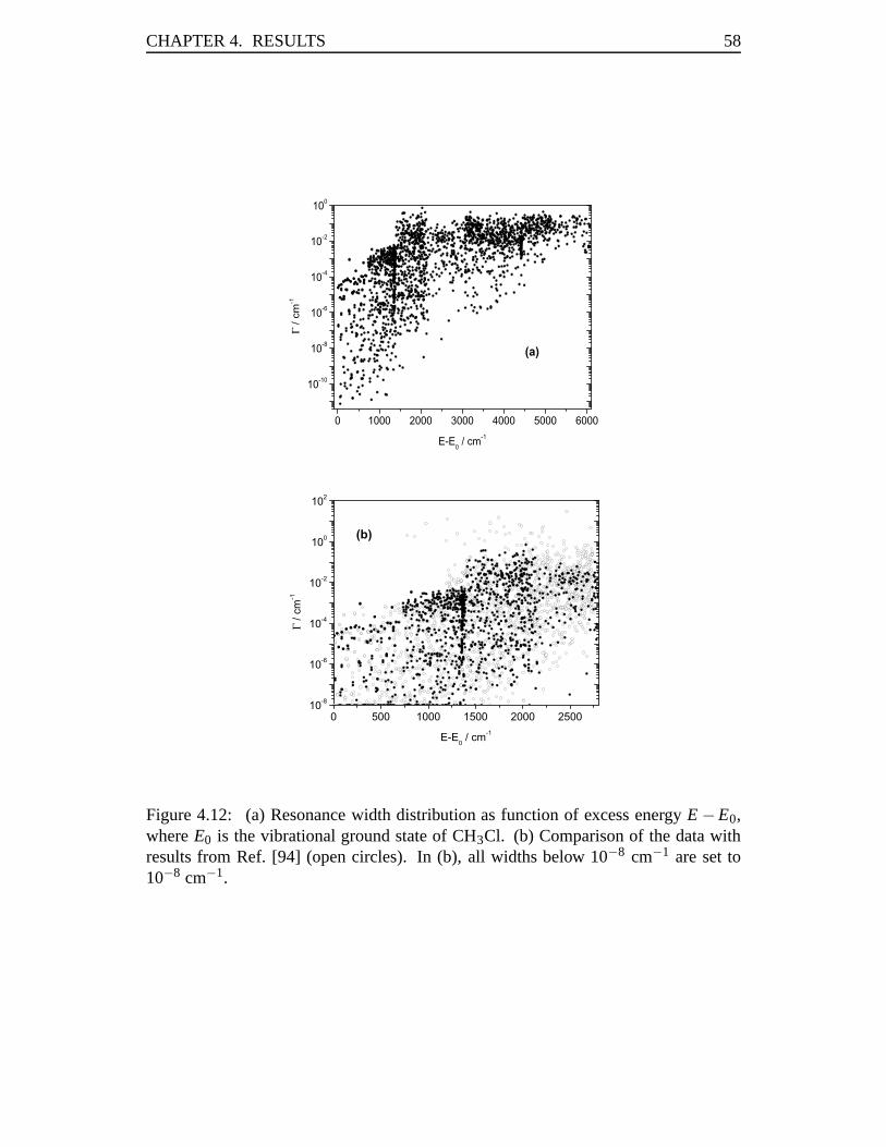
CHAPTER 4. RESULTS 58
ΓΓ
Figure 4.12: (a) Resonance width distribution as function of excess energy E −E0,where E0 is the vibrational ground state of CH3Cl. (b) Comparison of the data withresults from Ref. [94] (open circles). In (b), all widths below 10−8 cm−1 are set to10−8 cm−1.
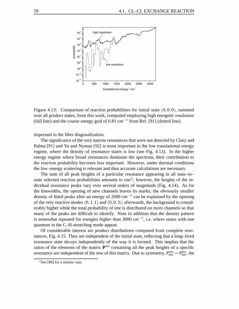
59 4.1. CL–CL EXCHANGE REACTION
Figure 4.13: Comparison of reaction probabilities for initial state (0,0,0), summedover all product states, from this work, computed employing high energetic resolution(full line) and the coarse energy grid of 0.81 cm−1 from Ref. [91] (dotted line).
important in the filter diagonalization.The significance of the very narrow resonances that were not detected by Clary and
Palma [91] and Yu and Nyman [92] is most important in the low translational energyregime, where the density of resonance states is low (see Fig. 4.13). In the higherenergy regime where broad resonances dominate the spectrum, their contribution tothe reaction probability becomes less important. However, under thermal conditionsthe low–energy scattering is relevant and thus accurate calculations are necessary.
The sum of all peak heights of a particular resonance appearing in all state–to–state selected reaction probabilities amounts to one2; however, the heights of the in-dividual resonance peaks vary over several orders of magnitude (Fig. 4.14). As forthe linewidths, the opening of new channels leaves its marks; the obviously smallerdensity of fitted peaks after an energy of 2000 cm−1 can be explained by the openingof the very reactive modes (0,1,1) and (0,0,3); afterwards, the background is consid-erably higher while the total probability of one is distributed on more channels so thatmany of the peaks are difficult to identify. Note in addition that the density patternis somewhat repeated for energies higher than 3000 cm−1, i.e. where states with onequantum in the C–H-stretching mode appear.
Of considerable interest are product distributions computed from complete reso-nances, Fig. 4.15. They are independent of the initial state, reflecting that a long–livedresonance state decays independently of the way it is formed. This implies that theratios of the elements of the matrix Pres containing all the peak heights of a specificresonance are independent of the row of this matrix. Due to symmetry, Pres
mn = Presnm , the
2See [88] for a similar case.
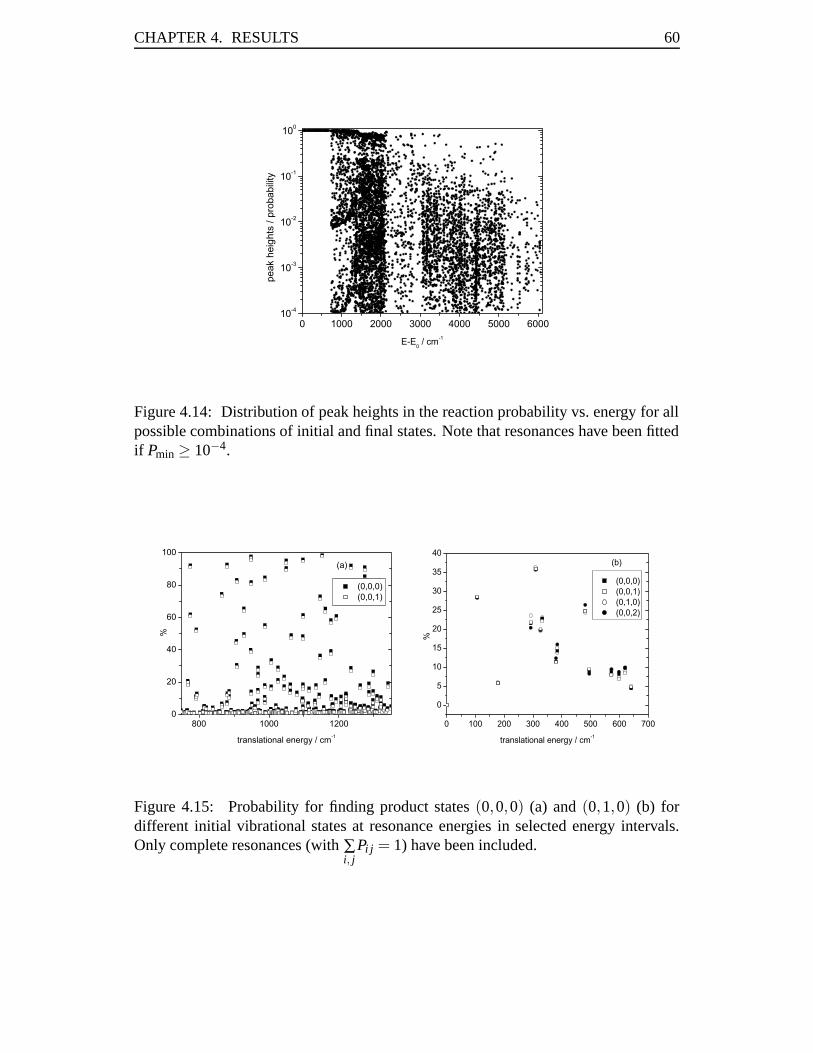
CHAPTER 4. RESULTS 60
Figure 4.14: Distribution of peak heights in the reaction probability vs. energy for allpossible combinations of initial and final states. Note that resonances have been fittedif Pmin ≥ 10−4.
Figure 4.15: Probability for finding product states (0,0,0) (a) and (0,1,0) (b) fordifferent initial vibrational states at resonance energies in selected energy intervals.Only complete resonances (with ∑
i, jPi j = 1) have been included.
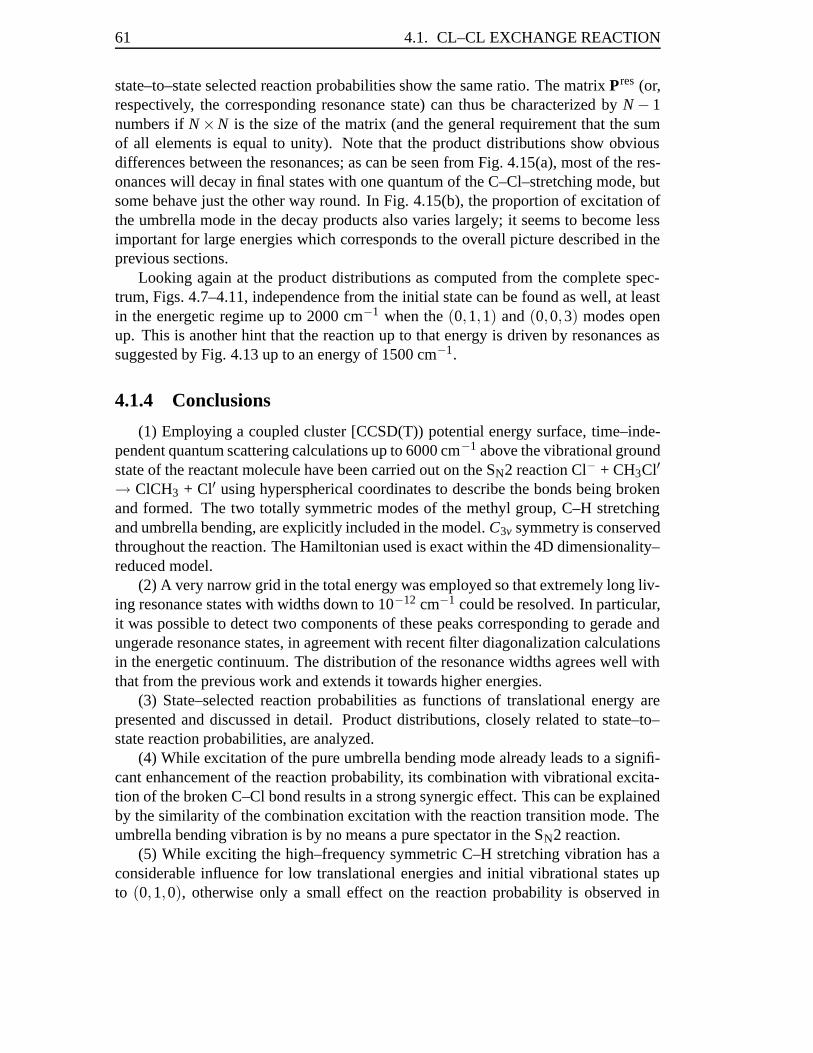
61 4.1. CL–CL EXCHANGE REACTION
state–to–state selected reaction probabilities show the same ratio. The matrix Pres (or,respectively, the corresponding resonance state) can thus be characterized by N − 1numbers if N ×N is the size of the matrix (and the general requirement that the sumof all elements is equal to unity). Note that the product distributions show obviousdifferences between the resonances; as can be seen from Fig. 4.15(a), most of the res-onances will decay in final states with one quantum of the C–Cl–stretching mode, butsome behave just the other way round. In Fig. 4.15(b), the proportion of excitation ofthe umbrella mode in the decay products also varies largely; it seems to become lessimportant for large energies which corresponds to the overall picture described in theprevious sections.
Looking again at the product distributions as computed from the complete spec-trum, Figs. 4.7–4.11, independence from the initial state can be found as well, at leastin the energetic regime up to 2000 cm−1 when the (0,1,1) and (0,0,3) modes openup. This is another hint that the reaction up to that energy is driven by resonances assuggested by Fig. 4.13 up to an energy of 1500 cm−1.
4.1.4 Conclusions
(1) Employing a coupled cluster [CCSD(T)) potential energy surface, time–inde-pendent quantum scattering calculations up to 6000 cm−1 above the vibrational groundstate of the reactant molecule have been carried out on the SN2 reaction Cl− + CH3Cl′→ ClCH3 + Cl′ using hyperspherical coordinates to describe the bonds being brokenand formed. The two totally symmetric modes of the methyl group, C–H stretchingand umbrella bending, are explicitly included in the model. C3v symmetry is conservedthroughout the reaction. The Hamiltonian used is exact within the 4D dimensionality–reduced model.
(2) A very narrow grid in the total energy was employed so that extremely long liv-ing resonance states with widths down to 10−12 cm−1 could be resolved. In particular,it was possible to detect two components of these peaks corresponding to gerade andungerade resonance states, in agreement with recent filter diagonalization calculationsin the energetic continuum. The distribution of the resonance widths agrees well withthat from the previous work and extends it towards higher energies.
(3) State–selected reaction probabilities as functions of translational energy arepresented and discussed in detail. Product distributions, closely related to state–to–state reaction probabilities, are analyzed.
(4) While excitation of the pure umbrella bending mode already leads to a signifi-cant enhancement of the reaction probability, its combination with vibrational excita-tion of the broken C–Cl bond results in a strong synergic effect. This can be explainedby the similarity of the combination excitation with the reaction transition mode. Theumbrella bending vibration is by no means a pure spectator in the SN2 reaction.
(5) While exciting the high–frequency symmetric C–H stretching vibration has aconsiderable influence for low translational energies and initial vibrational states upto (0,1,0), otherwise only a small effect on the reaction probability is observed in

CHAPTER 4. RESULTS 62
agreement with the spectator mode concept. However, this concept in questionable inso far as energy originally stored in the ν1 mode is released in the other modes of thereaction products. Thus, though quantitatively small, the role of the C–H mode in thereaction dynamics is not negligible.
(6) Product distributions of individual resonances can be calculated from their peakheights in different state–to–state reaction probabilities. It is found that the decay ofthe resonances is independent of the initial vibrational state of the reactant.
(7) The next step in studying the SN2 elementary reaction is to leave the collinearreaction pathway and to consider various directions of approximation of the nucle-ophile towards the methyl halide molecule. It is anticipated that the reaction proba-bility is strongly decreased. While the rotation of the methyl group around its axisof symmetry (A rotational constant) was already an object of investigation [89], therotation of the methyl halide molecule around an axis orthogonal to its axis of sym-metry, i.e. the motion connected with the B rotational constant, requires two differentcoordinate systems for reactants and products and the use of suitably adapted basissets.
4.2 Cl–Br Exchange Reaction
4.2.1 Abstract
The exothermic gas–phase SN2 reaction Cl− + CH3Br (v′1,v′2,v
′3) → ClCH3 (v1,v2,v3)
+ Br− and the corresponding endothermic reverse reaction have been studied by time–independent quantum scattering calculations in hyperspherical coordinates on a cou-pled cluster (CCSD(T)) potential energy surface. The dimensionality–reduced modeltakes four degrees of freedom into account (Cl–C and C–Br stretching modes (quantumnumbers v′3 and v3); totally symmetric modes of the methyl group, i.e. C–H stretch-ing (v′1 and v1) and umbrella bending vibrations (v′2 and v2)). Diagonalization of theHamiltonian was performed using the Lanczos algorithm with a variation of partial re-orthogonalization. A narrow grid in the total energy was employed so that long–livingresonance states could be resolved and extracted. While excitation of the reactant um-brella bending mode already leads to a considerable enhancement of the reaction prob-ability, its combination with vibrational excitation of the broken C–Br bond, (0,1,1),results in a strong synergic effect that can be rationalized by the similarity with the clas-sical transitional normal mode. Exciting the C–H stretch has a non–negligible effecton the reaction probability, while for larger translational energies this mode followsthe expected spectator–like behavior. Combination of C–Br stretch and symmetricC–H stretch, (1,0,1), does not show a cooperative effect. Contrary to the spectatormode concept, energy originally stored in the C–H stretching mode is by no meansconserved, but released in other modes of the reaction products. Products are mostlikely formed in states with a high degree of excitation in the new C–Cl bond, whilethe internal modes of the methyl group are less important. Reactants with combined

63 4.2. CL–BR EXCHANGE REACTION
umbrella/C–Br stretch excitation, (0,1,1), may yield products with two quanta in theumbrella mode.
4.2.2 Introduction
In this section, we present a four–dimensional (4D) study of the exothermic reaction
Cl− +CH3Br → ClCH3 +Br− (4.4)
and the corresponding endothermic reverse reaction. The first quantum mechanicalstudy on a gas–phase SN2 reaction was performed by Wang, Goldfield and Hase [100]who studied the time–dependent dynamics of a two–dimensional (2D) wave packetin a model with the minimum number of degrees of freedom (carbon–halogen bondsbeing formed and broken). Clary [13] could obtain the thermal rate constant from adimensionality–reduced three–dimensional (3D) quantum model with an approximateHamiltonian for the umbrella bending coordinate and found good agreement with ex-periment. Reaction cross sections in a 2D model were calculated and analyzed bySchmatz and Clary [31]. A 2D investigation of resonance lifetimes for the complexesCl− · · ·CH3Br (entrance channel) and ClCH3 · · ·Br− (exit channel), obtained directlyas the imaginary parts of the complex eigenvalues, E = Eres − i
2Γ, of a complex–symmetric Hamiltonian matrix was reported by Schmatz et al. [32] who employeda coupled–cluster (CCSD(T)) potential energy surface in conjunction with the filterdiagonalization method. The five stationary points (reactants, products, saddle pointand the two intermediate complexes) on this surface had already been reported inRef. [101]. In a recent paper, Schmatz [102] reported the linewidths for the samesystem in a four–mode model on an extended PES. The four–dimensional model alsoincludes the two totally symmetric vibrations of the methyl group (C–H stretch andumbrella bend). The vast majority of bound states and many resonance states up to thefirst overtone of the symmetric stretching vibration in the exit channel complex havebeen calculated, analyzed and assigned four quantum numbers. The resonances wereclassified into entrance channel, exit channel and delocalized states. It could be shownthat the widths of the resonances within a small energy window cover more than sixorders of magnitude. In addition to a majority of Feshbach–type resonances, exceed-ingly long-lived shape resonances were found which are associated with the entrancechannel and can only decay by tunneling. The state–selective decay of the resonanceswas studied in detail. The linewidths of the resonances and thus the coupling to theenergetic continuum increase with excitation in any mode. Due to the strong mixingof the many progressions in the intermolecular stretching modes of the intermediatecomplexes, this increase as a function of the corresponding quantum numbers is notmonotonic, but exhibits pronounced fluctuations.
In the present work, we use the same dimensionality–reduced Hamiltonian as em-ployed in Ref. [102]. A rigorous quantum mechanical treatment appears to be im-possible at present because for an exact description of the Cl− + CH3Br SN2 system,
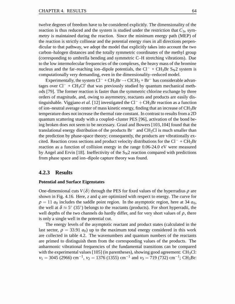
CHAPTER 4. RESULTS 64
twelve degrees of freedom have to be considered explicitly. The dimensionality of thereaction is thus reduced and the system is studied under the restriction that C3v sym-metry is maintained during the reaction. Since the minimum energy path (MEP) ofthe reaction is strictly collinear and the potential energy rises in all directions perpen-dicular to that pathway, we adopt the model that explicitly takes into account the twocarbon–halogen distances and the totally symmetric coordinates of the methyl group(corresponding to umbrella bending and symmetric C–H stretching vibrations). Dueto the low intermolecular frequencies of the complexes, the heavy mass of the brominenucleus and the far–reaching ion–dipole potentials, the Cl− + CH3Br SN2 system iscomputationally very demanding, even in the dimensionality–reduced model.
Experimentally, the system Cl− + CH3Br → ClCH3 + Br− has considerable advan-tages over Cl− + CH3Cl′ that was previously studied by quantum mechanical meth-ods [79]. The former reaction is faster than the symmetric chlorine exchange by threeorders of magnitude, and, owing to asymmetry, reactants and products are easily dis-tinguishable. Viggiano et al. [12] investigated the Cl− +CH3Br reaction as a functionof ion–neutral average center of mass kinetic energy, finding that an increase of CH3Brtemperature does not increase the thermal rate constant. In contrast to results from a 2Dquantum scattering study with a coupled–cluster PES [96], activation of the bond be-ing broken does not seem to be necessary. Graul and Bowers [103,104] found that thetranslational energy distribution of the products Br− and CH3Cl is much smaller thanthe prediction by phase-space theory; consequently, the products are vibrationally ex-cited. Reaction cross sections and product velocity distributions for the Cl− + CH3Brreaction as a function of collision energy in the range 0.06-24.0 eV were measuredby Angel and Ervin [18]. Ineffectivity of the SN2 reaction compared with predictionsfrom phase space and ion–dipole capture theory was found.
4.2.3 Results
Potential and Surface Eigenstates
One-dimensional cuts V (δ ) through the PES for fixed values of the hyperradius ρ areshown in Fig. 4.16. Here, z and q are optimized with respect to energy. The curve forρ = 11 a0 includes the saddle point region. In the asymptotic region, here at 34 a0,the well at δ ≈ 5◦ (35◦) belongs to the reactants (products). For short hyperradii, thewell depths of the two channels do hardly differ, and for very short values of ρ , thereis only a single well in the potential cut.
The energy levels of the asymptotic reactant and product states (calculated in thelast sector, ρ = 33.91 a0) up to the maximum total energy considered in this workare collected in table 4.2. The wavenumbers and quantum numbers of the reactantsare primed to distinguish them from the corresponding values of the products. Theanharmonic vibrational frequencies of the fundamental transitions can be comparedwith the experimental values [105] (in parentheses), showing good agreement: CH3Cl:ν1 = 3045 (2966) cm−1, ν2 = 1376 (1355) cm−1 and ν3 = 719 (732) cm−1; CH3Br:
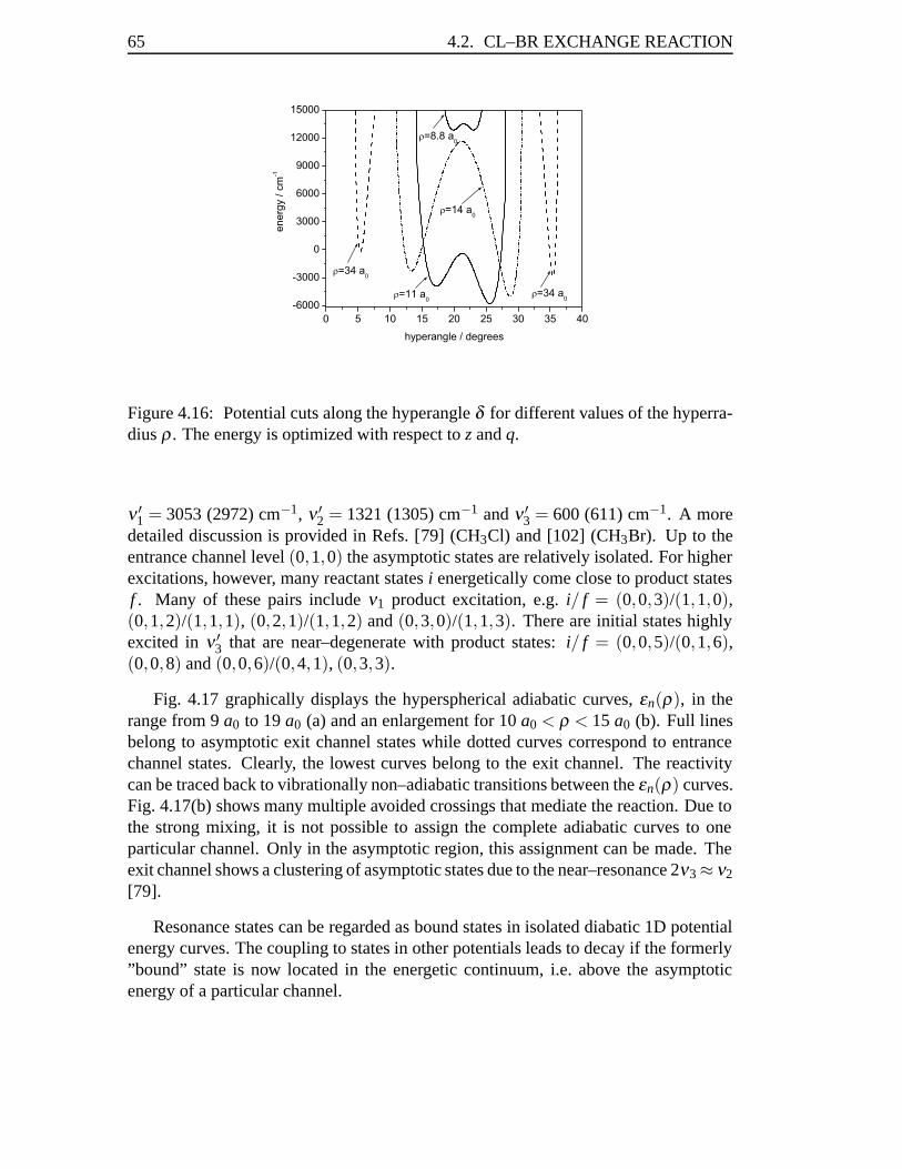
65 4.2. CL–BR EXCHANGE REACTION
Figure 4.16: Potential cuts along the hyperangle δ for different values of the hyperra-dius ρ . The energy is optimized with respect to z and q.
ν ′1 = 3053 (2972) cm−1, ν ′
2 = 1321 (1305) cm−1 and ν ′3 = 600 (611) cm−1. A more
detailed discussion is provided in Refs. [79] (CH3Cl) and [102] (CH3Br). Up to theentrance channel level (0,1,0) the asymptotic states are relatively isolated. For higherexcitations, however, many reactant states i energetically come close to product statesf . Many of these pairs include ν1 product excitation, e.g. i/ f = (0,0,3)/(1,1,0),(0,1,2)/(1,1,1), (0,2,1)/(1,1,2) and (0,3,0)/(1,1,3). There are initial states highlyexcited in ν ′
3 that are near–degenerate with product states: i/ f = (0,0,5)/(0,1,6),(0,0,8) and (0,0,6)/(0,4,1), (0,3,3).
Fig. 4.17 graphically displays the hyperspherical adiabatic curves, εn(ρ), in therange from 9 a0 to 19 a0 (a) and an enlargement for 10 a0 < ρ < 15 a0 (b). Full linesbelong to asymptotic exit channel states while dotted curves correspond to entrancechannel states. Clearly, the lowest curves belong to the exit channel. The reactivitycan be traced back to vibrationally non–adiabatic transitions between the εn(ρ) curves.Fig. 4.17(b) shows many multiple avoided crossings that mediate the reaction. Due tothe strong mixing, it is not possible to assign the complete adiabatic curves to oneparticular channel. Only in the asymptotic region, this assignment can be made. Theexit channel shows a clustering of asymptotic states due to the near–resonance 2ν3 ≈ ν2
[79].
Resonance states can be regarded as bound states in isolated diabatic 1D potentialenergy curves. The coupling to states in other potentials leads to decay if the formerly”bound” state is now located in the energetic continuum, i.e. above the asymptoticenergy of a particular channel.
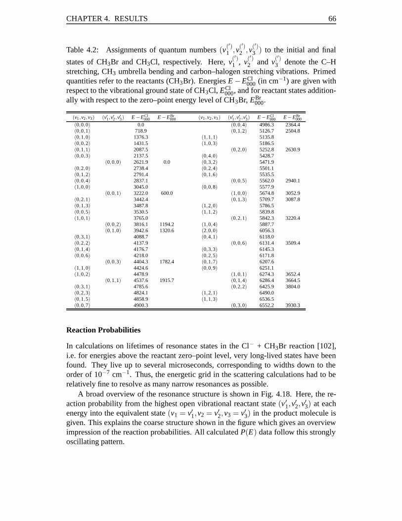
CHAPTER 4. RESULTS 66
Table 4.2: Assignments of quantum numbers (v(′)1 ,v(′)
2 ,v(′)3 ) to the initial and final
states of CH3Br and CH3Cl, respectively. Here, v(′)1 , v(′)
2 and v(′)3 denote the C–H
stretching, CH3 umbrella bending and carbon–halogen stretching vibrations. Primedquantities refer to the reactants (CH3Br). Energies E −ECl
000 (in cm−1) are given withrespect to the vibrational ground state of CH3Cl, ECl
000, and for reactant states addition-ally with respect to the zero–point energy level of CH3Br, EBr
000.
(v1,v2,v3) (v′1,v′2,v′3) E −ECl000 E −EBr
000 (v1,v2,v3) (v′1,v′2 ,v′3) E −ECl000 E −EBr
000
(0,0,0) 0.0 (0,0,4) 4986.3 2364.4(0,0,1) 718.9 (0,1,2) 5126.7 2504.8(0,1,0) 1376.3 (1,1,1) 5135.8(0,0,2) 1431.5 (1,0,3) 5186.5(0,1,1) 2087.5 (0,2,0) 5252.8 2630.9(0,0,3) 2137.5 (0,4,0) 5428.7
(0,0,0) 2621.9 0.0 (0,3,2) 5471.9(0,2,0) 2738.4 (0,2,4) 5501.1(0,1,2) 2791.4 (0,1,6) 5535.5(0,0,4) 2837.1 (0,0,5) 5562.0 2940.1(1,0,0) 3045.0 (0,0,8) 5577.9
(0,0,1) 3222.0 600.0 (1,0,0) 5674.8 3052.9(0,2,1) 3442.4 (0,1,3) 5709.7 3087.8(0,1,3) 3487.8 (1,2,0) 5786.5(0,0,5) 3530.5 (1,1,2) 5839.8(1,0,1) 3765.0 (0,2,1) 5842.3 3220.4
(0,0,2) 3816.1 1194.2 (1,0,4) 5887.7(0,1,0) 3942.6 1320.6 (2,0,0) 6056.3
(0,3,1) 4088.7 (0,4,1) 6118.0(0,2,2) 4137.9 (0,0,6) 6131.4 3509.4(0,1,4) 4176.7 (0,3,3) 6145.3(0,0,6) 4218.0 (0,2,5) 6171.8
(0,0,3) 4404.3 1782.4 (0,1,7) 6207.6(1,1,0) 4424.6 (0,0,9) 6251.1(1,0,2) 4478.9 (1,0,1) 6274.3 3652.4
(0,1,1) 4537.6 1915.7 (0,1,4) 6286.4 3664.5(0,3,1) 4785.6 (0,2,2) 6425.9 3804.0(0,2,3) 4824.1 (1,2,1) 6490.0(0,1,5) 4858.9 (1,1,3) 6536.5(0,0,7) 4900.3 (0,3,0) 6552.2 3930.3
Reaction Probabilities
In calculations on lifetimes of resonance states in the Cl− + CH3Br reaction [102],i.e. for energies above the reactant zero–point level, very long-lived states have beenfound. They live up to several microseconds, corresponding to widths down to theorder of 10−7 cm−1. Thus, the energetic grid in the scattering calculations had to berelatively fine to resolve as many narrow resonances as possible.
A broad overview of the resonance structure is shown in Fig. 4.18. Here, the re-action probability from the highest open vibrational reactant state (v′1,v
′2,v
′3) at each
energy into the equivalent state (v1 = v′1,v2 = v′2,v3 = v′3) in the product molecule isgiven. This explains the coarse structure shown in the figure which gives an overviewimpression of the reaction probabilities. All calculated P(E) data follow this stronglyoscillating pattern.

67 4.2. CL–BR EXCHANGE REACTION
Figure 4.17: Hyperspherical adiabatic curves. Shown are all Nch = 150 curves whereof96 belong to asymptotic exit channel states while 54 are pertinent to entrance channelstates. The classical asymptotic limit of the PES is set to zero. While Fig. 3(a) givesthe full energy range covered by our calculations, Fig. 3(b) displays only a small partincluding numerous avoided crossings between the hyperspherical adiabatic curvesthat mediate the non–adiabatic transitions between the different vibrational states.
Figure 4.18: The reaction probability P(E) as a function of energy E is stronglydominated by scattering resonances. Shown are the diagonal state–to–state reactionprobabilities Pi, f (E), i.e. v′i = vi, i = 1,2,3 for the highest reactant channel (v′1,v
′2,v
′3)
at energy E.

CHAPTER 4. RESULTS 68
To facilitate the comparison between different initial vibrational states, the P(E)curves are averaged over 80 cm−1 so that each point is the arithmetic mean of allprobabilities in the interval [E−Δ,E +Δ] with Δ = 40 cm−1. All initial–state selectedP(E) curves shown in the following and all product distributions (which are related tostate–to–state reaction probabilities Pi, f (E)) are averaged according to this procedure.
• The exothermic reaction Cl− + CH3Br
Fig. 4.19(a) shows the initial–state selected reaction probabilities summed over allproduct states as a function of initial translational energy,
Pi(E) = ∑f
Pi, f (E) = ∑f
|Si, f |2. (4.5)
The energetic ranges of the curves are different because the data are not shown asfunctions of total energy; to recover the probabilities as functions of total energy, theindividual curves must be shifted by the corresponding energy levels quoted in ta-ble 4.2. There is a clear distinction between three groups of curves. The first groupcontains initial vibrational states without excitation in the C–Br bond. Here, P(E) isfar below 0.1. The second group contains those initial states with one quantum ofinternal energy in the C–Br stretching mode ν ′
3; here, the reaction probabilities areconsiderably increased. Finally, after a clear gap, the third group contains P(E) curvescorresponding to initial vibrational states with v′3 ≥ 2. These curves are found in theprobability interval from 0.5 to 0.8 with a tendency to saturation at the latter valuewhich is still below the maximum value of 1.0 that should be reached for a classicalbarrierless reaction.
Fig. 4.19(b) displays the probability for reaction out of the vibrational ground statewhich rises exponentially with a pronounced coarse structure. Exciting the umbrellabending mode ν ′
2 in the reactant CH3Br yields a significant increase of P(E). Interest-ingly, excitation of the high–frequency C–H stretching mode ν ′
1 shows quantitativelya very similar effect. This observation leads to the conclusion that both totally sym-metric modes of the methyl group have a comparable influence on the reactivity in theCl− + CH3Br reaction. Putting two quanta in the umbrella bending mode results in analmost linear increase of P(E) compared to excitation v′2 = 1. It should be pointed outthat the coarse shape of all curves displayed in Fig. 4.19(b) is quite similar exhibitinga dip at about 750 cm−1 of translational energy.
The well–known ’spectator’ mode concept states that a bond which is not directlyinvolved in the reaction can be treated adiabatically and does not show a significantinfluence on the reactivity. The high–frequency C–H stretch is often regarded as a pro-totypical example of a spectator mode. The mode is present both in reactants and inproducts and, owing to its large frequency, the coupling to the other modes is expectedto be weak. Surprisingly, despite the fairly small influence of these ’spectator’ modeson thermal reactions (due to their low population), they should be included if one aimsat a detailed understanding of the underlying dynamics: From the present calculations,

69 4.2. CL–BR EXCHANGE REACTION
Figure 4.19: Initial state–selected probabilities Pi(E) for the exothermic reaction Cl−+ CH3Br (v′1,v
′2,v
′3)→ ClCH3 + Br− as functions of translational energy Etrans. The
data is smoothed over intervals of 80 cm−1. Pi, f (E) is summed over all accessibleproduct channels f . (a) Overview, (b) without excitation in ν ′
3, (c) one quantum in ν ′3,
(d) two or more quanta in ν ′3.
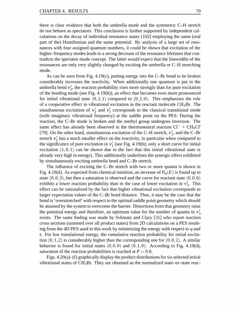
CHAPTER 4. RESULTS 70
there is clear evidence that both the umbrella mode and the symmetric C–H stretchdo not behave as spectators. This conclusion is further supported by independent cal-culations on the decay of individual resonance states [102] employing the same (realpart of the) Hamiltonian and the same potential. By analysis of a large set of reso-nances with four assigned quantum numbers, it could be shown that excitation of thehigher–frequency modes leads to a strong decrease of the resonance lifetimes that con-tradicts the spectator mode concept. The latter would expect that the linewidths of theresonances are only very slightly changed by exciting the umbrella or C–H stretchingmode.
As can be seen from Fig. 4.19(c), putting energy into the C–Br bond to be brokenconsiderably increases the reactivity. When additionally one quantum is put in theumbrella bend ν ′
2, the reaction probability rises more strongly than for pure excitationof the bending mode (see Fig. 4.19(b)), an effect that becomes even more pronouncedfor initial vibrational state (0,2,1) compared to (0,2,0). This emphasizes the roleof a cooperative effect in vibrational excitation in the reactant molecule CH3Br. Thesimultaneous excitation of ν ′
2 and ν ′3 corresponds to the classical transitional mode
(with imaginary vibrational frequency) at the saddle point on the PES: During thereaction, the C–Br mode is broken and the methyl group undergoes inversion. Thesame effect has already been observed in the thermoneutral reaction Cl− + CH3Cl′[79]. On the other hand, simultaneous excitation of the C–H stretch, ν ′
1, and the C–Brstretch ν ′
3 has a much smaller effect on the reactivity, in particular when compared tothe significance of pure excitation in ν ′
1 (see Fig. 4.19(b); only a short curve for initialexcitation (1,0,1) can be shown due to the fact that this initial vibrational state isalready very high in energy). This additionally underlines the synergic effect exhibitedby simultaneously exciting umbrella bend and C–Br stretch.
The influence of exciting the C–Br stretch with two or more quanta is shown inFig. 4.19(d). As expected from chemical intuition, an increase of Pm(E) is found up tostate (0,0,3), but then a saturation is observed and the curve for reactant state (0,0,6)exhibits a lower reaction probability than in the case of lower excitation in ν ′
3. Thiseffect can be rationalized by the fact that higher vibrational excitation corresponds tolarger expectation values of the C–Br bond distance. Thus, it may be the case that thebond is ’overstretched’ with respect to the optimal saddle point geometry which shouldbe attained by the system to overcome the barrier. Distortions from that geometry raisethe potential energy and therefore, an optimum value for the number of quanta in ν ′
3exists. The same finding was made by Schmatz and Clary [31] who report reactioncross sections (summed over all product states) from 2D calculations on a PES result-ing from the 4D PES used in this work by minimizing the energy with respect to q andz. For low translational energy, the cumulative reaction probability for initial excita-tion (0,1,2) is considerably higher than the corresponding one for (0,0,2). A similarbehavior is found for initial states (0,0,0) and (0,1,0). According to Fig. 4.19(d),saturation of the reaction probabilities is reached at P = 0.8.
Figs. 4.20(a)–(f) graphically display the product distributions for six selected initialvibrational states of CH3Br. They are obtained as the normalized state–to–state reac-

71 4.2. CL–BR EXCHANGE REACTION
tion probabilities, Pi, f (E)/Pi(E). Absolute state–to–state reaction probabilities canbe obtained by multiplying the data from Figs. 4.19 with the percentage amounts ofFigs. 4.20. Note that all product states with a negligible population are not shown inthe figures.
At very low translational energies, reaction out of the CH3Br ground state (seeFig. 4.20(a)) is most likely to end in product state (0,0,3) whose contribution decreasesto ca. 20 % and then on average remains constant. When the (0,1,2) product channelopens, it becomes dominant, but for higher translational energies decreases to smallervalues. The (0,0,2) CH3Cl state is populated fairly low at small Etrans but for highercollision energies the percentage amount of this product channel increases to morethan 30 %. After opening of the (0,0,4) product channel, its population rises to morethan 25 %, but decreases for higher energies. In summary, for reaction out of CH3Brin its vibrational ground state, products with the C–Cl stretch excited by 2–4 quantaare formed. In agreement with the observation by Graul and Bowers [103, 104], theproducts are vibrationally hot.
Putting one quantum of energy in the bond being broken, i.e. the C–Br stretchingmode (Fig. 4.20(b)), results in a very similar picture. The (0,0,3) product curve startsat ca. 20 % and slightly rises for larger Etrans. The (0,0,2) channel starts at ca. 5 %and strongly increases, with pronounced oscillations, up to 40 % in the energy regimeconsidered. The (0,0,4) state is initially relative important, while it becomes less pop-ulated at higher energies. The combination level (0,1,1) exhibits a contribution ofalmost constantly more than 10 %. As for reactant state (0,0,0), the product channel(0,1,2) is initially most important, but becomes much less significant at larger trans-lational energies. Note that all product levels shown in Fig. 4.20(b) are energeticallylocated below the reactant state. The product channel (0,0,5) is insignificant.
For initially one quantum in the umbrella bending vibration ν ′2, (Fig. 4.20(c)), prod-
uct channels with pure ν ′2 excitation are most likely formed only at lower translational
energies. Product states (0,0,3) and (0,0,4) are on average almost equally probablewhile showing stronger oscillations. The same observation is made for the (0,0,5)state whose average contribution is considerably higher, however. The CH3Cl com-bination modes (0,1,2), (0,1,3) and (0,1,4) show large contributions at small E trans,but then decay fast to values below 5 %. In summary, C–Cl stretching excitation inthe products is strongly favored. For small translational energies, the umbrella modebehaves adiabatically, i.e. the energy in this mode is conserved and a considerable partof the collision energy is transformed into vibrational energy (T → V process). Forlarge translational energies, the energy originally stored in ν ′
2 is almost completelyredistributed.
For reactants in state (0,1,1) (Fig. 4.20(d)), overall a similar behavior is observed.Product C–Cl stretching states are strongly populated, in particular state (0,0,5) withalmost up to 30 %, but also state (0,0,4) and to much less extend (0,0,3). Prod-uct combination levels with v2 = 1 are initially quite significant ((0,1,3), (0,1,4) and(0,1,5) start at about 10, 15 and 8 %, respectively), but then show a decreasing ten-dency. Surprisingly, product channel (0,2,1) starts at more than 10 % and then further
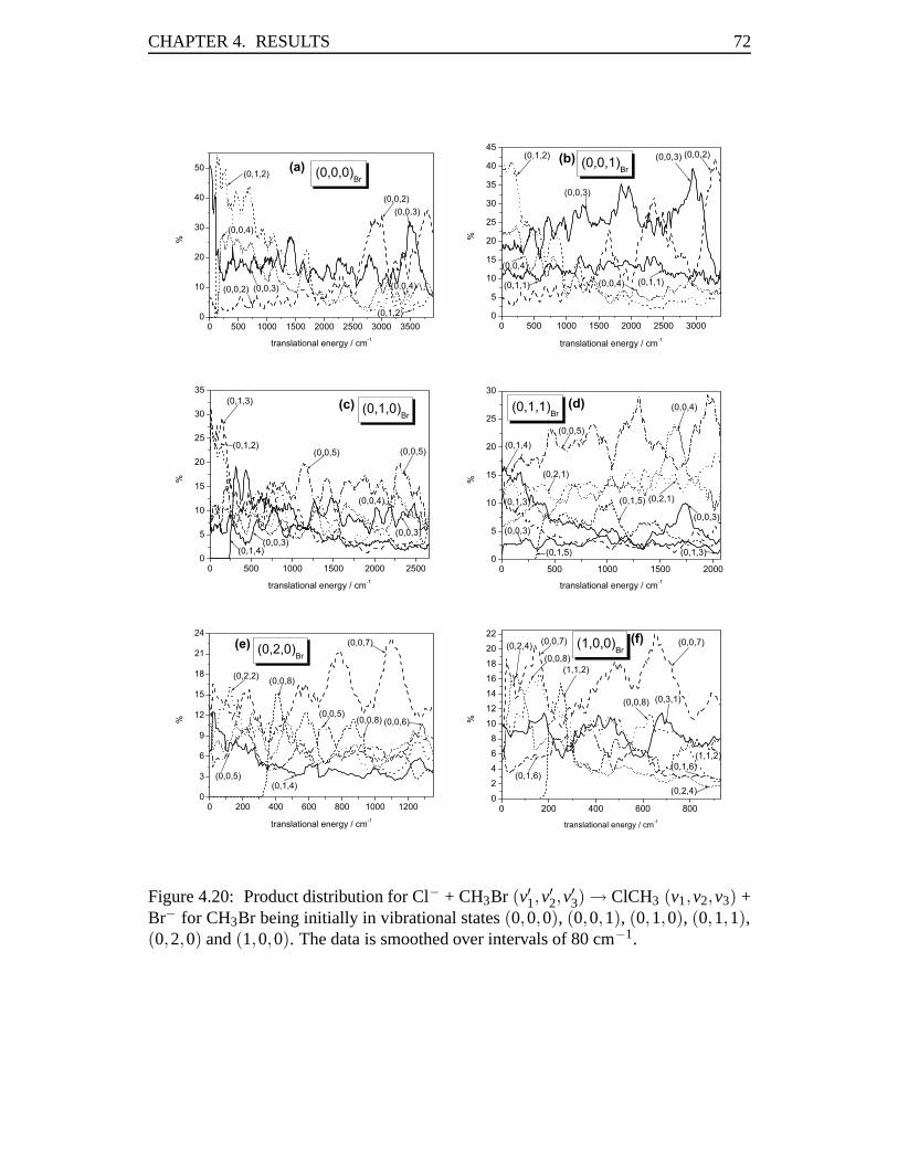
CHAPTER 4. RESULTS 72
Figure 4.20: Product distribution for Cl− + CH3Br (v′1,v′2,v
′3) → ClCH3 (v1,v2,v3) +
Br− for CH3Br being initially in vibrational states (0,0,0), (0,0,1), (0,1,0), (0,1,1),(0,2,0) and (1,0,0). The data is smoothed over intervals of 80 cm−1.

73 4.2. CL–BR EXCHANGE REACTION
increases. With Δv2 = +1 this is a T → V process. This points out that the umbrellamode clearly is not a spectator mode and that the combination mode exhibits a partic-ularly high reactivity. The Δv2 = +1 transition is possible only when additionally theC–Br mode is excited.
Initially two quanta in the umbrella mode, (0,2,0) (Fig. 4.20(e)), again favor theproduct channels (0,0,n) close in energy. Most significant is state (0,0,7) startingat ca. 15 % and then increasing with strong oscillations. The contribution of chan-nel (0,0,8) rises – after its opening – to almost 15 %, but decreases for higher Etrans.Product channels (0,0,5) and (0,0,6) show a relative similar behavior, but are lessimportant compared to state (0,0,7). The isoenergetic product channels (0,1,4) and(0,2,2) initially show significant contributions which for higher energies become lessimportant, in agreement with initial excitation (0,1,0). Overall, the product distribu-tion for (0,2,0) is shifted by two quanta in ν3 compared to initial state (0,1,0). Thisis not surprising because for CH3Cl we have ν2 ≈ 2ν3. Thus, the translational energydistribution is not changed.
CH3Br initially excited with one quantum in the symmetric C–H stretching modeν ′
1 (Fig. 4.20(f)) results in the dominant product channel (0,0,7) and a significantcontribution of state (0,0,8). The isoenergetic channels (0,1,6), (0,2,4) and (0,3,1)are also important. The only product state with energy stored in ν1 is (1,1,2) that afterits opening rises to 15 % and then decreases to on average about 6 %. As can be seenfrom Fig. 4.20(f), the probability to find products with the umbrella mode excited, inparticular in combination with the C–Cl stretch, is high. This underlines the active roleof this mode in the reaction.
• The endothermic reaction Br− + CH3Cl
Fig. 4.21 graphically displays the initial state–selected reaction probabilities forthe reverse, endothermic reaction Br− + CH3Cl (v1,v2,v3) → BrCH3 (v′1,v
′2,v
′3) +
Cl−. Here, P(E) is much smaller, and Fig. 4.21(a) is given with a logarithmic scale. Itis relatively difficult to divide the curves into groups.
Fig. 4.21(b) contains the isolated P(E) curve for reaction out of the vibrationalground state of CH3Cl. Clearly, it is non–zero only when the total energy is largerthan that of the first state at the product side. The reaction probability rises less thanexponentially. Fig. 4.21(a) contains four other relatively low probability curves thatall belong to initial vibrational states with v1 = 1. Owing to the high frequency ofthis mode, the curves start at Etrans = 0. Excitation of ν1 increases the reactivity. Thiseffect is enhanced by simultaneous excitation of the C–Cl stretch, ν3, and the umbrellabend, ν2. Note that putting one quantum of energy in the umbrella bending moderesults in a similar but slightly larger reaction probability than one quantum in themode corresponding to the bond that is broken. The C–H stretch cannot be consideredas a spectator because the energy originally stored in this mode is used to overcomethe large reaction barrier.
Fig. 4.21(c) gives the reaction probabilities for pure initial bending states (0,v2,0)with v2 = 1,2,3 and for the combined excitation of ν2 and ν3, (0,1,1). Also shown is

CHAPTER 4. RESULTS 74
Figure 4.21: Initial state–selected probabilities Pi(E) for the endothermic reactionBr− + CH3Cl (v1,v2,v3) → BrCH3 + Cl− as functions of translational energy Etrans.The data is smoothed over intervals of 80 cm−1. Pi, f (E) is summed over all acces-sible product channels f . (a) Overview, (b) reaction out of the vibrational groundstate and states with excitation v′1 = 1, (c) reaction out of states (0,0,1), (0,1,1) and(0,v2,0), v2 = 1,2,3, (d) higher excitation in ν3 and combination modes (0,v2,v3);curves (0,1,1) and (0,3,0) are also shown for comparison.
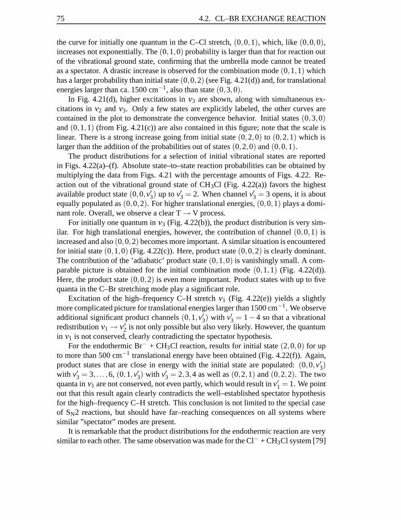
75 4.2. CL–BR EXCHANGE REACTION
the curve for initially one quantum in the C–Cl stretch, (0,0,1), which, like (0,0,0),increases not exponentially. The (0,1,0) probability is larger than that for reaction outof the vibrational ground state, confirming that the umbrella mode cannot be treatedas a spectator. A drastic increase is observed for the combination mode (0,1,1) whichhas a larger probability than initial state (0,0,2) (see Fig. 4.21(d)) and, for translationalenergies larger than ca. 1500 cm−1, also than state (0,3,0).
In Fig. 4.21(d), higher excitations in ν3 are shown, along with simultaneous ex-citations in ν2 and ν3. Only a few states are explicitly labeled, the other curves arecontained in the plot to demonstrate the convergence behavior. Initial states (0,3,0)and (0,1,1) (from Fig. 4.21(c)) are also contained in this figure; note that the scale islinear. There is a strong increase going from initial state (0,2,0) to (0,2,1) which islarger than the addition of the probabilities out of states (0,2,0) and (0,0,1).
The product distributions for a selection of initial vibrational states are reportedin Figs. 4.22(a)–(f). Absolute state–to–state reaction probabilities can be obtained bymultiplying the data from Figs. 4.21 with the percentage amounts of Figs. 4.22. Re-action out of the vibrational ground state of CH3Cl (Fig. 4.22(a)) favors the highestavailable product state (0,0,v′3) up to v′3 = 2. When channel v′3 = 3 opens, it is aboutequally populated as (0,0,2). For higher translational energies, (0,0,1) plays a domi-nant role. Overall, we observe a clear T → V process.
For initially one quantum in ν3 (Fig. 4.22(b)), the product distribution is very sim-ilar. For high translational energies, however, the contribution of channel (0,0,1) isincreased and also (0,0,2) becomes more important. A similar situation is encounteredfor initial state (0,1,0) (Fig. 4.22(c)). Here, product state (0,0,2) is clearly dominant.The contribution of the ’adiabatic’ product state (0,1,0) is vanishingly small. A com-parable picture is obtained for the initial combination mode (0,1,1) (Fig. 4.22(d)).Here, the product state (0,0,2) is even more important. Product states with up to fivequanta in the C–Br stretching mode play a significant role.
Excitation of the high–frequency C–H stretch ν1 (Fig. 4.22(e)) yields a slightlymore complicated picture for translational energies larger than 1500 cm−1. We observeadditional significant product channels (0,1,v′3) with v′3 = 1− 4 so that a vibrationalredistribution ν1 → ν ′
2 is not only possible but also very likely. However, the quantumin ν1 is not conserved, clearly contradicting the spectator hypothesis.
For the endothermic Br− + CH3Cl reaction, results for initial state (2,0,0) for upto more than 500 cm−1 translational energy have been obtained (Fig. 4.22(f)). Again,product states that are close in energy with the initial state are populated: (0,0,v′3)with v′3 = 3, . . . ,6, (0,1,v′3) with v′3 = 2,3,4 as well as (0,2,1) and (0,2,2). The twoquanta in ν1 are not conserved, not even partly, which would result in v′1 = 1. We pointout that this result again clearly contradicts the well–established spectator hypothesisfor the high–frequency C–H stretch. This conclusion is not limited to the special caseof SN2 reactions, but should have far–reaching consequences on all systems wheresimilar ”spectator” modes are present.
It is remarkable that the product distributions for the endothermic reaction are verysimilar to each other. The same observation was made for the Cl− + CH3Cl system [79]
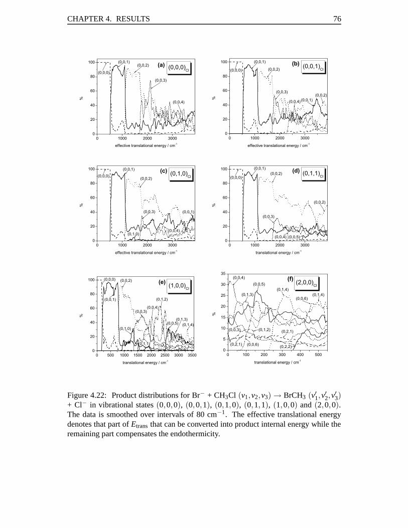
CHAPTER 4. RESULTS 76
Figure 4.22: Product distributions for Br− + CH3Cl (v1,v2,v3) → BrCH3 (v′1,v′2,v
′3)
+ Cl− in vibrational states (0,0,0), (0,0,1), (0,1,0), (0,1,1), (1,0,0) and (2,0,0).The data is smoothed over intervals of 80 cm−1. The effective translational energydenotes that part of Etrans that can be converted into product internal energy while theremaining part compensates the endothermicity.
77 4.2. CL–BR EXCHANGE REACTION
Figure 4.23: Comparison between reactions Cl− + CH3Y (v1,v2,v3) → ClCH3 + Y−with Y = Cl and Br. The initial quantum states of the methyl halide molecule are(0,0,0) and (1,0,0).
and can be rationalized by the long lifetimes of the resonance states. Once formed, thestate ”looses its memory” and decays independently of its origin. For higher–lyingresonance levels, in the region of increasing densities of states, the product distribu-tions are more complicated. This statement is obviously also valid for the exothermicreaction Cl− + CH3Br with the high–lying product states.
Comparison with the Thermoneutral Reaction Cl− + CH3Cl′
In Fig. 4.23, reactions of a chloride anion with either CH3Cl and CH3Br, both in theirvibrational ground state, are compared. Also shown in this figure are the reactionprobabilities for initial excitation of the symmetric C–H stretching modes in CH3Cland CH3Br, respectively. For CH3Br, the reaction probability out of the vibrationalground state is two orders of magnitude larger for small translational energies and oneorder of magnitude at Etrans = 3500 cm−1. Both P(E) curves for the vibrational groundstate on average follow exponential laws, P(Etrans) = AeαEtrans with ACH3Cl = 1.3 ·10−5,ACH3Br = 2.3 ·10−3, αCH3Cl = 1.55 ·10−3 1/cm−1 and αCH3Br = 0.82 ·10−3 1/cm−1.
Putting one quantum in the symmetric C–H stretching mode increases P(E) forCH3Cl at low Etrans by about two orders of magnitude, while this mode becomes aspectator for energies higher than ca. 1700 cm−1. For CH3Br, the corresponding in-crease for small Etrans is only one order of magnitude and the spectator mode behaviorsets in already at ca. 900 cm−1. Obviously, the missing net barrier in the Cl− + CH3Brpotential is the reason for the different behavior. The barrier in the Cl− + CH3Cl po-tential renders the C–H mode more important as an energy reservoir for surmountingthe barrier. The difference between the Etrans values where the spectator–like behavior
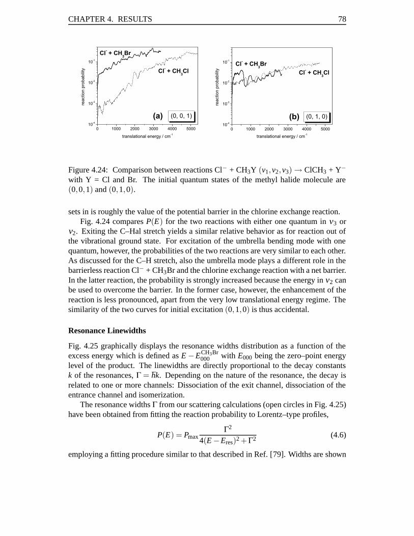
CHAPTER 4. RESULTS 78
Figure 4.24: Comparison between reactions Cl− + CH3Y (v1,v2,v3) → ClCH3 + Y−with Y = Cl and Br. The initial quantum states of the methyl halide molecule are(0,0,1) and (0,1,0).
sets in is roughly the value of the potential barrier in the chlorine exchange reaction.Fig. 4.24 compares P(E) for the two reactions with either one quantum in ν3 or
ν2. Exiting the C–Hal stretch yields a similar relative behavior as for reaction out ofthe vibrational ground state. For excitation of the umbrella bending mode with onequantum, however, the probabilities of the two reactions are very similar to each other.As discussed for the C–H stretch, also the umbrella mode plays a different role in thebarrierless reaction Cl− + CH3Br and the chlorine exchange reaction with a net barrier.In the latter reaction, the probability is strongly increased because the energy in ν2 canbe used to overcome the barrier. In the former case, however, the enhancement of thereaction is less pronounced, apart from the very low translational energy regime. Thesimilarity of the two curves for initial excitation (0,1,0) is thus accidental.
Resonance Linewidths
Fig. 4.25 graphically displays the resonance widths distribution as a function of theexcess energy which is defined as E −ECH3Br
000 with E000 being the zero–point energylevel of the product. The linewidths are directly proportional to the decay constantsk of the resonances, Γ = hk. Depending on the nature of the resonance, the decay isrelated to one or more channels: Dissociation of the exit channel, dissociation of theentrance channel and isomerization.
The resonance widths Γ from our scattering calculations (open circles in Fig. 4.25)have been obtained from fitting the reaction probability to Lorentz–type profiles,
P(E) = PmaxΓ2
4(E −Eres)2 +Γ2 (4.6)
employing a fitting procedure similar to that described in Ref. [79]. Widths are shown
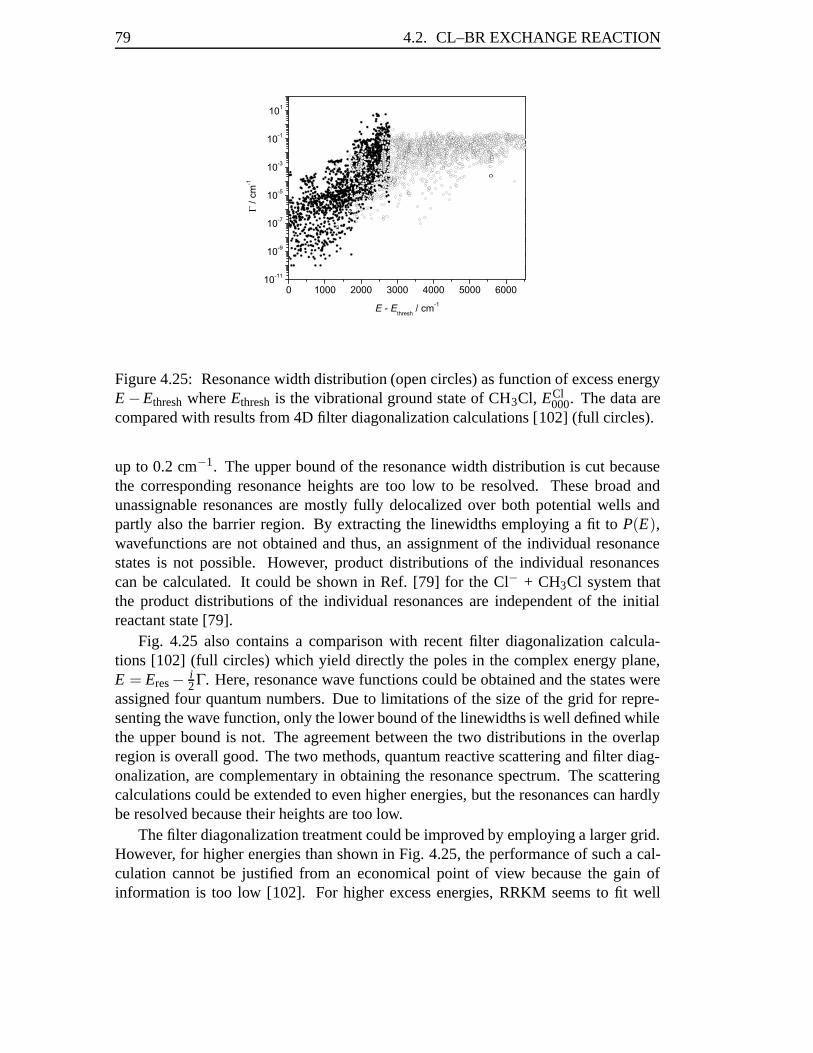
79 4.2. CL–BR EXCHANGE REACTION
Figure 4.25: Resonance width distribution (open circles) as function of excess energyE −Ethresh where Ethresh is the vibrational ground state of CH3Cl, ECl
000. The data arecompared with results from 4D filter diagonalization calculations [102] (full circles).
up to 0.2 cm−1. The upper bound of the resonance width distribution is cut becausethe corresponding resonance heights are too low to be resolved. These broad andunassignable resonances are mostly fully delocalized over both potential wells andpartly also the barrier region. By extracting the linewidths employing a fit to P(E),wavefunctions are not obtained and thus, an assignment of the individual resonancestates is not possible. However, product distributions of the individual resonancescan be calculated. It could be shown in Ref. [79] for the Cl− + CH3Cl system thatthe product distributions of the individual resonances are independent of the initialreactant state [79].
Fig. 4.25 also contains a comparison with recent filter diagonalization calcula-tions [102] (full circles) which yield directly the poles in the complex energy plane,E = Eres − i
2Γ. Here, resonance wave functions could be obtained and the states wereassigned four quantum numbers. Due to limitations of the size of the grid for repre-senting the wave function, only the lower bound of the linewidths is well defined whilethe upper bound is not. The agreement between the two distributions in the overlapregion is overall good. The two methods, quantum reactive scattering and filter diag-onalization, are complementary in obtaining the resonance spectrum. The scatteringcalculations could be extended to even higher energies, but the resonances can hardlybe resolved because their heights are too low.
The filter diagonalization treatment could be improved by employing a larger grid.However, for higher energies than shown in Fig. 4.25, the performance of such a cal-culation cannot be justified from an economical point of view because the gain ofinformation is too low [102]. For higher excess energies, RRKM seems to fit well
CHAPTER 4. RESULTS 80
while the performance of statistical theories for lower energies is only very poor [102].The number of resonances obtained from the scattering calculation is much smaller
than that resulting from filter diagonalization. For energies below the zero–point levelof CH3Br, only non–reactive processes Cl− + CH3Br (v′1,v
′2,v
′3) → Cl− + CH3Br
(v′′1,v′′2,v
′′3) are possible. In particular, for low energies with just a few open chan-
nels, every possible process exhibits a high background probability, which renders theextraction of resonances more difficult. In addition, some of these seem to show anon–Lorentzian behavior. Below the energy of the (0,0,1) state, only elastic scatter-ing is possible so that resonances cannot be computed from the squared moduli of theS–matrix elements.
4.2.4 Conclusions
(1) Time–independent quantum scattering calculations have been carried out onthe exothermic SN2 reaction Cl− + CH3Br → ClCH3 + Br− and the correspondingendothermic reverse reaction using hyperspherical coordinates describing the bondsbeing broken and formed. The two totally symmetric modes of the methyl group areincluded in the model. C3v symmetry is conserved throughout the reaction.
(2) A variant of the Lanczos scheme with a modified partial reorthogonalizationprocedure was formulated and employed in the calculations.
(3) A narrow grid in the total energy was employed so that long living resonancestates could be resolved. Resonances are extracted by fits to Lorentzian functions. Theresonance widths distribution provides a continuation of the data obtained by previousfilter diagonalization calculations. The agreement in the overlap region of the two datasets is good.
(4) While excitation of the umbrella bending mode already leads to a considerableenhancement of the reaction probability, its combination with vibrational excitation ofthe broken C–Br bond results in a strong synergic effect. This can be explained bythe similarity of the combined excitation with the classical transitional normal mode.Combination of C–Br stretch and C–H stretch does not show such a cooperative effect.
(5) Exciting the high–frequency symmetric C–H stretching vibration has a non–negligible effect on the reaction probability. For larger translational energies, however,the reaction probability for this mode initially excited follows the expected spectator–like behavior. The spectator concept is also questionable with respect to the productdistribution of states initially excited in the C–H stretch. Energy originally storedin this mode is released in other modes of the reaction products and by no meansconserved. Thus, the C–H stretch does not behave adiabatically, contrary to chemicalintuition and the expectation from the weak coupling to the other modes.
(6) In agreement with chemical intuition, excitation in the bond being broken leadsto higher reaction probabilities. However, if this mode contains too many quanta, theexpectation value of the bond becomes too large, i.e. the bond is overstretched andaway from the optimal geometry in the saddle point structure: The potential energyrises and the reactivity decreases.
81 4.3. RATE CONSTANTS IN THE CL–CL EXCHANGE REACTION
(7) Products are most likely formed in states with a high degree of excitation in thenewly formed bond. The internal modes of the methyl group are much less important.Reactants with combined umbrella/C–Br stretch excitation (one quantum each) mayyield products with two quanta in the umbrella mode. This high reactivity is onlyobserved for the combined initial state, not for pure bending excitation.
(8) In the endothermic reverse reaction, excitation of the symmetric C–H stretchingmode plays a very important role to overcome the barrier. Here, also initial stateswith two quanta in this mode could be considered. This energy is not even partly,i.e. yielding product states with one quantum in the C–H stretch, conserved, but isdistributed among the other modes, strongly contradicting the spectator mode concept.
(9) A comparison between the reactions of Cl− with CH3Cl and CH3Br, respec-tively, yields much higher probabilities for the latter case that are due to the absence ofa net barrier. Excitation of the umbrella mode, however, results in comparable reactionprobabilities. This effect is accidental and owing to the larger increase of reactivity inthe chlorine exchange reaction where the energy may be used to overcome the barrier.
(10) For low initial excitations, the product distributions of the endothermic reversereaction Br− + CH3Cl are similar to each other and also similar to those of the identityreaction Cl− + CH3Cl′ because the very narrow resonances decay independently oftheir formation.
4.3 Rate Constants in the Cl–Cl Exchange Reaction
4.3.1 Abstract
Within the framework of reduced–dimensionality quantum scattering theory, we em-ploy Bowman’s adiabatic rotation approximation to describe reactive systems that havesymmetric top geometries during the entire collision process. The results are com-pared with the approach of shifting the total energy by a characteristic rotational en-ergy. Initial–state selected and total thermal rate constants have been computed for thecomplex–forming gas–phase reaction Cl− + CH3Cl′ → ClCH3 + Cl′−. At room tem-perature, we find a significant contribution from energetically high vibrational modes.The dependence of the cross sections on the different angular momenta is analyzedin detail and high total angular momenta are found to be of considerable importance.The influence of adiabatic azimuthal rotation on the rate constants turns out to be smallcompared to other effects. In addition, we use a new model to account for the asym-metric modes not explicitly contained in the scattering calculations. The differenceto the only available experimental value confirms our conclusion that the Cl–C–Cl′bending modes are of major importance for this reaction.
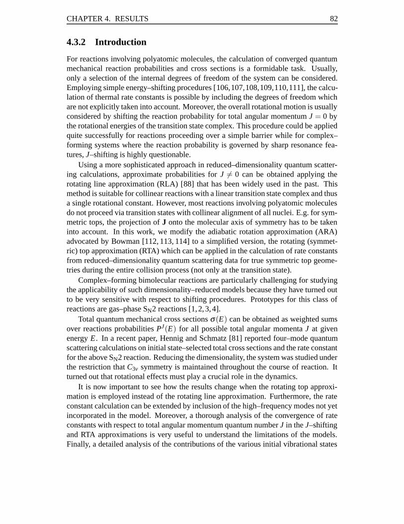
CHAPTER 4. RESULTS 82
4.3.2 Introduction
For reactions involving polyatomic molecules, the calculation of converged quantummechanical reaction probabilities and cross sections is a formidable task. Usually,only a selection of the internal degrees of freedom of the system can be considered.Employing simple energy–shifting procedures [106,107,108,109,110,111], the calcu-lation of thermal rate constants is possible by including the degrees of freedom whichare not explicitly taken into account. Moreover, the overall rotational motion is usuallyconsidered by shifting the reaction probability for total angular momentum J = 0 bythe rotational energies of the transition state complex. This procedure could be appliedquite successfully for reactions proceeding over a simple barrier while for complex–forming systems where the reaction probability is governed by sharp resonance fea-tures, J–shifting is highly questionable.
Using a more sophisticated approach in reduced–dimensionality quantum scatter-ing calculations, approximate probabilities for J �= 0 can be obtained applying therotating line approximation (RLA) [88] that has been widely used in the past. Thismethod is suitable for collinear reactions with a linear transition state complex and thusa single rotational constant. However, most reactions involving polyatomic moleculesdo not proceed via transition states with collinear alignment of all nuclei. E.g. for sym-metric tops, the projection of J onto the molecular axis of symmetry has to be takeninto account. In this work, we modify the adiabatic rotation approximation (ARA)advocated by Bowman [112, 113, 114] to a simplified version, the rotating (symmet-ric) top approximation (RTA) which can be applied in the calculation of rate constantsfrom reduced–dimensionality quantum scattering data for true symmetric top geome-tries during the entire collision process (not only at the transition state).
Complex–forming bimolecular reactions are particularly challenging for studyingthe applicability of such dimensionality–reduced models because they have turned outto be very sensitive with respect to shifting procedures. Prototypes for this class ofreactions are gas–phase SN2 reactions [1, 2, 3, 4].
Total quantum mechanical cross sections σ(E) can be obtained as weighted sumsover reactions probabilities PJ(E) for all possible total angular momenta J at givenenergy E. In a recent paper, Hennig and Schmatz [81] reported four–mode quantumscattering calculations on initial state–selected total cross sections and the rate constantfor the above SN2 reaction. Reducing the dimensionality, the system was studied underthe restriction that C3v symmetry is maintained throughout the course of reaction. Itturned out that rotational effects must play a crucial role in the dynamics.
It is now important to see how the results change when the rotating top approxi-mation is employed instead of the rotating line approximation. Furthermore, the rateconstant calculation can be extended by inclusion of the high–frequency modes not yetincorporated in the model. Moreover, a thorough analysis of the convergence of rateconstants with respect to total angular momentum quantum number J in the J–shiftingand RTA approximations is very useful to understand the limitations of the models.Finally, a detailed analysis of the contributions of the various initial vibrational states
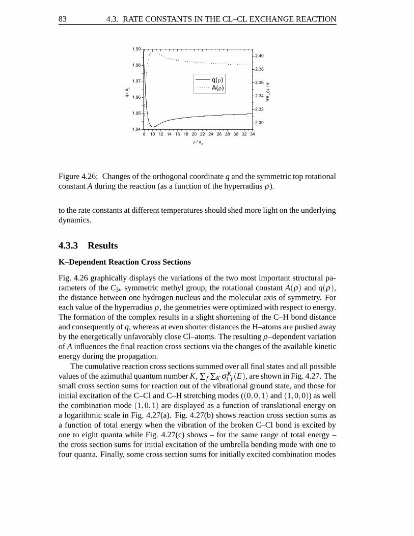
83 4.3. RATE CONSTANTS IN THE CL–CL EXCHANGE REACTION
Figure 4.26: Changes of the orthogonal coordinate q and the symmetric top rotationalconstant A during the reaction (as a function of the hyperradius ρ).
to the rate constants at different temperatures should shed more light on the underlyingdynamics.
4.3.3 Results
K–Dependent Reaction Cross Sections
Fig. 4.26 graphically displays the variations of the two most important structural pa-rameters of the C3v symmetric methyl group, the rotational constant A(ρ) and q(ρ),the distance between one hydrogen nucleus and the molecular axis of symmetry. Foreach value of the hyperradius ρ , the geometries were optimized with respect to energy.The formation of the complex results in a slight shortening of the C–H bond distanceand consequently of q, whereas at even shorter distances the H–atoms are pushed awayby the energetically unfavorably close Cl–atoms. The resulting ρ–dependent variationof A influences the final reaction cross sections via the changes of the available kineticenergy during the propagation.
The cumulative reaction cross sections summed over all final states and all possiblevalues of the azimuthal quantum number K, ∑ f ∑K σK
i, f (E), are shown in Fig. 4.27. Thesmall cross section sums for reaction out of the vibrational ground state, and those forinitial excitation of the C–Cl and C–H stretching modes ((0,0,1) and (1,0,0)) as wellthe combination mode (1,0,1) are displayed as a function of translational energy ona logarithmic scale in Fig. 4.27(a). Fig. 4.27(b) shows reaction cross section sums asa function of total energy when the vibration of the broken C–Cl bond is excited byone to eight quanta while Fig. 4.27(c) shows – for the same range of total energy –the cross section sums for initial excitation of the umbrella bending mode with one tofour quanta. Finally, some cross section sums for initially excited combination modes
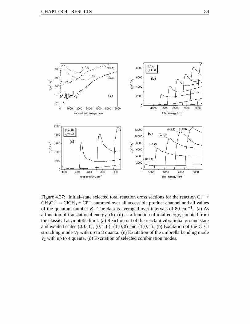
CHAPTER 4. RESULTS 84
Figure 4.27: Initial–state selected total reaction cross sections for the reaction Cl− +CH3Cl′ → ClCH3 + Cl′−, summed over all accessible product channel and all valuesof the quantum number K. The data is averaged over intervals of 80 cm−1. (a) Asa function of translational energy, (b)–(d) as a function of total energy, counted fromthe classical asymptotic limit. (a) Reaction out of the reactant vibrational ground stateand excited states (0,0,1), (0,1,0), (1,0,0) and (1,0,1). (b) Excitation of the C–Clstretching mode ν3 with up to 8 quanta. (c) Excitation of the umbrella bending modeν2 with up to 4 quanta. (d) Excitation of selected combination modes.
85 4.3. RATE CONSTANTS IN THE CL–CL EXCHANGE REACTION
Figure 4.28: Relative deviation of the state–selected cross section for initial state(0,0,0) for azimuthal quantum number K from the one for K − 1, weighted by thedifference of the squares of the azimuthal quantum numbers (see the text). Each crosssection is evaluated at the same translational energy E. The data is averaged over 600cm−1.
of C–Cl stretch and umbrella bend are displayed. The data can be compared to theK = 0 cross sections from Ref. [81]. Some of the differences are simply caused by thedifferent setting: In contrast to Ref. [81], the data in Fig. 4.27 has been averaged overintervals of 80 cm−1 resulting in less structure and acuteness. As we show cumulativecross sections summed over all K, the scale of the ordinates change by several orders ofmagnitude. However, some of the features in Fig. 4.27 could not be so easily predictedfrom our previous calculations: The envelope of the maxima becomes smoother; inFig. 4.27(b), the increase of the maxima has become much more monotonous (dipsat v3 = 3, 5 and 7 are missing). Also in Fig. 4.27(d), some curves change order withrespect to their maxima (e.g., (0,2,2) and (0,2,3)). For large values of the total energy,nearly all curves show a deviation from the 1/k2
i –behavior which is explained by thepresence of several of these prefactors due to the summation over different initial states(different K). Finally, in Fig. 4.27(a) the C–H-stretching mode does not reach thespectator mode regime valid for higher translational energies in contrast to Ref. [81]where such a spectator mode behavior can be observed within the displayed energyrange. We attribute this to the contribution of cross sections with higher K and thuslower translational energy.
In order to assess the influence of different values of K on the cross sections, weuse the quantity
σKi (E)−σK−1
i (E)(2K−1)σK−1
i (E)(4.7)
that gives the relative difference of these state–selected cross sections for K and K −1weighted by the difference of the squares of the azimuthal quantum numbers. In
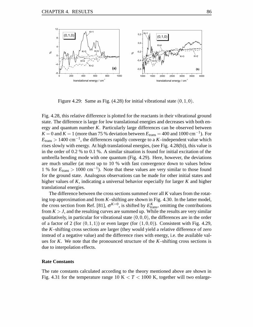
CHAPTER 4. RESULTS 86
Figure 4.29: Same as Fig. (4.28) for initial vibrational state (0,1,0).
Fig. 4.28, this relative difference is plotted for the reactants in their vibrational groundstate. The difference is large for low translational energies and decreases with both en-ergy and quantum number K. Particularly large differences can be observed betweenK = 0 and K = 1 (more than 75 % deviation between Etrans = 400 and 1000 cm−1). ForEtrans > 1400 cm−1, the differences rapidly converge to a K–independent value whichrises slowly with energy. At high translational energies, (see Fig. 4.28(b)), this value isin the order of 0.2 % to 0.1 %. A similar situation is found for initial excitation of theumbrella bending mode with one quantum (Fig. 4.29). Here, however, the deviationsare much smaller (at most up to 10 % with fast convergence down to values below1 % for Etrans > 1000 cm−1). Note that these values are very similar to those foundfor the ground state. Analogous observations can be made for other initial states andhigher values of K, indicating a universal behavior especially for larger K and highertranslational energies.
The difference between the cross sections summed over all K values from the rotat-ing top approximation and from K–shifting are shown in Fig. 4.30. In the latter model,the cross section from Ref. [81], σK=0, is shifted by EK
trans, omitting the contributionsfrom K > J, and the resulting curves are summed up. While the results are very similarqualitatively, in particular for vibrational state (0,0,0), the differences are in the orderof a factor of 2 (for (0,1,1)) or even larger (for (1,0,0)). Consistent with Fig. 4.29,the K–shifting cross sections are larger (they would yield a relative difference of zeroinstead of a negative value) and the difference rises with energy, i.e. the available val-ues for K. We note that the pronounced structure of the K–shifting cross sections isdue to interpolation effects.
Rate Constants
The rate constants calculated according to the theory mentioned above are shown inFig. 4.31 for the temperature range 10 K < T < 1000 K, together will two enlarge-
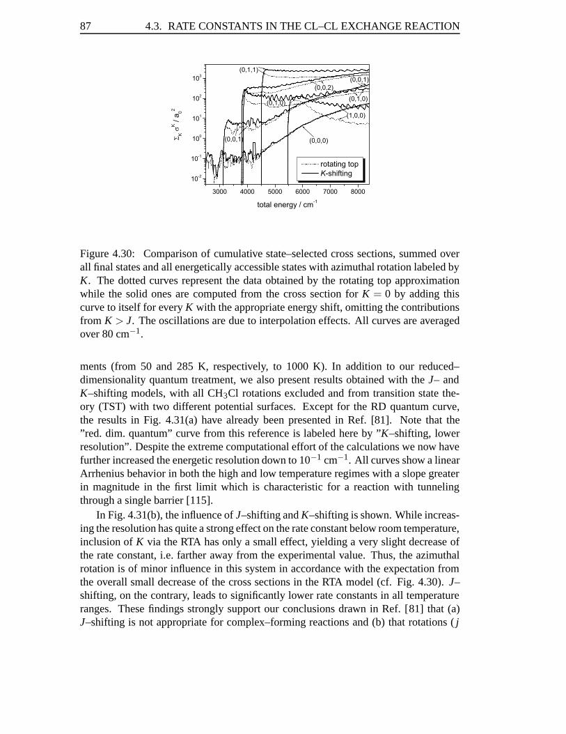
87 4.3. RATE CONSTANTS IN THE CL–CL EXCHANGE REACTION
Figure 4.30: Comparison of cumulative state–selected cross sections, summed overall final states and all energetically accessible states with azimuthal rotation labeled byK. The dotted curves represent the data obtained by the rotating top approximationwhile the solid ones are computed from the cross section for K = 0 by adding thiscurve to itself for every K with the appropriate energy shift, omitting the contributionsfrom K > J. The oscillations are due to interpolation effects. All curves are averagedover 80 cm−1.
ments (from 50 and 285 K, respectively, to 1000 K). In addition to our reduced–dimensionality quantum treatment, we also present results obtained with the J– andK–shifting models, with all CH3Cl rotations excluded and from transition state the-ory (TST) with two different potential surfaces. Except for the RD quantum curve,the results in Fig. 4.31(a) have already been presented in Ref. [81]. Note that the”red. dim. quantum” curve from this reference is labeled here by ”K–shifting, lowerresolution”. Despite the extreme computational effort of the calculations we now havefurther increased the energetic resolution down to 10−1 cm−1. All curves show a linearArrhenius behavior in both the high and low temperature regimes with a slope greaterin magnitude in the first limit which is characteristic for a reaction with tunnelingthrough a single barrier [115].
In Fig. 4.31(b), the influence of J–shifting and K–shifting is shown. While increas-ing the resolution has quite a strong effect on the rate constant below room temperature,inclusion of K via the RTA has only a small effect, yielding a very slight decrease ofthe rate constant, i.e. farther away from the experimental value. Thus, the azimuthalrotation is of minor influence in this system in accordance with the expectation fromthe overall small decrease of the cross sections in the RTA model (cf. Fig. 4.30). J–shifting, on the contrary, leads to significantly lower rate constants in all temperatureranges. These findings strongly support our conclusions drawn in Ref. [81] that (a)J–shifting is not appropriate for complex–forming reactions and (b) that rotations ( j
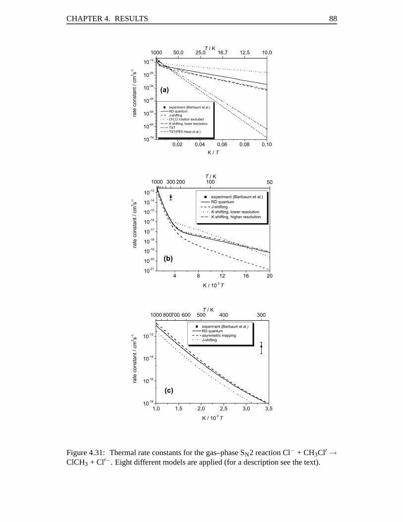
CHAPTER 4. RESULTS 88
Figure 4.31: Thermal rate constants for the gas–phase SN2 reaction Cl− + CH3Cl′ →ClCH3 + Cl′−. Eight different models are applied (for a description see the text).

89 4.3. RATE CONSTANTS IN THE CL–CL EXCHANGE REACTION
rotations of the reactant and product symmetric tops) play a crucial role in the system.For chemically relevant temperatures starting from 250 K, the results from K–shiftingand RTA are almost indistinguishable on the given scale and resolution effects becomenegligible.
It remains to study the influence of the asymmetric modes (i.e.,the higher–fre-quency doubly–degenerate C–H stretching and H–C–H bending modes) on the rateconstants (see Fig. 4.31(c)). We only present the combination with the RTA modeland observe a slight increase of k(T ) where this effect becomes somewhat more pro-nounced for higher temperatures. The effect is significantly smaller than that goingfrom J–shifting to RTA. Consequently, the asymmetric modes will have only a slighteffect on the rate constants within this temperature range as they are already expectedto be largely overestimated in the asymmetric mapping model [83] and thus their ex-plicit inclusion cannot explain the discrepancy to the experimental value. Note thatalso the symmetric modes do not yield the dominant contribution to the rate constant(cf. Fig. 4.32).
The influence of asymmetric modes compared to their symmetric counterparts hasbeen studied explicitly by several others. Wang and Bowman found the symmetricstretch of the H2O molecule in the OH+H2 → H+H2O reaction to be more popu-lated than the corresponding antisymmetric mode [116], whereas in the H+C2H2 →H2+C2H reaction the antisymmetric C–H stretch showed a higher effectivity to pro-mote the reaction [117]. In the O+CH4 → OH+CH3 reaction which is the most com-parable one to our investigations, calculations by Clary and Palma [86] resulted ina smaller reaction probability for the antisymmetric C–H stretch, but of comparablemagnitude. Experiments on the Cl + CH4 → HCl + CH3 reaction [118] show almostindistinguishable state–selected differential cross sections and rovibrational distribu-tions when the reactants are excited either in the symmetric or the antisymmetric C–Hstretching vibration. However, in all of these reactions the antisymmetric mode isintrinsically coupled to the reaction coordinate which is not the case for our reaction.
In Fig. 4.32, the contributions of the various initial vibrational states to the totalrate constant are analyzed in detail. The various curves show a linear Arrhenius be-havior within the selected temperature range and a lot of crossings; the ground stateitself exhibits two different slopes as does the total rate constant (with a different bridg-ing region, however), cf. Ref. [115]. This is very much different compared to non–complex–forming bimolecular reactions. A comparable system (however with lightatoms only), the abstraction reaction between a hydrogen atom and methane/methanol,was recently studied by Kerkeni and Clary with a state–selective analysis of the rateconstants [119, 120]. A direct comparison of the overall behavior is difficult becausethe higher barriers in these reactions cause the relevant interesting features to appear athigher, rarely investigated temperatures, and the smaller number of degrees of freedomconsidered yields less curves.
The relative contributions of the different initially excited vibrational states areshown in Fig. 4.32(b). The individual curves show a strikingly similar shape. Un-der thermal conditions, the state with two quanta in the C–Cl stretching mode of the
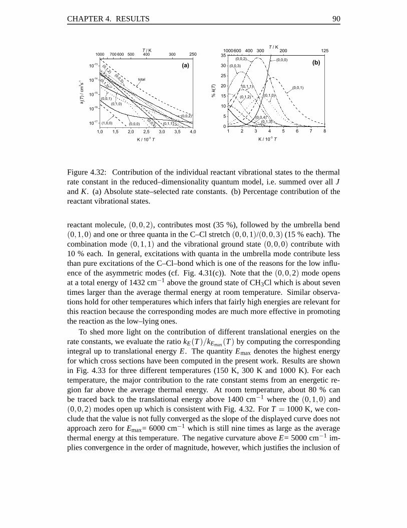
CHAPTER 4. RESULTS 90
Figure 4.32: Contribution of the individual reactant vibrational states to the thermalrate constant in the reduced–dimensionality quantum model, i.e. summed over all Jand K. (a) Absolute state–selected rate constants. (b) Percentage contribution of thereactant vibrational states.
reactant molecule, (0,0,2), contributes most (35 %), followed by the umbrella bend(0,1,0) and one or three quanta in the C–Cl stretch (0,0,1)/(0,0,3) (15 % each). Thecombination mode (0,1,1) and the vibrational ground state (0,0,0) contribute with10 % each. In general, excitations with quanta in the umbrella mode contribute lessthan pure excitations of the C–Cl–bond which is one of the reasons for the low influ-ence of the asymmetric modes (cf. Fig. 4.31(c)). Note that the (0,0,2) mode opensat a total energy of 1432 cm−1 above the ground state of CH3Cl which is about seventimes larger than the average thermal energy at room temperature. Similar observa-tions hold for other temperatures which infers that fairly high energies are relevant forthis reaction because the corresponding modes are much more effective in promotingthe reaction as the low–lying ones.
To shed more light on the contribution of different translational energies on therate constants, we evaluate the ratio kE(T )/kEmax(T ) by computing the correspondingintegral up to translational energy E. The quantity Emax denotes the highest energyfor which cross sections have been computed in the present work. Results are shownin Fig. 4.33 for three different temperatures (150 K, 300 K and 1000 K). For eachtemperature, the major contribution to the rate constant stems from an energetic re-gion far above the average thermal energy. At room temperature, about 80 % canbe traced back to the translational energy above 1400 cm−1 where the (0,1,0) and(0,0,2) modes open up which is consistent with Fig. 4.32. For T = 1000 K, we con-clude that the value is not fully converged as the slope of the displayed curve does notapproach zero for Emax= 6000 cm−1 which is still nine times as large as the averagethermal energy at this temperature. The negative curvature above E= 5000 cm−1 im-plies convergence in the order of magnitude, however, which justifies the inclusion of
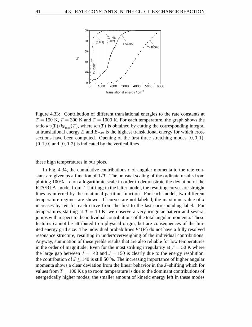
91 4.3. RATE CONSTANTS IN THE CL–CL EXCHANGE REACTION
Figure 4.33: Contribution of different translational energies to the rate constants atT = 150 K, T = 300 K and T = 1000 K. For each temperature, the graph shows theratio kE(T )/kEmax(T ), where kE(T ) is obtained by cutting the corresponding integralat translational energy E and Emax is the highest translational energy for which crosssections have been computed. Opening of the first three stretching modes (0,0,1),(0,1,0) and (0,0,2) is indicated by the vertical lines.
these high temperatures in our plots.
In Fig. 4.34, the cumulative contributions c of angular momenta to the rate con-stant are given as a function of 1/T . The unusual scaling of the ordinate results fromplotting 100%− c on a logarithmic scale in order to demonstrate the deviation of theRTA/RLA–model from J–shifting; in the latter model, the resulting curves are straightlines as inferred by the rotational partition function. For each model, two differenttemperature regimes are shown. If curves are not labeled, the maximum value of Jincreases by ten for each curve from the first to the last corresponding label. Fortemperatures starting at T = 10 K, we observe a very irregular pattern and severaljumps with respect to the individual contributions of the total angular momenta. Thesefeatures cannot be attributed to a physical origin, but are consequences of the lim-ited energy grid size: The individual probabilities PJ(E) do not have a fully resolvedresonance structure, resulting in under/overweighing of the individual contributions.Anyway, summation of these yields results that are also reliable for low temperaturesin the order of magnitude: Even for the most striking irregularity at T = 50 K wherethe large gap between J = 140 and J = 150 is clearly due to the energy resolution,the contribution of J ≤ 140 is still 50 %. The increasing importance of higher angularmomenta shows a clear deviation from the linear behavior in the J–shifting which forvalues from T = 100 K up to room temperature is due to the dominant contributions ofenergetically higher modes; the smaller amount of kinetic energy left in these modes

CHAPTER 4. RESULTS 92
Figure 4.34: Cumulative contribution c of angular momenta to the rate constant asa function of 1/T (see the text). (a) and (b) refer to J–shifting, whereas (c) and (d)contain the analogous data for the RTA/RLA–model.
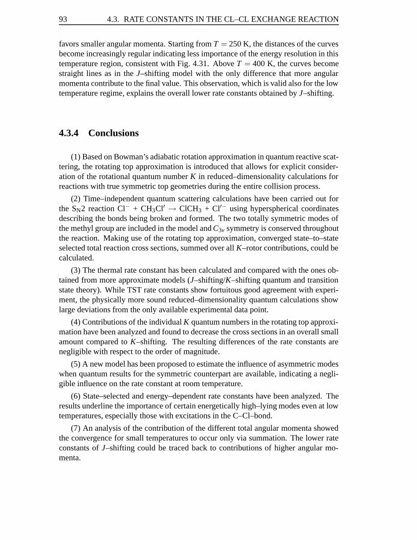
93 4.3. RATE CONSTANTS IN THE CL–CL EXCHANGE REACTION
favors smaller angular momenta. Starting from T = 250 K, the distances of the curvesbecome increasingly regular indicating less importance of the energy resolution in thistemperature region, consistent with Fig. 4.31. Above T = 400 K, the curves becomestraight lines as in the J–shifting model with the only difference that more angularmomenta contribute to the final value. This observation, which is valid also for the lowtemperature regime, explains the overall lower rate constants obtained by J–shifting.
4.3.4 Conclusions
(1) Based on Bowman’s adiabatic rotation approximation in quantum reactive scat-tering, the rotating top approximation is introduced that allows for explicit consider-ation of the rotational quantum number K in reduced–dimensionality calculations forreactions with true symmetric top geometries during the entire collision process.
(2) Time–independent quantum scattering calculations have been carried out forthe SN2 reaction Cl− + CH3Cl′ → ClCH3 + Cl′− using hyperspherical coordinatesdescribing the bonds being broken and formed. The two totally symmetric modes ofthe methyl group are included in the model and C3v symmetry is conserved throughoutthe reaction. Making use of the rotating top approximation, converged state–to–stateselected total reaction cross sections, summed over all K–rotor contributions, could becalculated.
(3) The thermal rate constant has been calculated and compared with the ones ob-tained from more approximate models (J–shifting/K–shifting quantum and transitionstate theory). While TST rate constants show fortuitous good agreement with experi-ment, the physically more sound reduced–dimensionality quantum calculations showlarge deviations from the only available experimental data point.
(4) Contributions of the individual K quantum numbers in the rotating top approxi-mation have been analyzed and found to decrease the cross sections in an overall smallamount compared to K–shifting. The resulting differences of the rate constants arenegligible with respect to the order of magnitude.
(5) A new model has been proposed to estimate the influence of asymmetric modeswhen quantum results for the symmetric counterpart are available, indicating a negli-gible influence on the rate constant at room temperature.
(6) State–selected and energy–dependent rate constants have been analyzed. Theresults underline the importance of certain energetically high–lying modes even at lowtemperatures, especially those with excitations in the C–Cl–bond.
(7) An analysis of the contribution of the different total angular momenta showedthe convergence for small temperatures to occur only via summation. The lower rateconstants of J–shifting could be traced back to contributions of higher angular mo-menta.
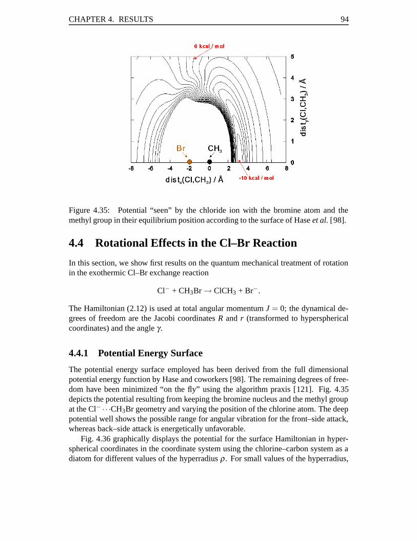
CHAPTER 4. RESULTS 94
Figure 4.35: Potential “seen” by the chloride ion with the bromine atom and themethyl group in their equilibrium position according to the surface of Hase et al. [98].
4.4 Rotational Effects in the Cl–Br Reaction
In this section, we show first results on the quantum mechanical treatment of rotationin the exothermic Cl–Br exchange reaction
Cl− + CH3Br → ClCH3 + Br−.
The Hamiltonian (2.12) is used at total angular momentum J = 0; the dynamical de-grees of freedom are the Jacobi coordinates R and r (transformed to hypersphericalcoordinates) and the angle γ .
4.4.1 Potential Energy Surface
The potential energy surface employed has been derived from the full dimensionalpotential energy function by Hase and coworkers [98]. The remaining degrees of free-dom have been minimized “on the fly” using the algorithm praxis [121]. Fig. 4.35depicts the potential resulting from keeping the bromine nucleus and the methyl groupat the Cl− · · ·CH3Br geometry and varying the position of the chlorine atom. The deeppotential well shows the possible range for angular vibration for the front–side attack,whereas back–side attack is energetically unfavorable.
Fig. 4.36 graphically displays the potential for the surface Hamiltonian in hyper-spherical coordinates in the coordinate system using the chlorine–carbon system as adiatom for different values of the hyperradius ρ . For small values of the hyperradius,
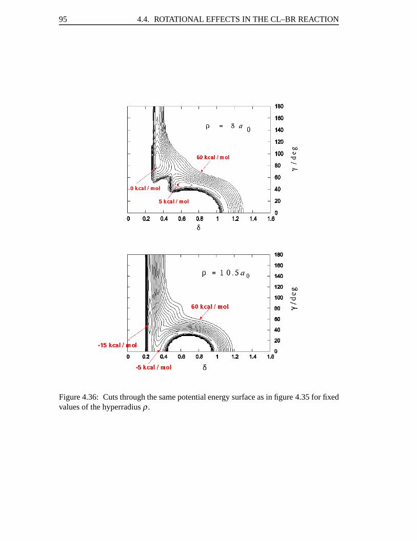
95 4.4. ROTATIONAL EFFECTS IN THE CL–BR REACTION
Figure 4.36: Cuts through the same potential energy surface as in figure 4.35 for fixedvalues of the hyperradius ρ .

CHAPTER 4. RESULTS 96

97 4.4. ROTATIONAL EFFECTS IN THE CL–BR REACTION
the equilibrium geometry is not collinear, but T–shaped. The situation changes withincreasing hyperradius. This gives rise to two different types of ground states depend-ing on the value of the reaction coordinate, and the crossing of these can clearly beseen in the hyperspherical adiabatic curves, Fig. 4.37. For asymptotic values of thehyperradius, the two reaction channels split. Owing to the nature of the coordinatespreferring one arrangement, the two asymptotic configurations give rise to completelydifferent shapes in the potential energy surface.
4.4.2 Numerical Details
We employed the Hamiltonian (2.12) in hyperspherical coordinates at total angularmomentum J = 0 with the chlorine–carbon entity treated as the diatom. The methodof R–matrix–propagation was used to compute the S–matrix. The surface Hamiltonianwas diagonalized at distances of dρ = 0.1 between ρmin = 6.5a0 and ρmax = 20.0a0,where in the last sector convergence was checked by recomputing the eigenstates in theother coordinate system (with the bromine–carbon entity treated as the diatom). Allchannels up to a total energy of Emax = 1500 cm−1 have been computed and includedin the R–matrix–propagation (with a maximum number of Nch,max = 1061 channels).No averaging of the final reaction probabilities w.r.t. ρ was used due to the rapidlychanging number of channels. The final S–matrix was computed at energy intervals ofΔE = 15 cm−1.
The basis for the matrix representation of the Hamiltonian was constructed by aPODVR (see Sec. 3.5) in both the hyperangle δ and the physical angle γ . For thelatter, the construction of the reference Hamiltonian needs some consideration as itcontains a rotational constant depending on the hyperangle δ :
Hrotref =
h2
2
(1
μρ2 cos2 δ+
1
μρ2 sin2 δ
)︸ ︷︷ ︸
:= B(δ )
j( j +1)+Vref(γ). (4.8)
We could have used a different constant B(δ (γ)) for each value of gamma; forexample, one could choose the hyperangle δ (γ) to be the value where V (γ,δ (γ)) =Vref(γ). This would lead to an operator that is not symmetric. It can easily be sym-metrized, but we found it nevertheless to be superior to use the minimum rotationalconstant Bmin := minδ PO B(δ PO) for all values of γ where δ PO denotes the collo-cation points in the hyperangle δ (the collocation basis in this coordinate needs tobe constructed first). Nδ = 1000 primitive sinc–collocation functions were used andNγ = 1400 Legendre polynomials for ρ ≤ 15.1a0; for 15.1a0 ≤ ρ ≤ 20a0, this numberwas increased to Nγ = 1900. The final sector–dependent potential optimized basis ineach coordinate was constructed from all corresponding collocation functions belowa certain energy. For the hyperangle δ , we set this energy Eδ
PO to EδPO = Emax +EPO
addwith EPO
add = 6000 cm−1; for the coordinate γ , the analogous quantity E γPO was com-

CHAPTER 4. RESULTS 98
Figure 4.37: Hyperspherical adiabatic curves. Shown is every tenth eigenvalue of thesurface Hamiltonian as a function of ρ .
puted from
EγPO = max
δ PO
Bmin
B(δ PO)(Eγ
ref−Vref(δ PO))+ +Vmin (4.9)
where Vref(δ ) is the minimum of the potential in the corresponding sector with thevalue δ of the hyperangle kept fixed, Vmin := minδ PO Vref(δ PO), Eγ
ref = EδPO in this
calculation and x+ := max(x,0) for any real number x.The cutoff energy Vcut was chosen to be Vcut = 21000 cm−1. The eigenvectors were
computed by the Lanczos algorithm with partial reorthogonalization (Sec. 3.6.2) usingthe convergence criterion (3.89) and ε = 10−6.
4.4.3 Results
Fig. 4.37 shows the hyperspherical adiabatic curves, where for clarity only a tenthof the eigenvalues has been included in the plot. The rapidly increasing density ofthe eigenstates with energy becomes apparent. An interesting feature is the crossingof the curves at ρ ≈ 11a0 due to the ground state changing to collinear geometry.Below that value, a non–collinear state will define the minimum energy configuration.Consequently, for small hyperradii ρ ≤ 8a0, a collinear treatment yields practicallyinfinite energies while inclusion of the coordinate γ provides lower eigenstates whichare finally T–shaped. In this way, we obtain an additional reaction mechanism withoutinversion of the methyl group (at still large energies, however).
Fig. 4.38 shows initial state–selected probabilities Pi(E) as functions of transla-tional energy Etrans. The curves are labeled with the initial number v of quanta in theC–Br stretching vibration and the angular quantum number j of the diatom (whichat this distances still corresponds to a vibration). Most striking is the increase of the

99 4.4. ROTATIONAL EFFECTS IN THE CL–BR REACTION
Figure 4.38: Initial state–selected probabilities Pi(E) as functions of translational en-ergy Etrans. The data is smoothed over intervals of 80 cm−1. Pi, f (E) is summed overall accessible product channels f .
reaction probability with the angular quantum number j. This points to an efficienttransfer of rotational energy to the reactive degrees of freedom, in agreement with ourconclusions from the previous sections.
To compare the collinear and three–dimensional results, Fig. 4.39 contains theinitial state–selected probabilities Pi(E) for two common states from the previouscollinear calculations, the ground state v = 0 and the first excited state of the C–Brstretching vibration v = 1. In addition, the states with v = 0 (with j = 0) and j = 9 (withv = 0) from the three–dimensional calculations have been included. While there is nosignificant enhancement of the reaction probability in the ground state, the situationis clearly different for the v = 1 state. The j = 9 already shows reaction probabilitiescomparable to those for the v = 1 state in the collinear calculations, clearly pointing tothe importance of this degree of freedom for the reaction. The larger variation of thethree–dimensional reaction probabilities is purely technical (due to a larger spacing ofthe points for which values have been obtained).
To obtain an estimate for the quality of the convergence of the data w.r.t. the hy-perradius ρ , Fig. 4.40 shows a comparison with reaction probabilities obtained bycomputing the S–matrix at ρ = 15.1a0 (where the wavefunctions in the two arrange-ment configurations already do not overlap). The clear enhancement of both the v = 0and the v = 1 probabilities can be attributed to the long range nature of the potentialand indicates the importance of evaluating the S–matrix at asymptotic regions of theconfiguration space. (This might be of some importance for the computation of rateconstants for high particle densities when the mean free path drops below the valuewhere the reactants can be considered free). In conjunction with established projec-

CHAPTER 4. RESULTS 100
Figure 4.39: Comparison of initial state–selected probabilities Pi(E) as functions oftranslational energy Etrans for a collinear calculation and the present one includingrotation. The data is smoothed over intervals of 80 cm−1. Pi, f (E) is summed over allaccessible product channels f .
Figure 4.40: Comparison of initial state–selected probabilities Pi(E) as functions oftranslational energy Etrans for evaluating the final S–matrix at ρ = 15.1a0 and ρ = 20a0.The data is smoothed over intervals of 80 cm−1. Pi, f (E) is summed over all accessibleproduct channels f .

101 4.4. ROTATIONAL EFFECTS IN THE CL–BR REACTION
tion techniques for the S–matrix, the algorithmic implementations in the present workopen up the window for such calculations.

Chapter 5
Summary and Outlook
In this thesis, the SN2 mechanism was investigated on a quantum mechanical level bymeans of time–independent scattering theory. Two model systems were considered,the thermoneutral chlorine–chlorine exchange reaction and the exothermic chlorine–bromine substitution.
For the first time, all degrees of freedom within C3v symmetry were treated exactlyin four–dimensional calculations. It could be shown that the umbrella bending motionand the C–H stretching vibration do not behave as spectator modes, but actively takepart in the reaction and enhance the reaction probability. Despite chemical intuition,the contrary is reported for the umbrella bending motion in the literature. For the C–Hstretching vibration, this effect could be traced back to long–lived resonances duringthe formation of the complex in comparison with filter–diagonalization studies. By aspecific algorithm, resonance linewidths were obtained in the scattering calculationswhich varied over ten orders of magnitude. For the carbon–halogen stretching vibra-tion, a saturation effect was observed which could be explained by an overstretchingof the bond beyond the optimal transition state geometry. Simultaneous excitation ofthe carbon–halogen stretching vibration and the umbrella bending motion resulted in astrong increase of the reaction probability due to the correspondence of this excitationto the transitional normal mode.
A detailed analysis of the cross sections and rate constants has been carried out.Different levels of approximation for the angular momenta involved and the remain-ing vibrational degrees of freedom have been investigated, using a new model forthe asymmetric vibrations of the methyl group. State–selective analysis of the rateconstants confirmed our conclusions about the influence of the symmetric vibrationalmodes in the SN2 process. Comparison with experimental data indicated that the ro-tation of the attacked methyl halide should be investigated on a quantum mechanicallevel as could be already inferred from trajectory calculations.
For that purpose, algorithms for a spatially three–dimensional treatment of an SN2reaction have been developed. While in the literature there is an abundance of resultsfor light three–atom systems with short range potentials, starting with collinear mod-els on H+H2 [122,123] to a state–selective comparison of theoretical and experimental

CHAPTER 5. SUMMARY AND OUTLOOK 104
differential cross sections [124], the present work represents the first investigation ofrotational effects in a heavy six–atom system with long–range interaction potentials ona quantum mechanical time–independent level. The results point indeed to an enhance-ment of the reaction probability with an excitation of the angular degree of freedom.Computations of state–selective differential cross sections are now within reach and to-gether with promising advances in the experimental setup [125] a better understandingof the SN2 mechanism becomes feasible.

Acknowledgements
It is a pleasure for me to thank Stefan Schmatz for the introduction to the interestingfield of reaction dynamics and the close and fruitful cooperation during the last years.
I would also like to thank Peter Botschwina for the opportunity to perform thisresearch, Rainer Oswald for his constant and professional support in all kinds of com-puter problems, Volker Dyczmons for the good working atmosphere and Denis Yalalovfor providing assistance in bridging the gap to organic chemistry.
Furthermore, I benefited from stimulating discussions with Markus Reiher on di-agonalization techniques and with Roland Wester on the link between experimentaland theoretical results in this field.
Financial support from the DFG through grants 1651/1-1 as well as 1651/1-2and the graduate school 782 (Spectroscopy and Dynamics of Molecular Aggregates,Chains and Coils) is gratefully acknowledged. Computing time was provided bythe John von Neumann–Institut for Computing (Julich) and the Gesellschaft fur wis-senschaftliche Datenverarbeitung mbH Gottingen.
Finally, I especially thank my parents and my brother for their continuous supportand encouragement during this thesis.

Bibliography
[1] W. L. Hase, Science 266, 998 (1994).
[2] M. L. Chabinyc, S. L. Craig, C. K. Regan and J. I. Brauman, Science 279, 1882(1998).
[3] J. K. Laerdahl and E. Uggerud, Int. J. Mass Spectrom. Ion Proc. 214, 277 (2002).
[4] S. Schmatz, Chem. Phys. Chem. 5, 600 (2004).
[5] Retrieved December 8, 2005, from Wikipedia, The Free Encyclopedia, onthe World Wide Web: http://de.wikipedia.org/wiki/Bild:Adrenalin3d.PNG andhttp://de.wikipedia.org/wiki/Bild:Biosynthese Adrenalin.png
[6] C. L. Gee, J. D. A. Tyndall, G. L. Grunewald, Q. Wu, M. J. McLeish and J. L. Mar-tin, Biochemistry 44, 16875 (2005).
[7] W. N. Olmstaed and J. I. Brauman, J. Am. Chem. Soc. 99, 4219 (1977).
[8] J. A. Dodd and J. I. Brauman, J. Phys. Chem. 90, 3559 (1986).
[9] J. I. Brauman, J. Mass Spectrom. 30, 1649 (1995).
[10] S. E. Barlow, J. M. VanDoren and V. M. Bierbaum, J. Am. Chem. Soc. 110, 7240(1988).
[11] S. Kato, G. E. Davico, H. S. Lee, C. H. Depuy and V. M. Bierbaum,Int. J. Mass Spectrom. 210/211, 223 (2001).
[12] A. A. Viggiano, R. A. Morris, J. S. Paschkewitz and J. F. Paulson,J. Am. Chem. Soc. 114, 10477 (1992).
[13] J.-L. Le Garrec, B. R. Rowe, J. L. Queffelec, J. B. A. Mitchell and D. C. Clary,J. Phys. Chem. 107, 1021 (1997).
[14] V. F. DeTuri, P. A. Hintz and K. M. Ervin, J. Phys. Chem. 101, 5969 (1997).
[15] K. M. Ervin, Int. J. Mass Spectrom. 187, 343 (1999).

BIBLIOGRAPHY 108
[16] L. A. Angel and K. M. Ervin, J. Phys. Chem. A 105, 4042 (2001).
[17] L. A. Angel, S. P. Garcia and K. M. Ervin, J. Am. Chem. Soc. 124, 336 (2002).
[18] L. A. Angel and K. M. Ervin, J. Am. Chem. Soc. 125, 1014 (2003).
[19] R. Wester, A. E. Bragg, A. V. Davis and D. M. Neumark, J. Chem. Phys. 119,10032 (2003).
[20] S. R. Vande Linde and W. L. Hase, J. Chem. Phys. 93, 7962 (1990).
[21] Y. J. Cho, S. R. Vande Linde, L. Zhu and W. R. Hase, J. Chem. Phys. 96, 8275(1992).
[22] W. L. Hase and Y. J. Cho, J. Chem. Phys. 98, 8626 (1993).
[23] G. H. Peslherbe, H. Wang and W. L. Hase, J. Chem. Phys. 102, 5626 (1995).
[24] G. H. Peslherbe, H. Wang and W. L. Hase, J. Am. Chem. Soc. 118, 257 (1996).
[25] D. J. Mann and W. L. Hase, J. Phys. Chem. A 102, 6208 (1998).
[26] T. Su and W. L. Hase, J. Phys. Chem. A 102, 9819 (1998).
[27] G. S. Li and W. L. Hase, J. Am. Chem. Soc. 121, 7124 (1999).
[28] K. Y. Song, L. P. Sun and W. L. Hase, J. Am. Chem. Soc. 123, 5753 (2001).
[29] S. C. Tucker and D. G. Truhlar, Chem. Phys. Lett. 157, 164 (1989).
[30] Y. Wang, W. L. Hase and H. Wang, J. Chem. Phys. 118, 2688 (2003).
[31] S. Schmatz and D. C. Clary, J. Chem. Phys. 110, 9483 (1999).
[32] S. Schmatz, P. Botschwina, J. Hauschildt and R. Schinke, J. Chem. Phys. 117,9710 (2002).
[33] J. Makarewicz, J. Phys. B: At. Mol. Opt. Phys. 21, 1803 (1987).
[34] J. R. Henderson, S. Miller and J. Tennyson, J. Chem. Soc. Faraday Trans. 86,1963 (1990).
[35] G. C. Schatz, Chem. Phys. Lett. 150, 92 (1988).
[36] D. C. Clary, J. Chem. Phys. 95, 7298 (1991).
[37] J. Echave and D. C. Clary, J. Chem. Phys. 100, 402 (1994).
[38] S. K. Pogrebnya, J. Echave and D. C. Clary, J. Chem. Phys. 107, 8975 (1997).
109 BIBLIOGRAPHY
[39] A. Kuppermann, J. A. Kaye and J. P. Dwyer, Chem. Phys. Lett. 74, 257 (1980).
[40] J. Romelt, Chem. Phys. Lett. 74, 263 (1980).
[41] B. Podolsky Phys. Rev. 32, 812 (1918).
[42] F. T. Smith, Phys. Rev. 118, 349 (1960).
[43] M. S. Child, Molecular Collision Theory (Dover, New York, 1996).
[44] R. T. Pack and G. A. Parker, J. Chem. Phys. 87, 3888 (1987).
[45] K. Museth and A. Kuppermann, J. Chem. Phys. 115, 8285 (2001).
[46] E. B. Stechel, R. B. Walker and J. C. Light, J. Chem. Phys. 69, 3518 (1978).
[47] C. Canuto, M. Y. Hussaini, A. Quarteroni and T. A. Zang, Spectral Methods inFluid Dynamics (Springer Verlag, New York, 1988).
[48] R. N. Ashcroft, Asset Pricing with Spectral Methods, (Stanford, PhD Thesis,1995).
[49] D. O. Harris, G. G. Engerholm and W. D. Gwinn, J. Chem. Phys. 43, 1515 (1965).
[50] A. S. Dickinson and P. R. Certain, J. Chem. Phys. 49, 4209 (1968).
[51] H. Wilf, In Mathematics for the Physical Sciences (John Wiley & Sons, Inc., NewYork, 1962), Chapter 2.
[52] J. Echave and D. C. Clary, Chem. Phys. Lett. 190, 225 (1992).
[53] D. T. Colbert and W. H. Miller, J. Chem. Phys. 96, 1982 (1992).
[54] G. C. Groenenboom and D. T. Colbert, J. Chem. Phys. 99, 9681 (1993).
[55] G. H. Golub and J. Welsch, Math. Comp. 23, 221 (1969).
[56] W. Gautschi, Math. Comp. 24, 245 (1970).
[57] D. Baye and P. H. Heenen, J. Phys. A: Math. Gen. 19, 2041 (1986).
[58] R. G. Littlejohn and P. Wright, J. Math. Phys. 43, 4668 (2002).
[59] V. Szalay, G. Czako, A. Nagy, T. Furtenbacher and A. G. Csazar, J. Chem. Phys.119, 10512 (2003).
[60] J. C. Light and T. Carrington Jr., Adv. Chem. Phys. 114, 263 (2000).
[61] N. L. Carothers, A Short Course on Approximation Theory (Lecture Notes, De-partment of Mathematics and Statistics, Bowling Green State University, 1998).

BIBLIOGRAPHY 110
[62] M. J. Bramley and T. Carrington Jr., J. Chem. Phys. 99, 8519 (1993).
[63] J. P. Boyd, Chebyshev and Fourier Spectral Methods (Second Edition, Dover,New York, 2001).
[64] R. Jaquet, Comput. Phys. Commun. 58, 257 (1990).
[65] A. G. Abrashkevich, D. G. Abrashkevich, M. S. Kashiev and I. V. Puzynin, Com-put. Phys. Commun. 85, 40 (1995).
[66] H. Wei, J. Chem. Phys. 106, 6885 (1997).
[67] R. G. Littlejohn, M. Cargo, T. Carrington Jr., K. A. Mitchell and B. Poirer,J. Chem. Phys. 116, 8691 (2002).
[68] J. C. Light, I. P. Hamilton and J. V. Lill, J. Chem. Phys. 82, 1400 (1984).
[69] R. B. Lehoucq, D. C. Sorensen and C. Yang, ARPACK Users’ Guide: Solutionof Large–Scale Eigenvalue Problems with Implicitly Restarted Arnoldi Methods(SIAM, Philadelphia, 1998).
[70] Z. Bai and R. Li, In Templates for the Solution of Algebraic Eigenvalue Prob-lems; D. Bai, J. Demmel, J. Dongarra, A. Ruhe, H. von der Vorst, Ed. (SIAM,Philadelphia, 2000), p. 106.
[71] C. Davis and W. Kahan, III. SIAM J. Numer. Anal. 7, 1 (1970).
[72] G. W. Stewart and J. G. Sun, Matrix Pertubation Theory (Academic Press, NewYork, 1990).
[73] C. Lanczos, J. Res. Natl. Bur. Stand. 45, 255 (1950).
[74] H. D. Simon, Math. Comput. 42, 115 (1984).
[75] H. G. Yu, G. Nyman, Chem. Phys. Lett. 298, 27 (1998).
[76] G. L. G. Sleijpen and H. A. van der Vorst, SIAM J. Matrix Anal. Appl. 17, 401(1996).
[77] E. R. Davidson, J. Comput. Phys. 17, 87 (1975).
[78] C. C. Page and M. A. Saunders, SIAM J. Numer. Anal. 12, 617 (1975).
[79] C. Hennig and S. Schmatz, J. Chem. Phys. 121, 220 (2004).
[80] P. Botschwina, C. Hennig and S. Schmatz, Phys. Chem. Chem. Phys. 6, 4630(2004).
[81] C. Hennig and S. Schmatz, Phys. Chem. Chem. Phys. 7, 1552 (2005).
111 BIBLIOGRAPHY
[82] C. Hennig and S. Schmatz, J. Chem. Phys. 122, no. 234307 (2005).
[83] C. Hennig and S. Schmatz, J. Phys. Chem. A 110, 1524 (2006).
[84] C. Hennig, R. B. Oswald and S. Schmatz, J. Phys. Chem. A 110, 3071 (2006).
[85] J. Palma and D. C. Clary, J. Chem. Phys. 112, 1859 (2000).
[86] J. Palma and D. C. Clary, Phys. Chem. Chem. Phys. 2, 4105 (2000).
[87] H. G. Yu and G. Nyman, J. Chem. Phys. 112, 238 (2000).
[88] M. S. Child, Mol. Phys. 12, 401 (1967).
[89] S. Schmatz and D. C. Clary, J. Chem. Phys. 109, 8200 (1998).
[90] M. I. Hernandez, J. Campos-Martinez, P. Villarreal, S. Schmatz, and D. C. Clary,Phys. Chem. Chem. Phys. 1, 1197 (1999).
[91] D. C. Clary and J. Palma, J. Chem. Phys. 106, 575 (1997).
[92] H. G. Yu and G. Nyman, Chem. Phys. Lett. 312, 585 (1999).
[93] S. Schmatz, P. Botschwina, J. Hauschildt and R. Schinke, J. Chem. Phys. 114,5233 (2001).
[94] S. Schmatz and J. Hauschildt, J. Chem. Phys. 118, 4499 (2003).
[95] J. L. Duncan and M. M. Law, J. Mol. Spectrosc. 140, 13 (1990).
[96] S. Schmatz, Chem. Phys. Lett. 330, 188 (2000).
[97] S. R. Vande Linde and W. L. Hase, J. Phys. Chem. 94, 2778 (1990).
[98] H. Wang, L. Zhu and W. L. Hase, J. Phys. Chem. 98, 1608 (1994).
[99] H. Zhang and S. C. Smith, J. Chem. Phys. 115, 5751 (2001).
[100] H. Wang, E. M. Goldfield and W. L. Hase, J. Chem. Soc. Faraday Trans. 93,737 (1997).
[101] S. Schmatz, H. Stoll and P. Botschwina, Int. J. Mass Spectr. Ion Proc. 291, 277(2000).
[102] S. Schmatz, J. Chem. Phys. 122, no. 234306 (2005).
[103] S. T. Graul and M. T. Bowers, J. Am. Chem. Soc. 113, 9696 (1991).
[104] S. T. Graul and M. T. Bowers, J. Am. Chem. Soc. 116, 3875 (1994).
BIBLIOGRAPHY 112
[105] G. Herzberg, Molecular Spectra and Molecular Structure. II. Infrared and Ra-man Spectra of Polyatomic Molecules (Van Nostrand Reinhold, New York, 1945).
[106] J. M. Bowman, Adv. Chem. Phys. 65, 61 (1985).
[107] J. M. Bowman and A. F. Wagner, In The Theory of Chemical Reaction Dynam-ics; D. C. Clary, Ed. (Reidel: Dordrecht, 1986), p. 47.
[108] R. B. Walker and E. F. Hayes, In The Theory of Chemical Reaction Dynamics;D. C. Clary, Ed. (Reidel: Dordrecht, 1986), p. 105.
[109] J. M. Bowman, J. Chem. Phys. 95, 4960 (1991).
[110] J. M. Bowman and D. Wang, In Advances in Molecular Vibration and CollisionDynamics; J. M. Bowman, Ed. (JAI, Greenwich, 1994, Vol. II B), p. 187.
[111] F. N. Dzegilenko and J. M. Bowman, J. Chem. Phys. 105, 2280 (1996).
[112] J. M. Bowman, Chem. Phys. Lett. 217, 36 (1994).
[113] J. M. Bowman, J. Phys. Chem. A 102, 3006 (1998).
[114] J. M. Bowman, Theor. Chem. Acc. 108, 125 (2002).
[115] R. P. Bell, Proc. R. Soc. A 139, 466 (1933).
[116] D. Wang, and J. M. Bowman, J. Chem. Phys. 96, 8906 (1992).
[117] D. Wang and J. M. Bowman, J. Chem. Phys. 101, 8646 (1994).
[118] H. A. Bechtel, J. P. Camden, D. J. Ankeny Brown and R. N. Zare, J. Chem. Phys.120, 5096 (2004).
[119] B. Kerkeni and D. C. Clary, J. Chem. Phys. 120, 2308 (2004).
[120] B. Kerkeni and D. C. Clary, J. Chem. Phys. 121, 6809 (2004).
[121] R. P. Brent, Algorithms for Minimization without Derivatives (Prentice–Hall,1973); program available from a.cs.okstate.edu in the /pub/jpc directory.
[122] E. M. Mortensen and K. S. Pitzer, Chem. Soc. (London), Spec. Publ. 16, 57(1962).
[123] D. G. Truhlar and A. Kuppermann, J. Chem. Phys. 52, 3841 (1970).
[124] S. D. Chao, S. A. Harich, D. X. Dai, C. C. Wang, X. Yang and R. T. Skodje,J. Chem. Phys. 117, 8341 (2002).
[125] J. Mikosch, U. Fruhling, S. Trippel, D. Schwalm, M. Weidemuller andR. Wester, Phys. Chem. Chem. Phys. 8, 2990 (2006).

Lebenslauf
Dipl.–Phys. Carsten Hennig, M.S. (USA)geboren am 17.4.1974 in HamburgStaatsangehorigkeit: deutsch
09/1980 – 06/1993 Schulbesuch in Isernhagen; Abitur
10/1993 – 09/1994 Wehrdienst
10/1994 – 07/1999 Studium der Physik und der Mathematik an der Uni-versitat Gottingen
07/1996 Vordiplom in Mathematik
10/1996 Vordiplom in Physik
07/1997 – 10/2000 Stipendiat der Studienstiftung des deutschen Volkes
07/1999 Diplom in Physik mit einer Diplomarbeit in theoreti-scher Physik
08/1999 – 07/2000 Mathematikstudium an der Michigan State University(USA); Master of Science in Mathematics
10/2000 – 06/2002 Wissenschaftlicher Mitarbeiter an der UniversitatGottingen
seit 10/2002 Doktorand in theoretischer Chemie an der UniversitatGottingen