augmented dickey-fuller test equation dependent variable: d(lgdpi) method: least squares sample...

Augmented Dickey-Fuller Test Equation Dependent Variable: D(LGDPI) Method: Least Squares Sample (adjusted): 1960 2003 Included observations: 44 after adjustments ============================================================ Variable Coefficient Std. Error t-Statistic Prob. ============================================================ LGDPI(-1) -0.090691 0.050826 -1.784362 0.0818 C 0.723299 0.381112 1.897865 0.0648 @TREND(1959) 0.002622 0.001705 1.537390 0.1319 ============================================================R-squared 0.164989 Mean dependent var 0.034225 Adjusted R-squared 0.124257 S.D. dependent var 0.016388 S.E. of regression 0.015336 Akaike info criter-5.451443 Sum squared resid 0.009643 Schwarz criterion -5.329794 Log likelihood 122.9317 Hannan-Quinn crite-5.406330 F-statistic 4.050580 Durbin-Watson stat 1.776237 Prob(F-statistic) 0.024814 ============================================================

TESTS OF NONSTATIONARITY: EXAMPLE AND FURTHER COMPLICATIONS

1

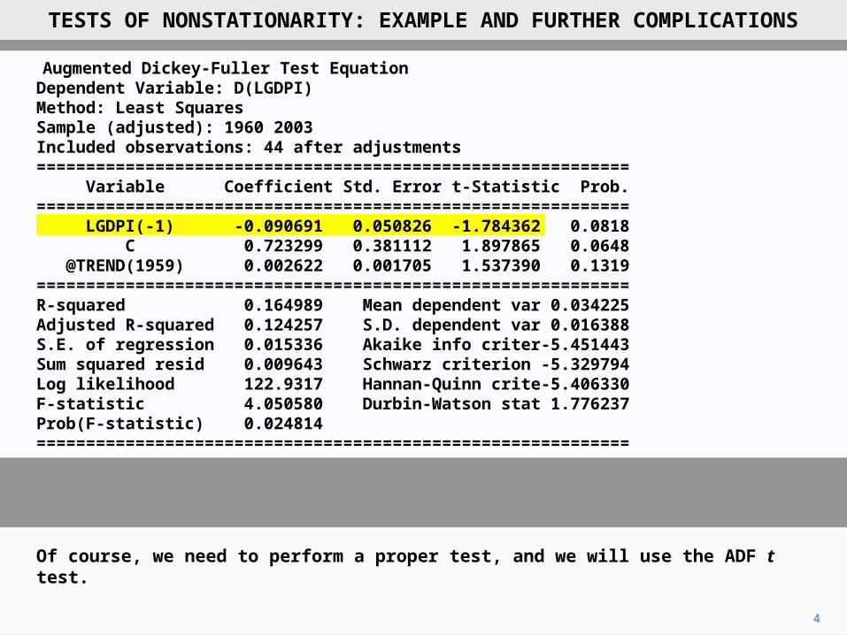
The table shows the second half of the EViews output when performing an ADF test on the logarithm of DPI. The value of p has been determined by the BIC (SIC) and turns out to be zero, so the regression is of the change of log income on lagged log income and time.

2

The time trend has been included because and inspection of the data reveals that the process is strongly trended and that therefore we need to discriminate between Case (c) (a random walk with drift) and Case (d) (a deterministic trend).



3

The coefficient of LGDPIt–1 is –0.09, close to zero. The null hypothesis is that the process is nonstationary. Under H0: the true value of the coefficient of LGDPIt–1 would be zero. So the near-zero coefficient suggests that the process is nonstationary.



4

Of course, we need to perform a proper test, and we will use the ADF t test.



Augmented Dickey-Fuller Unit Root Test on LGDPI============================================================Null Hypothesis: LGDPI has a unit root Exogenous: Constant, Linear Trend Lag Length: 0 (Automatic based on SIC, MAXLAG=9) ============================================================ t-Statistic Prob.* ============================================================Augmented Dickey-Fuller test statistic -1.784362 0.6953 Test critical values1% level -4.180911 5% level -3.515523 10% level -3.188259 ============================================================*MacKinnon (1996) one-sided p-values.

============================================================ Variable Coefficient Std. Error t-Statistic Prob. ============================================================ LGDPI(-1) -0.090691 0.050826 -1.784362 0.0818 C 0.723299 0.381112 1.897865 0.0648 @TREND(1959) 0.002622 0.001705 1.537390 0.1319 ============================================================

5

The t statistic, reproduced at the top of the output where it is designated the ADF test statistic, is –1.78.


6

Under the null hypothesis of nonstationarity, the critical value of t at the 5 percent level, also given at the top of the output, is –3.52, and hence the null hypothesis of nonstationarity is not rejected.




7

Notice that the critical value is much larger than 1.69, the conventional critical value for a one-sided test at the 5 percent level for a sample of this size.




Augmented Dickey-Fuller Test Equation Dependent Variable: D(LGDPI,2) Method: Least Squares Sample (adjusted): 1961 2003 Included observations: 43 after adjustments ============================================================ Variable Coefficient Std. Error t-Statistic Prob. ============================================================ D(LGDPI(-1)) -0.817536 0.153932 -5.311020 0.0000 C 0.028136 0.005872 4.791700 0.0000 ============================================================R-squared 0.407574 Mean dependent var-6.15E-05 Adjusted R-squared 0.393124 S.D. dependent var 0.021111 S.E. of regression 0.016446 Akaike info criter-5.332042 Sum squared resid 0.011090 Schwarz criterion -5.250126 Log likelihood 116.6389 Hannan-Quinn crite-5.301834 F-statistic 28.20694 Durbin-Watson stat 2.035001 Prob(F-statistic) 0.000004 ============================================================

8

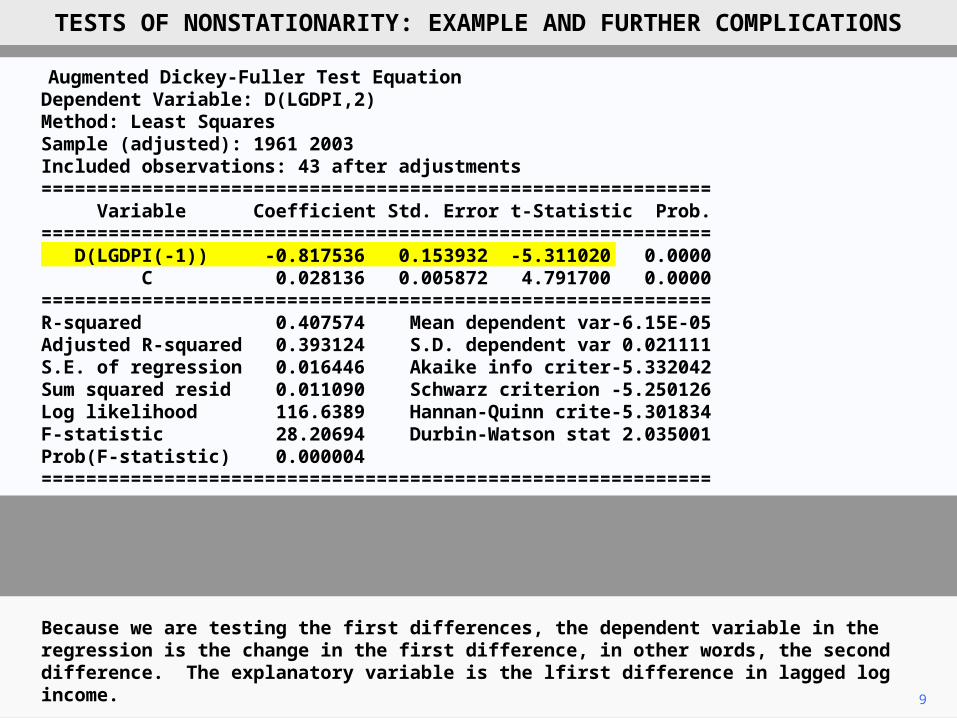
We now take first differences of the data for log income and again test for nonstationarity. An inspection of the differenced series reveals no trend, so we need to discriminate between Case (a) (a stationary process) and Case (b) (a random walk). We do not need to consider a time trend.


9

Because we are testing the first differences, the dependent variable in the regression is the change in the first difference, in other words, the second difference. The explanatory variable is the lfirst difference in lagged log income.



10

The table shows the second half of the EViews output when performing an ADF test on the differenced series. The coefficient of DLGDPIt–1 is –0.82, well below zero, suggesting that the null hypothesis of a nonstationary process should be rejected.



Augmented Dickey-Fuller Unit Root Test on D(LGDPI)============================================================Null Hypothesis: D(LGDPI) has a unit root Exogenous: Constant Lag Length: 0 (Automatic based on SIC, MAXLAG=9) ============================================================ t-Statistic Prob.* ============================================================Augmented Dickey-Fuller test statistic -5.311020 0.0001 Test critical values1% level -3.592462 5% level -2.931404 10% level -2.603944 ============================================================*MacKinnon (1996) one-sided p-values. ============================================================ Variable Coefficient Std. Error t-Statistic Prob. ============================================================ D(LGDPI(-1)) -0.817536 0.153932 -5.311020 0.0000 C 0.028136 0.005872 4.791700 0.0000 ============================================================

11

This is confirmed by the t statistic, –5.31, which allows the null hypothesis of nonstationarity to be rejected at the 1 percent level (critical value –3.59).


Augmented Dickey-Fuller Unit Root Test on D(LGDPI)============================================================Null Hypothesis: D(LGDPI) has a unit root Exogenous: Constant Lag Length: 0 (Automatic based on SIC, MAXLAG=9) ============================================================ t-Statistic Prob.* ============================================================Augmented Dickey-Fuller test statistic -5.311020 0.0001 Test critical values1% level -3.592462 5% level -2.931404 10% level -2.603944 ============================================================*MacKinnon (1996) one-sided p-values. ============================================================ Variable Coefficient Std. Error t-Statistic Prob. ============================================================ D(LGDPI(-1)) -0.817536 0.153932 -5.311020 0.0000 C 0.028136 0.005872 4.791700 0.0000 ============================================================

12

The tests therefore suggest that the logarithm of DPI is generated as an I(1) process. ADF–GLS tests produce very similar results for both levels and first differences.


13


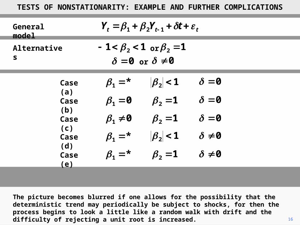
The previous slideshows may have suggested that discriminating between the possible cases is straightforward, apart from indeterminacy caused by the lower power of the tests. However, there are further issues.

ttt tYY 121

11 2 12 0 0

or

or

12 0

12 01 0

12 01 0

12 0

*1

*1

12 0*1

General model

Alternatives

Case (a)

Case (b)

Case (c)

Case (d)

Case (e)

14

If a process obviously possesses a trend, it should be possible to discriminate between the null hypothesis of a unit root and the alternative hypothesis of a deterministic trend, despite the low power of the tests that have been proposed, if one has enough observations.


ttt tYY 121

11 2 12 0 0

or

or

12 0

12 01 0

12 01 0

12 0

*1

*1

12 0*1

General model

Alternatives

Case (a)

Case (b)

Case (c)

Case (d)

Case (e)

15

However, the standard tests assume that, under the alternative hypothesis, the deterministic trend is truly fixed, apart from a stationary random process around it.


ttt tYY 121

11 2 12 0 0

or

or

12 0

12 01 0

12 01 0

12 0

*1

*1

12 0*1

General model

Alternatives

Case (a)

Case (b)

Case (c)

Case (d)

Case (e)

16

The picture becomes blurred if one allows for the possibility that the deterministic trend may periodically be subject to shocks, for then the process begins to look a little like a random walk with drift and the difficulty of rejecting a unit root is increased.


ttt tYY 121

11 2 12 0 0

or

or

12 0

12 01 0

12 01 0

12 0

*1

*1

12 0*1

General model

Alternatives

Case (a)

Case (b)

Case (c)

Case (d)

Case (e)

17

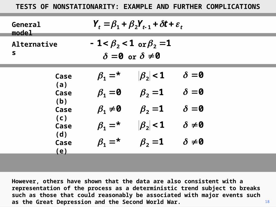
For example, in their influential study, Nelson and Plosser (1982) concluded that the logarithm of GDP, along with several other important macroeconomic variables, was subject to a unit root.


ttt tYY 121

11 2 12 0 0

or

or

12 0

12 01 0

12 01 0

12 0

*1

*1

12 0*1

General model

Alternatives

Case (a)

Case (b)

Case (c)

Case (d)

Case (e)

18

However, others have shown that the data are also consistent with a representation of the process as a deterministic trend subject to breaks such as those that could reasonably be associated with major events such as the Great Depression and the Second World War.


ttt tYY 121

11 2 12 0 0

or

or

12 0

12 01 0

12 01 0

12 0

*1

*1

12 0*1

General model

Alternatives

Case (a)

Case (b)

Case (c)

Case (d)

Case (e)

19

Another layer of complexity is added if the assumption of a constant variance of the disturbance term is relaxed. If this is relaxed, it becomes harder still to discriminate between the competing hypotheses.


ttt tYY 121

11 2 12 0 0

or

or

12 0

12 01 0

12 01 0

12 0

*1

*1

12 0*1

General model

Alternatives

Case (a)

Case (b)

Case (c)

Case (d)

Case (e)

20

In the case of GDP, increased volatility appears to be associated with the same major events that may have been responsible for breaks.


ttt tYY 121

11 2 12 0 0

or

or

12 0

12 01 0

12 01 0

12 0

*1

*1

12 0*1

General model

Alternatives

Case (a)

Case (b)

Case (c)

Case (d)

Case (e)

21

These issues remain an active research area in the literature and make an understanding of the context all the more necessary for the selection of an appropriate representation of a process.


ttt tYY 121

11 2 12 0 0

or

or

12 0

12 01 0

12 01 0

12 0

*1

*1

12 0*1

General model

Alternatives

Case (a)

Case (b)

Case (c)

Case (d)

Case (e)

Copyright Christopher Dougherty 2013.

These slideshows may be downloaded by anyone, anywhere for personal use.

Subject to respect for copyright and, where appropriate, attribution, they may be

used as a resource for teaching an econometrics course. There is no need to

refer to the author.

The content of this slideshow comes from Section 13.4 of C. Dougherty,

Introduction to Econometrics, fourth edition 2011, Oxford University Press.

Additional (free) resources for both students and instructors may be

downloaded from the OUP Online Resource Centre

http://www.oup.com/uk/orc/bin/9780199567089/.

Individuals studying econometrics on their own who feel that they might benefit

from participation in a formal course should consider the London School of

Economics summer school course

EC212 Introduction to Econometrics

http://www2.lse.ac.uk/study/summerSchools/summerSchool/Home.aspx

or the University of London International Programmes distance learning course

20 Elements of Econometrics

www.londoninternational.ac.uk/lse.

2013.08.29

http://www.oup.com/uk/orc/bin/9780199567089/

http://www2.lse.ac.uk/study/summerSchools/summerSchool/Home.aspx

augmented dickey-fuller test equation dependent variable: d(lgdpi) method: least squares sample...

Documents