audio coding - people.cs.nctu.edu.twcmliu/courses/compression/chap14.pdf · overview 2 speech...
TRANSCRIPT

Audio Coding
C.M. LiuPerceptual Signal Processing Lab College of Computer ScienceNational Chiao-Tung University
Office: EC538(03)5731877
http://www.csie.nctu.edu.tw/~cmliu/Courses/Compression/

Overview2
Speech codingBased on a model of speech production
Audio codingBased on a psychoacoustic model of audio perception
General ideaAnalyze the signal and eliminate inaudible sounds
Psychoacoustic model capturesPhysiological perception limits (sensor limitations)Psychological perception limits (signal processing limitations)

Threshold of Audibility3

dB Sound Pressure Level (SPL) Table4

Age-adjusted SPL Table5

Spectral Masking6

Psychoacoustic
IntroductionMasking EffectCritical Band

Psychoacoustic - Introduction
Sound PressureSounds are easily described by mens of the time-varying sound pressure p(t).The unit of sound pressure is the PASCAL (Pa).In psychoacoustics, values of the sound pressure between 10-5 Pa and 102 PA are relevent.
Sound Pressure LevelsNormally used to cope with the broad range of sound pressure.
The reference value of the sound pressure p0 is standardized to p0 = 20 μPa.
L p p dB= 20 0log( / )

Psychoacoustic - Introduction (c.1)
Sound Intensity and Sound Intensity Levels
The reference value I0 is defined as 10 -12 W/m2
Noise DensityWhen dealing with noises, it is advantageous to use density instead of sound intensity
e.g., the sound intensity within a bandwidth of 1 Hz.The noise power density, although not quite correct, is also used.The logarithmic correlate of the density of sound intensity is called sound intensity density level, usually shortened to density level, l. For white nose, l and L are related by the equation
where Δf represents the bandwidth of the sound.
L p p dB I I dB= =20 100 0log( / ) log( / )
L f Hz dB= +[ log( / )]l 10 Δ

Psychoacoustic - Introduction(c.2)
Normative Elements on Human EarThreshold in quiet
A function of frequency that the sound pressure level of a pure tone that is just audibleMasking
Property of the human auditory system by which an audio signal cannot be perceived in the presence of another audio signal.
Masking thresholdA function in frequency and time below which an audio signal cannot be perceived by the human auditory system.
Critical bandLoosely speaking, the perception of a particular frequency, say Ω0, by the auditory system is influenced by energy in a critical band of frequencies around Ω0.The ear acts as a multichannel real-time analyzer with varying sensitivity and bandwidth throughout the audio range.
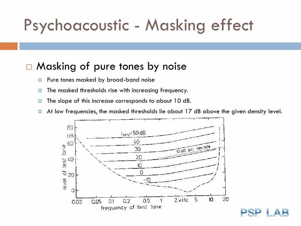
Psychoacoustic - Masking effect
Masking of pure tones by noisePure tones masked by broad-band noise
The masked thresholds rise with increasing frequency.
The slope of this increase corresponds to about 10 dB.
At low frequencies, the masked thresholds lie about 17 dB above the given density level.
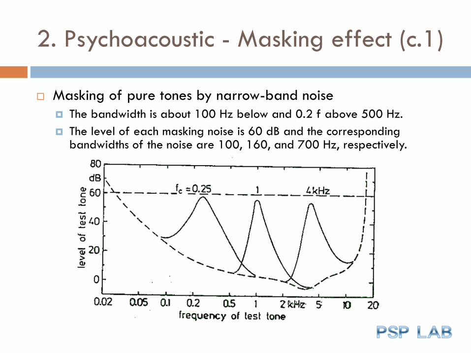
2. Psychoacoustic - Masking effect (c.1)
Masking of pure tones by narrow-band noiseThe bandwidth is about 100 Hz below and 0.2 f above 500 Hz.The level of each masking noise is 60 dB and the corresponding bandwidths of the noise are 100, 160, and 700 Hz, respectively.
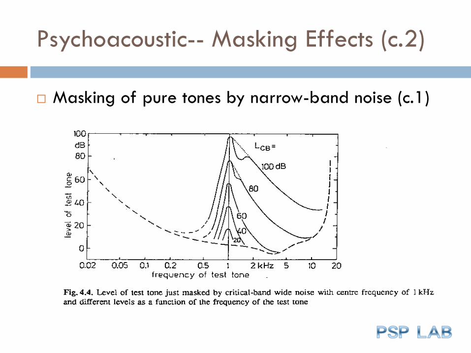
Psychoacoustic-- Masking Effects (c.2)
Masking of pure tones by narrow-band noise (c.1)
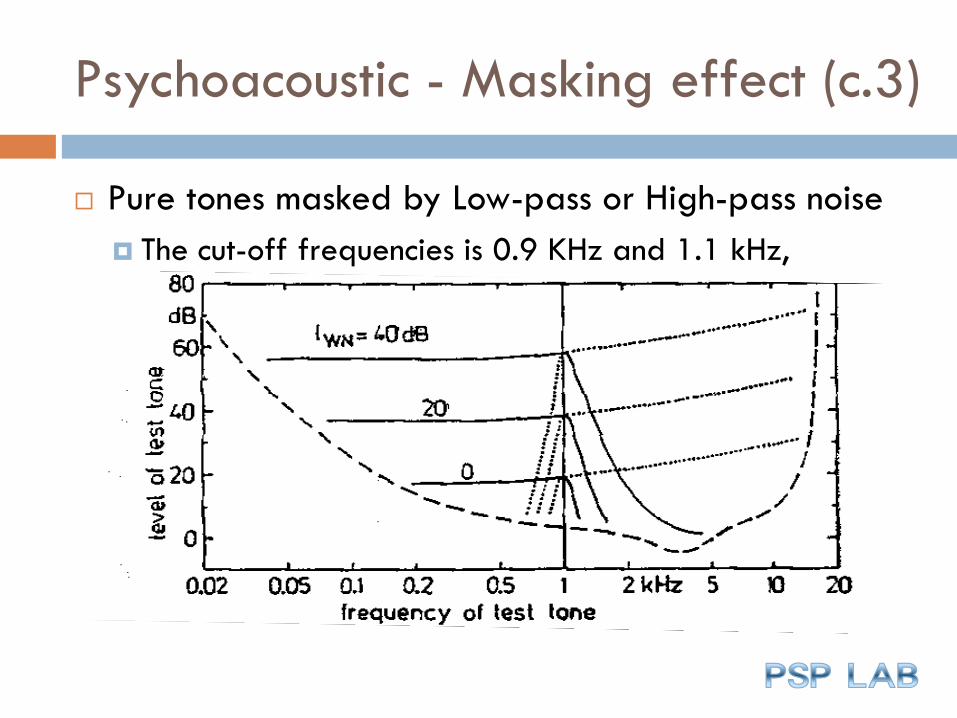
Psychoacoustic - Masking effect (c.3)
Pure tones masked by Low-pass or High-pass noiseThe cut-off frequencies is 0.9 KHz and 1.1 kHz, respectively.

Psychoacoustic - Masking effect (c.4)
Masking of pure tones by pure tonesMasking tone-- 1 kHz, 80 dB.

Psychoacoustic - Masking effect (c.5)
Pure tones masked by pure tones

Psychoacoustic - Masking effect (c.6)
Pure tones masked by complex tones

Psychoacoustic - Masking effect (c.7)
Temporal effectSimultaneous masking
When two signal presence simultaneously , the phenomenon of the weaker signal become inaudible are called simultaneous masking
PremaskingThe test sound has to be a short burst or sound impulse which can be presented before the masker stimulus is switched on
PostmaskingThe test sound is presented after the masker is switched off , then quite pronounced effects occur

Psychoacoustic - Masking effect (c.8)
Premasking & Postmasking do not offer much efforts than simultaneous masking

Temporal Masking20

MPEG Audio Coding21
Video codingMPEG-1 VCD (~VHS)MPEG-2 DVD
Audio coding in MPEGLayers: I, II, III common to both standards111111Commonly: layer III == mp3
Standards:Normative (mandatory) sections
Required for compliance, generally output formatInformative (optional) sections
Not mandatory—e.g., encoding algorithms

MPEG Audio Coding (2)22
LayersBackward compatible
Upwardly more sophisticated
Block-diagram viewInput: 16-bit PCM audio; output: fixed bitrate encoded audio
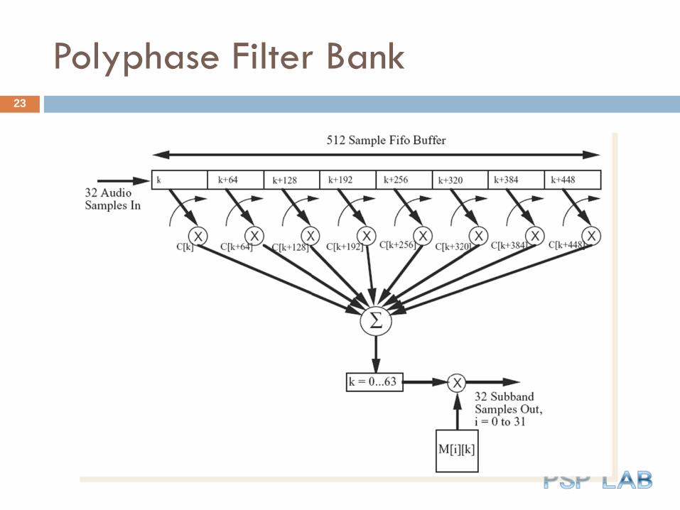
Polyphase Filter Bank23
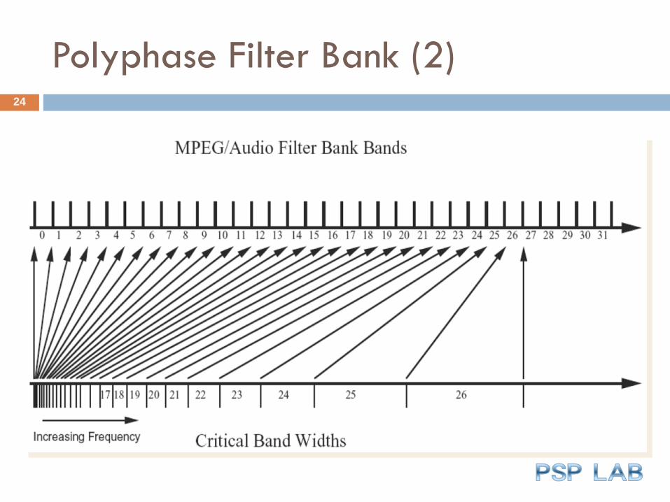
Polyphase Filter Bank (2)24

Polyphase Filter Bank (3)25
Example frequency response:

Psychoacoustic Model26
Model 1:Less computationally expensiveMakes some serious compromises in what it assumes a listener cannot hear
Model 2:Provides more features suited for Layer III coding Assumes more CPU capacity
Psychoacoustic Model (2)27
Time-to-frequency domain conversionPolyphase filter bank + DFT
Model 1:512 samples for Layer I1024 samples for Layers II
Model 2:1024 samples and two calculations per frame (MDCT)

Psychoacoustic Model (3)28
Need to separate sound into “tones” and “noise” componentsModel 1:
Local peaks are tones Remaining spectrum per critical band lumped into noise at a representative frequency.
Model 2:Calculates “tonality” index to determine likelihood of each spectral point being a tone based on previous two analysis windows

Psychoacoustic Model (4)29
“Smear” each signal within its critical bandModel 1: masking functionModel 2: spreading function
Adjust calculated threshold by using a “quiet” mask:A masking threshold for each frequency when no other frequencies are present.
Calculate signal-to-mask (SMR) per bandPass results on to coding/framing unit

Psychoacoustic Model ExampleInput
30

Psychoacoustic Model Example:Transformation to Perceptual Domain
31

Psychoacoustic Model Example:Masking Thresholds
32
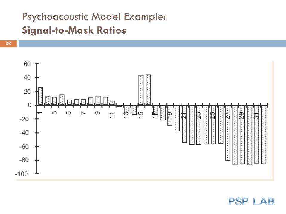
Psychoacoustic Model Example:Signal-to-Mask Ratios
33

Psychoacoustic Model Example:Model Output
34

Layer I Coding: Overview35
Compression—4:1Time frequency mapping
32 subband filtersfilter output down-sampled @ 1/32
Grouping (framing)12 samples x 32 subbands = 384 samples/frame
Each group coded w/ 0-15 bits/sample
Scale factorsUsed to optimize quantizer performanceDetermined based on the 12 samples in the frame63 scale factors 6 bits

Layer-Specific Framing36

Layer I Coding: Bit Allocation37
Task:Determine number of bits to allot for each subband given SMR from psychoacoustic model.
AlgorithmCalculate mask-to-noise ratio:MNR = SNR – SMR (in dB)SNR given by MPEG-I standard (as function of quantization levels)Repeat until no bits to allocate left:
Allocate bit to subband with lowest MNR.Re-calculate MNR for subband w/ allocated bits.

Layer I Coding: Framing38

Layer I Coding: Modes39
StereoTwo independently coded channels, synchronized
Joint stereoTwo channels coded together
‘Mid’ channel: M = (L + R)/2‘Side’ channel: S = (L – R)/2
Dual channelTwo independent channel, unsynchronized
Single channel (mono)One channel

Layer II Coding: Overview40
Generally, Layer I methodology w/ some improvementsCompression—up to 8:1Framing
3 x 12 samples x 32 bands = 1152 samples/frame
Less overhead per frame
Scale factorLayer I: 1 per 12 samples
Layer II: 1 per 24/36 samples

Layer II Coding: Quantization41
Layer I:1 of 14 possible quantizers per band
Layer IIQuantization depends on sampling & bit rates
Some band may get 0 bits“Granules” optimization
Granule = 3 samplesQuantization level based on granules not individual samplesE.g.
3 samples @ 5 q.levels = 35 = 243 possible values 8 bitsAlternative
1 sample @ 5 q.levels = 3 bits x 3 samples 9 bits

Layer II Coding: Framing42

Layer III Coding (mp3)43
ProblemFor low frequencies, Layer I/II bands are significantly wider than critical bands
Obvious solutionIncrease speactral resolution (more bands)
The catchMaintain backward compatibility
SolutionFirst, use the 32-band decompositionThen, use MDCT w/ 50% overlap to subdivide into 6/18

Layer III Coding (2)44
Note that increased spectral resolution lower temporal resolutionQE is spread over entire block
Larger block more error spreading
Normally, backward temporal masking is short (~20ms)QE would appear as a pre-echo
Example:

Layer III Coding (3):MDCT Coefficients
45

Layer III Coding (4):Reconstructed Signal
46

Layer III Coding (5)47
ObservationFor sharp, short sounds, we need small blocks to control the spread of QE
mp3 controls the size of the windowLong window: 36 samplesShort window: 12 samplesStart/stop window: 30 samplesExample

Layer III Coding (6)Window Transition Diagram
48

Layer III Coding (7)49
Long windows32 x 18 = 576 frequencies
Short windows32 x 6 = 192 frequencies
Mixed modeTwo lowest subbands w/ long windows, the rest—short
NoteNumber of samples/frame is always 1152

Layer III Coding (8):Coding & Quantization
50
Outer loop—distortion control loopScale factors assigned in bands of coefficients21 factors for long blocks & 12 for short ones
Inner loop—rate control loopScaled MDCT coeff are quantized
Quantization is nonuniform & compandedHigh-frequency coeff are usually zeroes
Grouped into one region and RL is Huffman codedPreceding coeff of the -1, 0, 1 variety are grouped in quadruplets & Huffman codedRemaining coeff are split into 2-3 groups and appropriately Huffman coded

Layer III Coding (9):Coding & Quantization /2/
51
Control loop:Runs until target rate is achievedModifies quantization/Huffman codes
Distortion loop:Checks psychoacoustic model for allowable distortionModifies scale factors
Bit reservoirCoder runs under target rateMain data may precede frame headerHowever, it cannot split into a following frame

Layer III Coding (10):Coding & Quantization /3/
52

MPEG Audio Data Format53

MPEG Audio Frame Header Format Example
54

A. MPEG1 Audio Coding
FeaturesGeneric ConceptsFeatures of Each Layers Coded Bit-Stream Layer I, II CODECLayer III CODECPsychoacoustic Model 1Psychoacoustic Model 2Stereo ControlConcluding Remarks

A. MPEG1-- Features
Sampling Rate32, 44.1, 48 kHz
Input Resolution16 bits uniform PCM
ModesStereo, Joint Stereo, Dual Channel, and Single
LayersLayer 1: 32 - 448 kbps/channelLayer 2: 32 - 384 kbps/channelLayer 3: 32 - 320 kbps/channel

A. MPEG1-- Generic Concepts
Layer 1: 32 - 448 kbps/channelSimplified of MUSICAMConsumer applications where very low data rates are not mandatory.
Digital home recoding on taps, Winchester discs, or digital optical disks
Layer 2: 32 - 384 kbps/channelNearly identical to MUSICAM except the frame headerConsumer & professional audio
audio broadcasting, television, recording, telecommunication, and multimedia
Layer 3: 32 - 320 kbps/channelMost effective modules in MUSICAM and ASPECMost telecommunication, narrowband ISDN, Professional audio with high weights on very low bit rate.

A. MPEG1-- Features of Each Layers
L a y e r I L a y e r II L a yer IIIA n a ly s is /S y n th es is 32 su bbands 32 su bbands H yb rid (subband +
M D C T )B it a llo c a tio n rep re s e n ta tio n exp lic it index ing Index ingS u g g e s ted p s y c h a c o u s ticm o d e l
M od e l 1 M o d e l 1 M o d e l 2
O u tp u t b it-ra te 32 - 448 K bps 32 - 384 K b ps 32 - 320 K b psE ffic ien t b it-ra te 1 6 0 - 2 2 4 K b p s 9 6 - 1 2 8 K b p s 6 4 - 9 6 K bp sS a m p lin g freq u en cy 32 , 44 .1 , 48 K hz 32 , 44 .1 , 48 K H z 32 , 44 .1 , 48 K H zIn ten s ity s te reo Y es Y es Y e sQ u an tiza tio n U n ifo rm U n ifo rm non -un ifo rmS e g m en ta tio n F ixed F iexe d dynam icE n tro p y co d in g N o N o Y e sS lo t S ize 4 by tes 1 by tes 1 by tesF ra m e S ize 384 sam p les 1152 sam p les 1152 sam p lesF ra m e -s e lf d e c o d ab ility Y es Y es needs p rev ious
fra m esT ec h n ica l o rig in a lity s im p lified
M U S IC A MR e fined M U S IC A M H yb rid from M U S IC A
and A S P E C

A. MPEG1-- Audio Coded BitstreamSyntax
Frame Frame Frame
Header(32)
Error-Check(16) Audio-Data Ancillary
Data
Syn. Word(12) ID
(1)
Layer
(2)
Protection Bit(1)
Bit -RateIndex(4)
Sampling Freq.(2)
Paddingbit(12)
Private-bit(1)
Mode
(2)
Copy right(1)
Emphasis (2)
Mode-Extension (2)

A. MPEG1-- Audio Coded BitstreamSyntax (c.1)
Frame in Layer 1 & 2Part of the bitstream that is decodable by itselfIn Layer 1 it contains information for 384 samples and Layer 2 for 1152 samplesStarts with a syncword and ends just before the next syncword.Consists of an integer number of slots (four bytes in Layer 1 and one in Layer 2).
Frame in Layer 3Part of the bit stream that is decodable with the use of previously acquired side and main information.Contains information for 1152 samplesThe distance between the start of consecutive syncwords is an integer number of slots (one bytes in Layer 3).The audio information belonging to one frame is generally contained between two successive syncwords.

A.MPEG1-- Audio Coded BitstreamSyntax (c.1)
Audio Data for Layer 1 Single Channel
Audio-Data
Bit-Allocation (4)
Scalefactor(6 )
Samples (?)
Bank 0(12 samples for 384 PCMs)
Bank 1 Bank 31
Scalefactor (i+1) =Scalefactor (i)/1.25992104989487
The number of bits per
samples in the band
Normalization Factor of the
samples in the band

A.MPEG1-- Audio Coded BitstreamSyntax (c.2)
Audio Data for Layer 2 Single ChannelThree successive subband samples are grouped to a granule and coded with one code word for quantization steps-- 3, 5, 9.
Audio-Data
Band 0 Band 31
Bit-Allocation (hi-2; mi-3; li-4)
SCFSI(2 )
Scalefactor(6-18 )
Samples (?)
Band i(36 samples for 1152 PCMs)

A.MPEG1-- Audio Coded BitstreamSyntax (c.2)
Audio Data for Layer 3 Side Information 17 or 32 bytes one or two channel
window type, the Huffman Table numbers, the region table appy, scalefactor describtors, a pointer to the end of the main data.
Main DataThe scalefactor and Huffman data
Headerframe 1
side
info
1
Syn
c
Headerframe 2
Headerframe 2
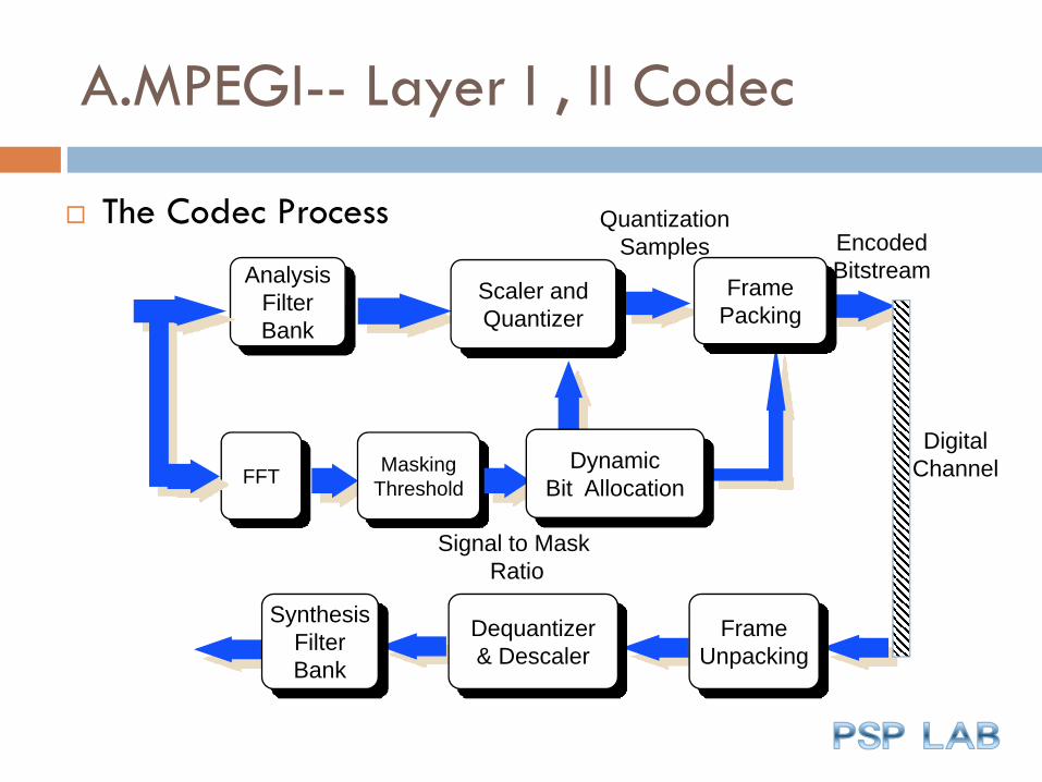
A.MPEGI-- Layer I , II Codec
The Codec Process
Signal to Mask Ratio
QuantizationSamples
Dequantizer & Descaler
EncodedBitstream
SynthesisFilterBank
FrameUnpacking
Frame Packing
AnalysisFilterBank
DigitalChannelFFT Masking
ThresholdDynamic
Bit Allocation
Scaler and Quantizer

A.MPEGI-- Layer I
Bit Rates32, 64, 96, ... 448 kb/s
Sampling Frequency44.1, 48, 32 kHz and one reserved code.
Frame 384 16-bit PCM samples
Encoding MethodThe analysis filter bank and psychoacoustic model execute in parallelFilter Bank
32 equal bandwidth polyphase pseudo-QMF

A.MPEGI-- Layer I (c.1)
ScalefactorA normalization factor before quantization.For each subband, using the max(abs(12 subband samples)) to obtain scalefactor by search table ( Table 3-B.1.)Each scale factor is represented by 6 bits.
Psychoacoustic ModelCalculated in 512 pt. FFT with shift length 384 samples.Provide more sufficient frequency resolution than filter bank.Produces Signal-to-Mask Ratio for each subband.
Dynamic Bit AllocationUse iterative procedure to determine the quantization level for each subband.Let quantization noise is under masking threshold calculated by psychoacoustic model.

A.MPEGI-- Layer I (c.2)
Allocation ProcedureInitially, allocate the quantizer of each subband with zero bit, and we know the SMR of each subbandCalculate available bit number in this frameFrom the quantizer step size find the SNR of each subband( Table 3-C.2)Calculate Mask-to-Noise Ratio (MNR) by MNR = SNR - SMRPick the minimum MNR, allocate one more bit of each sample in this subbandRepeat the above four steps until there is no more bits to allocate

A.MPEGI-- Layer I (c.2)
Quantization and encoding of subband samples (4 bits)From the step size - quantizer table( Table 3C.3), using A, B, and scalefactor to quantize the subband samples:
X1= X / scalefactorX2= A*X1 + BTake the N MSB bitsInvert the MSB bit (avoid confusing with sync. word 1111..1)
PackingMinimum Rate Distortion Curve: Minimum MNR versus number
of bits required to encode a layer 1 frame determined for a
particular frame.
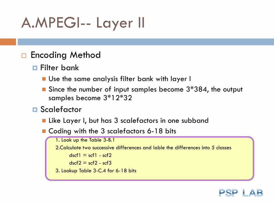
A.MPEGI-- Layer II
Encoding MethodFilter bank
Use the same analysis filter bank with layer ISince the number of input samples become 3*384, the output samples become 3*12*32
ScalefactorLike Layer I, but has 3 scalefactors in one subbandCoding with the 3 scalefactors 6-18 bits
1. Look up the Table 3-B.12.Calculate two successive differences and lable the differences into 5 classes
dscf1 = scf1 - scf2dscf2 = scf2 - scf3
3. Lookup Table 3-C.4 for 6-18 bits

A.MPEGI-- Layer II(c.1)
Psychoacoustic modelUse 1024 pt. FFT with shiftlength 1152 pt.Produce Signal-to-Mask Ratio (SMR), like layer I
Dynamic bit allocationPerforms like layer I
Quantization and encoding of subband samplesLike Layer I, but has finer quantization with up to 16 b amplitude.The number of available quantizers decreases with increased subbabd index.If quantization level is 3, 5, or 9, 3 consecutive samples are coded into one codeword
eg. v3=9z+3y+x (3 based)eg. v5=25z+5y+x (5 based)eg. v9=81z+9y+x (3 based)
Packing

A.MPEGI-- Layer I, II Decoder
Layer I, II DecodingNo Psychacoustic Model is needed.The computation power for Encoder and Decoder for Layer 1 is about 2:1 and Layer 2 is 3:1.
Begin Input Encoded Bit Stream
Decoding of Bit Allocation
Decoding of Scalfactor
Requantization of Samples
End Output PCM Samples
Synthesis Subband Filters

A.MPEGI-- Synthesis Subband Filter Flow Chart
Begin
Input 32 New ubband Samples Si i = 0, ..., 31
For i = 1023 down to 64 do V(i) = V(i-64)
For i =0 to 63 do
V N Si ikk
k==∑
0
31
Build a 512 avlue vector U for i = 0 to 7 do for j=0 to 31 do U(64i+j]=V[128i+j];
U[64i+32+j] = V[128i+96+j]
Window by 512 coefficients Produce vector W for i =0 to
511 do Wi = Ui *Di
Calculate 32 samples for j =0 to 31 do
S Wj j ik
= +=∑ 32
0
15
Ouput 32 reconstructed PCM Samples
End

A.MPEGI-- Layer III Codec
SynthesisFilterBank
HuffmanCoding
MaskingThreshold
Scalerand
Quantizer
AnalysisFilterBank
MDCT withdynamic
windowing
FFTCoding of
SideInformation
Packing
Unpacking
HuffmanCoding
Dequantizer& Descaler
MDCT withdynamic
windowing
Decoding ofSide
Information

A.MPEGI-- Layer III Codec
The coder process:
Layer I Analysis
Filter
inputsample
bufferfor36
subband 0samples
MDCToutputlong:18short: 6
bufferfor36
subband 31samples
MDCT
Aliasing
....
block:long: 36short :3 * 12
Psychoacoustic Model :decide block type and allow distortion
....
block:long: 36short :3 * 12
Scalerand
quan-tizer
Huff-man
coding
codingof
sideinformation
PACKING

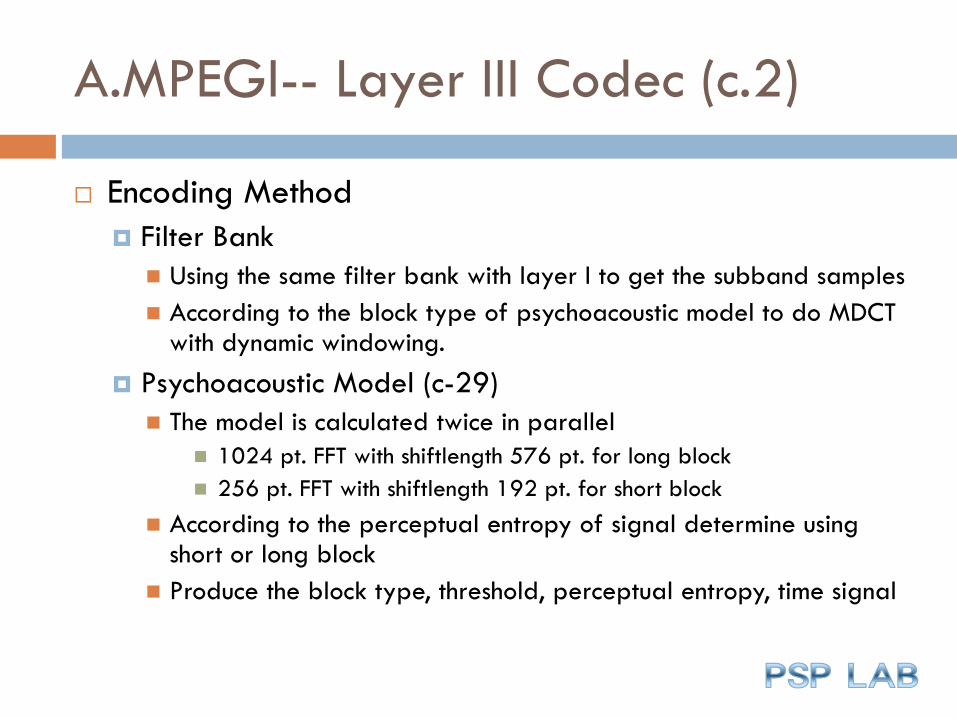
A.MPEGI-- Layer III Codec (c.1)
FeaturesHybrid polyphase/MDCT filter bank.Different frequency resolution for the attributes of samples. Nonuniform quantization and Huffman coding are used to increase coding efficiency.A buffer technique called bit reservoir is used to maintain coding efficiency and to keep the quantization noise below the masking threshold.the scalefactors of gr1, gr2 can be grouped.Long blocks and short blocks are switched for controlling pre-echo effects. Long block : the 576 frequence lines can be divided to 21 scalefactor bandsShort block : the 192 frequence lines can be devided to 12 scalefactor bands
A.MPEGI-- Layer III Codec (c.2)
Encoding MethodFilter Bank
Using the same filter bank with layer I to get the subband samplesAccording to the block type of psychoacoustic model to do MDCT with dynamic windowing.
Psychoacoustic Model (c-29)The model is calculated twice in parallel
1024 pt. FFT with shiftlength 576 pt. for long block256 pt. FFT with shiftlength 192 pt. for short block
According to the perceptual entropy of signal determine using short or long blockProduce the block type, threshold, perceptual entropy, time signal

A.MPEGI-- Layer III Codec (c.3)
QuantizationNonuniform quantization
xr(i): absolute value of frequency line at index iquant: actural quantizer step sizenint: nearest integer functionquantized absolute value at index i.
Bigger values are quantized less accurately than smaller values.Huffman Coding
A series of zero at high frequencies is coded by run-length coding.All the contiguous quadruples consisting of values 0, -1, 1 are assigned to the count1 section (two tables).The remaining pairs whose absolute values form the last section (32 tables).
is i n xr i quant( ) int((( ( ) / ) ) . ).= −0 75 00946

A.MPEGI-- Layer III Codec (c.4)
The choice of Humman table depends largly on the dynamic range of the values.
AllocationUsing two iteration loops to control the distortion be under the masking thresholdInner loop: quantize the input vector and increases the quantizer step size until output vector can be coded with the available amount of bits.Outer loop: Check the output from inner loop, if the allow distortion is exceeded, amplifies the scalefactor band and call the inner loop again (Noise allocation)
Bit Reservoir TechniqueA buffer techniqueThe amount of bits corresponding to a frame is no longer constant, but varies with a constant long term average.

A.MPEGI-- Layer III Codec (c.5)
Window switching logic
normal
shortstop
startattack
attack
attackattack
no attack
no attack
no attack

A.MPEGI-- Layer III Codec (c.6)
Four Types of Window Functions

A.MPEGI-- Layer III Codec (c.7)
Illustration of the window switching decision
normal block startblock
shortblock
stopblock
normalblock
Input Sound Signal
t
t

A.MPEGI-- Layer III Codec (c.8)
Scalefactor Bands576 spectral lines for the long MDCT are grouped into 21 scalefactorbands.192 spectral lines for short MDCT are grouped into 12 scalefactor bands.Scalefactors are sent either for each granule in a frame or for both granules together, depending upon the contents of the scalefactor selection information (sfsi) variable.The 21 scalefactor bands are assigned to four groups.
For each group, a scalefactor selector information (1 bit) for one factor for a granule or for bith granules.
The number of bits of the scalefactor is specified by a four bit variable called scalefac_compress.The 21 bands are devided into two groups 0-10 and 11-20. The scalefac_compress variable indexes a table which returns two numbers called slen1 and slen2, the number of bits assigned to the bands in groups 1 and 2.

A.MPEGI-- Layer III Codec (c.8)
Allocation FunctionOuter loop adjusts the scale factor to shape the noise spectrum.Inner loop sets the global_gain to the value which brings the number of bits to encode the granule to the value closest but not exceeding maxbits.Duriing the initial stage, the maximum allowable quantization noise, xmin is determined for each scale factor band.The maximum number of bits for encoding the granule, maxbits, is determined and all scalfactors are initialized to their lowest values.The iteration terminates when the scalefactors are increased in small increments until the quantization noise is below xmin or until the scalefactors cannot be increased any more.
The main bottleneck to the iteration occurs in the inner loop where the number of bits needed to encode the granule is determined. This involves
quantizing the 576 values and counting the number of bits needed to Huffman encode the quadruples and big_value pair.

A.MPEGI-- Layer III Codec (c.9)
global_gain SNR576 spectral lines
Xmin

A.MPEGI-- Layer III Codec (c.9)
Decoding MethodHuffman decodingRequantization and all scalingSynthesis filter bank [ preprocess alias reduction ]IMDCTOverlapping and add with previous block

A.MPEGI-- Synthesis Subband Filter Flow Chart
Begin
Get Bit Stream, Find Header
Decode Scalefactor
Reorder if (blocksplit_flag) and (block_type ==2)
Alias Cancellation
Synthesize via MDCT & Overlap-Add (Using either 18 or 666 depending on blocksplit_flag and block_type [gr])
Synthesize via Polyphase MDCT
End
Decode Samples
Inverse Quantize Samples
Output Samples

A.MPEGI-- Psychoacoustic Model I
InputLayer I: 384 PCM samples frame; Layer II: 3*384 PCM samples
OutputSignal-to-Mask Ratio (SMR) for each subband
StepsFFT Analysis
Find the corresponding data segment with length N=512 for layer I, and 1024 for layers II and III.
s(l) 0<=l <= N-1Hanning window
h i i N i N( ) / * . *{ cos[ ( ) / ( )]};= − − ≤ ≤ −8 3 05 1 2 1 0 1π

A.MPEGI -- Psychoacoustic Model I(c.1)
Power Density Spectrum
Determination of Sound Pressure LevelDetermine the sound pressure level in each subband, Lsb(n) by choosing one largest energy to represent this subband
X(k) is the sound pressure level of the spectral line with index k of the FFT with the maximum amplitude in the frequency range corresponding to subband n.The -10dB term corrects for the difference between peak and RMS level.
L MAXX k insubband n
X k scf n dBsb = −( )
[ ( ), log( ( ) * ) ]max20 32768 10
X kN
h l s l e dB k Njkl N
l
N
( ) log ( ) ( ) , , , //= =−
=
−
∑10 1 0 1 22
0
1 2π

A.MPEGI -- Psychoacoustic Model I (c.2)
Determine the Threshold in QuietThe threshold in quiet LTq(k) is called absolute threshold.These tables depend on the sampling rate of the input PCM signal (see Table 3-D.1).An offset depending on the overall bit rate is used for the absolute threshold. This offset is -12 dB for bit rates >=96 kbits/s and 0 dB for bit rates <98 kbits/s per channel.
Finding of Tonal and Nontonal ComponentsConcepts: The different masking effect between tonal and non-
tonal soundLabelling of local maximum.
X(k) > X(k-1) and X(k) >= X(k+1)X(k) - X(k+j) >= 7dB; the range of j depends on Layers and frequency.

A.MPEGI -- Psychoacoustic Model I (c.3)
Listing of tonal components and calculation of the sound pressure level.
Index number kSound pressure level Xtm(k) = X(k-1) + X(k) + X(k+1) Tonal Flag.
Listing of non-tonal components and calculation of the power.
The power of the spectral lines are summed to form the sound pressure level of the new non-tonal component corresponding to that critical band.Index number k of the spectral line nearest to the geometric mean of the critical band.(see Table 3-D.2, Layer1: 23 critical bands for 32kHz, 24 bands for 44.1k; 25 for 48k; Layer 2: 25 bands for 32 KHz, 26 bands for 44.1 and 48 kHz)Sound pressure level Xnm(k) in dBNon-tonal flag

A.MPEGI -- Psychoacoustic Model I (c.4)
FFT Spectrum Magnified Portion
Power Spectrum Decimated Spectrum

A.MPEGI -- Psychoacoustic Model I (c.5)
Decimation of the Masking Components.Concepts: Reduce the number of MaskersEliminate the tonal Xtm(k) and non-tonal Xnm(k) components below absolute thresholdEliminate the tonal components within a distance of 0.5 Bark, remove the smaller components from tonal lists
Calculation of the Individual Masking ThresholdsOf the original domain samples indexed by k, only a subset of the samples indexed by i are considered for threshold calculation.Calculate individual tonal and non-tonal masking threshold to predetermined frequencyLTtm[z(j),z(i)] = Xtm[z(j)] + avtm[z(j)]+vf[z(j),z(i)] dBLTnm[z(j),z(i)] = Xnm[z(j)] + avnm[z(j)]+vf[z(j),z(i)] dB
avtm = -1.525 - 0.275*z(j) - 4.5 dBavnm = - 1.525 - 0.175*z(j) - 0.5 dB

A.MPEGI -- Psychoacoustic Model I (c.6)
Non-Tonal Components Decimated Non-Tonal Components
NonTonal Masking
Tonal Masking

A.MPEGI -- Psychoacoustic Model I (c.7)
vf = 17(dz +1) - (0.4*X(z(j)]+6) dB for -3 <= dz < 0.1 Barkvf = (0.4*X[z(j)] + 6)*dz dB for -1 <= dz < 0 Barkvf = -17 dB for 0 <=dz < 0 Barkvf = -(dz-1)*(17-0.15X[z(j)]) - 17 dB for 1 <= dz < 8 Bark
Determine the Global Masking ThresholdCalculate total masking energy for every frequency component (normal square amplitude scale).
The summation can be reduced to +8 to -3 Barks
LT igLT i LT j i LT j i
j
n
j
mq tm nm( ) log( ( ) / ( , ) / ( , ) / )= + +
==∑∑10 10 10 1010 10 10
11
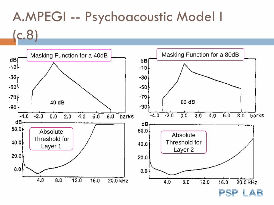
A.MPEGI -- Psychoacoustic Model I (c.8)
Masking Function for a 40dB Masking Function for a 80dB
Absolute Threshold for
Layer 1
Absolute Threshold for
Layer 2

A.MPEGI-- Psychoacoustic Model I (c.8)
Determine the Minimum Masking Threshold
Determine the minimum masking level in each subband.
Calculate the signal-to-mask ratioSMRsb (n) = Lsb(n) - LTmin(n) dB
LT n MINf i insubbandn
LT i dBgmin ( )( )
[ ( )]=
Global masking threshold
Minimum masking threshold
Final signal-to-mask ratio

A.MPEGI -- Psychoacoustic Model II
InputShort block: 192 new sample with 256 pt. FFTLong block: 576 new sample with 1024 pt. FFT
OutputBlock type (Layer III)Signal-to-Mask Ratio (SMR) for each scalefactor band
Calculation of block type and SMRFFT: Using Hanning window, get the polar representation of the transform rw and fw
Use a polynomial predictor to predict magnitude and phase( ) ( )( ) ( )
Ã.
Ã.
r r t r t
f f t f t
w w w
w w w
= − − −
= − − −
2 0 1 2
2 0 1 2

A.MPEGI -- Psychoacoustic Model II (c.1)
Calculate Euclidian distance between predict value cw for each line.
Calculate energy & unpredictability in each partition.(Table 3-D.3)A resolution of approximately one FFT line or 1/3 critical band.The Table Contents
Index of the partition, bLowest frequency line, wlowb.Highest frequency line, whighbThe median Bark value, bvalbA lower limit for the SNR in the partition that controls
stereo unmasking effects, minvalbThe value for tonal masking noise for that partition, TMNb
( ) ( )( )c
r f r f r f r f
r abs rw
w w w w w w w w
w w
=− + −⎛
⎝⎜⎞⎠⎟
+
cosÃcos
Ãsin
Ãsin
Ã
Ã
.2 2
0 5
e r
c r c
b ww w l o w b
w h i g h b
b w ww w l o w b
w h i g h b
=
=
=
=
∑
∑
2
2
;
Unpredictivity Measure

A.MPEGI -- Psychoacoustic Model II (c.2)
Partition number-critical band rate
Conversion from spectral
line to partition number
Fourier Power Spectrum
Unpredictability
Partition energy & Partitioned
Unpredictability
Convolved partitioned energy &
unpredictability

A.MPEGI -- Psychoacoustic Model II (c.3)
Calculate energy(ecbb) & noise(cbb) masking effects and normalize them(cbb,enb)
Convert chaos measure cbb to tonality tbb0.05< cbb< 0.5 => 0< tbb< 1tbb= -0.299-0.43 loge(cbb)
( )
( )
ecb e sprdngf bval bval
ct c sprdngf bval bval
b bb bb bbb
b
b bb bb bbb
b
=
=
=
=
∑
∑
,
,
max
max1
1( )∑
=
=
=
=
max
0,
1*
b
bbbbb
b
bbb
b
bb
bvalbvalsprdngfrnorm
rnormecbenecbctcb
enb
tbb

A.MPEGI -- Psychoacoustic Model II (c.4)
According to the tonality(tbb) to calculate spread threshold(SNRb) (TMN, NMT)
SNRb= max(minvalb, tbb*TMNb+ (1-tbb)* 5.5)Calculate the power ratio of SNRb
Renormalization ( nbw)
Include the absolute threshold for final Energy Threshold of audibility
b cn b e n b c
b
S N R
b b b
b
==
−
1 0 1 0
*
nb nbwhight w w loww
b
b b
=− − + 1
thr nb absthrw w w= m ax( , )
SNRb

A.MPEGI-- Psychoacoustic Model II (c.5)
Pre-Echo Control (C-30)
thr(b)= max(qthr(b), nbb(b), nbb_I(b), nbb_II(b))
nbb_I(b) = 2*nbb(b) from the last block
nbb_II(b) = 16*nbb(b) from the block before the last block
Calculate SMR in each scalefactor band
epart rn wwlown
whighn
= ∑ 2
npart thrw for narrow scalfactor band
npart thrwlow thrwhigh whigh wlowfor wide scalefactor band
nwlown
whighn
n n n h n
=
= − +
∑min( , . . . , ) * ( )1
SM R epartnpartn
n
n
= 10 10log ( )

A.MPEGI -- Psychoacoustic Model II (c.6)
Masking Threshold
Masking Threshold mapped to Fourier spectral domain
Signal-to-masker ratio
Spreading Function Tone Masking Function The minval function

A.MPEGI-- Adaptation of the Psychoacoustic Model 2 for Layer 3
Tone masking ratio is now fixed at 29dB and the noise masking tone is 6 dB.Mainval function is specified as a function of partition number.A perceptual entropy is returned.
calculated from the weighted average of the logarithm of the ratio of the masking threshold over the energy for all partitions.The ratio is then transformed to the scale factor bands.
The unpredictability measure is now computed using long FFTs (1024)for the first 6 lines and short FFTs(256) for the next 200 lines, for the remaining lines, the unpredictivity assumes a value of 0.4.

A.MPEGI-- Adaptation of the Psychoacoustic Model 2 for Layer 3
Preecho control is incorporated by computing a new threshold based on the current threshold and the thresholds calculated for the previous two blocks.
Spreading Function
Minval Function

A.MPEGI-- Intensity Stereo
ConceptsAt high frequency, the location of the stereophonuc image within a critical band is determined by the temporal envelope and not by the temporal fine structure.
Technique (adopted in Layer 1&2)For some subbands, instead of transmitting separate left and right subband samples only the sum-signal is transmitted, but with the scalefactors for both the left and right channels.The quantization, coding, bit allocation are preferred in the same way as in independent coding.

A.MPEGI-- Intensity Stereo and MS Stereo
MS_Stereo SwitchingSwitch is on when
The values rli and rri correspond to the energies of the FFT line spectrum of the left and right channel calculated within the psychoacoustic model.
MS_Matrix
[ ] . [ ]rl rr rl rrii
i ii
i2
0
5112 2
0
51120 8
= =∑ ∑+ < +
M R L S R Li
i ii
i i=+
=−
2 2;

A.MPEGI-- Concluding Remarks
Features Layer I Layer II Layer III
Mapping into subband filtering subband + overlapfrequency into 32 equally transform with coefficients spaced bands dynamic windowing.
Scaling one scalefactor for 1 to 3 for by clustering of factor 12 consecutive 36 frequency into
output consecutive bands, 1 per bandeach band output
each band
Bit allocation found by iteration based on MNR based on SMR(bit allocation ) (noise allocation )

B. MPEG II & IV
MPEG IIThe syntax, semantics, coding techniques are maintained.Multichannel and multilingual audio.Lower sampling frequencies (16, 22.05, 24 kHz) and lower bit rates.Multichannel Featues: 3/2, 3/1, 3/0, 2/2, 2/1. 2/0, 1/0) Downward compatibilityNBC (Non backward compatible ) syntax will be defined.
MPEG IVAddress at low and very low bit rates
a stereo audio signal over a 64 kb/s rate channelIn the field of digital multichannel surround systems
The use of interchannel correlations and interchannel masking effects

Remark A: Derivation of the Analysis/Synthesis Filters for MPEGI-- Audio
The Modulated Filter BanksThe Analysis Filters hk(n)
where L and M are the filter length and filterbank number.
The Synthesis Filters fk(n)
h n p n k nL
Mk k( ) ( )cos ( )( )= + −
−−⎡
⎣⎢
⎤
⎦⎥
1
2
1
2
π φ
f n p n k nL
Mk k( ) ( )cos ( )( )= + −
−+⎡
⎣⎢
⎤
⎦⎥
1
2
1
2
π φ

A.1 Requirements for PR
The phase restriction
where p is a constant.
The selection for the h(n)
h n h L n h m iM h m i M si
LM
s
( ) ( ); ( ) ( ( ) ) ( )= − − + + + ==
− −
∑1 20
2 1
δ
φ φ πk k p− = +−1 2 1
2( )

A.2 The parameters in MPEG 1-- Layer 1&2
L=513, p=512/2M=8The phase
The Analysis & Synthesis Filters
φ π πk k p k= + + = + +( )( ) ( )( )1
22 1
212
16 12
h n p n k nM
Mk ( ) ( )cos ( )( )= + −⎡
⎣⎢
⎤
⎦⎥
1
2 2
1
f n p n k nM
Mk ( ) ( )cos ( )( )= + +⎡
⎣⎢
⎤
⎦⎥
1
2 2
1

A.3 Derivation of the Analysis Filter Banks
The Analysis FiltersX m h n x n h r x mM r
x mM r p r k r
Let z r x mM r p r
So
X m z r k r
Let r
k k n mM k
r
L
r
L
k
r
L
( ) ( )* ( ) ( ) ( )
( ) ( ) cos ( )( )
( ) ( ) ( )
( ) ( ) cos ( )( )
= = −
= − + −⎡
⎣⎢
⎤
⎦⎥
= −
= + −⎡
⎣⎢
⎤
⎦⎥
=
==
−
=
−
=
−
∑
∑
∑
0
1
0
1
0
1
1
216
32
1
216
32
π
π
64 0 1 7 0 1 63
64 11
216
320
7
0
63
l s where l s
So X m z l s k skl
ls
+ = =
= + − + −⎡
⎣⎢⎤
⎦⎥==∑∑
, , ,..., ; , , ...,
( ) ( )( ) cos ( )( )π

A.4 The Synthesis Filters
y n y n X r f n r X r p n r k n r
L et n l s s b lock num ber l
y l s p l r s
k
k
k
rk
k
rk
( ) ( ) ( ) ( ) ( ) ( ) cos ( )( )
; , , ..., ; , , ...........
( ) ( ( )
= = − = − + − +⎡
⎣⎢⎤
⎦⎥
= + = =
+ = − +
= = −∞
∞
= ==∑ ∑∑ ∑∑
0
31
0
31
0
15
0
31
32 321
232 16
32
32 0 1 31 0 1
32 32
π
) ( ) cos ( )( ( ) )
( ) ( ) ( ) cos ( )( ) ( ) ( ; )
( ;
r
k
k
q
k
k q
X r k l r s
L et q l r
y l s p q s X l q k q s p q s U l q s
w here U l
= −∞
∞
=
= = =
∑ ∑
∑ ∑ ∑
+ − + +⎡
⎣⎢⎤
⎦⎥
= −
+ = + − + + +⎡
⎣⎢⎤
⎦⎥= + +
0
31
0
15
0
31
0
15
1
232 16
32
32 321
232 16
3232 32
π
π
321
232 16
32
641
216
320 1 63
2
32 64
0
31
0
31
q s X l q k q s
D efineV l j i X l i k j w here j
So if q even i
U l q s U l i s X l q
k
k
k
k
k
+ = − + + +⎡
⎣⎢
⎤
⎦⎥
+ = − + +⎡
⎣⎢
⎤
⎦⎥ =
= =
+ = + = −
=
=
∑
∑
) ( ) cos ( )( )
( ; ) ( ) cos ( )( ) , , ....,
;
( ; ) ( ; ) ( ) cos
π
π
k
ik
k
i
k
k
k i s
X l i k s V l i s
If q odd i
U l q s U l i s X l q k
=
=
=
∑
∑
∑
+ + +⎡
⎣⎢
⎤
⎦⎥
= − − + +⎡
⎣⎢⎤
⎦⎥= − +
= = +
+ = + + = − +
0
31
0
31
0
31
1
264 16
32
1 21
216
321 128
2 1
32 64 321
2
( )( )
( ) ( ) cos ( )( ) ( ) ( , )
;
( ; ) ( ; ) ( ) cos ( )(
π
π
s
V l i si
+ +⎡
⎣⎢
⎤
⎦⎥
= − + +
32 1632
1 128 96
)
( ) ( , )
π

Remark B Windows
Short-Time Spectral Analysis
Role of WindowsThe window, w(n), determines the portion of the signals that is to be processed by zeroing out the signal outside the region of interest.The ideal window frequency response has a very narrow main lobe which increases the resoluion, and no side lobes (or frequency leakage).
S e w k n s n ekj j n
n
( ) ( ) ( )ω ω= − −
=−∞
∞
∑

B.1 Windowing Functions--
SomeExamples

B.2 Windowing Functions-- Time Shape

B.3 Windowing Functions--Performance

B.4 Windowing Functions-- Low-Pass FIR Filter Design with Windowing
Rectangular Window(M=61) Hamming Window (M=61)
Blackman Window (M=61) Kaiser Window (M=61)

Remark C: QMF/DCT/MDCT
QMF
h n h n for n and n Nh n h N n n Nh n h N n n Nh n h n
H e H e
l u
l l
u u
un
l
lj
uj
( ) ( )( ) ( ) , , , /( ) ( ) , , ... /( ) ( ) ( )
( ) ( )
= = < ≥= − − = −= − − − = −
= −
+ =
0 01 0 1 2 2 1
1 0 1 2 11
12 2ω ω

C.2 DCT
DCT
IDCT2D DCT & 2D IDCT
F uN
u x n n uN
u N
u for u
un
N
( ) ( ) ( ) cos ( ) , , ... ,
( ) / ; ( )
=+
= −
= = ≠=
−
∑2 2 12
0 1 1
0 1 2 1 00
1
α π
α α
x nN
u F u n uN
n Nn
N
( ) ( ) ( ) cos ( ) , , ... ,=+
= −=
−
∑2 2 12
0 1 10
1
α π
F u vN
u v x n n uN
m uN
u v if u vm
N
n
N
( , ) ( ) ( )[ ( ) cos ( ) cos ( )
( ) ( ) / ; ( ) ( ) ,
=+ +
= = = = ≠ ≠=
−
=
−
∑∑2 2 12
2 12
0 0 1 2 1 0 00
1
0
1
α α π π
α α α α
x m nN
u v F u v m uN
n uNv
N
u
N
( , ) ( ) ( ) ( , ) cos ( ) cos ( )=
+ +
=
−
=
−
∑∑2 2 12
2 120
1
0
1
α α π π

C.3 MDCT
MDCT
F u h n x nN
u n N u
h N n h nh N n h N n for n N
h n nN
n
N
( ) ( ) ( ) cos ( )( ) , ,
( ) ( )( ) ( ) .
( ) sin ( )
= + + +⎡⎣⎢
⎤⎦⎥
=
− − = =
+ + − − = ≤ <
= ± +⎡⎣⎢
⎤⎦⎥
=
−
∑ 12
2 1 2 1 0 1
1 22 1 2 0
2 12 2
0
2 1
2 2
2 2 2
π