audio coding based on integer transforms - willkommen ... · audio coding based on integer...
TRANSCRIPT

Audio Coding Based on Integer Transforms
Dissertation zur Erlangung des akademischen Grades
Doktor-Ingenieur (Dr.-Ing.)
vorgelegt der Fakultat fur Elektrotechnik und Informationstechnik
der Technischen Universitat Ilmenau
von Dipl.-Math. Ralf Geiger
Gutachter:
Univ.-Prof. Dr.-Ing. Karlheinz Brandenburg
Univ.-Prof. Dr.-Ing. Walter Kellermann
Dr.-Ing. Jurgen Herre
Tag der Einreichung: 11. Oktober 2004
Tag der Verteidigung: 2. November 2007
urn:nbn:de:gbv:ilm1-2007000278

Abstract
In recent years audio coding has become a very popular field for research and applica-
tions. Especially perceptual audio coding schemes, such as MPEG-1 Layer-3 (MP3)
and MPEG-2 Advanced Audio Coding (AAC), are widely used for efficient storage
and transmission of music signals. Nevertheless, for professional applications, such
as archiving and transmission in studio environments, lossless audio coding schemes
are considered more appropriate.
Traditionally, the technical approaches used in perceptual and lossless audio cod-
ing have been separate worlds. In perceptual audio coding, the use of filter banks,
such as the lapped orthogonal transform “Modified Discrete Cosine Transform”
(MDCT), has been the approach of choice being used by many state of the art
coding schemes. On the other hand, lossless audio coding schemes mostly employ
predictive coding of waveforms to remove redundancy. Only few attempts have been
made so far to use transform coding for the purpose of lossless audio coding.
This work presents a new approach of applying the lifting scheme to lapped trans-
forms used in perceptual audio coding. This allows for an invertible integer-to-
integer approximation of the original transform, e.g. the IntMDCT as an integer
approximation of the MDCT. The same technique can also be applied to low-delay
filter banks. A generalized, multi-dimensional lifting approach and a noise-shaping
technique are introduced, allowing to further optimize the accuracy of the approxi-
mation to the original transform.
Based on these new integer transforms, this work presents new audio coding
schemes and applications. The audio coding applications cover lossless audio cod-
ing, scalable lossless enhancement of a perceptual audio coder and fine-grain scalable
perceptual and lossless audio coding. Finally an approach to data hiding with high
data rates in uncompressed audio signals based on integer transforms is described.
2

Zusammenfassung
Die Audiocodierung hat sich in den letzten Jahren zu einem sehr popularen For-
schungs- und Anwendungsgebiet entwickelt. Insbesondere gehorangepaßte Verfahren
zur Audiocodierung, wie etwa MPEG-1 Layer-3 (MP3) oder MPEG-2 Advanced
Audio Coding (AAC), werden haufig zur effizienten Speicherung und Ubertragung
von Audiosignalen verwendet. Fur professionelle Anwendungen, wie etwa die Ar-
chivierung und Ubertragung im Studiobereich, ist hingegen eher eine verlustlose
Audiocodierung angebracht.
Die bisherigen Ansatze fur gehorangepaßte und verlustlose Audiocodierung sind
technisch vollig verschieden. Moderne gehorangepaßte Audiocoder basieren meist
auf Filterbanken, wie etwa der uberlappenden orthogonalen Transformation “Mod-
ifizierte Diskrete Cosinus-Transformation” (MDCT). Verlustlose Audiocoder hinge-
gen verwenden meist pradiktive Codierung zur Redundanzreduktion. Nur wenige
Ansatze zur transformationsbasierten verlustlosen Audiocodierung wurden bisher
versucht.
Diese Arbeit prasentiert einen neuen Ansatz hierzu, der das Lifting-Schema auf
die in der gehorangepaßten Audiocodierung verwendeten uberlappenden Transfor-
mationen anwendet. Dies ermoglicht eine invertierbare Integer-Approximation der
ursprunglichen Transformation, z.B. die IntMDCT als Integer-Approximation der
MDCT. Die selbe Technik kann auch fur Filterbanke mit niedriger Systemver-
zogerung angewandt werden. Weiterhin ermoglichen ein neuer, mehrdimensionaler
Lifting-Ansatz und eine Technik zur Spektralformung von Quantisierungsfehlern
eine Verbesserung der Approximation der ursprunglichen Transformation.
Basierend auf diesen neuen Integer-Transformationen werden in dieser Arbeit
neue Verfahren zur Audiocodierung vorgestellt. Die Verfahren umfassen verlust-
lose Audiocodierung, eine skalierbare verlustlose Erweiterung eines gehorangepaßten
Audiocoders und einen integrierten Ansatz zur fein skalierbaren gehorangepaßten
und verlustlosen Audiocodierung. Schließlich wird mit Hilfe der Integer-Transfor-
mationen ein neuer Ansatz zur unhorbaren Einbettung von Daten mit hohen Daten-
raten in unkomprimierte Audiosignale vorgestellt.
3

Contents
1 Introduction 7
2 Overview 9
3 State of the Art 10
3.1 Filter Banks and Transforms . . . . . . . . . . . . . . . . . . . . . . . 10
3.1.1 General Structure of Filter Banks . . . . . . . . . . . . . . . . 10
3.1.2 Polyphase Decomposition . . . . . . . . . . . . . . . . . . . . 12
3.1.3 Block Transforms . . . . . . . . . . . . . . . . . . . . . . . . . 15
3.1.4 The MDCT . . . . . . . . . . . . . . . . . . . . . . . . . . . . 18
3.1.5 MDCT by Windowing / Time Domain Aliasing and DCTIV . 21
3.1.6 Low Delay Filter Banks . . . . . . . . . . . . . . . . . . . . . 23
3.2 Data Compression by Entropy Coding . . . . . . . . . . . . . . . . . 27
3.2.1 Huffman Coding . . . . . . . . . . . . . . . . . . . . . . . . . 27
3.2.2 Arithmetic Coding . . . . . . . . . . . . . . . . . . . . . . . . 27
3.3 Perceptual Audio Coding . . . . . . . . . . . . . . . . . . . . . . . . . 28
3.3.1 Basic Principles . . . . . . . . . . . . . . . . . . . . . . . . . . 28
3.3.2 Additional Audio Coding Tools . . . . . . . . . . . . . . . . . 31
3.3.3 MPEG-1 Layer-3 and MPEG-2/4 AAC . . . . . . . . . . . . . 34
3.4 Scalable Perceptual Audio Coding . . . . . . . . . . . . . . . . . . . . 36
3.4.1 Scalable Enhancement of AAC . . . . . . . . . . . . . . . . . . 36
3.4.2 Fine-Grain Scalable Audio Coding . . . . . . . . . . . . . . . 37
3.5 Lossless Audio Coding . . . . . . . . . . . . . . . . . . . . . . . . . . 37
3.5.1 Prediction-Based Lossless Audio Coding . . . . . . . . . . . . 38
3.5.2 Transform-Based Lossless Audio Coding . . . . . . . . . . . . 39
3.6 Scalable Perceptual and Lossless Audio Coding . . . . . . . . . . . . 40
4

Contents
3.7 Integer-to-Integer Transforms . . . . . . . . . . . . . . . . . . . . . . 41
3.7.1 Ladder Network and Lifting Scheme . . . . . . . . . . . . . . . 41
3.7.2 Integer Transforms . . . . . . . . . . . . . . . . . . . . . . . . 44
4 New Integer Transforms for Audio Coding 45
4.1 The Integer Modified Discrete Cosine Transform . . . . . . . . . . . . 45
4.2 Integer Low Delay Filter Banks . . . . . . . . . . . . . . . . . . . . . 48
4.3 Improved IntMDCT Using Multi-Dimensional Lifting . . . . . . . . . 50
4.3.1 Introduction . . . . . . . . . . . . . . . . . . . . . . . . . . . . 50
4.3.2 From Classic to Multi-Dimensional Lifting . . . . . . . . . . . 51
4.3.3 IntMDCT by Multi-Dimensional Lifting . . . . . . . . . . . . 52
4.3.4 The Stereo IntMDCT . . . . . . . . . . . . . . . . . . . . . . . 53
4.3.5 The Mono IntMDCT . . . . . . . . . . . . . . . . . . . . . . . 56
4.3.6 Approximation Accuracy . . . . . . . . . . . . . . . . . . . . . 59
4.4 Improved IntMDCT by Noise Shaping . . . . . . . . . . . . . . . . . 61
5 New Audio Coding Schemes and Applications Based on Integer Trans-
forms 66
5.1 Lossless Audio Coding Based on IntMDCT . . . . . . . . . . . . . . . 66
5.1.1 Basic Concept . . . . . . . . . . . . . . . . . . . . . . . . . . . 66
5.1.2 Entropy Coding Scheme . . . . . . . . . . . . . . . . . . . . . 66
5.1.3 First Results . . . . . . . . . . . . . . . . . . . . . . . . . . . 67
5.1.4 Additional Coding Tools . . . . . . . . . . . . . . . . . . . . . 69
5.2 Scalable Lossless Enhancement of a Perceptual Audio Coder . . . . . 70
5.2.1 Introduction . . . . . . . . . . . . . . . . . . . . . . . . . . . . 70
5.2.2 Concept of Scalable System . . . . . . . . . . . . . . . . . . . 70
5.2.3 Bit-Exact Reconstruction of Original Signal . . . . . . . . . . 72
5.2.4 Codebook Selection without Side Information . . . . . . . . . 73
5.2.5 Window Switching . . . . . . . . . . . . . . . . . . . . . . . . 73
5.2.6 Results for Scalable Perceptual and Lossless Audio Coding . . 73
5.3 Scalable Lossless Enhancement Using the Structure of MPEG-4 AAC
Scalable . . . . . . . . . . . . . . . . . . . . . . . . . . . . . . . . . . 74
5.3.1 Scalable System Based on AAC . . . . . . . . . . . . . . . . . 75
5.3.2 Lossless-Only Mode . . . . . . . . . . . . . . . . . . . . . . . . 78
5

Contents
5.3.3 Compression Results . . . . . . . . . . . . . . . . . . . . . . . 79
5.3.4 Sampling Rate and Word Length Scalability . . . . . . . . . . 80
5.3.5 Application Scenarios . . . . . . . . . . . . . . . . . . . . . . . 84
5.4 Fine-Grain Scalable Perceptual and Lossless Audio Coding . . . . . . 85
5.4.1 Basic Concept . . . . . . . . . . . . . . . . . . . . . . . . . . . 85
5.4.2 Perceptual Significance . . . . . . . . . . . . . . . . . . . . . . 85
5.4.3 Coding of Subslices . . . . . . . . . . . . . . . . . . . . . . . . 87
5.4.4 Results . . . . . . . . . . . . . . . . . . . . . . . . . . . . . . . 90
5.4.5 Simplification of the Inverse Decoding Problem . . . . . . . . 92
5.5 Data Hiding with High Data Rates in Uncompressed Audio Signals . 94
5.5.1 Previous Data Hiding Approaches . . . . . . . . . . . . . . . . 94
5.5.2 Basic Principle . . . . . . . . . . . . . . . . . . . . . . . . . . 95
5.5.3 Embedding Using Simple Perceptual Model . . . . . . . . . . 96
5.5.4 First Results . . . . . . . . . . . . . . . . . . . . . . . . . . . 97
5.5.5 Framing Detection . . . . . . . . . . . . . . . . . . . . . . . . 98
5.5.6 Advanced Perceptual Model and Block Switching . . . . . . . 98
5.5.7 Applications . . . . . . . . . . . . . . . . . . . . . . . . . . . . 101
6 Conclusions 103
7 Outlook 105
Bibliography 106
List of Abbreviations 120
List of Figures 122
List of Tables 124
List of Audio Test Items 125
6

1 Introduction
In recent years audio coding has become a very popular field for research and ap-
plications. Especially perceptual audio coding schemes, such as MPEG-1 Layer-3
[MPE93b] and MPEG-2 Advanced Audio Coding (AAC) [AAC97], are widely used
for efficient storage and transmission of music signals. Professional applications
however, such as archiving and transmission in studio environments, highlight the
disadvantages of these perceptual audio coding schemes arising from their limited
robustness against post-processing and tandem coding. For these applications loss-
less or near-lossless audio coding schemes can deliver a better compromise between
compression and audio quality.
Traditionally, the technical approaches to perceptual and lossless audio coding
have been separate worlds. In perceptual audio coding, the use of filter banks, such
as the lapped orthogonal transform “Modified Discrete Cosine Transform” (MDCT),
has been the approach of choice being used by many state of the art coding schemes,
e.g. MPEG-2/4 AAC [AAC97, MPE01]. These filter banks provide a representation
of the audio signals by spectral values, which are then quantized according to percep-
tual criteria. The use of prediction instead of filter banks is not exploited that much
in perceptual audio coding. However, for applications requiring a low system delay
this approach can be used advantageously [SYHE02]. On the other hand, lossless au-
dio coding schemes mostly employ predictive coding of waveforms to remove redun-
dancy [Moo79, SH86, CT93, CCR93, BOvdVvdK96, Rob94, HS01a, Lie02, Ghi03].
Only few attempts have been made so far to use transform coding for the pur-
pose of lossless audio coding [PLN97, KSB97, KSB99]. In theory, predictive coding
and transform coding can achieve the same coding gain for stationary random sig-
nals [JN84]. In practice however, the use of trigonometric transforms, such as the
Discrete Cosine Transform (DCT) or the MDCT, for the purpose of lossless audio
coding is ambivalent. While they provide a good decorrelation of the input signal,
7

1 Introduction
the number of possible output values increases considerably compared to the num-
ber of possible input values. Thus a quantization operation is necessary in order to
achieve a reduction of the data rate. This quantization either has to be fine enough
to allow neglecting the resulting error after rounding to the target word length, or
an additional residual error has to be coded in time domain.
One missing link for combining these two worlds might be a lapped transform
with properties similar to those of the transforms used so far, which additionally
provides the feature of producing integer spectral values, while maintaining the
perfect reconstruction property. Recently some successful approaches were presented
to solve the corresponding problem in the field of image coding [KS98, LT01, JPEb].
These approaches are based on a technique known as lifting scheme [DS98] or ladder
network [BE92].
This work presents the application of this technique to the field of audio coding.
It demonstrates how to apply the lifting scheme to lapped orthogonal transforms,
such as the Modified Discrete Cosine Transform (MDCT), in order to obtain an
invertible integer approximation called “Integer Modified Discrete Cosine Trans-
form” (IntMDCT). Furthermore, a generalized, multi-dimensional lifting scheme is
developed and a noise-shaping technique is incorporated. Both make the IntMDCT
better suited for the purpose of lossless audio coding.
A wide range of efficient audio coding schemes can be designed on the basis of
this new transform, such as transform-based lossless coding, lossless enhancement of
a perceptual audio codec or an integrated fine-grain scalable perceptual and lossless
audio coding scheme. Additionally, an efficient system for data hiding with high
data rates in uncompressed audio signals can be built based on the IntMDCT.
8

2 Overview
This thesis is structured as follows:
Chapter 3 reviews the state-of-the-art relevant for this work. It describes firstly
the general structure of filter banks and transforms with a special focus on the
Modified Discrete Cosine Transform (MDCT), and secondly the technique of data
compression by entropy coding. Based on this, the basic principles and some exam-
ples of perceptual audio coding schemes are presented. Furthermore, approaches to
scalable perceptual audio coding are reviewed. Lossless audio coding techniques are
described, based both on predictive coding and transform coding. First proposals
for scalable perceptual and lossless audio coding are described. Finally, the basic
technique for obtaining invertible integer transforms, namely the ladder network or
lifting scheme, and the application of this technique in the context of image coding
is presented.
Chapter 4 presents a new approach of applying the lifting scheme to trans-
forms used in audio coding applications, such as the MDCT and low-delay filter
banks. Furthermore, improvements of this technique utilizing a generalized, multi-
dimensional lifting scheme and noise shaping techniques are presented.
Chapter 5 presents new audio coding schemes and applications based on integer
transforms. The audio coding applications cover lossless audio coding, scalable
lossless enhancement of a perceptual audio coder and fine-grain scalable perceptual
and lossless audio coding. Finally, an approach to data hiding with high data rates
in uncompressed audio signals based on integer transforms is presented.
9

3 State of the Art
3.1 Filter Banks and Transforms
3.1.1 General Structure of Filter Banks
Filter banks play an important role in audio signal processing. They provide a
spectral decomposition of the audio signal using a set of bandpass filters. The basic
structure of a filter bank with N filters in the z-domain is illustrated in Figure 3.1.
The output values of the analysis stage are called “subband values” or “spectral
values”.
In the context of audio coding the following properties of filter banks are of par-
ticular importance:
Critical Sampling
In the filter bank shown in Figure 3.1 every input sample produces one output
sample in each filter. So the total number of output samples is N times the number
lG0(z)
G1(z)
GN−1(z)
H0(z)
H1(z)
HN−1(z)
-
-
-
-
-
-
-
-
-
?-
6
-X(z)
Y0(z)
Y1(z)
...
YN−1(z)
X ′(z)
Figure 3.1: General structure of filter bank (analysis and synthesis stage)
10

3 State of the Art
lG0(z)
G1(z)
GN−1(z)
H0(z)
H1(z)
HN−1(z)
-
-
-
-
-
-
-
-
-
?-
6
-
↓ N
↓ N
↓ N
↑ N
↑ N
↑ N
-
-
-
-
-
-
X(z)
Y0(z′)
Y1(z′)
...
YN−1(z′)
X ′(z)
Figure 3.2: Critically sampled uniform filter bank (analysis and synthesis stage)
of input samples. In the context of audio coding this is not preferable. As every
filter output represents only a part of the signal bandwidth, the output signal of
each filter can be downsampled according to the bandwidth it represents, based on
Shannons sampling theorem [Sha49]. As the filters are not ideal bandpass filters,
this process introduces aliasing which has to be taken into account in the synthesis
filter bank.
Specifically for uniform filter banks, i.e. filter banks dividing the spectrum of the
signal into N bands of equal bandwidth, downsampling by a factor of N can be
applied after each filter, while still representing the desired bandpass signal. Thus
the total number of output values after the downsampling is equal to the number of
input samples. Figure 3.2 illustrates this structure. Filter banks with this property
are called “critically sampled”. It should be considered that in this case the subband
signals Y0(z′), . . . , YN−1(z
′) operate in the downsampled domain, and hence a delay
of z′−1 for the subband signals corresponds to a delay of z−N for the input resp.
output signal.
Perfect Reconstruction
From the filter bank output a time domain signal can be recovered by applying the
appropriate synthesis filter bank. Figure 3.2 also illustrates the structure of the
synthesis filter bank corresponding to a uniform, critically sampled analysis filter
bank. The subband values are upsampled and filtered by synthesis filters before
adding them up.
11

3 State of the Art
A cascade of an analysis and a synthesis filter bank is said to have the property of
“perfect reconstruction” if the reconstructed output signal is identical to the input
signal with only a certain delay z−d.
X ′(z) = z−dX(z)
The value d is referred to as the “system delay”.
The property of perfect reconstruction is desired in audio coding systems in order
to avoid artifacts introduced by the filter bank.
3.1.2 Polyphase Decomposition
The polyphase decomposition gives both a mathematical formulation of critically
sampled filter banks and leads to computationally efficient implementations. It was
introduced in [BBC76] and has become a frequently used formulation for filter banks.
It is comprehensively described e.g. in [Vai93].
The basic idea is to decompose a filter given by its transfer function in the z-
domain
H(z) =∞∑
k=−∞
h(k)z−k (3.1)
into a sum of N terms
H(z) =∞∑
k=−∞
h(kN)z−kN
+ z−1
∞∑k=−∞
h(kN + 1)z−kN
+ . . .
+ z−(N−1)
∞∑k=−∞
h(kN + (N − 1))z−kN (3.2)
Defining N filters
El(z) =∞∑
k=−∞
el(k)z−k
with
el(k) = h(kN + l), 0 ≤ l ≤ N − 1
12
3 State of the Art
l
lE0(z
N)
z−1
E1(zN) -
-
EN−1(zN)
z−1
-
?
-
?
--
6
6
Y (z)X(z)
...
...
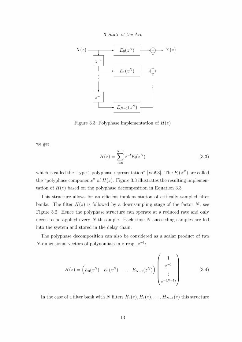
Figure 3.3: Polyphase implementation of H(z)
we get
H(z) =N−1∑l=0
z−lEl(zN) (3.3)
which is called the “type 1 polyphase representation” [Vai93]. The El(zN) are called
the “polyphase components” of H(z). Figure 3.3 illustrates the resulting implemen-
tation of H(z) based on the polyphase decomposition in Equation 3.3.
This structure allows for an efficient implementation of critically sampled filter
banks. The filter H(z) is followed by a downsampling stage of the factor N , see
Figure 3.2. Hence the polyphase structure can operate at a reduced rate and only
needs to be applied every N -th sample. Each time N succeeding samples are fed
into the system and stored in the delay chain.
The polyphase decomposition can also be considered as a scalar product of two
N -dimensional vectors of polynomials in z resp. z−1:
H(z) =(E0(z
N) E1(zN) . . . EN−1(z
N))
1
z−1
...
z−(N−1)
(3.4)
In the case of a filter bank with N filters H0(z), H1(z), . . . , HN−1(z) this structure
13

3 State of the Art
can be extended to
H0(z)
H1(z)...
HN−1(z)
=
E0,0(z
N) E0,1(zN) . . . E0,N−1(z
N)
E1,0(zN) E1,1(z
N) . . . E1,N−1(zN)
......
. . ....
EN−1,0(zN) EN−1,1(z
N) . . . EN−1,N−1(zN)
1
z−1
...
z−(N−1)
= P (zN)
1
z−1
...
z−(N−1)
(3.5)
where the rows of the N×N matrix P (zN) correspond to the polyphase components
of the N filters. P is called the “polyphase matrix” of the filter bank. According
to the Noble identities for multirate systems [Vai93], applying P (zN) followed by
downsampling by N is equivalent to downsampling by N followed by P (z′). Thus
the downsampling required for critically sampled filter banks can be done before
applying the polyphase matrix P .
Similarly, the synthesis filter bank can also be represented by a polyphase matrix
Q. In this case an N -dimensional input is mapped to a 1-dimensional output by
(1 z−1 . . . z−(N−1)
)
Q0,0(zN) Q0,1(z
N) . . . Q0,N−1(zN)
Q1,0(zN) Q1,1(z
N) . . . Q1,N−1(zN)
......
. . ....
QN−1,0(zN) QN−1,1(z
N) . . . QN−1,N−1(zN)
(3.6)
Figure 3.4 illustrates the corresponding polyphase implementation of the analysis
and synthesis filter bank.
In the context of the polyphase decomposition the property of perfect reconstruc-
tion can be described mathematically by the constraint that the synthesis polyphase
matrix has to be the inverse of the analysis polyphase matrix, except for a certain
delay.
14

3 State of the Art
k
k
↓ N
↓ N
z−1
↓ N
z−1
P (z′)
-
-
-
-
-
-
-
-
-
Q(z′)
-?
-
-
↑ N
↑ N
↑ N
z−1
z−1
-
-
-?
?-
?
- -
?
...
X ′(z)
...
X(z) Y0(z′)
Y1(z′)
YN−1(z′)
...
Figure 3.4: Polyphase implementation of a critically sampled filter bank (analysis
and synthesis stage)
3.1.3 Block Transforms
Several types of block transforms are of particular importance in signal processing.
Historically filter banks and transforms were considered as different techniques, but
mathematically this distinction cannot be upheld. Every non-overlapping linear
block transform with N input values and N output values is also a critically sampled
filter bank with N filters of length N . In this case the polyphase matrix only contains
polynomials of order zero. Hence, a block transform can be described by an N ×N
matrix A, and every block or vector x of N samples is transformed into X = Ax.
Usually, in signal processing only orthogonal (resp. unitary) block transforms are
considered, i.e. the inverse of A is the transpose (resp. conjugate transpose) of A.
The orthogonality is useful for three reasons [Mal92]:
• The inverse transform is immediately defined by A, no matrix inversion is
necessary.
• Considering a flow graph of the forward transform, the inverse transform can
be obtained by simply transposing the flow graph, i.e. running it backwards.
• Orthogonal block transforms provide the property of energy conservation,
i.e. ‖X‖ = ‖x‖ where ‖ · ‖ denotes the Euclidean norm. Furthermore, the
reverse is also true: Every energy conserving block transform is orthogonal
15

3 State of the Art
(resp. unitary).
Discrete Fourier Transform
The Discrete Fourier Transform (DFT) of length N is defined by
X(k) =N−1∑l=0
x(l)W klN k = 0, . . . , N − 1 (3.7)
for the forward transform, and
x(l) =1
N
N−1∑k=0
X(k)W−klN l = 0, . . . , N − 1 (3.8)
for the inverse transform, where the primitive N -th root of unity WN is defined by
WN = e−j2π/N
This transform decomposes a sequence of N complex input samples into a weighted
sum of N complex spectral values ranging from 0 up to 2π. Every complex spectral
value contains both a cosine and a sine component. In the case of real input samples
the upper half of the spectral values can be reconstructed from the lower half, and
hence becomes redundant.
Usually a scaling factor of 1/N is used in the inverse DFT, although for energy
conservation a scaling factor of 1/√
N in both the forward and the inverse transforms
would be required.
Fast Fourier Transform
One important advantage of the DFT is the availability of numerous fast implemen-
tations. A direct implementation of an N×N block transform would require O(N2)
operations. The Fast Fourier Transform (FFT), introduced to signal processing in
[CT65], reduces the computational complexity to O(N log N).
The well-known basic principle is the following, see e.g. [OS75]: In case that N is
a power of 2, the radix-2 decimation-in-time approach decomposes the input signal
x(l) into even and odd components, resulting in
X(k) =
N/2−1∑l=0
x(2l)W klN/2 + W k
N
N/2−1∑l=0
x(2l + 1)W klN/2 k = 0, . . . , N − 1 (3.9)
16

3 State of the Art
due to the periodicity of WN/2. Hence the DFT of length N is obtained by N
complex multiplications and additions and two DFTs of length N/2. This process
is repeated recursively, resulting in O(N log(N)) operations.
Several variations of this basic principle are described in literature, such as the
decimation-in-frequency [OS75] and the split-radix approach [DH84]. The FFT plays
an important role in signal processing, because several other block transforms, such
as the Discrete Cosine Transform [Har76], can utilize the FFT for fast algorithms.
Discrete Cosine Transforms
The Discrete Cosine Transform (DCT) decomposes a sequence of N real input sam-
ples into a weighted sum of N real spectral values equally spaced between 0 and π.
Four different types of the DCT are distinguished, according to the classification in
[Wan84], see also [RY90]. They mainly differ in the indexing of time and frequency
axes. At this point, only type II and type IV are described, as they are of particular
interest in signal processing.
DCT of Type II
The DCT of type II (DCTII) is defined by
X(k) = γk
√2
N
N−1∑l=0
x(l) cosk(l + 1
2)π
N, k = 0, . . . , N − 1 (3.10)
with
γ0 = 1/√
2, γk = 1, k = 1, . . . , N − 1
The DCTII is the most widely used type of a DCT. It decomposes the input signal
into N distinct frequency values including a DC value. Especially in image and
video coding a two-dimensional version of the DCTII plays an important role. An
8 × 8 DCTII is used in JPEG image coding [JPEa] and MPEG-1/2 video coding
[MPE93a, MPE00]. The dedicated DC value of the DCTII is especially important
for these applications.
The importance of the DCTII is also due to the asymptotic equivalence to the
Karhunen-Loeve Transform (KLT) for an autoregressive process [ZN77]. For images
and for speech signals an autoregressive process provides a good estimate for the
17

3 State of the Art
statistical correlation properties. Hence the DCTII is a practical alternative to the
optimally decorrelating but signal-dependent KLT.
DCT of Type IV
The DCT of type IV (DCTIV) is defined by
X(k) =
√2
N
N−1∑l=0
x(l) cos(2k + 1)(2l + 1)π
4N, k = 0, . . . , N − 1 (3.11)
Its inverse transform has the same coefficients, and is defined by
x(l) =
√2
N
N−1∑k=0
X(k) cos(2k + 1)(2l + 1)π
4N, l = 0, . . . , N − 1 (3.12)
The applications for the DCTIV are not as wide-spread as for the DCTII, mainly
because of the absence of a dedicated DC value. Nevertheless, the DCTIV is impor-
tant for audio coding applications, because it can be seen as a part of the Modified
Discrete Cosine Transform (MDCT), as will be shown in the following sections.
Based on the DCTIV, such filter banks can be built in a straight-forward way.
3.1.4 The MDCT
The application of non-overlapping block transforms in audio coding, especially in
perceptual audio coding, is not very suitable. The quantization of succeeding blocks
leads to discontinuities in the reconstructed signal, which become easily audible as
so-called blocking artifacts. In frequency domain this can be explained by consider-
ing the frequency responses of the corresponding subband filters. As their frequency
selectivity is inferior to those of filter banks with longer impulse responses, a quanti-
zation of one subband value produces a quantization error covering a larger frequency
range, resulting in an unflat quantization error in time domain.
An early approach to overcome this limitation was to introduce an overlap between
succeeding blocks and apply a windowing function in both the analysis and synthesis
stage [Kra86, Bra87]. This technique allows the reduction of blocking artifacts, but
as the resulting filter bank is no longer critically sampled, the compression efficiency
decreases.
18

3 State of the Art
The Modified Discrete Cosine Transform (MDCT) allows to overcome this lim-
itation and provides both critical sampling and overlapping of blocks. It is based
on a technique called “Time Domain Aliasing Cancellation” (TDAC), introduced in
[PB86, PJB87]. In [PB86] alternating Discrete Cosine Transforms and Discrete Sine
Transforms are used to achieve perfect reconstruction. In [PJB87] a DCTIV based
approach is chosen, allowing to use the same block transform in each block. The
latter is the most commonly used version. It is usually referred to as MDCT,
especially in connection with audio coding applications, such as MPEG-2 AAC
[AAC97]. Nevertheless, other names are also used, e.g. Cosine-Modulated Filter
Bank [RT91, KV91] or Modulated Lapped Transform (MLT) [Mal92]. A similar
approach for lapped transforms focusing on image coding is given by the so-called
Lapped Orthogonal Transform (LOT) [MS88, MS89], providing linear phase filters.
It is also possible to extend the concept of lapped transforms to an overlap of more
than two blocks, e.g. by the Extended Lapped Transform (ELT) [Mal92], or by Low
Delay Filter Banks [SS96, SK00].
The forward MDCT is defined by
X(m) =
√2
N
2N−1∑k=0
w(k)x(k) cos(2k + 1 + N)(2m + 1)π
4N
m = 0, . . . , N − 1
(3.13)
In each block the values x(N), . . . , x(2N − 1) represent the new input samples,
the values x(0), . . . , x(N − 1) represent the input samples of the previous block. In
this way an overlap of 50% is obtained.
The inverse MDCT is defined by
y(k) = w(k)
√2
N
N−1∑m=0
X(m) cos(2k + 1 + N)(2m + 1)π
4N
k = 0, . . . , 2N − 1
(3.14)
The output signal is obtained by adding up the outputs of the inverse MDCT of
two succeeding blocks in their overlapping area.
In both the forward and the inverse transform a window function w is applied in
the time domain. By comparing the output of the overlap-add procedure with the
input signal, a constraint for the window function to achieve perfect reconstruction
19

3 State of the Art
512 1024 1536 2048 2560 30720
0.1
0.2
0.3
0.4
0.5
0.6
0.7
0.8
0.9
1
Samples
Win
dow
Figure 3.5: Sequence of two sine windows with 50% overlap
can be derived. According to [Edl89] the following so-called TDAC condition is
required to assure the time domain aliasing cancellation:
w(k)2 + w(N + k)2 = 1
w(k) = w(2N − 1− k)
}k = 0, . . . , N − 1 (3.15)
A popular example for a window fulfilling this condition is a sine window
w(k) = sin(π
4N(2k + 1))
k = 0, . . . , 2N − 1(3.16)
Figure 3.5 illustrates a sequence of two sine windows for a block length N = 1024.
Before applying the overlap-add of two succeeding blocks during the inverse
MDCT, time domain aliasing occurs. This can be explained by considering the
MDCT as a DCT of length 2N with subsequent sub-sampling in the frequency do-
main [PJB87]. The effect can be regarded as a mirroring of the output of the inverse
MDCT before the overlap-add stage, centered in the middle of each overlapping re-
gion.
20

3 State of the Art
3.1.5 MDCT by Windowing / Time Domain Aliasing and DCTIV
A more explicit, block-oriented approach to the MDCT is possible by considering
the polyphase representation, derived in this section.
Based on the symmetries of the cosine function and the symmetry condition in
Equation 3.15, the following matrix decomposition of the MDCT can be verified:
MDCT =
DCTIV ·
−1
. . .
−1
·
1
. . .
1
1. . .
1
1. . .
1
−1
. . .
−1
·
w(0). . .
w(N − 1)
w(N − 1). . .
w(0)
(3.17)
By means of this decomposition, the process of time domain aliasing is performed
explicitly in time domain, followed by a DCTIV of length N . The processes of time
domain aliasing and windowing are now combined and called “Windowing/TDA” in
the following. By additionally incorporating the delay z−1 of one block of N samples,
21

3 State of the Art
Equation 3.17 results in the following polyphase decomposition of the MDCT:
MDCT = DCTIV ·
−1
. . .
−1
·
w(N2− 1)z−1
. . .
w(0)z−1
w(N2)z−1
. . .
w(N − 1)z−1
w(N − 1). . .
w(N2)
−w(0)
. . .
−w(N2− 1)
(3.18)
This process can also be expressed in the following way: One block of N input
values is processed by two succeeding MDCTs by applying the Windowing/TDA
matrix
WTDA =
w(N − 1). . .
w(N2)
−w(0)
. . .
−w(N2− 1)
w(N2− 1)
. . .
w(0)
w(N2)
. . .
w(N − 1)
(3.19)
and dividing the N intermediate output values between two successive blocks of the
DCTIV.
From the TDAC condition in Equation 3.15 it follows that
w(k)2 + w(N − 1− k)2 = 1 k = 0, . . . ,N
2− 1 (3.20)
Consequently, the Windowing/TDA operation can be described as one stage of
so-called “Givens rotations”, i.e. plane rotations of two-dimensional real values de-
scribed by (cos α − sin α
sin α cos α
)(3.21)
for an angle α. Specifically, the corresponding rotation angles are obtained by
αk = arctanw(k)
w(N − 1− k)k = 0, . . . ,
N
2− 1 (3.22)
22

3 State of the Art
AAAAAAAU�
�������
HH
HHj��
��*
-
-
-
-
AAAAAAAU�
�������
HH
HHj��
��*
-
-
-
-
x(0)
...
x(N−1)
-
-
-
-
-
-
-
-
-
-
-
-
-
-
-
-
DCTIV
DCTIV
DCTIV
DCTIV
DCTIV
DCTIV
AAAAAAAU�
�������
HH
HHj��
��*
-
-
-
-
x(N)
...
x(2N−1)
AAAAAAAU�
�������
HH
HHj��
��*
-
-
-
-
x(0)
...
x(N−1)
x(N)
...
x(2N−1)
X(N−1)
...
X(0)
Figure 3.6: Decomposition of MDCT and inverse MDCT into Windowing/TDA and
DCTIV
For the inverse MDCT the same procedure can be applied in reversed order. The
inverse DCTIV is the DCTIV itself. The Givens rotations applied in the Window-
ing/TDA stage are inverted by applying rotations with negative angles. The whole
process is illustrated in Figure 3.6.
Similar derivations of this decomposition can also be found in [DMP91], [Mal92]
and [SS96]. This decomposition of the MDCT is one main key to the integer ap-
proach in this work.
3.1.6 Low Delay Filter Banks
Besides the MDCT, non-orthogonal versions of modulated filter banks have also
been considered for audio coding applications due to their possibility to reduce
the overall delay or to more closely adapt to psychoacoustic requirements [SS96,
SK00]. These filter banks can be designed by decomposing their structure into a
DCTIV and a cascade of preprocessing steps. In a polyphase representation these
preprocessing steps appear as maximum delay and zero delay matrices and a diagonal
factor matrix.
A forward and an inverse MDCT with N frequency bands introduce a system delay
of 2N−1 samples, see [AGHS99]. By decomposing the MDCT into Windowing/TDA
and DCTIV, as done in Equation 3.18, it can be observed that the DCTIV generates
23

3 State of the Art
AAAAAAAU+
HH
HHj+
-
-
-
-
AAAAAAAU+
HH
HHj+
-
-
-
-
x(0)
...
x(N−1)
-
-
-
-
-
-
-
-
-
-
-
-
-
-
-
-
DCTIV
DCTIV
DCTIV
DCTIV
DCTIV
DCTIV
AAAAAAAU-
HH
HHj-
-
-
-
-
x(N)
...
x(2N−1)
AAAAAAAU-
HH
HHj-
-
-
-
-
x(0)
...
x(N−1)
x(N)
...
x(2N−1)
X(N−1)
...
X(0)
Figure 3.7: Low delay filter bank based on modified MDCT structure
N−1 samples delay and the Windowing/TDA generates additional N samples. The
latter is due to the fact that the Windowing/TDA process makes the current block
dependent on the previous block and vice versa. The basic idea for low delay filter
banks [SS96, SK00] is to allow this dependency in the analysis filter bank only in
forward direction. If the previous block does not depend on the current block, the
Windowing/TDA stage does not introduce any additional delay. An example based
on a slightly modified MDCT structure is illustrated in Figure 3.7. Multiplications
are omitted in this figure for simplicity.
This example leads to a filter bank with perfect reconstruction, a system delay
of N − 1 samples and filter impulse responses of length N + N/2. The impulse
responses can be further extended without introducing additional delay by using
more than N/2 samples from the previous blocks.
A general case of modulated filter banks with arbitrary system delay is derived in
[SK00]. In that approach, the Windowing/TDA stage of MDCT polyphase decom-
position in Equation 3.18 is replaced by a more general structure consisting of the
following building blocks:
24

3 State of the Art
Zero delay matrices
These blocks are defined by
Li(z) := J + diag(li0, . . . , liN/2−1, 0, . . . , 0) · z−1 (3.23)
where li0, . . . , liN/2−1 are real coefficients and
J =
1
. . .
1
(3.24)
The inverse is
L−1i (z) = J − diag(0, . . . , 0, liN/2−1, . . . , l
i0) · z−1 (3.25)
No multiplications with z−1 are required for causality. Thus a cascade of forward
and inverse zero delay matrices does not introduce additional delay. Consequently,
these blocks allow to increase the filter length, but not the system delay.
Maximum delay matrices
These blocks are defined by
Li(z−1) · z−1 (3.26)
The inverse is
L−1i (z−1) · z−1 (3.27)
Both the forward and the inverse block require a multiplication with z−1 for causality.
Thus a cascade of forward and inverse maximum delay matrices introduces a delay
of z−2, resulting in a filter bank with increased system delay.
Diagonal matrix
This building block is defined by
D = diag(d0, . . . , dN−1) (3.28)
with real coefficients d0, . . . , dN−1.
With these basic matrices, the following generalization of the Windowing/TDA
stage is derived in [SK00]:
25

3 State of the Art
-
-
-
-
-
-
-
-
...
X(0)
X(N−1)?
?
-
-
-
-
-
-
-
-
-
-
-
-
-
-
-
DCTIV
DCTIV
-
x(0)
...
x(N−1)
-
-
-
-
-
-
-
-
?
?
?
? ?
?DCTIV
DCTIV
x(0)
...
x(N−1)
x(−N)
...
x(−1)
x(−N−1) -
-
-
-...
x(−2N)
-
-
?
?
?
?
+
+
+
+
+
+
+
+
-
-
DCTIV
-
-
-
-
DCTIV
-
-
-
-
?
?
?
?
-
-
-
-
-
-
-
-
Figure 3.8: Low delay filter bank with two zero delay stages
Fa(z) =ν−1∏j=0
Lµ+ν−1−j(z) ·µ−1∏i=0
(Lµ−1−i(z
−1) · z−1)·D (3.29)
where ν is the number of zero delay matrices and µ is the number of maximum delay
matrices.
The inverse Windowing/TDA stage, with a suitable delay for causality, is
Fs = F−1a (z) = D−1 ·
µ−1∏i=0
(L−1
i (z−1) · z−1) ν−1∏
j=0
L−1µ+j(z) (3.30)
This generalization allows for a wide range of filter banks, including minimum
delay, orthogonal and maximum delay filter banks. The resulting structure of a
low delay filter bank with ν = 2 and µ = 0 can be seen in Figure 3.8. In the
example derived from the MDCT in Figure 3.7 there is ν = 1 and µ = 0. The
MDCT, illustrated in figure 3.6, is also covered by this generalization, featuring an
orthogonal Windowing/TDA stage and ν = µ = 1.
26

3 State of the Art
3.2 Data Compression by Entropy Coding
Entropy coding is an important technique for both perceptual and lossless audio
coding. The goal of entropy coding is to reduce the redundancy when coding signals
with an unequal probability distribution. According to [Sha48], the theoretical limit
of redundancy reduction for a memoryless discrete source is given by the entropy of
M symbols xi with probabilities p(xi)
E =∑
−p(xi) log2(p(xi)) (3.31)
The redundancy is given by the difference of the entropy value to the entropy of a
uniformly distributed source with M symbols:
R = log2 M − E (3.32)
Nowadays, numerous entropy coding methods are established. A large family of
codes follows the principle of variable-size prefix codes [Sal00]. Among them there
are Rice codes, Golomb codes, Shannon-Fano Codes and Huffman codes. The last
one is described in some more detail in the following.
3.2.1 Huffman Coding
Huffman coding [Huf52] is widely used in perceptual audio coding. A Huffman
codebook is assembled using a bottom up strategy, combining the two symbols with
the lowest probabilities to a new composite symbol recursively.
In case all probabilities are negative powers of two, this code can remove all
redundancy. In the general case some redundancy will remain. By combining several
symbols and coding them with a codebook of higher dimension, this redundancy
can be reduced. This limitation results from the integer length of the codewords, as
opposed to the fractional values in the entropy calculations.
3.2.2 Arithmetic Coding
Another popular coding method, Arithmetic Coding, allows to overcome the limi-
tations of integer lengths of codewords. The basic theory was already described in
27

3 State of the Art
Analysis
Filter Bank
Quantization
& Coding
Encoding of
Bitstream
Perceptual
Model
?6
- - -
-
6
-bitstreamaudio in
Figure 3.9: General structure of a monophonic perceptual audio encoder
Decoding of
Bitstream
Inverse
Quantization
Synthesis
Filter Bank- - - -
audio outbitstream
Figure 3.10: General structure of a monophonic perceptual audio decoder
[Sha48]. The realizability within finite precision arithmetic was shown much later,
as described in [MT02]. In an arithmetic coder, instead of a code word for each sym-
bol a sequence of symbols is coded as one fractional number with sufficiently high
precision. In each stage of encoding a symbol, an interval of values is divided into
sub-intervals of widths according to the probabilities. The sub-interval representing
the symbol to be coded becomes the new interval for the next stage. Eventually, an
arbitrary number within the final interval has to be transmitted to the decoder. In
this way no integer number of bits has to be assigned to individual symbols or groups
of symbols, and hence an optimum removal of redundancy is possible theoretically.
3.3 Perceptual Audio Coding
3.3.1 Basic Principles
The majority of perceptual audio coding schemes currently in use follow the general
structure illustrated in Figures 3.9 and 3.10.
28

3 State of the Art
A filter bank is employed to obtain a block by block spectral representation of the
audio signal. The resulting spectral values are quantized and entropy coded. This
process is controlled by a perceptual model which calculates the current masking
threshold of the audio input signal. Based on the masking threshold and the current
bitrate constraints, a quantized representation of the spectral values is determined.
This is usually done iteratively by two nested loops, the rate loop and the distortion
loop, resulting in a trade-off between the inaudibility of quantization errors and the
bitrate constraints. Finally the quantized and entropy coded values and additional
side information are multiplexed into a bitstream.
Early approaches to exploit masking properties of the human ear for speech and
audio coding applications were presented in [BT75, Kra79, SAH79]. However, these
approaches began to receive significant attention from the field of audio coding much
later in [Kra86, Bra87, TLS87].
Filter banks, especially the commonly used MDCT, and entropy coding techniques
have already been described in detail in the previous sections. The other techniques
used in perceptual audio coding are described in more detail in the following.
Perceptual Model
The perceptual model estimates the perceptual masking threshold of the current
audio frame. It is based on the simultaneous masking phenomenon described e.g.
in [ZF90]. Two slightly different effects are considered depending on the tonality of
the masker. Results for tones masked by narrow-band noise and for tones masked
by tones are described there.
Figure 3.11 shows the masking curves introduced by narrow-band noise around
three different frequency values. Around the 1 kHz masker two test tones are shown,
where the left one is audible and the right one is masked.
For tonal maskers similar masking curves occur, but in that case the signal to
mask ratio is much larger. To determine the appropriate masking threshold a tonal-
ity measure can be used to interpolate between the both fashions of simultaneous
masking [Joh88, BJ90].
Additionally, the psychoacoustic phenomenon of temporal masking [ZF90] also
plays an important role. According to this phenomenon transient events mask other
29

3 State of the Art
-100
1020304050607080
20 50 100 200 500 1k 2k 5k 10k 20k
leve
l [dB
]
frequency [Hz]
250 Hz 4 kHz1 kHz
Figure 3.11: Frequency masking of narrow-band noise according to [ZF90]
postt [ms]pret [ms] time
pre-masking
post-masking
simultaneous maskinglevel [dB]
masker
0 100 150 2000-50-100 50
50
3040
100
20
Figure 3.12: Temporal masking according to [ZF90]
events of lower level shortly before and for a longer period after the masking event.
This is illustrated in Figure 3.12. A masker introduces a certain amount of pre- and
post-masking, while the latter is of much longer duration. The illustrated test signal
positioned 50 ms before the onset of the masker is audible, while the test signal 50
ms after the masker is masked.
In contrast to frequency masking, this phenomenon can not be exploited to a such
significant degree in perceptual audio coding. It mainly has to be considered in order
not to exceed the given temporal masking threshold in the block based processing
of the audio codec. Especially the masking threshold before a transient signal can
easily be exceeded, resulting in the so-called “pre-echo phenomenon” [Bra88].
30

3 State of the Art
Quantization
The spectral values are quantized with the intention of hiding a quantization error
just below the masking threshold. Usually, the spectrum is divided into several
frequency bands in line with the Bark scale [ZF90], e.g. half Bark per band. In
each of these bands the same quantizer is applied. A commonly used quantization
method is a power law quantizer. In that approach the spectral values are at first
compressed by a certain power function (e.g. x0.75) and subsequently quantized uni-
formly. This approach was already used by the “OCF” codec introduced in [Bra87]
and is described in detail in [Spo88]. The power law quantizer turns out to be a
good compromise between a uniform quantizer with a constant noise floor and a log-
arithmic quantizer with a constant signal to noise ratio. The power law quantizer
introduces a certain noise shaping within each frequency band, which is beneficial
for more closely meeting the required masking threshold.
3.3.2 Additional Audio Coding Tools
Window Switching
A filter bank with a large number of filters (e.g. an MDCT with 1024 bands) is
advantageous for perceptual coding of tonal signals in order to exploit the frequency
masking. On the other hand, for transient signal portions the same configuration
can cause severe pre-echo artifacts. In this case the quantization error spreading
over the whole length of the analysis window can easily violate the pre-masking
threshold.
A successful method to meet these varying requirements is presented in [Edl89]. It
is shown that the shape of the MDCT window function can be changed in each block
individually while maintaining the perfect reconstruction property. Furthermore,
using a window function with a reduced range of overlap, the succeeding block can
switch to an MDCT with a lower number of bands, covering a smaller range of
time domain samples. In this way a trade-off between frequency resolution and time
resolution can be made dynamically according to the signal characteristics.
Based on the decomposition of the MDCT described in Section 3.1.5, the process
of window switching can be described in a very modular way. In order to switch to
31

3 State of the Art
x(0)
...
x(N−1)
x(N)
...
x(2N−1)
x(2N)
...
x(3N−1)
x(3N)
...
x(4N−1)
x(0)
...
x(N−1)
x(N)
...
x(2N−1)
x(2N)
...
x(3N−1)
x(3N)
...
x(4N−1)
X(N−1)
...
X(0)
X(2N−1)
...
X(N)
X(3N−1)
...
X(2N)
AAAAAAAU�
�������
HH
HHj��
��*
-
-
-
-
HH
HHj��
��*-
-
HH
HHj��
��*-
-
HH
HHj��
��*-
-H
HHHj�
���*
-
-H
HHHj�
���*
-
-
AAAAAAAU�
�������
HHHHj����*
-
-
-
-
-
-
-
-
DCTIV
DCTIV
DCTIV
DCTIV
DCTIV
DCTIV
DCTIV
DCTIV
-
-
-
-
-
-
-
-
-
-
-
-
-
-
-
-
-
-
-
-
-
-
-
-
-
-
-
-
-
-
-
-
DCTIV
DCTIV
DCTIV
DCTIV
DCTIV
DCTIV
DCTIV
DCTIV
AAAAAAAU�
�������
HH
HHj��
��*
-
-
-
-
HH
HHj��
��*-
-
HH
HHj��
��*-
-
HH
HHj��
��*-
-H
HHHj�
���*
-
-H
HHHj�
���*
-
-
AAAAAAAU�
�������
HHHHj����*
-
-
-
-
-
-
-
-
Figure 3.13: Window switching for MDCT and inverse MDCT decomposed into
Windowing/TDA and DCTIV
a lower transform length, the range of values covered by the Windowing/TDA stage
has to be reduced. The succeeding block can then switch to a DCTIV of shorter
length. The range covered by the Windowing/TDA stage is always centered around
the border of two DCTIV blocks. Figure 3.13 illustrates a situation where switching
between a long block and four short blocks is applied.
Temporal Noise Shaping
By means of the technique of entropy coding in spectral domain a high coding
gain can be achieved especially for tonal signals. For transient parts of the signal
the coding gain is low due to the flat spectrum of transient signals. As set out in
32

3 State of the Art
[HJ96, HJ97b], this flatness can be exploited by applying linear prediction in the
frequency domain. A forward-adaptive linear predictive coding (LPC) approach
[JN84] is applied, utilizing the autocorrelation function of the spectral values and
the Levinson-Durbin recursion. The required filter order typically ranges between 4
and 12. In [HJ96] two alternatives are described. One uses an open loop predictor,
the other uses a closed loop predictor. The first alternative is called “Temporal
Noise Shaping” (TNS). The quantization after the prediction leads to an adaption
of the resulting quantization noise to the temporal structure of the audio signal and
therefore prevents pre-echoes in perceptual audio coders. In contrast to the Window
Switching technique, TNS also delivers an improvement for pitch-based signals such
as speech. TNS in combination with filter banks such as the MDCT can be seen
as a continuously signal-adaptive filter bank [HJ97a], allowing control over the time
and frequency structure of the quantization noise.
Joint Stereo Coding
Two widely used joint stereo coding techniques are described in [HEB92]: Intensity
Stereo Coding and M/S Stereo Coding.
Intensity Stereo Coding is used as a tool for irrelevancy reduction at lower bitrates.
In the high frequency range only one channel is transmitted, in addition to the energy
envelope of both channels. This technique allows to reduce the bitrate for stereo
signals, but it can also lead to a loss of spatial information.
M/S Stereo Coding aims for high quality coding at higher bitrates. For this
technique a matrixing can be applied in order to code sum and difference instead of
the left and the right channel. This allows to exploit inter-channel redundancy and
it shapes the quantization noise spatially to avoid stereo unmasking effects.
Perceptual Noise Substitution
The Perceptual Noise Substitution (PNS) technique is a parametric coding tech-
nique for noise-like signal portions. It was introduced for high-quality audio coding
in [Sch96, HS98]. It allows to efficiently code noise-like frequency bands by just
transmitting the total energy of this band and synthesizing the spectral values based
on a noise generator in the decoder.
33

3 State of the Art
3.3.3 MPEG-1 Layer-3 and MPEG-2/4 AAC
Nowadays numerous perceptual audio coding schemes following the basic principles
described in Section 3.3.1 are available. As examples, the coding schemes MPEG-1
Layer-3 (MP3) [MPE93b] and MPEG-2 AAC [AAC97] shall be described in some
detail here. A comprehensive description of both coding schemes can also be found
in [Bra99].
MPEG-1 Layer-3
In this codec a hybrid filter bank is used, consisting of a 32-band polyphase filter
bank cascaded with an 18-band MDCT, resulting in 576 frequency bands. A method
to reduce aliasing effects of cascaded filter banks [Edl92] is included. The window
switching technique is used, allowing 3 times a 6-band MDCT instead of the 18-band
MDCT for transient signal portions. The quantization and coding stage utilizes a
non-uniform quantizer and Huffman coding. In order to determine a perceptually
optimum quantization result within a fixed bitrate, usually two nested loops (rate
loop and distortion loop) are applied. To allow for a local variation of the bitrate
within the constraint of a constant bitrate, a bit-reservoir technique is applied. For
stereo signals Intensity coding and M/S coding can be employed.
MPEG-2 AAC
MPEG-2 Advanced Audio Coding (AAC) can be seen as a further development
of MPEG-1 Layer-3. It is based on similar technical principles. Nevertheless, a
backwards compatibility was not considered in order to get the best improvement in
coding efficiency. Figure 3.14 shows a block diagram of an MPEG-2 AAC encoder.
In the following the most important improvements compared to MPEG-1 Layer-3
are described. An MDCT with a high frequency resolution of 1024 bands is used
instead of a hybrid filter bank. The block switching technique allows to switch to
eight times 128 bands for transient signals. Additionally the TNS tool can be used.
The joint stereo coding tools Intensity and M/S coding have become more flexible
in that they can be switched on or off for each scale factor band individually. An
optional prediction tool can further improve the coding efficiency for very tonal
34

3 State of the Art
Input time signal
PerceptualModel
GainControl
FilterBank
Prediction
Rate/DistortionControl Process
M/S
ScaleFactors
Quantizer
NoiselessCoding
BitstreamMultiplex
13818-7Coded AudioStream
TNS
Intensity/Coupling
Legend
Data Control
QuantizedSpectrumof Prev.Frame
Figure 3.14: Block diagram of MPEG-2 AAC encoder
35

3 State of the Art
g
g
Analysis
Filter Bank
Quantization
& Coding
Inverse
Quantization- - -audio in
Quantization
& Coding
Quantization
& Coding
Inverse
Quantization
Bitstream
Multiplex
�?
?
- -
-
�
--
--
-
- Perceptual
Model-
-
bit-
stream
-
-
Figure 3.15: Basic principle of scalable perceptual audio coder
signals by applying a backward adaptive predictor on each frequency value. Finally,
the Huffman coding is made more flexible.
3.4 Scalable Perceptual Audio Coding
3.4.1 Scalable Enhancement of AAC
Scalable Coding, also called “Hierarchical Coding”, allows to arrange the coded
signal in a hierarchical way. Usually the bitstream is divided into so-called “Layers”.
The more layers are decoded, the higher is the signal quality and the overall bitrate.
Every enhancement layer provides additional information for decoding to higher
quality.
The concept of scalability was introduced to perceptual audio coding in [BG94].
In that publication the scalability was obtained by a time-domain approach, using
complete encoding and decoding stages and calculation of the time-domain error
after each stage. In [GB95] a frequency-domain approach is presented. It allows
to encode several layers in frequency domain by starting with a coarse quantiza-
tion of the spectral values and refining them for the enhancement layers. Figure
3.15 illustrates the basic structure of a three-layer system utilizing several stages
of quantization and inverse quantization in frequency domain. An evaluation of
different scalable approaches can be found in [Gri01].
36

3 State of the Art
The frequency domain approach is also adopted as a scalable extension of AAC in
MPEG-4 [MPE01, Gri97]. Additionally, this scalable codec allows other codecs such
as CELP or TwinVQ as core codecs in the first layer. Furthermore, a mono-stereo
scalability is possible, allowing a mono signal to be enhanced to a stereo signal.
A comprehensive description of the MPEG-4 AAC Scalable codec can be found in
[Gri99].
In [ARR01] a modification of the structure in Figure 3.15 is proposed, considering
the compander property of the non-uniform quantizer and performing all quanti-
zation stages in the compressed domain. Rudimentarily, this approach is already
mentioned in [GB95].
3.4.2 Fine-Grain Scalable Audio Coding
The concept of fine-grain scalable audio coding by bitsliced arithmetic coding
(BSAC) was introduced for audio coding in [PKKS97] and is standardized as a
part of MPEG-4 [MPE01].
In this context, BSAC plays the role of an alternative lossless coding kernel for
MPEG-4 AAC, utilizing the MDCT and applying a perceptually controlled bandwise
quantization to the spectral values. The main difference between BSAC and the
standard AAC lossless coding kernel is that the quantized values are not Huffman
coded, but arithmetically coded in bitslices. This allows a fine grain scalability
by omitting some of the lower bitslices while maintaining a compression efficiency
comparable to that of the Huffman coding approach.
3.5 Lossless Audio Coding
Lossless audio coding can be achieved either by predictive coding or by transform
coding. The basic principles and some representative systems will be described
in the following. The theory behind both approaches is described in [JN84], also
showing that the theoretically possible coding gain for stationary random signals is
equal in both approaches.
37

3 State of the Art
m m-
-6
Predictor
-
6
Predictor
--
�
e(n)x(n) x(n)
− +
Figure 3.16: Basic principle of predictive coding
3.5.1 Prediction-Based Lossless Audio Coding
Predictive coding is a widely adopted technique for lossless audio coding. Early
adoptions of this technique to lossless audio coding can be found in [Moo79] and
[SH86]. In [Moo79] first and second order difference values of the audio samples are
coded. In [SH86] this concept is extended by using a set of integer coefficient filters.
The basic principle of predictive coding is to predict the value of the current sample
based on the values of previous samples, and only encode the remaining difference
value. In the decoder the same predictor is used to reconstruct the original values.
This is illustrated in Figure 3.16.
In [JN84] the theoretical background of obtaining an optimum linear prediction
filter with a minimum mean squared error is described. Based on the autocorrelation
function of the signal, the optimum linear predictor of length N is described by
the Wiener-Hopf equations. The Levinson-Durbin algorithm provides an efficient
recursive algorithm for finding this optimum prediction filter.
Several lossless audio coding approaches using this linear predictive coding (LPC)
technique have been published [CT93, CCR93, BOvdVvdK96, Rob94]. Alternative
approaches use IIR prediction filters instead of FIR prediction filters [CG96, CLS97,
GCS+99] or backward adaptive prediction [Ang97]. Furthermore, the linear predic-
tion concept can also be applied successfully to correlated stereo channels, resulting
in a stereo prediction as an alternative to mid-side coding [CT93, Lie02, Ghi03].
In recent years numerous predictive lossless audio codecs have been developed
and published on the internet as freeware, e.g. Shorten [Rob94, Sof], LPAC [Lie04],
Monkey’s Audio [Ash], FLAC [Coa], OptimFROG [Ghi]. Several articles provide
performance evaluations of some of these codecs, e.g. [HS01a]. Especially on the
internet, some frequently updated comparisons can be found, e.g. [Spe04, Hei04].
These comparisons use several Audio CDs with popular music as input signals. They
38

3 State of the Art
report compression ratios of 55% resp. 53% of the original size, depending on the
selection of the input signals.
3.5.2 Transform-Based Lossless Audio Coding
An approach for using transform coding for lossless audio coding has been presented
in [PLN97]. In this approach the DCT is used to transform the audio signal block
by block. A quantization is applied to the spectral values to allow efficient entropy
coding of the spectral values. This quantization introduces an error into the signal
representation which is coded additionally in time domain. The basic structure in
this approach is motivated by the idea mentioned in [CG96] to use a lossy coding
algorithm and additionally code the error signal to achieve lossless coding.
A similar approach was presented in [KSB97, KSB99]. In that approach the
MDCT is used instead of the DCT.
Both approaches have the same drawback: The transforms used produce floating
point values even for integer input values. The number of possible output values
increases considerably compared to the number of possible input values. One rea-
son for this effect is the energy compaction property of the transform, resulting in
a higher range of possible spectral values compared to the range of input values.
Another reason is given by the actual coefficients of the transform. As they stem
from trigonometric functions, they are usually irrational numbers. Thus the spectral
values consist of linear combinations of these irrational numbers. Due to these prop-
erties of the underlying transform it seems impossible to directly encode all possible
spectral values in an efficient way. Hence a quantization is necessary to achieve a
reduction of data rate. By applying a quantization, the perfect reconstruction prop-
erty of the transform is destroyed. Consequently, for lossless audio coding either the
quantization has to be fine enough to allow neglecting the resulting error, or the
error signal has to be coded additionally in time domain.
One major goal of this work is to eliminate this drawback. This will be achieved
by introducing a quantization in the transform without destroying the perfect re-
construction property.
39

3 State of the Art
Lossless
Coder
Perceptual
Decoder
Perceptual
Coder-
-
?
?
Scalable Encoder
-
Perceptual
Decoder
Lossless
Decoder
Scalable Decoder
-
-
-
+
lossless
audio
perceptually
coded audio
?
-audio in perceptually
coded
bitstream
lossless
enhancement
bitstream
Figure 3.17: Principle of scalable perceptual and lossless coding in time domain
3.6 Scalable Perceptual and Lossless Audio Coding
In principle, a perceptual codec can be extended to a scalable perceptual and lossless
system by including the perceptual decoder in the encoder, calculating the error sig-
nal in time domain and additionally coding this residual signal. This basic idea has
already been mentioned in [CG96]. Figure 3.17 illustrates the general structure of
such an approach. A system utilizing this approach has been presented in [MIJM00]
using an MPEG-4 audio codec as a perceptual core codec.
A drawback of these approaches, as was already mentioned in [CG96], is the
bit-exact conformance of the core codec. In order to assure lossless decoding, a bit-
exact operation of the perceptual core codec has to be demanded. Usually this is not
the case in specifications of perceptual codecs, see e.g. [MPE01]. Due to different
decoder implementations, slightly different waveform outputs can occur. This does
usually not affect the perceptual quality of the different outputs, but it precludes
a realization of this scalable system based on different available implementations of
the underlying perceptual decoder.
One goal of this work is to eliminate this drawback by providing an architecture
for scalable perceptual and lossless coding in frequency domain.
40

3 State of the Art
3.7 Integer-to-Integer Transforms
3.7.1 Ladder Network and Lifting Scheme
Usually, orthogonal block transforms are decomposed into Givens rotations(cos α − sin α
sin α cos α
)
in order to obtain fast algorithms. While these basic building blocks are mathemat-
ically invertible by just applying a rotation with the corresponding negative angle,
this inversion can in general not be done exactly within a limited precision of the in-
put values and the coefficients. Especially for lossless coding of integer input values,
integer output values are desired, while the invertibility (or perfect reconstruction
property) should be maintained.
This issue can be solved by using a structure called “lifting scheme” or “lad-
der network”. The “ladder network” technique was introduced into digital signal
processing in [Cro72] and [MS73]. In these publications it was used as an implemen-
tation method for digital filters. In [BE92] this technique is applied to transform
coding to maintain perfect reconstruction in the presence of quantization. Both a
general solution for 2×2 matrices with determinant 1, and some examples for higher
dimensions are presented. In [THK95] ladder networks are applied to two-band FIR
filter banks.
A very similar approach is introduced in [DS98, CDSY98], using the name “lifting
scheme”. In these publications decompositions of 2 × 2 matrices are utilized in the
context of wavelet transforms.
In more recent publications the term “lifting scheme” has become more frequently
used than the term “ladder network”. In the following the author will also use the
term “lifting scheme”.
The basic building blocks of the lifting scheme are called “lifting steps”. They
have the general structure
La =
(1 0
a 1
)(3.33)
with a real value a called “lifting coefficient”, or the transpose of this matrix. The
41

3 State of the Art
lifting step La maps two value (x1, x2) to
La(x1, x2) = (x1, x2 + ax1) (3.34)
The inverse lifting step is given by
L−1a = L−a =
(1 0
−a 1
)(3.35)
In case of integer input values (x1, x2) a rounding function [·] can be included into
the lifting step La in order to obtain integer output values. The resulting integer
lifting step is given by
La,[·](x1, x2) = (x1, x2 + [ax1]) (3.36)
Despite of the rounding function, this integer lifting step can still be inverted. The
inverse integer lifting step is given by
L−1a,[·](x1, x2) = (x1, x2 − [ax1]) (3.37)
If the rounding function [·] is odd symmetric, the inverse integer lifting step can also
be expressed by
L−1a,[·] = L−a,[·] (3.38)
Overall, every lifting step can be approximated by an integer mapping without
sacrificing the invertibility. Hence, every matrix that can be decomposed into lifting
steps can be converted into an invertible integer approximation with this technique.
A lifting step decomposition for a 2× 2 matrix(a b
c d
)with b 6= 0 and determinant 1 is described in [BE92] by(
a b
c d
)=
(1 0
(d− 1)/b 1
)(1 b
0 1
)(1 0
(a− 1)/b 1
)(3.39)
Based on this general decomposition for 2 × 2 matrices the following lifting de-
composition for Givens rotations can easily be obtained:
(cos α − sin α
sin α cos α
)=
(1 cos α−1
sin α
0 1
)(1 0
sin α 1
)(1 cos α−1
sin α
0 1
)(3.40)
42

3 State of the Art
@@
@@
@@R��
��
���
-
-
-
-
cos α
cos α
+
+
− sin α
sin α
Figure 3.18: Givens rotation
-6 6
-
-
-
-?
+
+
+cos α−1
sin αsin α cos α−1
sin α
Figure 3.19: Givens rotation by three lifting steps
-6 6
-
-
-
-?
+
+
+− cos α−1
sin α− sin α − cos α−1
sin α
Figure 3.20: Inverse Givens rotation by three lifting steps
Figure 3.18 illustrates the direct application of a Givens rotation. Figures 3.19
and 3.20 show the forward and inverse lifting decompositions.
By converting the three lifting steps in Equation 3.40 into integer lifting steps, an
integer approximation of this Givens rotation is obtained, called “integer rotation” in
the following. This integer rotation can be inverted without introducing an error by
applying the inverse lifting steps in reverse order using the same rounding function.
Every transform that can be decomposed into Givens rotations can utilize this
decomposition and can consequently be approximated by an invertible integer trans-
form.
43

3 State of the Art
3.7.2 Integer Transforms
In recent years lifting-based filter banks and transforms have widely been discussed
and adopted in the context of image coding. The image coding standard JPEG2000
[JPEb] adopts a lifting based Discrete Wavelet Transform, in line with the develop-
ment in [DS98, CDSY98].
As was mentioned above, every transform, that can be decomposed into Givens
rotations, can be approximated by a lossless integer transform using the lifting
scheme. Concerning transforms focusing on image coding this technique has al-
ready been presented several times. In [KS98] an 8-point lossless Discrete Cosine
Transform (DCT) is obtained. In [KS00] an 8-point lossless Lapped Orthogonal
Transform (LOT) is described. In [LT01, Tra00b, Tra00a] this technique is further
refined to get fast multiplierless approximations of DCT and LOT used in image
coding. Similarly, an approximation of the Fast Fourier Transform (FFT) has been
proposed in [OCN01].
In [WVVY01] an integer DCT is used to remove inter-channel redundancy of a
perceptually coded multichannel audio signal. This is done in a lossless way after
the quantization of the MDCT values of the respective channels.
44

4 New Integer Transforms for Audio
Coding
4.1 The Integer Modified Discrete Cosine Transform
As shown in Section 3.1.5, the MDCT can be decomposed into a Windowing/TDA
stage consisting of Givens rotations and the DCTIV. This stage can be implemented
with lifting steps by defining the lifting coefficients
csk =w(N − 1− k)− 1
w(k), sk = w(k) (4.1)
based on the window function w(k), k = 0, . . . , 2N − 1. Thus the Windowing/TDA
stage can be performed by utilizing N/2 integer rotations. Figure 4.1 illustrates the
structure of the resulting Integer Windowing/TDA stage.
The DCTIV can also be decomposed into Givens rotations by utilizing a fast
O(N log N) algorithm. A possible decomposition is described in [Wan84]. In [SBE92]
another decomposition of the DCTIV into Givens rotations is described implicitly by
presenting a fast algorithm for the MDCT. Another very common fast algorithm for
the DCTIV utilizes the FFT in combination with two stages of Givens rotations, see
[Mal92].
All these decompositions have in common that, overall, the MDCT is completely
decomposed into Givens rotations. Hence, the lifting scheme can be applied to get
an invertible integer approximation of the MDCT, called Integer Modified Discrete
Cosine Transform (IntMDCT) in the following. This approach was first presented
by the author in [GSKB01].
Here it should be noted that fast algorithms for the DCTIV usually comprise a
45

4 New Integer Transforms for Audio Coding
-
-
-
-
x(0)
...
x(N/2−1)
x(N/2)
...
x(N−1)
?
6
6
?
? ?
?
6
6
?
?
·cs0
[·]
[·]
·s0
·cs0
[·]?
6?
·csN/2−1
[·]
[·]
·sN/2−1
·csN/2−1
[·]?
6?
?
. . .
Figure 4.1: Integer Windowing/TDA using lifting
large number of trivial sum-difference butterflies(1 −1
1 1
)(4.2)
A direct implementation of these butterflies, as usually done in fast algorithms,
would be invertible, but the energy of the signals would increase by a factor of 2
for each butterfly. In order to avoid this for the IntMDCT, these butterflies are
normalized and implemented as integer rotations with an angle of π/4. The lifting
implementation assures an energy conservation, apart from the introduced quanti-
zation error. Hence the IntMDCT provides a certain kind of energy conservation.
Due to the overlapping structure, an energy conservation on a block by block basis,
like the one described by Parseval’s Theorem, can not be achieved. Energy can
be distributed unequally between two succeeding blocks. Nevertheless, the average
energy per block is maintained because during the complete process only integer
rotations are applied. Despite this energy conservation, it has to be considered that
the range of possible integer spectral values is higher than the range of the integer
input values. This is due to the energy compaction property of the transform. The
maximum possible value can be estimated by considering the ideal case that the
46

4 New Integer Transforms for Audio Coding
−160
−140
−120
−100
−80
−60
−40
−20
0 2 4 6 8 10 12 14 16 18 20 22
leve
l [dB
]
frequency [kHz]
IntMDCTMDCT
Figure 4.2: IntMDCT and MDCT spectra of sine 1kHz -20dBFS
energy of a full-scale sinusoidal signal is compacted to exactly one spectral value.
The IntMDCT inherits most of the favorable properties of the MDCT, including
the overlapping structure and critical sampling by means of Time Domain Aliasing
Cancellation. When evaluating the frequency selectivity of the IntMDCT, it has to
be noted that non-linearities are inherent in the lifting steps due to the quantization.
Consequently, it is not sufficient to consider the IntMDCT in the way of conventional
linear FIR filters by computing frequency responses. The frequency selectivity of the
IntMDCT is therefore estimated by comparing the IntMDCT spectrum of certain
input signals with the MDCT spectrum.
Figure 4.2 shows both IntMDCT and MDCT magnitude spectra of a 1 kHz sine
wave with a level of -20dBFS. Both transforms use a resolution of 1024 spectral
values and a sine window.
As can be seen from Figure 4.2, the inherent non-linearities become apparent
as an internal ‘noise floor’ at a level of around -110dBFS. Since the absolute level
47

4 New Integer Transforms for Audio Coding
−160
−140
−120
−100
−80
−60
−40
−20
0 2 4 6 8 10 12 14 16 18 20 22
leve
l [dB
]
frequency [kHz]
IntMDCTMDCT
difference
Figure 4.3: IntMDCT and MDCT spectra of Carl Orff’s Carmina Burana
of these rounding errors stays approximately constant for most part of the input
signal, the frequency selectivity of the IntMDCT depends on the input signal level.
For audio signals containing significant energy in each frequency band, however,
the added distortion can be neglected and the IntMDCT closely approximates the
MDCT. Figure 4.3 depicts absolute IntMDCT, MDCT and difference values for Carl
Orff’s Carmina Burana (track 64 of SQAM [SQA88], see Table 7.1). The difference
values are not correlated with the spectral values and assume a constant order of
magnitude over the whole spectrum.
4.2 Integer Low Delay Filter Banks
The low delay filter banks described in Section 3.1.6 can be seen as a generalization
of the MDCT with arbitrary system delay. In this section it will be shown that a
lifting-based integer approximation is also possible in this general case.
48

4 New Integer Transforms for Audio Coding
Looking at the general decomposition of the Windowing/TDA stage in the ana-
lysis filter bank in Section 3.1.6, it can be observed that the basic building blocks
of zero delay matrices and maximum delay matrices already consist of lifting steps.
Hence, the only task remaining to obtain a complete decomposition into lifting
steps is the decomposition of the N ×N diagonal matrix in Equation 3.28:
D = diag(d0, . . . , dN−1)
Without loss of generality it can be assumed that the determinant of D is 1. To
obtain a lifting decomposition of D, the following decomposition of a 2× 2 diagonal
matrix with determinant 1 is used:
(d 0
0 d−1
)=
(−1 0
d−1 1
)(1 −d
0 1
)(0 1
1 d−1
)(4.3)
Similar to the lifting decomposition of Givens rotations, this decomposition can
be regarded as a special case of the 3-step lifting decomposition of 2 × 2 matrices
presented in Equation 3.39. In [DS98] a similar lifting decomposition of 2×2 diagonal
matrices is accomplished by four lifting steps.
The diagonal matrix D can be decomposed into N − 1 2 × 2 diagonal matrices
with a determinant of 1 by starting with
D = diag(d0, d−10 , 1, . . . , 1) · diag(1, d0 · d1, d2, . . . , dN−1) (4.4)
and applying the same decomposition recursively to the (N − 1) × (N − 1) matrix
diag(d0·d1, d2, . . . , dN−1) .
In this way the low delay filter bank described in Section 3.1.6 can be completely
decomposed into lifting steps, as long as the minor restriction is met that the deter-
minant of the diagonal matrix D is one.
This result is a generalization of the result published by the author in [GS02].
In that paper the lifting decomposition was obtained under the restriction that
di = 1/dN−1−i for i = 0, . . . , N/2 − 1. This has been shown to be equivalent to
constraining the prototype windows in the analysis and synthesis filter bank to be
identical except for a sign. However such a restriction is not severe, as it holds in
most practical applications.
49

4 New Integer Transforms for Audio Coding
4.3 Improved IntMDCT Using Multi-Dimensional
Lifting
4.3.1 Introduction
As described in the previous sections, integer transforms can be obtained by decom-
posing the transform into Givens rotations and applying the lifting scheme or ladder
network to each Givens rotation. These integer rotations introduce a rounding error
in each step. For succeeding stages of integer rotations the rounding error accumu-
lates. The resulting difference between the spectral values of the original transform
and the spectral values of the corresponding integer transform is called “approx-
imation error” in the following. This approximation error becomes a drawback,
especially for long transforms of e.g. 1024 spectral values, as used in audio coding
applications. Specifically for the high frequency range, where audio signals usually
contain a rather small amount of energy, the approximation error can be larger than
the actual signal and becomes the main limiting factor for lossless coding efficiency.
So the main design objective for improved integer transforms is the reduction of
the approximation error. Besides that, the computational complexity should also
be considered. The current approach of applying the lifting scheme to each Givens
rotation, including trivial sum-difference butterflies, increases the computational
complexity, compared to the original non-integer version of the transform, by a
factor of about 2.
Some publications [BE92], [KS98], [HS01b], [WSY03], mostly focusing on lossless
image coding, propose a reduction of the resulting approximation error by a general-
ized lifting decomposition. In these generalizations the processing of more than two
values is proposed. The corresponding N ×N matrix is decomposed into unit upper
and lower triangular matrices. In order to implement a lossless integer approxima-
tion of this decomposition, a maximum of N−1 rounding operations is introduced for
each triangular matrix. So the total number of rounding operations can be reduced
compared to the conventional lifting approach. In [BE92] and [HS01b] triangular
matrix decompositions using 2N − 1 or N + 1 rounding operations are reported.
Unfortunately, these approaches cannot simply be applied to long transforms used
in audio coding because the resulting algorithm has a considerable computational
50

4 New Integer Transforms for Audio Coding
complexity (O(N2)) compared to fast, rotation-based algorithms (O(N log N)). Fur-
thermore, the dynamic range of the values in the triangular matrices can increase
too much to allow a practical implementation.
The approach presented in [WSY03] uses block matrices to recursively obtain a
triangular matrix decomposition. While the new approach presented in the following
is based on similar block matrices, no recursion is necessary here. This approach
was published by the author in [GYS03, GYSH04].
4.3.2 From Classic to Multi-Dimensional Lifting
Based on the general lifting decomposition of 2 × 2 matrices in Equation 3.39 the
following decomposition has been derived in Equation 4.3:(d 0
0 d−1
)=
(−1 0
d−1 1
)(1 −d
0 1
)(0 1
1 d−1
)
This decomposition provides the basic idea for the new approach put forward in
this section. The equation still holds when all values are replaced by n×n matrices.
Thus, for any invertible n × n matrix T and for the n × n identity matrix In the
following decomposition of 2n× 2n block matrices is possible:
(T 0
0 T−1
)=
(−In 0
T−1 In
)(In −T
0 In
)(0 In
In T−1
)(4.5)
Apart from some simple operations, such as permutations or multiplication by
−1, all three blocks of this decomposition have the following general structure:(In 0
A In
)(4.6)
with an n× n matrix A.
To this 2n × 2n block matrix a generalized lifting scheme can be applied, called
“Multi-Dimensional Lifting” or “MDL” in the following. Similar to the conventional
lifting scheme with 2× 2 matrices presented in Section 3.7.1, these 2n× 2n matrices
can be used for invertible integer approximations of the transform T in the following
way: The first half of the integer input values are processed by the matrix A, rounded
to integer values, and finally added to the second half of the values.
51

4 New Integer Transforms for Audio Coding
-
-
-
-
-
A
[·] [·][·][·]
-
-
-
?
?
?
?
?
?
?
?
+
+
+
+
...
x(0)
x(n−1)
x(n)
x(2n−1)
...
...
x(0)
x(n−1)
x′(n)
x′(2n−1)
...
Figure 4.4: Forward step for multi-dimensional lifting with rounding ([·])
The inverse of the block matrix is given by(In 0
A In
)−1
=
(In 0
−A In
)(4.7)
In this way, the process can be inverted without any error by simply applying the
same matrix A and the same rounding, and subtracting the resulting values instead
of adding them. As the first half of the values is not modified in the forward step,
they are still available for the inverse operation. Figures 4.4 and 4.5 illustrate the
forward and inverse step. No special restrictions apply to the matrix A, e.g. it does
not necessarily have to be invertible.
4.3.3 IntMDCT by Multi-Dimensional Lifting
In the IntMDCT approach presented in Section 4.1, both the Windowing/TDA stage
and the DCTIV are decomposed into Givens rotations and approximated by integer
rotations. The number of Givens rotations necessary for the DCTIV is O(N log N)
for a transform of length N . The Windowing/TDA stage consists of only N/2 Givens
52

4 New Integer Transforms for Audio Coding
-
-
-
-
-
A
[·] [·][·][·]
-
-
-
?
?
?
?
?
?
?
?
-
-
-
-
...
x(0)
x(n−1)
x′(n)
x′(2n−1)
...
...
x(0)
x(n−1)
x(n)
x(2n−1)
...
Figure 4.5: Inverse step for multi-dimensional lifting with rounding
rotations, resulting in 3N/2 rounding steps. Consequently, concerning transform
lengths used in audio coding applications, e.g. 1024, the main contribution to the
approximation error results from the integer approximation of the DCTIV block.
Based on the multi-dimensional lifting approach the number of rounding opera-
tions necessary for the integer approximation of the DCTIV can be reduced to O(N),
as shown in the following.
4.3.4 The Stereo IntMDCT
The most straight-forward way of using the multi-dimensional lifting approach for
the calculation of the IntMDCT is to apply a DCTIV to two blocks of input signals
simultaneously. These blocks can either be two subsequent blocks of the input
signal or correspond to the left and the right channel of a stereo input signal. The
decomposition in Equation 4.5 is applied to the DCTIV matrix. Since the inverse of
53

4 New Integer Transforms for Audio Coding
a DCTIV is again the DCTIV, the decomposition in Equation 4.5 becomes:(DCTIV 0
0 DCTIV
)=(
−IN 0
DCTIV IN
)(IN −DCTIV
0 IN
)(0 IN
IN DCTIV
)(4.8)
The steps of permutations and multiplications with −1 can be isolated to separate
block matrices: (DCTIV 0
0 DCTIV
)=(
−IN 0
0 IN
)(IN 0
DCTIV IN
)(IN −DCTIV
0 IN
)(IN 0
DCTIV IN
)(0 IN
IN 0
)(4.9)
Thus, apart from permutations and multiplications with −1, the application of the
DCTIV to two blocks of signals can be performed using three multi-dimensional
lifting steps: (IN 0
DCTIV IN
)(IN −DCTIV
0 IN
)(IN 0
DCTIV IN
)(4.10)
This process is illustrated for a stereo signal with left channel xL and right chan-
nel xR in Figure 4.6, including the rounding operations required for the integer
approximation. The inverse process is illustrated in Figure 4.7.
With this approach, two DCTIV transforms of length N can be implemented in
an invertible integer fashion with only 3N rounding steps, i.e. 3N/2 rounding steps
per transform.
The DCTIV used in the three multi-dimensional lifting steps can be of an arbitrary
implementation, such as floating-point or fixed-point based, and does not need to be
invertible. It just has to be performed in the same way in the forward and inverse
IntMDCT. The overall computational complexity is about 1.5 times larger than in
case of a non-integer implementation of the two DCTIV transforms. Compared to
the approach in Section 4.1 based on the conventional lifting scheme, a significant
complexity reduction is achieved. This is due to the fact that this implementation,
being about twice as complex as a conventional DCTIV, has to handle the trivial sum-
difference butterflies by integer rotations in order to guarantee energy conservation,
as described in Section 4.1.
54

4 New Integer Transforms for Audio Coding
? ? ? ? ? ? ? ?
-
-
-
-
-
-
-
-
DCTIV
?
?
?
?
DCTIV
?
[·] [·]
?
[·]
?
[·]
?
DCTIV
6 6 6 6
[·] [·] [·] [·]
[·] [·] [·] [·]
6
6
6
6
+
+
+
+
+
+
+
+
-
-
-
-
...
xR(0)
xR(N−1)
xL(0)
xL(N−1)
...
...
−XL(0)
−XL(N−1)
XR(0)
XR(N−1)
...
Figure 4.6: Invertible integer approximation of two blocks of DCTIV by three multi-
dimensional lifting steps
? ? ? ? ? ? ? ?
-
-
-
-
-
-
-
-
DCTIV
?
?
?
?
DCTIV
?
[·] [·]
?
[·]
?
[·]
?
DCTIV
6 6 6 6
[·] [·] [·] [·]
[·] [·] [·] [·]
6
6
6
6
-
-
-
-
-
-
-
-
+
+
+
+
...
−XL(0)
−XL(N−1)
XR(0)
XR(N−1)
...
...
xR(0)
xR(N−1)
xL(0)
xL(N−1)
...
Figure 4.7: Inverse of integer approximation of two blocks of DCTIV by three multi-
dimensional lifting steps
55

4 New Integer Transforms for Audio Coding
4.3.5 The Mono IntMDCT
The Stereo IntMDCT approach requires the simultaneous calculation of two DCTIV
transforms, e.g. by calculating the DCTIV of two subsequent blocks or by calculating
the DCTIV of left and right channel simultaneously. While the first alternative
introduces an additional delay of one block, the second alternative only is possible
for stereo signals. If neither delay nor stereo processing is desired, multi-dimensional
lifting is still viable, but some additional stages of Givens rotations become necessary.
A DCTIV of length N (see Equation 3.11)
DCT(N)IV =
(√2
Ncos
(2k + 1)(2l + 1)π
4N
)k,l=0,...,N−1
(4.11)
can be decomposed into two DCTIV of length N/2 and some additional processing
steps. In the following, such a decomposition is described. A similar decomposition
can also be found in [ZBL01].
Define the N ×N matrix L by(Lk,k Lk,N−1−k
LN−1−k,k LN−1−k,N−1−k
)=(
cos(2k+14N
π) − sin(2k+14N
π)
− sin(2k+14N
π) − cos(2k+14N
π)
)k = 0, . . . , N/2− 1 (4.12)
Lk,l = 0 else
the N ×N matrix M by
M =1√2
(IN/2 IN/2
−IN/2 IN/2
)(4.13)
and the N ×N permutation matrices P and Q by
P4k,4k = P4k+1,4k+1 = P4k+2,4k+3 = P4k+3,4k+2 = 1 (4.14)
k = 0, . . . , N/4− 1
Pk,l = 0 else
i.e. every second pair of values is swapped, and
Qk,2k = QN/2+k,2k+1 = 1 k = 0, . . . , N/2− 1 (4.15)
Qk,l = 0 else
56

4 New Integer Transforms for Audio Coding
-
-
-
DCTIV
-
-
-
-
-
-
-
DCTIV
-
-
-
-
-CCCCCCCCCW�
���������
CCCCCCCCCW�
���������
CCCCCCCCCW�
���������
CCCCCCCCCW�
���������
-CCCCCCCCCCCCCCCW�
���������������
CCCCCCCCCCCW�
�����������
CCCCCCCCW�
��������
AAAAU�
����...
x(0)
x(N−1)
...
X(0)
X(N−1)
Figure 4.8: DCTIV of length N by two DCTIV of length N/2 and two stages of Givens
rotations
i.e. the values with even indices are mapped to the first half, and the values with
odd indices are mapped to the second half.
With these matrices, the DCTIV of length N can be decomposed into
DCT(N)IV = L
(DCT
(N/2)IV 0
0 DCT(N/2)IV
)MQP (4.16)
Figure 4.8 illustrates the basic structure of this decomposition.
The two DCTIV of length N/2 can be decomposed into three multi-dimensional
lifting steps of length N/2 using Equation 4.8. The matrices L and M can both be
considered as N/2 Givens rotations. Instead of decomposing M into 3N/2 lifting
steps, a more efficient approach with a smaller number of rounding operations can
be applied here. The matrix M can be implemented using the multi-dimensional
lifting steps (IN/2 0
−12IN/2 IN/2
)(IN/2 IN/2
0 IN/2
)(4.17)
The scaling factors√
2 and 1/√
2, which are necessary for normalization, can be
57

4 New Integer Transforms for Audio Coding
handled by the DCTIV stage. Overall, the following decomposition can be obtained:(DCT
(N/2)IV 0
0 DCT(N/2)IV
)M
= 1√2
(DCT
(N/2)IV DCT
(N/2)IV
−DCT(N/2)IV DCT
(N/2)IV
)
=
(0 1√
2DCT
(N/2)IV
−√
2DCT(N/2)IV 0
)(12IN/2 −1
2IN/2
IN/2 IN/2
)
=
(IN/2
1√2DCT
(N/2)IV
0 IN/2
)(IN/2 0
−√
2DCT(N/2)IV IN/2
)(IN/2
1√2DCT
(N/2)IV
0 IN/2
)
·
(IN/2 −1
2IN/2
0 IN/2
)(IN/2 0
IN/2 IN/2
)(4.18)
The lifting implementation of matrices L and M can be combined with the
DCTIV stage in order to further reduce the overall number of rounding operations.
This is done by merging the remaining N/2 rounding operations regarding M , and
N/2 of the 3N/2 rounding operations regarding L with the rounding operations in
the DCTIV stage. This merging of rounding operations is based on the following
property of multi-dimensional lifting matrices:(In 0
A In
)(In 0
B In
)=
(In 0
A + B In
)(4.19)
Overall only 5N/2 rounding operations are necessary for this invertible integer ap-
proximation of the DCTIV of length N . Including the windowing stage, the total
number of rounding operations for this IntMDCT is 4N , i.e. 4 rounding operations
per sample.
So far, only the multi-dimensional lifting decompositon of block matrices of the
form (T 0
0 T−1
)given in Equation 4.5 was utilized in this section. Nevertheless, it is also possible to
decompose other block matrices into multi-dimensional lifting steps. For example,
the following decomposition can be used to implement the combination of one stage
58

4 New Integer Transforms for Audio Coding
of normalized sum-difference butterflies and two blocks of DCTIV by three stages of
multi-dimensional lifting:
1√2
(IN IN
−IN IN
)(DCTIV 0
0 DCTIV
)=
(1√2DCTIV
1√2DCTIV
− 1√2DCTIV
1√2DCTIV
)=(
IN 0
IN −√
2DCTIV IN
)(IN
1√2DCTIV
0 IN
)(IN 0
IN −√
2DCTIV IN
)(4.20)
Such a decomposition provides a way of simultaneously calculating the IntMDCT
spectra of a stereo signal and the mid-side matrixing without increasing the number
of rounding operations compared to the Stereo IntMDCT processing.
Furthermore, the existence of this decomposition raises the question, whether the
DCTIV matrix itself can be decomposed into three multi-dimensional lifting steps
without the need for additional pre- or postprocessing steps. In the course of this
research several decompositions were developed by the author, but it was not pos-
sible to find fast algorithms for these decompositions. Additionally, the dynamic
range of the resulting coefficients tends to increase for larger block lengths.
4.3.6 Approximation Accuracy
The approximation accuracy of the IntMDCT based on multi-dimensional lifting is
evaluated by applying the transform to the audio material used for the lossless audio
coding activities of the ISO MPEG group [MPE02]. The audio material consists of
recordings by the New York Symphonic Ensemble and jazz recordings, see Table
7.2. Evaluation is done for both 48 kHz / 16 bit and 96 kHz / 24 bit. Only the left
channels of the signals are used in this evaluation. The performance of the different
transforms is evaluated comparing mean squared error (MSE), maximum absolute
error and an entropy estimate, calculated by∑
k log2(2|yk|+1), where yk represents
the integer spectral values. In the subsequent evaluation, the number of instructions
value reflects the number of additions and multiplications.
For the IntMDCT, a transform length of 1024 frequency bands is used. Table 4.1
shows the results for the conventional lifting based IntMDCT, the multi-dimensional
lifting based Mono IntMDCT, and, as a reference, the rounded MDCT, which does
not allow lossless operation. Here the approximation error is calculated by building
59

4 New Integer Transforms for Audio Coding
Lifting based MDL based Rounded MDCT
IntMDCT IntMDCT (not lossless)
Rounding
operations
per sample 22.5 4 1
Instructions
per sample 45 32 20
MSE (in LSB) 1.97 0.48 0
max. abs. Error 8 4 0
Entropy estimate
48 kHz 16 bit 1.180 · 108 1.166 · 108 1.160 · 108
Entropy estimate
96 kHz 24 bit 4.145 · 108 4.125 · 108 4.113 · 108
Table 4.1: Comparison of conventional lifting-based IntMDCT, multi-dimensional
lifting (MDL) based Mono IntMDCT and rounded MDCT (not lossless)
the difference between the IntMDCT values and the rounded MDCT values. The
resulting MSE and maximum absolute error values are similar for both audio input
formats, thus only the overall values are displayed.
It can be observed that the approximation error is largely reduced by the multi-
dimensional lifting approach, and the estimated entropy comes close to the theoret-
ical limit given by the rounded MDCT.
The multi-dimensional lifting approach leads to a substantial reduction in round-
ing error compared to the approach presented in Section 4.1. Using this approach,
only 3 or 4 rounding steps per sample are required, irrespective of the transform
length. This is particularly advantageous for large transform lengths (e.g. 1024)
used in audio coding applications, compared to e.g. 22 rounding steps per sample
for the previous approach. With the reduction of the rounding error an improved
compression performance in the context of lossless audio coding applications can be
expected.
60

4 New Integer Transforms for Audio Coding
nn [·] -
- �
z−1
6
- -
��H(z)
X(z) Y (z)
E(z)
−−
Figure 4.9: Spectral shaping of quantization error
4.4 Improved IntMDCT by Noise Shaping
With the multi-dimensional lifting based IntMDCT in Section 4.3, the necessary
number of rounding operations required for the DCTIV can be reduced to 1.5 oper-
ations per sample. This is the same number of rounding operations as necessary for
the Windowing/TDA stage, which makes a further investigation into the rounding
process during the Windowing/TDA stage interesting. In this section noise shaping
is introduced in some rounding stages to obtain a frequency dependent behavior of
the approximation error.
The technique of noise shaping with regard to quantization of time-domain signals
is described in [GC89]. The basic structure is illustrated in Figure 4.9. In each stage,
the quantization error is calculated and an error feedback including a filter H(z) is
utilized. In the z domain the system can be described by
E(z) = Y (z)− (X(z)− E(z)z−1H(z)) (4.21)
which is equal to
Y (z) = X(z) + E(z)(1− z−1H(z)) (4.22)
Hence the resulting quantization error is filtered by
1− z−1H(z) (4.23)
With this filter the spectral shape of the quantization noise can be modified. In
A/D conversion this is utilized by applying a high-pass filter, and consequently
shifting the quantization noise to the high frequency range. Especially for high
sampling rates (e.g. 96 kHz) a large, inaudible frequency range can be utilized for
61

4 New Integer Transforms for Audio Coding
-
-
-
-
x(0)
...
x(N/2−1)
x(N/2)
...
x(N−1)
?
6
6
?
??
?
6
6
?
?
·cs0
. . .
[·]
[·]
·s0
. . .
·cs0
. . .
[·]?
6?
·csN/2−1
[·]
[·]
·sN/2−1
·csN/2−1
[·]?
6?
?
Figure 4.10: Reordered Integer Windowing/TDA using lifting
this purpose. The simplest version of noise shaping is given by H(z) = 1, resulting
in the high-pass filter 1− z−1.
In the context of integer transforms for lossless audio coding the desired shape of
the noise floor is exactly the opposite. Especially in the high frequency range, where
audio signals usually have a very low amount of energy, the noise floor becomes a
drawback for lossless coding efficiency and should be as low as possible. On the
other hand, in the lower frequency range audio signals usually have a very high
energy compared to the noise floor introduced by the integer transform. Hence a
slight increase of the noise floor is not expected to impair the coding efficiency in
this frequency range. Overall, a lowpass shape of the quantization noise is desirable
in the context of integer transforms.
In order to see, how the noise shaping technique can be applied in the context of
the IntMDCT, the Integer Windowing/TDA stage illustrated in Figure 4.1 has to be
reordered first. This is possible without changing the output results, as illustrated in
Figure 4.10. This reordered structure consists of three stages where N/2 succeeding
floating-point values are rounded and added to N/2 succeeding integer values. In
this context the noise shaping technique can be applied, as illustrated in Figure 4.11.
62

4 New Integer Transforms for Audio Coding
-
-
-
-
x(0)
...
x(N/2−1)
x(N/2)
...
x(N−1)
?
6
6
?
??
?
6
6
?
?
·cs0
. . .
[·]/NoiseShaping
[·]/NoiseShaping
·s0
. . .
·cs0
. . .
[·]/NoiseShaping?
6?
·csN/2−1
·sN/2−1
·csN/2−1
?6
?
?
Figure 4.11: Integer Windowing/TDA with noise shaping
The noise shaping can also be applied in some stages of the Integer DCTIV based on
multi-dimensional lifting. Generally, application of this technique is useful as long
as the signal, to which the quantization error is added, can be regarded as a time
domain signal. Concerning the Stereo IntMDCT (see Section 4.3), this is the case
for the first of three multi-dimensional lifting steps. This can be seen by considering
the quantization error signals δ1, δ2 and δ3 added in the corresponding rounding
stages of the three multi-dimensional lifting steps in Figure 4.6. At the output this
results in the error signals
−DCTIV(δ1)− δ2 (4.24)
in the upper part and
δ1 + DCTIV(−DCTIV(δ1)− δ2) + δ3 = −DCTIV(δ2) + δ3 (4.25)
in the lower part.
As the influence of δ1 cancels out in the lower part, δ1 only influences the time
domain input of the upper part, and hence noise shaping can be applied in the first
lifting step. In the second lifting step the situation is ambivalent, as δ2 influences
both time domain and frequency domain. Further studies would be required to
63

4 New Integer Transforms for Audio Coding
0 100 200 300 400 500 600 700 800 900 10000
0.1
0.2
0.3
0.4
0.5
0.6
0.7
0.8
0.9
1
spectral value
mea
n sq
uare
d er
ror
noise shapingno noise shaping
Figure 4.12: Mean squared approximation error of Stereo IntMDCT per spectral
value, with noise shaping (gray line) and without noise shaping (black
line)
determine the usefulness of noise shaping in this lifting step. Finally, in the third
lifting step of the Stereo IntMDCT noise shaping is clearly not possible.
Figure 4.12 illustrates the approximation error of the Stereo IntMDCT, both with
and without noise shaping. Without noise shaping an approximately white approx-
imation error can be observed, whereas it is shaped towards the lower frequency
range when noise shaping is applied.
Table 4.2 lists the approximation error and entropy estimates both with and
without noise shaping, evaluated for the MPEG Lossless [MPE02] test material at
48 kHz / 16 bit. As a reference, the entropy estimate of the rounded MDCT values
are also calculated as a theoretical limit.
64

4 New Integer Transforms for Audio Coding
No noise Noise Rounded MDCT
shaping shaping (not lossless)
MSE 0.38 0.54 0
max. abs. Error 4 9 0
Entropy estimate 2.305 · 108 2.304 · 108 2.297 · 108
Table 4.2: Comparison of Stereo IntMDCT with and without noise shaping, and
rounded MDCT (not lossless). Input format: 48 kHz / 16 bit
It can be observed that, while the approximation error increases when noise shap-
ing is applied, the value for the entropy estimate is slightly reduced. Hence for
typical audio signals, a slight improvement regarding the compression ratio can be
expected by using the noise shaping technique.
65

5 New Audio Coding Schemes and
Applications Based on Integer
Transforms
5.1 Lossless Audio Coding Based on IntMDCT
5.1.1 Basic Concept
The IntMDCT provides a good spectral representation of an audio signal while
staying in integer domain. When applied to tonal parts of an audio signal, this
results in a good energy compaction. So an efficient lossless coding scheme can
be built by simply combining the IntMDCT with an entropy coding scheme. This
coding scheme should suit the properties of the IntMDCT values. In contrast to
entropy coding schemes for transform coding described in [AAC97] and [KSB97],
the spectral values to be coded are not dynamically scaled to certain quantization
step sizes. So a wide range of values has to be considered. In the following a possible
entropy coding scheme is described.
5.1.2 Entropy Coding Scheme
In order to adapt to different statistics of the spectral values, the spectral domain
is divided into bands derived from the Bark scale. One possible decomposition is
described in [AAC97] using approximately two bands per Bark. A different Huffman
codebook can be used for each band. The entropy coding scheme is implemented
using eight Huffman codebooks with lengths ranging between one and 16384 code
words, combined with stacked coding. Values exceeding the maximum codebook
66

5 New Audio Coding Schemes and Applications Based on Integer Transforms
value are coded by stacked coding, as described in [KSB97].
5.1.3 First Results
Using the described entropy coding scheme, first results concerning the compression
efficiency are obtained using the following setup: For the IntMDCT a frame length
of 1024 samples and a sine window are used. The sound material used for testing
comes from the SQAM compact disc [SQA88], listed in Table 7.1. These items have
shown to be very critical for perceptual audio coding and have often been used as a
reference for lossless audio coding. Encoding all tracks, an average data rate of 4.9
bit per sample is achieved. This is in the same range of efficiency as ‘conventional’
coding schemes, as compared in [HS01a].
For a realistic estimation for lossless coding efficiency of other audio signals it has
to be considered that the SQAM items contain a large amount of zero samples at the
beginning and at the end of each track. Therefore, frames which only contain zero
samples are omitted in the following results. If the whole set of signals is encoded
with zero frames omitted the average data rate increases to 5.6 bit per sample.
In Figure 5.1 the average bitrates for individual SQAM items are presented. Espe-
cially for the artificial signals (tracks 3-7) and some of the single instruments items
(tracks 8-43) a high coding gain is achieved. The worst case item for this compres-
sion scheme is Carl Orff’s Carmina Burana (track 64) with an average bitrate of 9.1
bit per sample. This complex item contains choir and orchestra and has a very rich
spectrum, see Figure 4.3.
Apart from the average data rate, it is also important to know which maximum
data rate usually occurs. In these test results the highest peak data rates measured
were 14.9 bit per sample for track 31 (cymbal) and track 65 (orchestra, R. Strauss),
and 13.9 bit per sample for track 27 (castanets). In all these items the peak data
rates occur in transient parts of the signal.
These results for lossless audio coding based on IntMDCT were first published by
the author in [GSKB01].
67

5 New Audio Coding Schemes and Applications Based on Integer Transforms
5 10 15 20 25 30 35 40 45 50 55 60 65 700
1
2
3
4
5
6
7
8
9
10EBU SQAM
bit p
er s
ampl
e
track #
Figure 5.1: Average bitrates for lossless coding of SQAM items, zero frames omitted
68

5 New Audio Coding Schemes and Applications Based on Integer Transforms
5.1.4 Additional Coding Tools
Several additional coding tools for perceptual audio coding, described in Section
3.3.2, can be adapted to lossless operation in order to enhance the performance of
an IntMDCT based lossless audio coding scheme:
Window Switching
The window switching technique described in Section 3.3.2 can be applied to the
IntMDCT in the same way as done for the MDCT. In the context of lossless audio
coding this technique can be used to dynamically adapt between high frequency
resolution and high time resolution. This allows to achieve a high coding gain also
for non-stationary signal portions.
Linear Prediction in Frequency Domain
As pointed out in Section 3.3.2, linear prediction in frequency domain can be used
advantageously in the context of perceptual audio coding, especially for transient
signals. Both an open loop and a closed loop prediction can be used. This principle
can also be applied to lossless audio coding. In this context the second alternative is
more appropriate because closed loop prediction allows perfect reconstruction of the
input signal. When applying this technique to the IntMDCT spectrum, a rounding
to integer values has to be applied to each output value of the prediction filter
in order to stay in the integer domain. By using the inverse filter and the same
rounding, the original spectrum can be reconstructed perfectly.
Joint Stereo Coding
To exploit the redundancy between two channels, mid/side coding can be applied
in a lossless way by applying an integer rotation with an angle of π/4. The integer
rotation has the advantage of energy conservation. The alternative of applying sum
and difference to the IntMDCT values would also be lossless, but it would increase
the energy by a factor of 2, and hence increase the bitrate.
The usage of joint stereo coding can be switched on and off for each band, as done
in MPEG-2 AAC [AAC97]. Other rotation angles may also be considered in order
69

5 New Audio Coding Schemes and Applications Based on Integer Transforms
to reduce redundancy between two channels more flexibly. Clearly, this would also
require more side information than for mid/side coding.
For multichannel signals the lossless redundancy reduction scheme based on the
Integer Discrete Cosine Transform described in Section 3.7.2 may be considered.
5.2 Scalable Lossless Enhancement of a Perceptual
Audio Coder
5.2.1 Introduction
In section 3.4.1 a scalable enhancement of AAC is described, providing a base layer
and several enhancement layer bitstreams. Each enhancement layer gradually in-
creases the bitrate and the achieved perceptual quality.
Here, a scalable system, which enhances a perceptually coded base layer bitstream
by means of a lossless enhancement layer bitstream, is presented. So lossless decod-
ing can be achieved when decoding both layers. In contrast to the time domain
approach described in Section 3.6, however, there is no need to fully decode the
base layer in order to perform entropy coding of a time domain residual signal.
By virtue of the IntMDCT, coding of the lossless enhancement layer is performed
completely in the frequency domain.
5.2.2 Concept of Scalable System
Based on its perfect reconstruction property and the close approximation of the
MDCT, the IntMDCT allows to build a scalable lossless enhancement of MDCT-
based perceptual audio coding schemes. Figure 5.2 illustrates the concept of the
proposed scalable architecture which consists of a conventional perceptual base layer
coder and a lossless enhancement coder based on the IntMDCT.
Encoder
The structure of the encoder is an extension of the general structure of a perceptual
audio coding scheme, described in Section 3.3.1. In addition to the usual MDCT
70

5 New Audio Coding Schemes and Applications Based on Integer Transforms
MDCTaudioin
PerceptualModel
Quantization& Coding
Encoding ofbitstream
perceptuallycodedbitstream
perceptualaudio
Decoding ofbitstream
InverseQuantization
InverseMDCT
IntMDCT
InverseQuantization& Rounding
EntropyCoding
losslessenhancementbitstream
-
perceptuallycodedbitstream
losslessenhancementbitstream
EntropyDecoding
InverseIntMDCT
losslessaudio
+
ENCODER
DECODER
Rounding
Figure 5.2: Perceptual audio coding scheme (solid lines) and scalable lossless en-
hancement (dashed lines)
71

5 New Audio Coding Schemes and Applications Based on Integer Transforms
spectrum, the IntMDCT spectrum is calculated. For the lossless enhancement, the
difference between the IntMDCT spectrum and the inverse quantized MDCT spec-
trum is calculated. These difference values are entropy coded and transmitted by
means of the lossless enhancement bitstream. This produces both a lossy (per-
ceptually coded) bitstream and a lossless enhancement bitstream which carries the
information necessary to exactly reconstruct the input signal.
Decoder
In the decoder the quantized MDCT spectrum is reconstructed from the percep-
tually coded bitstream. By applying the inverse MDCT, the perceptually coded
audio signal can be obtained. If the enhancement bitstream is decoded, the residual
IntMDCT spectrum can be obtained in addition. By adding the inverse quantized
MDCT spectrum, the IntMDCT spectrum is reconstructed. Finally the inverse
IntMDCT is applied to get the losslessly coded audio signal.
A simplified version of this coding scheme may be considered by reusing the
IntMDCT for the perceptual part instead of the MDCT. In this way the calculation
of only one transform would be required in the encoder.
5.2.3 Bit-Exact Reconstruction of Original Signal
When using a scalable coder that is based on the coding of a time domain residual
signal, as described in Section 3.6, the reconstruction precision of the lossy base
layer coder becomes critical for achieving an overall lossless reconstruction. Specif-
ically, an implementation with a very high numeric precision is necessary in order
to approximate the “exact” output of the decoding process, which is by definition
a floating-point process. Even with a very high numerical precision in the base
layer decoder, however, an occasional bit-difference between different decoder im-
plementations can not be avoided. In order to design a truly lossless system, the
IntMDCT-based solution circumvents this problem. It only requires the inverse
quantization process of the perceptual decoder to be specified exactly with inte-
ger output. Then the remaining steps for lossless decoding can be performed in
the integer domain, and especially an exactly specified inverse IntMDCT assures a
bit-exact processing by definition. Consequently, a lossless reconstruction can be
72

5 New Audio Coding Schemes and Applications Based on Integer Transforms
achieved without having to rely on floating-point precision.
5.2.4 Codebook Selection without Side Information
The magnitude of the residual IntMDCT spectrum depends on the accuracy of quan-
tization. Thus, for an efficient entropy coding of the residual signal it is useful to use
a selection of entropy codebooks. In the MPEG-2 Advanced Audio Coding (AAC)
[AAC97] scheme, described in Section 3.3.3, the spectral coefficients are grouped
into scalefactor bands and the spectral values are weighted by an amplification fac-
tor derived from the corresponding scalefactor. Since a non-uniform quantizer is
applied to the weighted spectral values, the magnitude of residual values not only
depends on the scalefactors, but also on the quantized values themselves. Both the
scalefactors and quantized spectral values are transmitted in the AAC bitstream and
can be utilized for the choice of appropriate codebooks for the residual spectrum
without transmitting any additional side information. The choice of the appropriate
codebook is made individually for each spectral value depending on the width of the
quantization interval applied in the perceptual coding part.
5.2.5 Window Switching
As described in Section 5.1, the window switching technique can also be applied to
the IntMDCT. In the context of the scalable perceptual and lossless system described
in this section, this can be achieved by using the window switching decisions made
by the perceptual core coder in the IntMDCT of the lossless enhancement.
5.2.6 Results for Scalable Perceptual and Lossless Audio Coding
The system shown in Figure 5.2 has been implemented and evaluated using MPEG-2
AAC as the MDCT based perceptual base layer coding scheme. For first results, a
simplified version of AAC with MDCT and window switching, but no further coding
tools, is used. The lossless enhancement bitstream employs 24 Huffman codebooks
with lengths ranging between one and 4096 code words. Each spectral value can use
the appropriate codebook without the need of additional side information.
73

5 New Audio Coding Schemes and Applications Based on Integer Transforms
AAC (kbps/channel) 64 80 96
AAC (bits/sample) 1.5 1.8 2.2
Enhancement (bits/sample) 4.2 4.0 3.8
Total (bits/sample) 5.7 5.8 6.0
Table 5.1: Bitrate results for SQAM CD coded with scalable lossless coding scheme
Table 5.1 summarizes bitrate results for the entire SQAM CD [SQA88] (see also
Table 7.1), including all zero samples.
The AAC encoder uses constant bitrates resulting in variable bitrates for the
lossless enhancement bitstream. The total bitrate of this scalable system is slightly
increased compared to the lossless system described in Section 5.1. One reason for
this scalable overhead could be the constant bitrate of the AAC codec which is
a very inefficient way of representing the zero parts of the tracks. Another reason
could be the focus of AAC to produce a perceptually equivalent representation of the
audio signal rather than simply reducing the energy of the error signal. Finally, the
necessity to round the inverse quantized AAC spectral values to integer values before
subtracting them from the IntMDCT spectral values leads to a certain reduction of
the lossless coding efficiency of this scalable system.
5.3 Scalable Lossless Enhancement Using the
Structure of MPEG-4 AAC Scalable
In the previous section the concept of scalable lossless enhancement of AAC in
frequency domain has been presented. This approach was first published by the
author in [GHKB02].
The codec described in this section is a further development of this concept. It
is completely based on the structure of the MPEG-4 AAC Scalable codec [MPE01].
By utilizing the IntMDCT, this codec is extended to a lossless operation with only a
minor extension of the bitstream syntax. Furthermore, scalability of sampling rate
and reconstruction word length is supported.
74

5 New Audio Coding Schemes and Applications Based on Integer Transforms
MDCT Quantization& Coding
BitstreamMultiplex
Integer InverseQuantization
LSB Shift& CodingIntMDCT
audioin
-
TNS M/S
IntegerTNS
IntegerM/S
Figure 5.3: Encoder for scalable lossless enhancement of AAC
HuffmanDecoding
InverseQuantization
InverseMDCT
InverseIntMDCT
Decoding& LSB Shift
Integer InverseQuantization
percep-tuallycodedaudio
+ losslessaudio
Bit-stream
Demulti-plex
M/S TNS
IntegerM/S
IntegerTNS
Figure 5.4: Decoder for scalable lossless enhancement of AAC
This scalable lossless audio coding system was published by the author in [GSH+03]
and proposed to the ISO MPEG committee in [GDHS02, Gei03b, Gei03a] in response
to the Call for Proposals on MPEG-4 Lossless Audio Coding [MPE02].
5.3.1 Scalable System Based on AAC
In addition to the general concept of scalable lossless enhancement in frequency
domain described in Section 5.2, the coding scheme presented in this section contains
several AAC-specific refinements. Figures 5.3 and 5.4 show the encoder and decoder
block structure of this codec. To get an efficient lossless extension of AAC, especially
the coding tools Mid/Side-Coding (M/S) and Temporal Noise Shaping (TNS) are
considered and implemented in a lossless integer fashion.
75

5 New Audio Coding Schemes and Applications Based on Integer Transforms
In the following, the important blocks of this codec are described in detail.
Inverse Quantization to Integer Values
One crucial point for the lossless operation of the system is the inverse quantization
and rounding process in the decoder. According to [MPE01], the inverse quantized
and rescaled values depend on the quantized value xquant and the scale factor sf ,
and are calculated by:
xinvquant = sign(xquant) ∗ |xquant|4/3
gain = 20.25∗(sf−SF OFFSET ) (5.1)
xrescal = xinvquant ∗ gain
These values xrescal are rounded to integer in order to generate the difference values
for the lossless enhancement layer. To make these operations reliable and inde-
pendent of the specific implementation, the codec uses fixed integer look-up tables.
According to [MPE01], the maximum allowed absolute amplitude for xquant is 8191.
Thus, for one scalefactor an integer table with 8192 values is needed. Such a table
is, however, not needed for all possible scale factor values. When increasing the
scale factor by 4, the corresponding gain is scaled by a factor of 2. Hence tables are
needed for only four specific scale factor values, i.e. sf0, sf0 + 1, sf0 + 2, sf0 + 3.
With these four tables, all the inverse quantized integer values can be derived by
applying bit shift operations.
Encoding of Lossless Enhancement Layer Values with LSB Shift
The coding of the lossless enhancement layer values can be achieved by completely
reusing the bitstream syntax of the MPEG-4 AAC Scalable codec [MPE01], de-
scribed in Section 3.4.1. Only one additional element is introduced in order to
enable efficient coding of large spectral values. To achieve an appropriate compres-
sion of the integer difference values of the lossless enhancement layer, an entropy
coding scheme has to be applied. The noiseless coding tool of AAC can be reused
for this task with only small modifications. Compared to the coarsely quantized
spectral values of AAC, the integer values for the lossless enhancement layer encom-
pass a much larger range. To apply the AAC noiseless coding tool appropriately, the
76

5 New Audio Coding Schemes and Applications Based on Integer Transforms
absolute values of the integer difference values are divided into LSB and MSB values
by applying a certain number of bit shift operations. The MSB values are coded
using the AAC noiseless coding tool, and the LSB values are coded as PCM values
according to the number of bit shifts. The number of bit shifts can be chosen for
each scale factor band individually. To encode the number of bit shifts for each scale
factor band, the scale factor coding mechanism of AAC is reused. In the decoder the
integer difference values can be reconstructed based on the MSB and LSB values.
This technique allows for a flexible adaptation to the statistical characteristics of
the integer values. It therefore achieves efficient entropy coding without the need
for additional, larger Huffman codebooks. Concerning the bitstream syntax of the
lossless enhancement layer, the bitstream syntax of AAC can be reused by adding
the functionality of coding the LSB values.
Compliance with AAC Coding Tools
The lossless enhancement is compliant with the AAC coding tools Block Switching
and Window Shape Adaptation, TNS, M/S and PNS, described in Section 3.3.2.
Thus, no restrictions apply to the usage of these tools in the lossy core. Furthermore,
they can even be applied advantageously to the lossless enhancement layer. In detail,
the lossless enhancement deals with those tools in the following way:
Block Switching and Window Shape
The IntMDCT in the lossless enhancement layer can use the same window shape and
window sequence as the AAC coder, so that the lossless enhancement can simply
follow the block switching and window shape decisions of the lossy core coder.
Temporal Noise Shaping (TNS)
The TNS tool in AAC modifies the MDCT spectrum by applying linear prediction
filters before quantization. Consequently, the difference between the IntMDCT val-
ues of the lossless enhancement layer and the quantized MDCT values of the AAC
core layer increases. The TNS tool can, however, also be applied to the IntMDCT
values in a lossless way by using the same prediction filter and applying a rounding
77

5 New Audio Coding Schemes and Applications Based on Integer Transforms
to integer values to each output value of the prediction filter. As the MDCT and
the IntMDCT values only differ by a small approximation error, the filtered spectral
values only differ by the filtered approximation error and the additional rounding
error. In the decoder, the original IntMDCT spectrum is reconstructed by using the
inverse filter and the same rounding. This lossless version of the TNS filter works
as closed loop prediction and provides a redundancy reduction for transient signals,
as stated in Section 5.1.
Mid/Side Coding (M/S)
The M/S coding tool in AAC modifies some scale factor bands of the MDCT spec-
trum by calculating the sum and difference of left and right channel spectral values.
The lossless enhancement layer can follow the M/S decisions of the lossy AAC core
coder and can apply M/S coding in a lossless way. This is done by applying an
integer rotation with an angle of π/4, based on the lifting scheme. Thereby the
energy is conserved and the original IntMDCT values can be reconstructed in the
decoder, as also mentioned in Section 5.1.
Perceptual Noise Substitution (PNS)
The lossless enhancement is compliant with the PNS tool described in Section 3.3.2.
This is done in the same way as for the AAC Scalable codec: In the scale factor
bands where PNS is switched on, the inverse quantized spectral values are assumed
to be zero for calculating the difference values for the enhancement layer.
5.3.2 Lossless-Only Mode
The system can also operate in a lossless-only mode. In this mode no AAC core
layer is used and the IntMDCT spectral values are coded within one layer. The
bitstream is identical to an AAC bitstream, extended by the additional LSB coding
described above. The coding tools Block Switching and Window Shape Adaption,
TNS and M/S can be used in a lossless way for the purpose of further redundancy
reduction.
78

5 New Audio Coding Schemes and Applications Based on Integer Transforms
AAC (kbps/channel) 0 64 80 96
AAC (bits/sample) 0 1.5 1.8 2.2
Enhancement (bits/sample) 4.4 3.6 3.5 3.3
Total (bits/sample) 4.4 5.1 5.3 5.5
Monkey’s Audio 3.97 (bits/sample) 4.5
Table 5.2: Bitrate results for SQAM CD coded with AAC-based scalable lossless
codec
5.3.3 Compression Results
The compression performance was evaluated using two different sets of test items.
The first evaluation is based on the SQAM CD [SQA88], listed in Table 7.1. Table
5.2 shows the results for various bitrates of the AAC core, including the lossless-only
mode.
Comparing these results with the first results presented in Section 5.1 and Section
5.2, a clear improvement can be observed for this more elaborated scalable lossless
coding scheme presented in this section.
The prediction-based lossless codec Monkey’s Audio 3.97 [Ash] was also evaluated
for comparison. This codec has been chosen as a reference for the MPEG-4 lossless
coding activities, delivering state-of-the-art compression performance at the time
the call for proposals on lossless audio coding [MPE02] was issued. For the SQAM
items it turns out that the codec presented in this section slightly outperforms this
reference codec when operating in the lossless-only mode. In the scalable mode,
however, a slightly higher total bitrate is required.
The second evaluation is based on the audio material provided by the ISO MPEG
group for their lossless coding activities [MPE02]. The audio material consists of
recordings of the New York Symphonic Ensemble and jazz recordings. Both types
of music were originally recorded at 96 kHz / 24 bit or 192 kHz / 24 bit, see Table 7.2.
Table 5.3 summarizes the compression results in bits per sample for the AAC-based
lossless enhancement, the lossless-only mode, and Monkey’s Audio 3.97.
The AAC codec is operating at 64 kbps/channel for 48 kHz, 80 kbps/channel for
96 kHz, and 96 kbps/channel for 192 kHz.
79

5 New Audio Coding Schemes and Applications Based on Integer Transforms
48 kHz 48 kHz 96 kHz 192 kHz
16 bit 24 bit 24 bit 24 bit
AAC 1.3 1.3 0.8 0.5
Enhancement 6.5 14.4 11.0 9.2
AAC + Enhancement 7.8 15.7 11.8 9.7
Lossless-only 7.5 15.3 11.6 9.5
Monkey’s Audio 3.97 7.2 15.2 11.5 9.4
Simulcast 8.5 16.5 12.3 9.9
(AAC + Monkey’s Audio)
Table 5.3: Compression results (in bits per sample) for MPEG-4 lossless items coded
with AAC-based lossless enhancement, lossless-only mode, Monkey’s Au-
dio, and a simulcast solution
It can be observed that the enhancement clearly benefits from the AAC core,
since the enhancement bitrate is lower than the bitrate in the lossless-only mode.
Hence the overall bit demand in the AAC-based mode is only slightly higher than
in the lossless-only mode. It can also be observed that the compression performance
of the lossless-only mode is only slightly worse than for the Monkey’s Audio codec.
Comparing the bit demand for the lossless enhancement with the bit demand for
lossless coding it can be observed that the scalable solution clearly outperforms
a simulcast solution, i.e. a simultaneous transmission of an AAC bitstream and a
lossless-only coded bitstream.
5.3.4 Sampling Rate and Word Length Scalability
The codec provides additional scalability concerning sampling rate and word length
by dividing the integer difference values of the enhancement layer into several layers.
The concept of sampling rate and word length scalability was originally introduced
in [MJM+03], where a time domain approach was presented. Here, in the context
of frequency domain lossless audio coding, the same functionality can be achieved.
Figures 5.5 and 5.6 show the block structure of the extended encoder and decoder.
Both directions of format scalability follow the same principle: In the first en-
80

5 New Audio Coding Schemes and Applications Based on Integer Transforms
Ralf Geiger [email protected] Page 1
Fraunhofer InstitutIntegrierte Schaltungen
Sampling Rate and Word Length ScalabilityEncoder:
MDCTQuantization& Coding
BitstreamMultiplex
Integer InverseQuantization
LSB Shift& Coding
IntMDCT
audioin
-
TNS M/S
IntegerTNS
IntegerM/S
LSB Shift& Coding
SamplingRate
& WordLengthScaling
...
Figure 5.5: Encoder for scalable system based on AAC with additional sampling rate
and word length scalability
Ralf Geiger [email protected] Page 1
Fraunhofer InstitutIntegrierte Schaltungen
Sampling Rate and Word Length ScalabilityDecoder:
DecodingInverse
QuantizationInverseMDCT
InverseIntMDCT
Decoding& LSB Shift
Integer InverseQuantization
percep-tuallycodedaudio
+
losslessor truncated
and/ordownsampled
audio
Bit-stream
Demulti-plex
M/S TNS
IntegerM/S
IntegerTNS
Decoding& LSB Shift
...
WordLength
Re-scale& Add
Truncationand/orDown-
sampling
Figure 5.6: Decoder for scalable system based on AAC with additional sampling rate
and word length scalability
81

5 New Audio Coding Schemes and Applications Based on Integer Transforms
hancement layer, the spectral values represent the IntMDCT values of a lowpass
filtered and/or truncated version of the input signal. Further enhancement layers
can increase the bandwidth and/or the word length of the represented signal and
finally the full bandwidth and word length is obtained with the last layer. The
encoder has the flexibility to create the integer spectral values for the intermediate
quality layers either from the integer spectral values of the high quality input signal
or from the input signal itself. More advanced ways of calculating the intermediate
spectral values might be considered in the encoder. One possible way is to calculate
the desired signal of intermediate quality in time domain and apply an additional
IntMDCT to this signal. This increases the complexity of the encoder, but it allows
to encode exactly the desired intermediate signal. On the other hand the overall
compression ratio achievable with this intermediate signal might not be as high as
for the simple segmentation of the IntMDCT spectrum described above. Thus the
system allows a flexible trade-off between overall compression ratio and quality of
the intermediate signal. The next enhancement layer simply encodes the difference
values between the desired spectral values and spectral values of the layer beneath.
All the enhancement layers can be coded in the same way as the lossless enhancement
layer in the two layer lossy-lossless mode described above. In the decoder, all trans-
mitted enhancement layers are decoded and the integer spectral values are added
appropriately. The same inverse IntMDCT is applied for all possible intermediate
word lengths and sampling rates. The appropriate truncation and downsampling is
applied after the inverse IntMDCT.
In more detail, the different directions of scalability have the following principles:
Sampling Rate Scalability
The sampling rate scalability is obtained by applying the desired lowpass filter in the
encoder, encoding the filtered signal and applying downsampling after the inverse
transform in the decoder. In this way, the process of downsampling is not completely
done in the encoder, but is split between encoder and decoder. This allows for very
efficient coding of the lowpass signal and the residual signal. A possible way of
lowpass filtering is to take the IntMDCT spectrum of the full bandwidth signal and
set the higher frequency components to zero. For example, the first enhancement
82

5 New Audio Coding Schemes and Applications Based on Integer Transforms
layer encodes the lower half of the spectrum and the second enhancement layer
encodes the upper half. The system is, however, not restricted to this way of lowpass
filtering. In principle, every lowpass filtered version of the input signal can be used
in the encoder by calculating the IntMDCT values of this lowpass filtered signal for
the first enhancement layer. The last enhancement layer simply has to code the
difference values in order to transmit the full spectral information for the original
input signal.
Word Length Scalability
Word length scalability is obtained by dividing every integer difference value into an
LSB and an MSB part. For example, the MSB part represents the signal with 16 bit
accuracy, the LSB part represents the difference values for 24 bit accuracy. In the
first enhancement layer only the MSB values are coded, in the next enhancement
layer the remaining LSB values are coded additionally. A possible way of calculating
the LSB and MSB values is to put the lower bits into the LSB part and the higher
bits into the MSB part. Similar to the sampling rate scalability described above, the
system is not restricted to this way of constructing the intermediate signal with lower
accuracy. Every truncated version of the input signal can be used to calculate the
spectral values necessary for the enhancement layer by calculating the IntMDCT
values of the truncated signal. For example, an appropriate dithering could be
applied to the intermediate signal. For a partial decoding up to a layer representing
a reduced accuracy, the values are scaled to compensate for the missing LSB values
(e.g. by 28 for 8 LSB Bits) and the inverse IntMDCT is applied. The resulting
PCM signal with lower accuracy is then scaled down again to compensate for the
previous upscaling. This scaling before and after the inverse IntMDCT is necessary
to avoid the additional noise floor introduced by applying the inverse IntMDCT to
the modified spectral values.
83

5 New Audio Coding Schemes and Applications Based on Integer Transforms
5.3.5 Application Scenarios
The scalable perceptual and lossless codec is expected to be useful in the following
scenarios:
Production
While the need for lossless recording is obvious, during a production there is often
the need to include remote parties to evaluate the new material. A standardized
format allows all involved parties to participate. A lossy core is helpful to allow,
for example, the remote monitoring of a recording session in realtime over cheaper
lower capacity networks.
Streaming
It is desirable to have a system which maintains compatibility to lossy coding
schemes in terms of transmission characteristics, like frame rates or error character-
istics in case of packet loss and which can be scaled to the available network data
rate without the need for recoding. This will allow scenarios like pre-listening to a
low bitrate lossy version and the upgrade to a higher quality version after purchasing
the item.
Archiving
For the application of combined archiving and transmission it is desirable to store
the original audio signal in a lossless representation. Low bitrate versions can be
extracted to allow for e.g. remote data bank browsing or extraction of quality-
restricted trial versions.
It is desirable that all applications described above can be realized with a single
coding architecture, allowing lossy, lossy-lossless and lossless operation. A common
frame rate allows the same editing tools to be used.
84

5 New Audio Coding Schemes and Applications Based on Integer Transforms
5.4 Fine-Grain Scalable Perceptual and Lossless
Audio Coding
This section presents a new integrated framework for fine grain scalable perceptual
and lossless audio coding based on IntMDCT. This approach was published by the
author in [GHSS03].
5.4.1 Basic Concept
Due to the close approximation of the MDCT values, a perceptual audio coding
scheme can also be built upon IntMDCT instead of MDCT by applying a perceptu-
ally controlled quantization to the integer spectral values. The goal in this section
is to combine the concept of fine-grain scalable perceptual audio coding with the
IntMDCT in order to extend this concept towards lossless operation.
In the MPEG-4 BSAC codec described in Section 3.4.2 the bitslices of the per-
ceptually quantized spectral values are already ordered in a perceptual hierarchy. In
this way more perceptually shaped noise is introduced as more and more bitslices
are omitted. In order to adapt this coding concept to the IntMDCT values a per-
ceptual hierarchy has to be defined. Without such a concept, omitting bitslices of
the IntMDCT spectrum would merely lead to white quantization noise.
5.4.2 Perceptual Significance
To achieve the least amount of audible distortion for a given number of bits, a per-
ceptual significance is defined for the bits representing the IntMDCT magnitude
values, based on the permissible distortion as provided by a perceptual model. A
spectral value is assumed to be transmitted perceptually transparent if all its per-
ceptually significant bits are transmitted. The bitslices for the hierarchical encoding
are defined according to their perceptual significance. Every bitslice contains the
bits with the same perceptual significance for each spectral value. This is illustrated
in Figure 5.7.
If only some of the higher bitslices are transmitted, a quantized magnitude spec-
trum can be reconstructed, e.g. by simply inserting zeros for all bits that were
85

5 New Audio Coding Schemes and Applications Based on Integer Transforms
1 *
*
1
*
1 *
1 * 1*
1
1
1
1
*
*
*
*
* *** *0 dB (masking threshold)
+6 dB
-6 dB
+12 dB
* * * * * * * * * *
-12 dB
frequency
MSB
LSB
1: highest bit with value 1(per spectral value)
*: 0 or 1
1
Figure 5.7: Definition of bitslices with equal perceptual significance
omitted. This corresponds to a uniform quantizer with ‘floor’ rounding behavior.
Consequently, the energy of the quantization error can be reduced by applying a
midrise quantizer with offset. This is achieved by inserting a bit pattern corre-
sponding to the desired offset (e.g. (1,0,0,...) for an offset of 0.5) for the bits that
are not transmitted.
The coding of sign information can be done efficiently by transmitting the sign of
a spectral value after the first non-zero bit of this spectral value is transmitted. In
this way the sign value is only transmitted for spectral values that are not quantized
to zero.
To reconstruct the (possibly quantized) spectral values from the hierarchically
transmitted bits, the decoder has to know how many bitslices are missing for a
specific spectral value. In other words, the decoder has to know the perceptual
significance of each spectral value. This is achieved by transmitting the masking
threshold as side information. An efficient transmission can be achieved in two
alternative ways which will be discussed subsequently.
Bandwise Transmission of Masking Threshold
The effect of masking in frequency domain can be described relative to a non-linear
frequency axis, the so-called Bark scale. In the MPEG-4 audio coding schemes
86

5 New Audio Coding Schemes and Applications Based on Integer Transforms
mentioned above a uniformly spaced filter bank delivers spectral bands of equal
width. In order to facilitate perceptual noise shaping, the spectral coefficients are
grouped into frequency bands which are related to the Bark scale. A scale factor
is determined for each band and transmitted as side information. The scale factor
determines the quantization step-size for the spectral coefficients of the correspond-
ing scale factor band. This concept can also be used for efficient transmission of the
masking threshold in the context of bitsliced coding of IntMDCT values. In this way
all IntMDCT values of one band receive the same level of perceptual significance.
Transmission of Continuous Masking Threshold
The masking threshold, as computed by the perceptual model in the encoder, is a
continuous function across frequency. Instead of using a piecewise constant function
(constant within each scale factor band), it can be approximated by the frequency
response of a filter (LPC modeling) resulting in a closer approximation of the desired
response. A 12 coefficient filter is found to be generally sufficient for an approxima-
tion. These 12 coefficients can be coded efficiently and transmitted to the decoder.
This approach is also used in the context of predictive perceptual audio coding using
prefilters [SYHE02].
5.4.3 Coding of Subslices
With the approach presented so far, the accuracy of transmitted spectral values
is increased by one bit with each additional bitslice, corresponding to an expected
increase of the local signal-to-noise ratio by 6 dB. On the other hand, in perceptual
coding it is desirable to approximate the desired precision, as determined by the
perceptual model, as closely as possible in order not to “waste” bits by overcoding
parts of the signal. In MPEG-2/4 AAC this leads to the adoption of finely-spaced
scalefactors 20.25∗i (with integer values i) which enable control of the quantization
noise with a granularity of 1.5 dB. Thus, a stepsize of 6 dB appears too coarse, in
comparison, to achieve both an efficient and transparent signal representation.
In order to enable a similar fine adaption of the quantization noise to the mask-
ing threshold for bitsliced coding, a subslice coding approach can be employed, as
described subsequently. Each subslice contains only a few bits of one slice, and the
87

5 New Audio Coding Schemes and Applications Based on Integer Transforms
0 dB (masking threshold)
frequency
MSB
LSB
1
11 1
1
1
1
1
0
1 1
1
0 0
101
1
0
00 00+6 dB
1 101 00 001 101 00 001 101 00 00
1
1
1
1
0
0
00
1
0 0
1st subslice
2nd subslice
3rd subslice
4th subslice
Figure 5.8: Definition of subslices based on simple pattern
coding of a slice is done by sequential coding of several subslices. If, for example,
a slice is divided into four subslices, every subslice only contains one out of four
spectral values. In perceptual coding the quantization noise is usually measured by
the error energy in each band with each band consisting of several spectral values.
If, for example, one of the four spectral values is refined by 6 dB by encoding an
additional subslice, the total quantization error in this band is reduced by 1.5 dB
on average. In this way the concept of encoding subslices allows a fine adaption of
the quantization error.
Clearly, the decoder has to know which spectral value has been enhanced in which
subslice. One way to achieve this is to use a simple pattern for the spectral values
contained in each subslice. Such a pattern is illustrated in Figure 5.8 for the example
of four subslices per bitslice. In every subslice one of four spectral values is refined
in ascending order.
The simple subslice pattern approach can be enhanced by making the order of
88

5 New Audio Coding Schemes and Applications Based on Integer Transforms
0 dB (masking threshold)
frequency
MSB
LSB
1
11 1
1
1
1
1
0
1 1
1
0 0
101
1
0
00 00+6 dB
1 101 00 001 101 00 001 101 00 00
1 11 1
0 00 0
0 10 1
0 00 0
1st subslice
2nd subslice
3rd subslice
4th subslice
Figure 5.9: Definition of subslices based on values of higher bitslices
spectral value refinement in each subslice signal dependent. This can be achieved
without additional side information by considering the masking threshold and the
values transmitted so far in the higher subslices. In the case of the transmission of
the continuous masking threshold, the assumed quantization error can be compared
with the masking threshold for each value and the values with the worst noise-to-
mask ratio are refined in the next subslice. In the case of bandwise transmission
of the masking threshold, all values in one band have reached the same assumed
quantization error after a given bitslice is coded.
Here the order for the subslices can be based on the magnitude of the transmitted
values. If the refinement in each subslice starts with the frequency bins with the
smaller transmitted values, a noise shaping is achieved within each band. This is
illustrated in Figure 5.9. In this example the ‘0 dB’ slice has to be coded next. The
order of spectral values for the following subslices can be based on the bit values
of the ‘+6 dB and higher’ bitslices which are already transmitted. In this way the
89

5 New Audio Coding Schemes and Applications Based on Integer Transforms
spectral values with smaller values are refined earlier than the spectral values with
bigger values.
5.4.4 Results
The system was implemented incorporating a bandwise masking threshold, 4 sub-
slices per bitslice and the noise shaping property described above. Additionally a
bandwidth scaling was used. This technique is well known from the scalable audio
coding schemes in MPEG-4 [MPE01] and allows a proper tradeoff between audible
artifacts and audio bandwidth. In the context of bitsliced coding this tradeoff is
achieved by transmitting only the spectral values of the lower frequencies in the
bitslices above the masking threshold. In each subslice some high frequency values
are coded additionally to increase the bandwidth from subslice to subslice. Further-
more, this system uses the same window switching technique as MPEG-2/4 AAC.
Additional coding tools such as Temporal Noise Shaping (TNS) and Mid/Side (MS)
coding could also be applied to the IntMDCT spectrum, as described in the previous
sections, but in this codec they are not implemented yet. As test signals the twelve
critical test items used for the development of the MPEG-4 perceptual audio coding
schemes were used, listed in Table 7.3. The bandwidth was limited for the subslices
that do not yet achieve transparent quality in order to achieve a proper tradeoff
between audible artifacts and bandwidth.
Results for Perceptual Coding
The perceived audio quality after transmitting a certain number of subslices is eval-
uated based on the ITU-R recommendation BS.1387 PEAQ (Perceptual Evaluation
of Audio Quality) measurement method [BS198, TTB+00] using the Noise-to-Mask
Ratio (NMR) and the Objective Difference Grade (ODG) output values which are
briefly described here.
Noise-To-Mask Ratio (NMR)
The NMR estimates the ratio between the actual distortion (“Noise”) and the maxi-
mum inaudible distortion, i.e. the masking threshold (“Mask”). NMR values smaller
than 0dB indicate the headroom between the noise and the threshold of audibility
whereas values larger than 0dB indicate audible distortions.
90

5 New Audio Coding Schemes and Applications Based on Integer Transforms
Objective Difference Grade (ODG)
The ODG values are designed to mimic the listening test ratings obtained from
typical test listeners by means of an objective measurement procedure according
to the ITU-R recommendation BS.1116 [BS194]. The grading scale ranges from -4
(“very annoying”) to 0 (“imperceptible difference”).
It should be noted that, while the PEAQ method is designed to mimic the results
of a subjective listening test, it can not fully replace such a listening test. The PEAQ
results just provide estimates of the expected listening test results. For example,
signal modifications with a frequency or time resolution finer than the corresponding
resolution in the perceptual model of PEAQ might not be evaluated correctly by
the PEAQ method.
In Table 5.4 the results for several quality levels are listed. The ‘subslice’ column
represents the perceptual significance of the last transmitted subslice. In the ‘bitrate’
column the average stereo bitrates for these test items are listed. Currently no
bitrate control is utilized, and thus the resulting average bitrate depends on the input
signal (variable bitrate coding). The ‘bandwidth’ column lists the bandwidth chosen
for the bandwidth scalability. The last two columns represent the PEAQ results.
They presume that the quality continuously increases when additional subslices are
coded. It is, however, also visible that the worst NMR values do not improve as fast
as the perceptual significance values would indicate. One reason for this behavior
could be the perceptual model used in this implementation which is currently not
optimized for this application, and further improvement could be expected here.
Secondly, the worst NMR values merely reflect the existence of signal portions with
maximum distortion rather than the average decrease of distortion from subslice to
subslice.
Results for Lossless Coding
When all bitslices of the IntMDCT magnitude spectrum and all sign values are
transmitted, the signal can be reconstructed exactly in the decoder, resulting in a
lossless audio coding scheme. Table 5.5 lists the average compression results for the
signals mentioned above, and compares the results with the results for the lossless
coding schemes Monkey’s Audio [Ash] and Shorten [Rob94]. It can be seen that the
91

5 New Audio Coding Schemes and Applications Based on Integer Transforms
Subslice Bitrate Bandwidth ODG Worst NMR
+6.0 dB 60 kbps 8 kHz -3.8 +3.0 dB
+4.5 dB 74 kbps 10 kHz -3.8 +2.1 dB
+3.0 dB 88 kbps 12 kHz -3.7 +2.0 dB
+1.5 dB 109 kbps 14 kHz -3.6 +0.8 dB
0 dB 137 kbps 16 kHz -1.8 -4.7 dB
-1.5 dB 161 kbps 18 kHz -1.6 -6.7 dB
-3.0 dB 184 kbps 20 kHz -1.4 -7.6 dB
-4.5 dB 205 kbps 22 kHz -1.2 -7.5 dB
-6.0 dB 224 kbps 22 kHz -1.0 -7.9 dB
-12 dB 305 kbps 22 kHz -0.5 -9.3 dB
-18 dB 382 kbps 22 kHz -0.1 -9.6 dB
-24 dB 441 kbps 22 kHz 0.0 -10.3 dB
Table 5.4: Average bitrates and quality results for bitsliced coding of MPEG-4 per-
ceptual audio coding test items
lossless compression performance of this new embedded coding scheme is comparable
with the performance of other purely lossless audio coding schemes.
The good compression results for lossless coding, i.e. for coding of all bitslices,
also indicate that almost no overhead is introduced by this scalable approach, and
that the results for perceptual coding could be further improved by an improvement
of the underlying perceptual model.
5.4.5 Simplification of the Inverse Decoding Problem
When a perceptually coded audio signal is decoded and then encoded again, usually
the perceptual encoder does not recognize that the signal has already been perceptu-
ally coded previously, and hence, adds additional quantization noise. This scenario
is referred to as “tandem coding”. The goal of the inverse decoder, introduced in
[HS00], is to analyze the decoded signal in order to retrieve the original bitstream or
at least an equivalent bitstream. This approach can avoid additional quantization
error and the resulting tandem coding artifacts. An implementation of an inverse
92

5 New Audio Coding Schemes and Applications Based on Integer Transforms
Lossless coder Bitrate
Bitsliced IntMDCT 625 kbps
Monkey’s Audio 3.97 569 kbps
Shorten 706 kbps
Original 1411 kbps
Table 5.5: Average bitrates for lossless coding of MPEG-4 perceptual audio coding
test items
decoder for MPEG-1 Layer-3 [MPE93b] is presented in [MHG02]. In [Hir02] this
concept is elaborated for MPEG-2 AAC [AAC97].
The basic structure of these approaches is the following: First the framing offset
is determined by applying the analysis filter bank repeatedly with a sliding offset.
The correct offset can be found by searching for the characteristic zero values in the
quantized spectrum, only occurring for the correct offset. With the correct offset the
audio signal can now be analyzed frame by frame. The filter bank parameters are
determined by trying different possible window shapes and window lengths. Finally,
the quantization information can be determined by analyzing the quantized spectral
values.
Regarding these approaches it can be observed that the spectral values in the
inverse decoder do not exactly match the quantized spectral values in the encoder.
The difference shows up as a white noise floor which has to be considered by includ-
ing a certain error tolerance in all the analysis steps of the inverse decoder. The
main reason for this noise floor is the floating-point processing in the decoder. The
synthesis filter bank produces floating point output values which are rounded to
integer PCM values for the audio output.
A perceptual audio coder using an integer transform could avoid this uncertainty
in the analysis. By utilizing a perceptually controlled quantization mapping integer
to integer values and using the integer transform in the decoder, an additional round-
ing operation to integer PCM values is not necessary. Hence, the quantized integer
spectral values can be exactly reconstructed in the inverse decoder, as long as the
filter bank parameters are determined correctly. No additional noise is introduced
when the quantized spectral values are decoded to PCM values. The determination
93

5 New Audio Coding Schemes and Applications Based on Integer Transforms
of the framing offset and filter bank parameters is also simplified, as spectral values
quantized to zero remain exactly zero after applying the analysis filter bank with the
correct parameters. Additionally, quantized spectral values can easily be detected
as long as the behavior of the quantizer is known.
The fine-grain scalable perceptual and lossless audio coder presented in this sec-
tion is an example to which this integer-based inverse decoding can be applied. In
that codec the perceptually controlled quantization of the integer spectral values is
performed by omitting some LSB values. In the decoder the omitted LSBs are filled
with a fixed bit pattern in order to obtain a midrise quantizer. The presence of this
bit pattern in the inverse decoder characterizes a quantized value and its level of
quantization.
5.5 Data Hiding with High Data Rates in
Uncompressed Audio Signals
This section describes an approach for data hiding in uncompressed audio signals.
By using an integer transform and a perceptual model, a large amount of data can
be embedded into uncompressed audio signals without becoming audible.
5.5.1 Previous Data Hiding Approaches
Several approaches have already been proposed for embedding additional data in
audio signals.
In [tKvdKZ90, tKvdKZ92] a filter bank and a perceptual model is used to embed
additional data to audio signals in an inaudible way. A quantization according to
the perceptual model is applied, and the quantization interval is exploited for adding
the additional data. As a main application a transmission of additional surround
channel information in a stereo signal is considered.
In [GC93, OGvdWV95] a high-rate embedded data channel for the Audio CD
is described. In that approach the additional data is embedded as perceptually
noise-shaped subtractive dither.
While these techniques allow to embed data at high data rates (e.g. several 100
94

5 New Audio Coding Schemes and Applications Based on Integer Transforms
IntMDCTData
Embedding
Inverse
IntMDCT
Perceptual
Model
- - -
-
6
-audio outaudio in
6
data
Figure 5.10: Embedding algorithm for data hiding using IntMDCT
kBit/s), the embedded data can only be extracted as long as the digital audio signal
is not modified. In recent years techniques of robust embedding, often referred to
as “watermarking”, for audio signals have been put forward, allowing to extract the
embedded data even after analog transmission or perceptual coding (see e.g. [NH98]).
Clearly, while the inaudibility of the watermark is essential, the high robustness does
only allow a very small data rate (below 1 kBit/s) to be added. In [SNBH02] an
overview of previous audio watermarking approaches and a new scheme allowing a
data rate of several kBit/s are presented.
For applications where embedding at high data rates is important, rather than
robustness, invertible integer transforms allow a very straight-forward approach for
inaudible data embedding. In [XCZ+02] a corresponding approach for data hiding
in images is presented, utilizing an integer wavelet transform. In this section the
IntMDCT will be used to build such a system for audio signals.
5.5.2 Basic Principle
The data embedding is performed in frequency domain, allowing to exploit per-
ceptual masking phenomena in order to embed data inaudibly at a high data rate.
The basic principle of the embedding algorithm is shown in Figure 5.10. The fre-
quency representation is obtained by using the IntMDCT described in Chapter 4.
A perceptual model determines to which extent each integer spectral value is per-
ceptually significant, e.g. by dividing the binary representation of the absolute value
into significant and insignificant bits. The insignificant part can be used for data
95

5 New Audio Coding Schemes and Applications Based on Integer Transforms
IntMDCTData
Extraction
Perceptual
Model
- - -
-
6
audio in data
Figure 5.11: Extraction algorithm for data hiding using IntMDCT
embedding. Finally, the inverse IntMDCT is applied in order to obtain the audio
signal which contains the embedded data. The advantage of this approach is that,
even after a modification of the integer spectral values, a transformation to inte-
ger samples is possible without the need for a lossy rounding operation. Hence the
modified integer spectral values can exactly be reconstructed again from the integer
samples.
Figure 5.11 shows the data extraction algorithm corresponding to the embedding
algorithm in Figure 5.10. The embedded data is extracted from the audio signal
by using the same transform and the same perceptual model as for the embedding
process. The embedded data can be retrieved from the insignificant part of the
integer spectral values. Here a constraint for the perceptual model has to be con-
sidered: The determined perceptual significance should not change after replacing
the insignificant part of the integer spectral values by the embedding data.
5.5.3 Embedding Using Simple Perceptual Model
For the simplest version of the embedding algorithm a constant frame length is
chosen (e.g. 256 or 512 spectral values). This allows for a compromise between a
good spectral resolution for tonal signals and a good temporal resolution for transient
signals. Furthermore, a simple perceptual model is used, demanding a fixed signal
to noise ratio for each spectral value. This is achieved by considering the binary
representation of each absolute spectral value, and declaring the highest non-zero
bit (“leading bit”) and a fixed number of lower bits as significant. This is the
most straight-forward approach fulfilling the constraint mentioned above for the
96

5 New Audio Coding Schemes and Applications Based on Integer Transforms
�����
� � � � �
� � � � �
� � � � �
� � � � �
� � � � �
� � � � �
� � � � �
� � � � �
��� ���������� �����
� �� � ����������� �"!
�#� �$!�%�&��'�(���"�)�*+�, ����� �,�
Figure 5.12: Data embedding with simple perceptual model (3 bits significant)
perceptual model. For example, a signal to noise ratio of about 18 dB is achieved by
declaring 3 bits as significant. All lower bits of the absolute integer spectral values
are considered as perceptually insignificant and can be utilized for data embedding.
This is illustrated in Figure 5.12.
5.5.4 First Results
This simple embedding scheme was evaluated trying different constant frame lengths
and different numbers of significant bits. In this experiment the insignificant bits
were not replaced by embedded data, but by a bit mask (1,0,0,...), resulting in a
midrise quantizer. The number of replaced bits was used to calculate the average
bitrate available for embedding.
Table 5.6 presents the resulting bitrates, Objective Difference Grades (ODG) and
Worst NMR values based on the PEAQ method (see Section 5.4) for different frame
lengths and different numbers of significant bits. The tested audio signals represent
the test set of twelve critical items used in the development of MPEG-4 [MPE01] per-
ceptual audio codecs, see Table 7.3. They contain both very tonal items (e.g. pitch
pipe) critical for short transform lengths, and very transient signals (e.g. castanets)
critical for long transform lengths. It can be observed that the best compromise is
obtained for frame lengths of 256 or 512. Especially for the frame length of 256,
97

5 New Audio Coding Schemes and Applications Based on Integer Transforms
a value of 4 significant bits already results in an ODG value of 0.0 and a negative
worst NMR, presuming that the signal modification might be inaudible, while an
embedding bitrate of 142 kBit/s can be achieved. Clearly, the inaudibility would
need to be verified additionally by subjective listening tests, as mentioned in Section
5.4.
5.5.5 Framing Detection
For practical purposes it is desirable to start extracting the embedded data at ar-
bitrary samples of the audio signal. For example, it should be possible to truncate
the audio signal, to start extracting during an ongoing transmission or to restart
the extraction after skipping a part of the audio signal. Hence a mechanism for
finding the frame grid of the embedded data is necessary. This can be achieved by
adding a small amount of redundancy (e.g. a check sum) to the embedded data.
In order to find the correct framing offset, several frames of audio samples have to
be transformed repeatedly, with the offset incremented by one sample at each time.
By evaluating the check sum of the supposed embedded data, the framing grid can
easily be determined. While a false detection of one frame is not fully excluded by
using only a small amount of redundancy, a regular occurrence of false detection
within the framing grid gets more unlikely, the more frames of audio samples are
examined. Hence a small amount of redundancy is sufficient for a reliable detection
of the framing grid. Once the framing grid is found, the extraction algorithm can
be performed frame by frame. This framing detection works similar to the framing
detection used in the “Inverse Decoder” mentioned in Section 5.4.5.
5.5.6 Advanced Perceptual Model and Block Switching
In the embedding algorithm presented so far the perceptual model is very simple
and demands a constant signal to noise ratio for each spectral value. Nevertheless, a
more signal adaptive perceptual model can also be used, considering e.g. the different
demands of tonal and non-tonal maskers and masking across spectral values. It only
has to be assured that the discrimination between significant and insignificant part
of the integer spectral values operates still in the same way after the insignificant
98

5 New Audio Coding Schemes and Applications Based on Integer Transforms
frame Significant Embedding Worst
length bits bitrate ODG NMR
128 2 259 kBit/s -1.6 6.7 dB
128 3 204 kBit/s -0.7 -0.2 dB
128 4 157 kBit/s -0.2 -7.0 dB
128 5 117 kBit/s 0.0 -13.3 dB
128 6 84 kBit/s -0.1 -19.0 dB
128 7 58 kBit/s 0.0 -19.1 dB
128 8 38 kBit/s 0.0 -19.0 dB
256 2 241 kBit/s -1.0 0.9 dB
256 3 187 kBit/s -0.3 -6.1 dB
256 4 142 kBit/s 0.0 -14.6 dB
256 5 105 kBit/s 0.0 -18.0 dB
256 6 75 kBit/s 0.0 -19.1 dB
256 7 51 kBit/s 0.0 -19.4 dB
256 8 33 kBit/s 0.0 -19.9 dB
512 2 225 kBit/s -0.8 12.9 dB
512 3 172 kBit/s -0.1 5.8 dB
512 4 128 kBit/s 0.0 0.1 dB
512 5 94 kBit/s 0.0 -7.6 dB
512 6 66 kBit/s 0.0 -14.9 dB
512 7 45 kBit/s 0.0 -19.2 dB
512 8 29 kBit/s 0.0 -19.7 dB
1024 2 213 kBit/s -1.5 25.5 dB
1024 3 161 kBit/s -0.5 19.8 dB
1024 4 119 kBit/s -0.2 14.9 dB
1024 5 86 kBit/s -0.2 7.9 dB
1024 6 60 kBit/s -0.3 1.5 dB
1024 7 41 kBit/s 0.0 -4.0 dB
1024 8 26 kBit/s 0.0 -9.7 dB
Table 5.6: Embedding bitrate and perceptual quality for different frame lengths and
significant bits
99

5 New Audio Coding Schemes and Applications Based on Integer Transforms
�����
� ���� �������������
� ��������� ���� ��!� "#�$���� ���$�
% % � % %
� % % % %
� % � � %
% % � % %
� � % � %
% % � % �
% % % % �
� � % � %
& ���' (�� ��) * � ���
Figure 5.13: Data embedding with perceptual model based on leading bits
part is replaced by the embedded data. This can, for example, be achieved by
taking into account only the leading bit of each spectral value in the perceptual
model and by assuring that the leading bits are not modified. In case of smaller,
masked spectral values, more bits can be embedded in this way. This is illustrated
in Figure 5.13.
With the approach presented so far, the maximum possible bitrate of the embed-
ded signal highly depends on the level of the audio signal. Especially in quiet parts
of the audio signal the bitrate can even decrease to zero. To avoid this and to assure
a certain minimum bitrate, a fixed threshold in quiet can be considered additionally,
allowing to embed at least some data especially in the high and low frequency range.
So far only a fixed transform length has been discussed, forcing a compromise
between tonal and transient signal portions. Nevertheless, an adaptive block length,
as for perceptual audio coding, can also be considered in this context. To enable
this, the extractor has to know the current block length without retrieving any
additional side information. This can be achieved by evaluating the redundancy in
the embedded data necessary for the framing detection. The extractor just has to
try several transforms with different possible block lengths and window shapes. The
correct choice can then be found by evaluating the check sums. This technique is,
again, similar to the technique used in the “Inverse Decoder” described in Section
5.4.5.
100

5 New Audio Coding Schemes and Applications Based on Integer Transforms
5.5.7 Applications
The embedding technique presented in this section is generally interesting in the
context of applications where an unmodified transmission of the digital audio sam-
ples can be assumed. In such environments additional data with high data rates can
be embedded without loss of audio quality.
The Audio CD is an example system where this technique could be included.
While maintaining full backwards compatibility, the additional data can be extracted
from the digital audio stream, which is usually available via the SPDIF connection
in consumer devices. The technique of finding the framing grid in the embedded
data also allows to proceed with extracting the embedded data after a part of the
playback is skipped.
The channel coding used on the Audio CD allows to correct a certain amount
of errors occurring in the raw data. However, if the error rate is increased, some
errors can not be corrected and an error concealment technique is applied, trying to
make the error inaudible. In the data embedding technique put forward here, this
concealment can destroy the embedded data. Nevertheless, this can be counteracted
by adding an error correcting channel coding technique, which is adapted to the error
characteristics of the Audio CD, to the embedded data stream.
Examples for additional data, which could be embedded with this technique, are:
• Video data
By encoding additional video data with a modern, highly efficient video codec,
such as MPEG-4 AVC [MPE03] a video stream with reasonable quality could
be embedded in the audio signal.
• Compressed audio data
With the embedding technique presented here a compressed version of the
original audio signal could also be embedded in the audio signal itself. In
this way a compressed version of the audio signal could already be produced
and embedded during the production process of the Audio CD. Hence the
compressed audio signal just has to be extracted from the uncompressed audio
signal rather than encoding it with higher computational cost. However, an
101

5 New Audio Coding Schemes and Applications Based on Integer Transforms
inaudible modification of the original signal would have to be accepted for the
uncompressed signal carrying the compressed signal.
• Spatial sound information
The embedding technique can be used to add spatial cue information to the
audio signal. According to [FB02] a rather small amount of information is
necessary to extend an audio signal to a 5.1 channel representation. If these
spatial cues are embedded in the stereo audio signal, a device capable of ex-
tracting this information can output a 5.1 signal while a stereo playback device
still operates in the stereo mode.
102

6 Conclusions
In this work new integer transforms for audio coding have been presented. The
IntMDCT is derived from the Modified Discrete Cosine Transform using the lifting
scheme. It preserves most of the attractive properties of the MDCT: It provides
perfect reconstruction, overlapping of blocks, critical sampling, good frequency se-
lectivity and a fast algorithm. Additionally, the IntMDCT produces only integer
output values for integer input samples. Similarly, the same approach can also be
applied to low-delay filter banks. A generalized, multi-dimensional lifting approach
and a noise-shaping technique have been introduced, allowing to further optimize
the accuracy of approximating the original transform.
As a first application a lossless audio coder can be built by combining the Int-
MDCT with an entropy coding scheme.
Furthermore, the close approximation of the MDCT by the IntMDCT allows to
combine this lossless coding scheme with MDCT based perceptual coding schemes.
In particular, a scalable coder can be built which consists of a conventional per-
ceptual base coder and an enhancement in frequency domain achieving lossless op-
eration. This allows for a robust bit-exact reconstruction and a lossless decoding
on different platforms. Modern perceptual audio coding schemes, such as MPEG-2
AAC, which make use of numerous additional coding tools can also be extended to
a lossless system by applying lossless versions of the coding tools to the IntMDCT
values. The system can also be used as a stand-alone lossless codec by simply omit-
ting the perceptual codec. Further options for scalability in sampling rate and word
length are provided. This approach allows for a good compression performance both
in the scalable mode and in the lossless-only mode.
Another possible application of the IntMDCT is a fine grain scalable percep-
tual and lossless audio coding scheme. The fine grain scalable perceptual coding is
103

6 Conclusions
achieved by defining bitslices with equal perceptual significance and applying arith-
metic coding to the bit values of the IntMDCT spectrum, arranged along the defined
bitslices. The concept of encoding subslices allows to further refine the granularity
of quantization in order to obtain a fine adaptation to the masking threshold es-
pecially in the range of perceptually transparent quality. Thus, the coding scheme
allows for a large number of quality steps and corresponding bitrates for perceptual
coding. Furthermore, when all the bitslices are coded, efficient lossless audio coding
is achieved.
The IntMDCT can also be used to build a simple and efficient system for data
hiding with high data rates in uncompressed audio signals. The embedding is per-
formed in the integer frequency domain by dividing the binary representation into
audible and inaudible bits.
Overall, the new approach of invertible integer transforms for audio coding pro-
vides a large field of new and efficient applications and bridges the gap between
perceptual and lossless audio coding.
104

7 Outlook
The international standardization body ISO/IEC JTC1/SC29/WG11, also known
as the Moving Picture Experts Group (MPEG), is currently issuing an extension of
MPEG-4 [MPE01] towards lossless operation. In this work item a scalable lossless
enhancement of MPEG-4 AAC will be defined.
As a starting point for the reference model for MPEG-4 Scalable Lossless Coding
(SLS) the system described in [YLRK04] was chosen. The basic structure of this
system is similar to the system described by the author in [GHKB02] and in Section
5.2. Additionally, a fine-grain scalable bit-plane coding approach allows for an inter-
mediate, near-lossless signal representation. In this way an increasing noise-to-mask
ratio headroom is added with each additional bit-plane. This allows for a flexible
near-lossless signal representation with constant bitrate.
In the subsequent collaborative phase of the standardization process several im-
provements for the scalable lossless coding scheme were successfully proposed by the
author, including e.g. the multi-dimensional lifting and noise shaping improvements
for the IntMDCT described in Section 4.3 and Section 4.4.
Hence, large parts of the new work presented in this thesis are also on their way to
being standardized within the future MPEG-4 Scalable Lossless Coding standard.
105

Bibliography
[AAC97] Generic Coding of Moving Pictures and Associated Audio: Ad-
vanced Audio Coding. International Standard 13818-7, ISO/IEC
JTC1/SC29/WG11 Moving Pictures Expert Group, 1997.
[AGHS99] E. Allamanche, R. Geiger, J. Herre, and T. Sporer. MPEG-4 Low
Delay Audio Coding based on the AAC Codec. In 106th AES Con-
vention, Munich, Germany, May 1999. preprint 4929.
[Ang97] James A. S. Angus. Backward Adaptive Lossless Coding of Audio
Signals. In 103rd Convention of the AES, New York, September
26-29 1997. preprint 4631.
[ARR01] A. Aggarwal, S. Regunathan, and K. Rose. Compander Domain
Approach to Scalable AAC. In 110th Convention of the AES, Am-
sterdam, The Netherlands, May 12-15 2001. preprint 5296.
[Ash] M. T. Ashland. Monkey’s Audio - a fast and powerful lossless audio
compressor. http://www.monkeysaudio.com.
[BBC76] M. G. Bellanger, G. Bonnerot, and M. Coudreuse. Digital Filter-
ing by Polyphase Network: Application to Sample-Rate Alteration
and Filter Banks. IEEE Trans. Acoust., Speech, Signal Processing,
24:109 – 114, April 1976.
[BE92] F. Bruekers and A. Enden. New Networks for Perfect Inversion and
Perfect Reconstruction. IEEE JSAC, 10(1):130–137, Jan. 1992.
[BG94] K. Brandenburg and B. Grill. First Ideas on Scalable Audio Coding.
In 97th Convention of the AES, San Francisco, Nov. 10-13 1994.
preprint 3924.
106

Bibliography
[BJ90] K. Brandenburg and J.D. Johnston. Second Generation Perceptual
Audio Coding: The Hybrid Coder. In 88th Convention of the AES,
Montreux, March 13 - 16 1990. preprint 2937.
[BOvdVvdK96] A. A. M. L. Bruekers, A. W. J. Oomen, R. J. van der Vleuten, and
L. M. van de Kerkhof. Lossless Coding for DVD Audio. In 101st
Convention of the AES, Los Angeles, November 8-11 1996. preprint
4358.
[Bra87] K. Brandenburg. OCF–A new coding algorithm for high quality
sound signals. In Proc. ICASSP’87, pages 141 – 144, April 1987.
[Bra88] K. Brandenburg. High-Quality Sound Coding at 2.5 Bit/Sample.
In 84th Convention of the AES, Paris, March 1 - 4 1988. preprint
2582.
[Bra99] K. Brandenburg. MP3 and AAC explained. In Proceedings of the
AES 17th International Conference, pages 99–110, Florence, Italy,
September 2-5 1999.
[BS194] BS.1116 - Methods for the Subjective Assessment of Small Impair-
ments in Audio Systems including Multichannel Sound Systems.
Itu-r recommendation, International Telecommunications Union,
Genova, Switzerland, 1994.
[BS198] BS.1387 - Method for Objective Measurements of Perceived Audio
Quality. Itu-r recommendation, International Telecommunications
Union, Genova, Switzerland, 1998.
[BT75] J. Blauert and P. Tritthart. Exploitation of Masking Effects in
Speech Coding. Proc. DAGA ’75, Fortschritte der Akustik, pages
377–380, 1975. (in German).
[CCR93] C. Cellier, P. Chenes, and M. Rossi. Lossless Audio Data Compres-
sion for Real Time Applications. In 95th Convention of the AES,
New York, October 7-10 1993. preprint 3780.
107

Bibliography
[CDSY98] R. Calderbank, I. Daubechies, W. Sweldens, and B.-L. Yeo. Wavelet
transforms that map integers to integers. Appl. Comput. Harmon.
Anal., 5(3):332–369, 1998.
[CG96] P. Craven and M. Gerzon. Lossless Coding for Audio Discs. J.
Audio Eng. Soc., 44(9):706–720, September 1996.
[CLS97] P. G. Craven, M. J. Law, and J. R. Stuart. Lossless Compression
Using IIR Prediction Filters. In 102nd Convention of the AES,
Munich, Germany, March 1997. preprint 4415.
[Coa] Josh Coalson. FLAC - Free Lossless Audio Codec.
http://flac.sourceforge.net.
[Cro72] R. Crochiere. Digital Ladder Structures and Coefficient Sensitivity.
IEEE Transactions on Audio and Electroacoustics, AU-20(4):240–
246, October 1972.
[CT65] J.W. Cooley and J.W. Tukey. An algorithm for the machine cal-
culation of complex Fourier series. Math. of Comput., 19:297–301,
April 1965.
[CT93] P. Cambridge and M. Todd. Audio Data Compression Techniques.
In 94th Convention of the AES, Berlin, March 16-19 1993. preprint
3584.
[DH84] P. Duhamel and H. Hollmann. Split-radix FFT algorithm. Electron.
Lett., 20:14–16, Jan. 1984.
[DMP91] P. Duhamel, Y. Mahieux, and J. P. Petit. A fast algorithm for
the implementation of filter banks based on ”Time domain aliasing
cancellation”. In Proc. ICASSP’91, pages 2209 – 2212, May 1991.
[DS98] I. Daubechies and W. Sweldens. Factoring Wavelet Transforms into
Lifting Steps. J. Fourier Anal. Appl., 4(3):245–267, 1998.
[Edl89] B. Edler. Coding of Audio Signals with Overlapping Block Trans-
form and Adaptive Window Functions. Frequenz, 43:252–256, 1989.
(in German).
108

Bibliography
[Edl92] B. Edler. Aliasing reduction in sub-bands of cascaded filter banks
with decimation. Electronic Letters, 28(12):1104–1106, June 1992.
[FB02] C. Faller and F. Baumgarte. Binaural Cue Coding Applied to Stereo
and Multi-Channel Audio Compression. In 112th Convention of the
AES, Munich, Germany, May 10-13 2002. preprint 5574.
[GB95] B. Grill and K. Brandenburg. A Two- or Three-Stage Bit Rate
Scalable Audio Coding System. In 99th Convention of the AES,
New York, October 6-9 1995. preprint 4132.
[GC89] M. A. Gerzon and P. G. Craven. Optimal Noise Shaping and Dither
of Digital Signals. In AES 87th Convention, New York, October 18-
21 1989. preprint 2822.
[GC93] Michael A. Gerzon and Peter G. Craven. A High-Rate Buried Data
Channel for Audio CD. In 94th Convention of the AES, Berlin,
Germany, March 16-19 1993. preprint 3551.
[GCS+99] M. A. Gerzon, P. G. Craven, J. R. Stuart, M. J. Law, and R. J.
Wilson. The MLP Lossless Compression System. In Proc. of the
AES 17th Int. Conference, pages 61–75, Florence, Italy, September
2-5 1999.
[GDHS02] Ralf Geiger, Joachim Deguara, Jurgen Herre, and Gerald
Schuller. Proposal for a Scalable Lossless Audio Codec based
on MPEG-4 AAC. input document MPEG2002/M9281, ISO/IEC
JTC1/SC29/WG11, Awaji Island, Japan, December 2002.
[Gei03a] Ralf Geiger. Information on Improved Coding Results for
Proposed Scalable Lossless Audio Codec. input document
MPEG2003/M9873, ISO/IEC JTC1/SC29/WG11, Trondheim,
Norway, July 2003.
[Gei03b] Ralf Geiger. Information on Improvements for Proposed Scal-
able Lossless Audio Codec. input document MPEG2002/M9571,
ISO/IEC JTC1/SC29/WG11, Pattaya, Thailand, March 2003.
109

Bibliography
[Ghi] Florin Ghido. Ghido’s Data Compression Page.
http://losslessaudiocompression.com.
[Ghi03] F. Ghido. An Asymptotically Optimal Predictor for Stereo Loss-
less Audio Compression. In Proceedings of the Data Compression
Conference, 2003.
[GHKB02] R. Geiger, J. Herre, J. Koller, and K. Brandenburg. IntMDCT - A
link between perceptual and lossless audio coding. In International
Conference on Acoustics Speech and Signal Processing (ICASSP),
Orlando, Florida, May 13-17 2002.
[GHSS03] Ralf Geiger, Jurgen Herre, Gerald Schuller, and Thomas Sporer.
Fine Grain Scalable Perceptual and Lossless Audio Coding based
on IntMDCT. In International Conference on Acoustics Speech and
Signal Processing (ICASSP), Hong Kong, April 6-10 2003.
[Gri97] B. Grill. A Bit Rate Scalable Perceptual Coder for MPEG-4 Audio.
In 103rd Convention of the AES, New York, September 26-29 1997.
preprint 4620.
[Gri99] B. Grill. The MPEG-4 General Audio Coder. In Proceedings of the
AES 17th International Conference, pages 147–156, Florence, Italy,
September 2-5 1999.
[Gri01] B. Grill. Skalierbare Audiocodierverfahren im Zeit- und Fre-
quenzbereich. PhD thesis, Universitat Erlangen-Nurnberg, Erlan-
gen, 2001. (in German).
[GS02] R. Geiger and G. Schuller. Integer Low Delay and MDCT Filter
Banks. In Proc. of the Asilomar Conf. on Signals, Systems, and
Computers, Pacific Grove, California, USA, November 3 - 6 2002.
[GSH+03] Ralf Geiger, Gerald Schuller, Jurgen Herre, Ralph Sperschneider,
and Thomas Sporer. Scalable Perceptual and Lossless Audio Cod-
ing based on MPEG-4 AAC. In 115th Convention of Audio Engi-
neering Society (AES), New York, USA, October 10-13 2003.
110

Bibliography
[GSKB01] R. Geiger, T. Sporer, J. Koller, and K. Brandenburg. Audio Coding
based on Integer Transforms. In 111th AES Convention, New York,
USA, September 21-24 2001. preprint 5471.
[GYS03] R. Geiger, Y. Yokotani, and G. Schuller. Improved Integer Trans-
forms for Lossless Audio Coding. In Proc. of the Asilomar Conf. on
Signals, Systems, and Computers, Pacific Grove, California, USA,
November 9 - 12 2003.
[GYSH04] Ralf Geiger, Yoshikazu Yokotani, Gerald Schuller, and Jurgen
Herre. Improved Integer Transforms using Multi-Dimensional Lift-
ing. In International Conference on Acoustics Speech and Signal
Processing (ICASSP), Montreal, Canada, May 17-21 2004.
[Har76] R. M. Haralick. A storage efficient way to implement the discrete
cosine transform. IEEE Trans. Comput., C-25:764–765, June 1976.
[HEB92] J. Herre, E. Eberlein, and K. Brandenburg. Combined Stereo Cod-
ing. In 93rd Convention of the AES, San Francisco, October 1-4
1992. preprint 3369.
[Hei04] Hans Heijden. Compression and speed of lossless audio for-
mats, May 2004. http://web.inter.nl.net/users/hvdh/lossless/loss-
less.htm.
[Hir02] Jens Hirschfeld. Implementierung eines inversen Decoders fur das
Audiocodierverfahren MPEG-2 AAC. Diploma thesis, Technische
Universitat Ilmenau, April 2002. (in German).
[HJ96] J. Herre and J. D. Johnston. Enhancing the Performance of Per-
ceptual Audio Coders by Using Temporal Noise Shaping (TNS). In
101st Convention of the AES, Los Angeles, November 8-11 1996.
preprint 4384.
[HJ97a] J. Herre and J. D. Johnston. Continuously signal-adaptive filter-
bank for high-quality perceptual audio coding. In Proc. 1997 IEEE
Workshop on Applications of Signal Processing to Audio and Acous-
tics, pages 44 – 47, October 1997.
111

Bibliography
[HJ97b] J. Herre and J. D. Johnston. Exploiting Both Time and Frequency
Structure in a System That Uses an Analysis/Synthesis Filterbank
with High Frequency Resolution. In 103rd Convention of the AES,
New York, September 26-29 1997. preprint 4519.
[HS98] J. Herre and D. Schulz. Extending the MPEG-4 AAC Codec by
Perceptual Noise Substitution. In 104th Convention of the AES,
Amsterdam, May 16-19 1998. preprint 4720.
[HS00] J. Herre and M. Schug. Analysis of Decompressed Audio - The
”Inverse Decoder”. In 109th Convention of the AES, September
2000. preprint 5256.
[HS01a] M. Hans and R.W. Schafer. Lossless Compression of Digital Audio.
IEEE Signal Processing Magazine, July 2001.
[HS01b] P. Hao and Q. Shi. Matrix factorizations for reversible integer map-
ping. IEEE Trans. Signal Processing, 49:2314 – 2324, October 2001.
[Huf52] D. Huffman. A Method for the Construction of Minimum Redun-
dancy Codes. Proceedings of the IRE, 40:1098–1101, September
1952.
[JN84] N. S. Jayant and P. Noll. Digital Coding of Waveforms - Principles
and Applications to Speech and Video. Prentice Hall, Englewood
Cliffs, New Jersey, 1984.
[Joh88] J.D. Johnston. Transform Coding of Audio Signals Using Percep-
tual Noise Criteria. IEEE Journal on Selected Areas in Communi-
cations, 6:314 – 323, 1988.
[JPEa] Digital compression and coding of continuous-tone still images. In-
ternational Standard 10918-1, ISO/IEC JTC1/SC29/WG1 Joint
Photographic Experts Group.
[JPEb] JPEG 2000 image coding system. International Standard 15444-1,
ISO/IEC JTC1/SC29/WG1 Joint Photographic Experts Group.
112

Bibliography
[Kra79] M. A. Krasner. Digital Encoding of Speech and Audio Signals based
on the Perceptual Requirements of the Auditory System. Technical
Report 535, MIT Lincoln Laboratory, Lexington, 1979.
[Kra86] D. Krahe. Ein Verfahren zur Datenreduktion bei digitalen Audiosig-
nalen unter Ausnutzung psychoakustischer Phanomene. Rundfunk-
technische Mitteilungen, 30:117 – 123, 1986. (in German).
[KS98] K. Komatsu and K. Sezaki. Reversible Discrete Cosine Transform.
In Proc. ICASSP, volume 3, pages 1769–1772, 1998.
[KS00] K. Komatsu and K. Sezaki. Design of Lossless LOT and Its Perfor-
mance Evaluation. In Proc. ICASSP, volume 4, pages 2119–2122,
2000.
[KSB97] J. Koller, T. Sporer, and K. Brandenburg. Robust Coding of High
Quality Audio Signals. In 103rd Convention of the AES, New York,
1997. preprint 4621.
[KSB99] J. Koller, T. Sporer, and K. Brandenburg. Improving Lossless Au-
dio Coding. In AES 17th International Conference, Florence, 1999.
[KV91] R. D. Koilpillai and P. P. Vaidyanathan. New results on cosine-
modulated FIR filter banks satisfying perfect reconstruction. In
Proc. ICASSP, pages 1793 – 1796, May 1991.
[Lie02] T. Liebchen. Lossless Audio Coding Using Adaptive Multichannel
Prediction. In 113th Convention of the AES, Los Angeles, USA,
October 5-8 2002. preprint 5680.
[Lie04] Tilman Liebchen. The LPAC Homepage, January 2004.
http://www.nue.tu-berlin.de/wer/liebchen/lpac.html.
[LT01] J. Liang and T. D. Tran. Fast multiplierless approximations of the
DCT with the lifting scheme. IEEE Trans. on Signal Processing,
49:3032–3044, Dec. 2001.
[Mal92] R. Malvar. Signal Processing with Lapped Transforms. Artech
House, Boston, 1992.
113

Bibliography
[MHG02] S. Moehrs, J. Herre, and R. Geiger. Analysing Decompressed Audio
with the ”Inverse Decoder” - Towards an Operative Algorithm. In
112th Convention of the AES, Munich, Germany, May 10-13 2002.
preprint 5576.
[MIJM00] T. Moriya, N. Iwakami, A. Jin, and T. Mori. A design of lossy and
lossless scalable audio coding. In Proc. ICASSP, 2000.
[MJM+03] T. Moriya, A. Jin, T. Mori, K. Ikeda, and T. Kaneko. Hierarchi-
cal lossless audio coding in terms of sampling rate and amplitude
resolution. In Proc. ICASSP, 2003.
[Moo79] J. Moorer. Data Reduction Techniques for High-Quality Digitized
Audio. In 62nd Convention of the AES, Brussels, Belgium, March
13-16 1979. preprint 1443.
[MPE93a] Coding of Moving Pictures and Associated Audio for Digital Stor-
age Media at up to 1.5 Mbit/s, Part 2: Video. International Stan-
dard 11172-2, ISO/IEC JTC1/SC29/WG11 Moving Pictures Ex-
pert Group, 1993.
[MPE93b] Coding of Moving Pictures and Associated Audio for Digital Stor-
age Media at up to 1.5 Mbit/s, Part 3: Audio. International Stan-
dard 11172-3, ISO/IEC JTC1/SC29/WG11 Moving Pictures Ex-
pert Group, 1993.
[MPE00] Generic coding of moving pictures and associated audio informa-
tion, Part 2: Video. International Standard 13818-2, ISO/IEC
JTC1/SC29/WG11 Moving Pictures Expert Group, 2000.
[MPE01] Information technology - Coding of audio-visual objects - Part
3: Audio. International Standard 14496-3:2001, ISO/IEC
JTC1/SC29/WG11 Moving Pictures Expert Group, 2001.
[MPE02] Final Call for Proposals on MPEG-4 Lossless Audio Coding. output
document N5208, ISO/IEC JTC1/SC29/WG11 Moving Pictures
Expert Group, Shanghai, China, October 2002.
114

Bibliography
[MPE03] Advanced Video Coding. International Standard 14496-10,
ISO/IEC JTC1/SC29/WG11 Moving Pictures Expert Group, 2003.
[MS73] S. Mitra and R. Sherwood. Digital Ladder Networks. IEEE Trans-
actions on Audio and Electroacoustics, AU-21(1):30–36, February
1973.
[MS88] H. Malvar and D. Staelin. Reduction of blocking effects in image
coding with a lapped orthogonal transform. In Proc. ICASSP’88,
pages 781 – 784, April 1988.
[MS89] H. Malvar and D. Staelin. The LOT: Transform coding without
blocking effects. IEEE Trans. Acoust., Speech, Signal Processing,
37:553 – 559, April 1989.
[MT02] A. Moffat and A. Turpin. Compression and Coding Algorithms.
Kluwer Academic Publishers, 2002.
[NH98] Christian Neubauer and Jurgen Herre. Digital Watermarking and
Its Influence on Audio Quality. In 105th Convention of the AES,
San Francisco, USA, September 1998. preprint 4823.
[OCN01] S. Oraintara, Y. Chen, and T. Nguyen. Integer Fast Fourier Trans-
form (INTFFT). In Proc. ICASSP, 2001.
[OGvdWV95] A. W. J. Oomen, M. E. Groenewegen, R. G. van der Waal,
and R. N. J. Veldhuis. A Variable-Bit-Rate Buried-Data Chan-
nel for Compact Disc. J. Audio Eng. Soc., 43(1/2):23–28, Jan-
uary/February 1995.
[OS75] A. Oppenheim and R. Schafer. Digital signal processing. Prentice-
Hall, Englewood Cliffs, NJ, 1975.
[PB86] J. Princen and A. Bradley. Analysis/Synthesis Filter Bank Design
Based on Time Domain Aliasing Cancellation. IEEE Trans. ASSP,
ASSP-34(5):1153–1161, 1986.
115

Bibliography
[PJB87] J. Princen, A. Johnson, and A. Bradley. Subband/Transform Cod-
ing Using Filter Bank Designs Based on Time Domain Aliasing
Cancellation. In Proc. ICASSP, pages 2161–2164, 1987.
[PKKS97] S. Park, Y. Kim, S. Kim, and Y. Seo. Multi-Layer Bit-Sliced Bit-
Rate Scalable Audio Coding. In 103rd Convention of the AES, New
York, 1997. preprint 4520.
[PLN97] M. Purat, T. Liebchen, and P. Noll. Lossless Transform Coding of
Audio Signals. In 102nd Convention of the AES, Munich, Germany,
1997. preprint 4414.
[Rob94] Tony Robinson. SHORTEN: Simple lossless and near-lossless wave-
form compression. Technical report, Cambridge University Engi-
neering Department, Trumpington Street, Cambridge, CB2 1PZ,
UK, December 1994. CUED/F-INFENG/TR.156.
[RT91] T. A. Ramstad and J. P. Tanem. Cosine-modulated analysis-
synthesis filterbank with critical sampling and perfect reconstruc-
tion. In Proc. ICASSP, pages 1789 – 1792, May 1991.
[RY90] K. R. Rao and P. Yip. Discrete Cosine Transform: Algorithms,
Advantages, Applications. Academic Press, Inc, San Diego, 1990.
[SAH79] M. Schroder, B. Atal, and J. Hall. Optimizing digital speech coders
by exploiting masking properties of the human ear. Journal of the
Acoustical Society of America, pages 1647–1652, 1979.
[Sal00] D. Salomon. Data compression: the complete reference. Springer-
Verlag, New York, 2nd edition edition, 2000.
[SBE92] T. Sporer, K. Brandenburg, and B. Edler. The use of multirate filter
banks for coding of high quality digital audio. In 6th European
Signal Processing Conference (EUSIPCO), volume 1, pages 211–
214, Amsterdam, June 1992. Elsevier.
[Sch96] D. Schulz. Improving Audio Codecs by Noise Substitution. Journal
of the AES, 44(7/8):593–598, July/August 1996.
116

Bibliography
[SH86] J. P. Stautner and D. M. Horowitz. Efficient Data Reduction for
Digital Audio using a Digital Filter Array. In Proc. of the ICASSP,
pages 13–16, Tokyo, 1986.
[Sha48] C. E. Shannon. A Mathematical Theory of Communication. The
Bell System Technical Journal, 27:379–423 and 623–656, July and
October 1948.
[Sha49] C. E. Shannon. Communication in the presence of noise. Proc.
Institute of Radio Engineers, 37(1):10–21, Jan. 1949.
[SK00] G. Schuller and T. Karp. Modulated Filter Banks with Arbitrary
System Delay: Efficient Implementations and the Time-Varying
Case. IEEE Transactions on Signal Processing, March 2000.
[SNBH02] Frank Siebenhaar, Christian Neubauer, Robert Bauml, and Jurgen
Herre. New High Data Rate Audio Watermarking based on SCS
(Scalar Costa Scheme). In 113th Convention of the AES, Los An-
geles, USA, October 5-8 2002. preprint 5645.
[Sof] SoftSound. Shorten. http://www.softsound.com/Shorten.html.
[Spe04] W. Speek. Performance comparison of lossless audio compressors,
April 2004. http://members.home.nl/w.speek/comparison.htm.
[Spo88] Thomas Sporer. Realisierung einer OCF in Integer-Arithmetik.
Diploma thesis, Universitat Erlangen-Nurnberg, Germany, July
12th 1988. (in German).
[SQA88] SQAM / Sound Quality Assessment Material (Recordings For Sub-
jective Tests). European Broadcasting Union (EBU), Geneva, 1988.
[SS96] G. D. T. Schuller and M. J. T. Smith. New framework for modulated
perfect reconstruction filter banks. IEEE Trans. Signal Processing,
44:1941 – 1954, August 1996.
[SYHE02] G. Schuller, B. Yu, D. Huang, and B. Edler. Perceptual Audio Cod-
ing using Adaptive Pre- and Post-Filters and Lossless Compression.
117

Bibliography
IEEE Transactions on Speech and Audio Processing, pages 379–390,
September 2002.
[THK95] L. Tolhuizen, H. Hollmann, and T. Kalker. On the Realizability
of Biorthogonal, m-Dimensional Two-Band Filter Banks. IEEE
Transactions on Signal Processing, 43(3):640–648, March 1995.
[tKvdKZ90] W. R. Th. ten Kate, L. M. van de Kerkhof, and F. F. M. Zijderveld.
Digital Audio Carrying Extra Information. In Proc. of the ICASSP,
pages 1097–1100, 1990.
[tKvdKZ92] W. R. Th. ten Kate, L. M. van de Kerkhof, and F. F. M. Zijderveld.
A New Surround-Stereo-Surround Coding Technique. J. Audio Eng.
Soc., 40(5):376–383, May 1992.
[TLS87] G. Theile, M. Link, and G. Stoll. Low Bit Rate Coding of High-
Quality Audio Signals. In 82nd Convention of the Audio Engineer-
ing Society (AES), London, March 10-13 1987. preprint 2432.
[Tra00a] T. D. Tran. The BinDCT: fast multiplierless approximation of the
DCT. IEEE Signal Processing Letters, 7:141–145, June 2000.
[Tra00b] T. D. Tran. The LiftLT: fast lapped transforms via lifting steps.
IEEE Signal Processing Letters, 7:145–149, June 2000.
[TTB+00] T. Thiede, W. C. Treurniet, R. Bitto, C. Schmidmer, T. Sporer,
J. G. Beerens, C. Colomes, M. Keyhl, G. Stoll, K. Brandenburg, and
B. Feiten. PEAQ - The ITU Standard for Objective Measurement of
Perceived Audio Quality. Journal of the AES, 48(1/2):3–29, 2000.
[Vai93] P. P. Vaidyanathan. Multirate Systems and Filter Banks. Prentice
Hall, Englewood Cliffs, 1993.
[Wan84] Z. Wang. Fast Algorithms for the Discrete W Transform and for the
Discrete Fourier Transform. IEEE Trans. ASSP, ASSP-32(4):803–
816, 1984.
[WSY03] J. Wang, J. Sun, and S. Yu. 1-D and 2-D Transforms from Integers
to Integers. In Proc. ICASSP’03, Hong Kong, April 2003.
118

Bibliography
[WVVY01] Y. Wang, M. Vilermo, M. Vaananen, and L. Yaroslavsky. A Mul-
tichannel Audio Coding Algorithm for Inter-Channel Redundancy
Removal. In AES 110th Convention, Amsterdam, The Netherlands,
May 2001. preprint 5295.
[XCZ+02] G. Xuan, J. Chen, J. Zhu, Y. Q. Shi, Z. Ni, and W. Su. Lossless
Data Hiding Based on Integer Wavelet Transform. In IEEE 5th
Workshop on Multimedia Signal Processing, St. Thomas, US Virgin
Islands, December 9-11 2002.
[YLRK04] Rongshan Yu, Xiao Lin, Susanto Rahardja, and C. C. Ko. A Scal-
able to Lossless Audio Coder for MPEG-4 Lossless Audio Coding.
In Proc. of the ICASSP, Montreal, Canada, May, 17 - 21 2004.
[ZBL01] Y. Zeng, G. Bi, and Z. Lin. Integer sinusoidal transforms based on
lifting factorization. In Proc. ICASSP’01, pages 1181 – 1184, May
2001.
[ZF90] E. Zwicker and H. Fastl. Psychoacoustics - Facts and Models.
Springer, Berlin, 1990.
[ZN77] R. Zelinski and P. Noll. Adaptive transform coding of speech sig-
nals. IEEE Trans. Acoust., Speech, Signal Processing, 25:299–309,
August 1977.
119

List of Abbreviations
AAC Advanced Audio Coding
AVC Advanced Video Coding
BSAC Bitsliced Arithmetic Coding
CD Compact Disc
dB Decibel
dBFS Decibel below Full Scale
DCT Discrete Cosine Transform
DCTII Discrete Cosine Transform of type II
DCTIV Discrete Cosine Transform of type IV
DFT Discrete Fourier Transform
ELT Extended Lapped Transform
FFT Fast Fourier Transform
FIR Finite Impuls Response
IIR Infinite Impuls Response
IntMDCT Integer Modified Discrete Cosine Transform
JPEG Joint Photographic Experts Group
LOT Lapped Orthogonal Transform
LPC Linear Predictive Coding
LSB Least Significant Bit
MDCT Modified Discrete Cosine Transform
MDL Multi-Dimensional Lifting
MLT Modulated Lapped Transform
120

MP3 MPEG-1 Layer-3
MPEG Moving Pictures Expert Group
M/S Mid/Side
MSB Most Significant Bit
MSE Mean Squared Error
NMR Noise-To-Mask Ratio
ODG Objective Difference Grade
PEAQ Perceptual Evaluation of Audio Quality
PNS Perceptual Noise Substitution
SQAM Sound Quality Assessment Material
SPDIF Sony Philips Digital Interface
TDA Time Domain Aliasing
TDAC Time Domain Aliasing Cancellation
TNS Temporal Noise Shaping
121

List of Figures
3.1 General structure of filter bank (analysis and synthesis stage) . . . . 10
3.2 Critically sampled uniform filter bank (analysis and synthesis stage) . 11
3.3 Polyphase implementation of H(z) . . . . . . . . . . . . . . . . . . . 13
3.4 Polyphase implementation of a critically sampled filter bank (analysis
and synthesis stage) . . . . . . . . . . . . . . . . . . . . . . . . . . . . 15
3.5 Sequence of two sine windows with 50% overlap . . . . . . . . . . . . 20
3.6 Decomposition of MDCT and inverse MDCT into Windowing/TDA
and DCTIV . . . . . . . . . . . . . . . . . . . . . . . . . . . . . . . . 23
3.7 Low delay filter bank based on modified MDCT structure . . . . . . . 24
3.8 Low delay filter bank with two zero delay stages . . . . . . . . . . . . 26
3.9 General structure of a monophonic perceptual audio encoder . . . . . 28
3.10 General structure of a monophonic perceptual audio decoder . . . . . 28
3.11 Frequency masking of narrow-band noise according to [ZF90] . . . . . 30
3.12 Temporal masking according to [ZF90] . . . . . . . . . . . . . . . . . 30
3.13 Window switching for MDCT and inverse MDCT decomposed into
Windowing/TDA and DCTIV . . . . . . . . . . . . . . . . . . . . . . 32
3.14 Block diagram of MPEG-2 AAC encoder . . . . . . . . . . . . . . . . 35
3.15 Basic principle of scalable perceptual audio coder . . . . . . . . . . . 36
3.16 Basic principle of predictive coding . . . . . . . . . . . . . . . . . . . 38
3.17 Principle of scalable perceptual and lossless coding in time domain . . 40
3.18 Givens rotation . . . . . . . . . . . . . . . . . . . . . . . . . . . . . . 43
3.19 Givens rotation by three lifting steps . . . . . . . . . . . . . . . . . . 43
3.20 Inverse Givens rotation by three lifting steps . . . . . . . . . . . . . . 43
4.1 Integer Windowing/TDA using lifting . . . . . . . . . . . . . . . . . . 46
4.2 IntMDCT and MDCT spectra of sine 1kHz -20dBFS . . . . . . . . . 47
122

4.3 IntMDCT and MDCT spectra of Carl Orff’s Carmina Burana . . . . 48
4.4 Forward step for multi-dimensional lifting with rounding ([·]) . . . . 52
4.5 Inverse step for multi-dimensional lifting with rounding . . . . . . . . 53
4.6 Invertible integer approximation of two blocks of DCTIV by three
multi-dimensional lifting steps . . . . . . . . . . . . . . . . . . . . . . 55
4.7 Inverse of integer approximation of two blocks of DCTIV by three
multi-dimensional lifting steps . . . . . . . . . . . . . . . . . . . . . . 55
4.8 DCTIV of length N by two DCTIV of length N/2 and two stages of
Givens rotations . . . . . . . . . . . . . . . . . . . . . . . . . . . . . . 57
4.9 Spectral shaping of quantization error . . . . . . . . . . . . . . . . . . 61
4.10 Reordered Integer Windowing/TDA using lifting . . . . . . . . . . . . 62
4.11 Integer Windowing/TDA with noise shaping . . . . . . . . . . . . . . 63
4.12 Mean squared approximation error of Stereo IntMDCT per spectral
value, with noise shaping (gray line) and without noise shaping (black
line) . . . . . . . . . . . . . . . . . . . . . . . . . . . . . . . . . . . . 64
5.1 Average bitrates for lossless coding of SQAM items, zero frames omitted 68
5.2 Perceptual audio coding scheme (solid lines) and scalable lossless en-
hancement (dashed lines) . . . . . . . . . . . . . . . . . . . . . . . . . 71
5.3 Encoder for scalable lossless enhancement of AAC . . . . . . . . . . . 75
5.4 Decoder for scalable lossless enhancement of AAC . . . . . . . . . . . 75
5.5 Encoder for scalable system based on AAC with additional sampling
rate and word length scalability . . . . . . . . . . . . . . . . . . . . . 81
5.6 Decoder for scalable system based on AAC with additional sampling
rate and word length scalability . . . . . . . . . . . . . . . . . . . . . 81
5.7 Definition of bitslices with equal perceptual significance . . . . . . . . 86
5.8 Definition of subslices based on simple pattern . . . . . . . . . . . . . 88
5.9 Definition of subslices based on values of higher bitslices . . . . . . . 89
5.10 Embedding algorithm for data hiding using IntMDCT . . . . . . . . . 95
5.11 Extraction algorithm for data hiding using IntMDCT . . . . . . . . . 96
5.12 Data embedding with simple perceptual model (3 bits significant) . . 97
5.13 Data embedding with perceptual model based on leading bits . . . . . 100
123

List of Tables
4.1 Comparison of conventional lifting-based IntMDCT, multi-dimensional
lifting (MDL) based Mono IntMDCT and rounded MDCT (not lossless) 60
4.2 Comparison of Stereo IntMDCT with and without noise shaping, and
rounded MDCT (not lossless). Input format: 48 kHz / 16 bit . . . . . 65
5.1 Bitrate results for SQAM CD coded with scalable lossless coding scheme 74
5.2 Bitrate results for SQAM CD coded with AAC-based scalable lossless
codec . . . . . . . . . . . . . . . . . . . . . . . . . . . . . . . . . . . . 79
5.3 Compression results (in bits per sample) for MPEG-4 lossless items
coded with AAC-based lossless enhancement, lossless-only mode, Mon-
key’s Audio, and a simulcast solution . . . . . . . . . . . . . . . . . . 80
5.4 Average bitrates and quality results for bitsliced coding of MPEG-4
perceptual audio coding test items . . . . . . . . . . . . . . . . . . . 92
5.5 Average bitrates for lossless coding of MPEG-4 perceptual audio cod-
ing test items . . . . . . . . . . . . . . . . . . . . . . . . . . . . . . . 93
5.6 Embedding bitrate and perceptual quality for different frame lengths
and significant bits . . . . . . . . . . . . . . . . . . . . . . . . . . . . 99
7.1 List of tracks on SQAM / Sound Quality Assessment Material (Record-
ings For Subjective Tests) [SQA88] . . . . . . . . . . . . . . . . . . . 127
7.2 List of test items used for the development of MPEG-4 lossless audio
coding schemes [MPE02] . . . . . . . . . . . . . . . . . . . . . . . . . 129
7.3 List of test items used for the development of MPEG-4 perceptual
audio coding schemes . . . . . . . . . . . . . . . . . . . . . . . . . . . 129
124

List of Audio Test Items
Track Resolution Content
1 44.1kHz/16bit/mono Sine Wave, 1kHz -20dB, -10dB, 0dB
2 44.1kHz/16bit/stereo Band-Limited Pink Noise
3 44.1kHz/16bit/mono Electronic Gong 100 Hz
4 44.1kHz/16bit/mono Electronic Gong 400 Hz
5 44.1kHz/16bit/mono Electronic Gong 5 kHz
6 44.1kHz/16bit/mono Electronic Gong 500 Hz, Vibrato
7 44.1kHz/16bit/mono Electronic Tune (Frere Jacques)
8 44.1kHz/16bit/stereo Single Instrument Violin
9 44.1kHz/16bit/stereo Single Instrument Viola
10 44.1kHz/16bit/stereo Single Instrument Violoncello
11 44.1kHz/16bit/stereo Single Instrument Double-Bass
12 44.1kHz/16bit/stereo Single Instrument Piccolo
13 44.1kHz/16bit/stereo Single Instrument Flute
14 44.1kHz/16bit/stereo Single Instrument Oboe
15 44.1kHz/16bit/stereo Single Instrument Cor Anglais
16 44.1kHz/16bit/stereo Single Instrument Clarinet
17 44.1kHz/16bit/stereo Single Instrument Bass-Clarinet
18 44.1kHz/16bit/stereo Single Instrument Bassoon
19 44.1kHz/16bit/stereo Single Instrument Contra-Bassoon
20 44.1kHz/16bit/stereo Single Instrument Saxophone
125

21 44.1kHz/16bit/stereo Single Instrument Trumpet
22 44.1kHz/16bit/stereo Single Instrument Trombone
23 44.1kHz/16bit/stereo Single Instrument Horn
24 44.1kHz/16bit/stereo Single Instrument Tuba
25 44.1kHz/16bit/stereo Single Instrument Harp
26 44.1kHz/16bit/stereo Single Instrument Claves
27 44.1kHz/16bit/stereo Single Instrument Castanets
28 44.1kHz/16bit/stereo Single Instrument Side Drum Without /
With Snares
29 44.1kHz/16bit/stereo Single Instrument Bass Drum
30 44.1kHz/16bit/stereo Single Instrument Kettle-Drums
31 44.1kHz/16bit/stereo Single Instrument Cymbal
32 44.1kHz/16bit/stereo Single Instrument Triangle
33 44.1kHz/16bit/stereo Single Instrument Gong
34 44.1kHz/16bit/stereo Single Instrument Tubular Bells
35 44.1kHz/16bit/stereo Single Instrument Glockenspiel
36 44.1kHz/16bit/stereo Single Instrument Xylophone
37 44.1kHz/16bit/stereo Single Instrument Vibraphone
38 44.1kHz/16bit/stereo Single Instrument Marimba
39 44.1kHz/16bit/stereo Single Instrument Grand Piano
40 44.1kHz/16bit/stereo Single Instrument Harpsichord
41 44.1kHz/16bit/stereo Single Instrument Celesta
42 44.1kHz/16bit/stereo Single Instrument Accordion
43 44.1kHz/16bit/stereo Single Instrument Organ
44 44.1kHz/16bit/stereo Vocal Soprano
45 44.1kHz/16bit/stereo Vocal Alto
46 44.1kHz/16bit/stereo Vocal Tenor
47 44.1kHz/16bit/stereo Vocal Bass
48 44.1kHz/16bit/stereo Vocal Quartet
49 44.1kHz/16bit/mono Speech Female English
50 44.1kHz/16bit/mono Speech Male English
126

51 44.1kHz/16bit/mono Speech Female French
52 44.1kHz/16bit/mono Speech Male French
53 44.1kHz/16bit/mono Speech Female German
54 44.1kHz/16bit/mono Speech Male German
55 44.1kHz/16bit/stereo Solo Instruments Trumpet Haydn
56 44.1kHz/16bit/stereo Solo Instruments Organ Handel
57 44.1kHz/16bit/stereo Solo Instruments Organ Bach
58 44.1kHz/16bit/stereo Solo Instruments Guitar Sarasate
59 44.1kHz/16bit/stereo Solo Instruments Violin Ravel
60 44.1kHz/16bit/stereo Solo Instruments Piano Schubert
61 44.1kHz/16bit/stereo Vocal & Orchestra Soprano Mozart
62 44.1kHz/16bit/stereo Vocal & Orchestra Soprano Spiritual
63 44.1kHz/16bit/stereo Vocal & Orchestra Soloists Verdi
64 44.1kHz/16bit/stereo Vocal & Orchestra Choir Orff
65 44.1kHz/16bit/stereo Orchestra R. Strauss
66 44.1kHz/16bit/stereo Orchestra Wind Ensemble Stravinsky
67 44.1kHz/16bit/stereo Orchestra Wind Ensemble Mozart
68 44.1kHz/16bit/stereo Orchestra Baird
69 44.1kHz/16bit/stereo Pop Music ABBA
70 44.1kHz/16bit/stereo Pop Music Eddie Rabbitt
Table 7.1: List of tracks on SQAM / Sound Quality Assessment Material (Record-
ings For Subjective Tests) [SQA88]
127

Signal Max. Resolution Content
avemaria 192kHz/24bit/stereo Avemaria / C. Gounod,
played by New York Symphonic Ensemble
etude 192kHz/24bit/stereo Etude / F.Chopin,
played by New York Symphonic Ensemble
flute 96kHz/24bit/stereo Concerto for Two Flutes and Orchestra
RV.533 Op.42 No.2 in C major / Vivaldi,
played by New York Symphonic Ensemble
clarinet 96kHz/24bit/stereo Concerto for Clarinet and Orchestra in
A major K.622 / Mozart,
played by New York Symphonic Ensemble
violin 96kHz/24bit/stereo Concerto for Violin and String
Orchestra No.1, BWV1041 / Bach,
played by New York Symphonic Ensemble
haffner 96kHz/24bit/stereo Symphony No.35 in D major “Haffner”,
K.385 / Mozart,
played by New York Symphonic Ensemble
cymbal 192kHz/24bit/stereo Matsushita Electric Industrial Co., Ltd.
original recording
broadway 192kHz/24bit/stereo Broadway / T.McRae, B.Bird, H.Woode,
played by Jazz Trio “Maeda Norio Trio”
mfv 192kHz/24bit/stereo My funny valentine / R.Rodgers, L.Hare,
played by Jazz Trio “Maeda Norio Trio”
dcymbals 192kHz/24bit/stereo Dancin’ cymbals / T.Inomata,
played by Jazz Trio “Maeda Norio Trio”
128

cherokee 96kHz/24bit/stereo Cherokee / Ray Noble,
played by Jazz Big Band “Count Sayno”
fouronsix 96kHz/24bit/stereo Four on six / Wes Montgomery,
played by Jazz Big Band “Count Sayno”
unfo 96kHz/24bit/stereo Unforgettable / Irving Gordon,
played by Jazz Big Band “Count Sayno”
blackandtan 96kHz/24bit/stereo Black and tan fantasy / Duke Ellington,
played by Jazz Big Band “Count Sayno”
waltz 96kHz/24bit/stereo Waltz for Debby / Bill Evans,
played by Jazz Big Band “Count Sayno”
Table 7.2: List of test items used for the development of MPEG-4 lossless audio
coding schemes [MPE02]
Signal Resolution Content
sc01 44.1kHz/16bit/stereo Trumpet solo & orchestra
sc02 44.1kHz/16bit/stereo Symphonic orchestra
sc03 44.1kHz/16bit/stereo Contemporary pop music
es01 44.1kHz/16bit/stereo Suzanne Vega
es02 44.1kHz/16bit/stereo German male speaker
es03 44.1kHz/16bit/stereo English female speaker
sm01 44.1kHz/16bit/stereo Bagpipes
sm02 44.1kHz/16bit/stereo Glockenspiel
sm03 44.1kHz/16bit/stereo Plucked strings
si01 44.1kHz/16bit/stereo Harpsichord
si02 44.1kHz/16bit/stereo Castanets
si03 44.1kHz/16bit/stereo Pitch pipe
Table 7.3: List of test items used for the development of MPEG-4 perceptual audio
coding schemes
129

Acknowledgements
I would like to thank all my colleagues at Fraunhofer IDMT and Fraunhofer IIS for
providing the inspiring atmosphere for this research.
Especially I would like to thank Prof. Dr. Karlheinz Brandenburg, Dr. Jurgen
Herre, Prof. Dr. Walter Kellermann, Jurgen Koller, Markus Schmidt, Dr. Gerald
Schuller, Dr. Thomas Sporer, Stefan Wabnik and Yoshikazu Yokotani for the helpful
discussions and remarks on this work.
Finally I would like to thank my parents for always supporting me in going my
way.
130

Thesen zur Dissertation Ralf Geiger
• Gehorangepaßte Verfahren zur Audiocodierung, wie etwa MPEG-1 Layer-3
(MP3) oder MPEG-2 Advanced Audio Coding (AAC), werden haufig zur ef-
fizienten Speicherung und Ubertragung von Audiosignalen verwendet.
• Fur professionelle Anwendungen, wie etwa die Archivierung und Ubertragung
im Studiobereich, ist eher eine verlustlose Audiocodierung angebracht.
• Die bisherigen Ansatze fur gehorangepaßte und verlustlose Audiocodierung
sind technisch vollig verschieden.
• Moderne gehorangepaßte Audiocoder basieren meist auf Filterbanken, wie
etwa der uberlappenden orthogonalen Transformation “Modifizierte Diskrete
Cosinus-Transformation” (MDCT).
• Verlustlose Audiocoder verwenden meist pradiktive Codierung zur Redun-
danzreduktion.
• Das Lifting-Schema laßt sich auf die in der gehorangepaßten Audiocodierung
verwendeten uberlappenden Transformationen anwenden. Dies ermoglicht eine
invertierbare Integer-Approximation der ursprunglichen Transformation, z.B.
die IntMDCT als Integer-Approximation der MDCT.
• Das Lifting-Schema kann auch fur Filterbanke mit niedriger Systemverzogerung
angewandt werden.
• Ein neuer, mehrdimensionaler Lifting-Ansatz und eine Technik zur Spektral-
formung von Quantisierungsfehlern ergeben eine Verbesserung der Approxi-
mation der ursprunglichen Transformation.
• Integer-Transformationen ermoglichen neue Verfahren zur verlustlose Audio-
codierung, eine skalierbare verlustlose Erweiterung eines gehorangepaßten Au-
diocoders und einen integrierten Ansatz zur fein skalierbaren gehorangepaßten
und verlustlosen Audiocodierung.
• Integer-Transformationen ermoglichen ein neuer Ansatz zur unhorbaren Ein-
bettung von Daten mit hohen Datenraten in unkomprimierte Audiosignale.

Erklarung
Ich versichere, dass ich die vorliegende Arbeit ohne unzulassige Hilfe Dritter und
ohne Benutzung anderer als der angegebenen Hilfsmittel angefertigt habe. Die aus
anderen Quellen direkt oder indirekt ubernommenen Daten und Konzepte sind unter
Angabe der Quelle gekennzeichnet.
Weitere Personen waren an der inhaltlich materiellen Erstellung der vorliegenden
Arbeit nicht beteiligt. Insbesondere habe ich hierfur nicht die entgeltliche Hilfe von
Vermittlungs- bzw. Beratungsdiensten (Promotionsberater oder anderer Personen)
in Anspruch genommen. Niemand hat von mir unmittelbar oder mittelbar geld-
werte Leistungen fur Arbeiten erhalten, die im Zusammenhang mit dem Inhalte der
vorgelegten Dissertation stehen.
Die Arbeit wurde bisher weder im In- noch im Ausland in gleicher oder ahnlicher
Form einer Prufungsbehorde vorgelegt.
Ich bin darauf hingewiesen worden, dass die Unrichtigkeit der vorstehenden Er-
klarung als Tauschungsversuch angesehen wird und den erfolglosen Abbruch des
Promotionsverfahrens zur Folge hat.
Ilmenau, 11. Oktober 2004
Ralf Geiger